Next Article in Journal / Special Issue
Testing and Interpreting Latent Variable Interactions Using the semTools Package
Previous Article in Journal
Item Parameter Estimation in Multistage Designs: A Comparison of Different Estimation Approaches for the Rasch Model
Previous Article in Special Issue
RALSA: Design and Implementation
 
 
Please note that, as of 22 March 2024, Psych has been renamed to Psychology International and is now published here.
Article

Estimating Explanatory Extensions of Dichotomous and Polytomous Rasch Models: The eirm Package in R

Centre for Research in Applied Measurement and Evaluation, Faculty of Education, University of Alberta, Edmonton, AB T6G 2G5, Canada
*
Author to whom correspondence should be addressed.
Psych 2021, 3(3), 308-321; https://doi.org/10.3390/psych3030023
Submission received: 13 July 2021 / Revised: 25 July 2021 / Accepted: 27 July 2021 / Published: 29 July 2021

Abstract

:
Explanatory item response modeling (EIRM) enables researchers and practitioners to incorporate item and person properties into item response theory (IRT) models. Unlike traditional IRT models, explanatory IRT models can explain common variability stemming from the shared variance among item clusters and person groups. In this tutorial, we present the R package eirm, which provides a simple and easy-to-use set of tools for preparing data, estimating explanatory IRT models based on the Rasch family, extracting model output, and visualizing model results. We describe how functions in the eirm package can be used for estimating traditional IRT models (e.g., Rasch model, Partial Credit Model, and Rating Scale Model), item-explanatory models (i.e., Linear Logistic Test Model), and person-explanatory models (i.e., latent regression models) for both dichotomous and polytomous responses. In addition to demonstrating the general functionality of the eirm package, we also provide real-data examples with annotated R codes based on the Rosenberg Self-Esteem Scale.

1. Theoretical Background

Traditional item response theory (IRT) models enable researchers and practitioners to analyze response data from a measurement instrument such as a test, an attitude scale, or a psychological inventory and obtain both item information (e.g., difficulty, discrimination, and guessing) and persons’ levels of a latent trait being measured by the instrument. That is, these models produce unique parameters for each item and each person. This is often referred to as the measurement approach (e.g., [1]). Using the measurement approach, researchers and practitioners can make decisions regarding items and persons. There is also another family of IRT models that aim to explain common variability using properties of items and persons. This approach is known as explanatory item response modeling (EIRM; [2]). Unlike traditional IRT models, explanatory IRT models can decompose the common variability across item and person clusters using item properties (e.g., content), person properties (e.g., gender), or both [2,3]. In other words, explanatory IRT models show how much of the total variance in item-level accuracy (i.e., the probability of a correct answer in a dichotomous item or the probability of selecting a particular response option in a polytomous item) is due to between-item differences (items with or without graphs on a math test; negatively-worded items vs. positively-worded items in a survey) and between-person differences (English language learners vs. native speakers taking a reading test; female vs. male respondents completing a personality inventory). Analyzing the effects of item and person properties on item responses can help researchers and practitioners better understand what construct-relevant or construct-irrelevant factors influence outcomes from a measurement instrument [4].
Most explanatory IRT models can be formulated as special cases of generalized linear mixed models (GLMMs) or nonlinear mixed models (NLMMs) [5,6] in which responses to items are considered repeated observations nested within each person in a multilevel structure. If a GLMM consists of unique parameters for both items (either fixed or random effects) and persons (random effects), then the resulting model becomes the Rasch model [7,8] for dichotomous response data or the Partial Credit Model (PCM; [9]) for polytomous response data. Both the Rasch model and PCM are fully descriptive models that describe the variation within items through unique difficulty parameters and the variation among persons through unique person parameters representing trait (or ability) levels [1].

1.1. Types of Explanatory IRT Models

To describe explanatory IRT models, the baseline model with no item or person properties (i.e., Rasch model) should be examined. Assume Y p i ~ b i n o m i a l ( 1 , π p i ) where Y p i is person p’s binary response to item i and π p i is person p’s probability of answering item i correctly (i.e., Y p i = 1 ). The probabilistic formula for the Rasch model can be written as follows:
π p i = e ( θ p β i ) 1 + e ( θ p β i ) ,
where π p i is the probability of person p answering item i correctly, β i is the difficulty parameter for item i, and θ p is the latent trait level for person p with a normal distribution, N ( 0 , σ 2 ) . Using scalar notation, the Rasch model can be rewritten in the form of a GLMM as:
η p i = θ p β i ,
where η p i is monotomously related to the probability ( π p i ) shown in Equation (1) by a logit link function, η p i = log ( π p i / ( 1 π p i ) ) . For polytomous response data, Equation (2) can be extended by defining threshold parameters representing conditional locations on a latent trait continuum at which it is equally likely a person will be classified into adjacent categories for each item (i.e., PCM) or all items (i.e., Rating Scale Model; [10]).
Instead of estimating unique difficulty (or threshold) parameters for a fully descriptive model, item properties can be used to create an “item explanatory model” that explains how the probability of answering an item correctly changes based on the properties of the items [1]. This model is known as the Linear Logistic Test Model (LLTM; [11]). Following the same scalar notation, LLTM can be written as follows:
η p i = θ p k = 1 K β k X i k ,
where X i k is a value for item i on item property k (k = 1, …, K) and β k is the estimated regression weight for the item property (similar to difficulty in the Rasch model). With LLTM, it is possible to include multiple item properties, such as item position effects [12] and item response format [13], as well as their interactions, to explain the variation among the difficulty levels of the items. Equation (3) can also be further extended by adding a random effect for the items to account for the residual variance that cannot be explained by the selected item properties.
Explanatory IRT models may also include person properties to explain latent trait differences among person groups (e.g., gender). These models are typically referred to as “person explanatory models” or latent regression models [14]. A person property can be either a categorical (e.g., gender, ethnicity, socio-economic status) or continuous (e.g., age, persons’ levels in a different latent trait) variable. A latent regression (Rasch) model can be formulated as follows:
η p i = ( j = 1 J ϑ j Z p j + θ p * ) β i ,
where Z p j is a value for person p on person property j (j = 1, …, J), ϑ j is the estimated regression weight for the person property, and θ p * is the adjusted latent trait level for person p after accounting for the effect of person property j.
LLTM in Equation (3) and the latent regression model in Equation (4) can be combined to create a doubly explanatory model known as the latent regression LLTM. In this model, the common variability among items and persons can be explained using a set of item and person properties. There are also different variants of explanatory IRT models, such as explanatory IRT models for polytomous response data [15,16], person-by-item models with an interaction between item and person properties to examine differential item or facet functioning [17,18,19], multidimensional models [20], multilevel models [21,22], and item response tree models [23,24].

1.2. Software Programs to Estimate Explanatory IRT Models

There are several commercial and open-access software programs that can estimate explanatory item response models. De Boeck and Wilson’s [2] seminal book on EIRM demonstrated the estimation of explanatory item response models using the NLMIXED procedure in SAS. Several resources illustrate the use of the GLIMMIX procedure in SAS and the melogit and gllamm options in STATA for estimating different types of explanatory IRT models (e.g., [25,26,27]). Among other commercial software programs, ConQuest [28] is also capable of estimating LLTM and latent regression IRT models, while Mplus 8.1 [29] can estimate various explanatory IRT models with additional parameters (e.g., discrimination). In 2011, De Boeck and his colleagues’ paper [30] in the Journal of Statistical Software revealed the potential of the lme4 package [31] in R [32] as an alternative, open-source software option for estimating explanatory IRT models [30]. With the increasing popularity of R in educational and psychological research, many researchers around the world have begun to harness the lme4 package for estimating different variants of explanatory IRT models based on the Rasch family of models (e.g., [16,20,23,33]). Today, there are several R packages, such as eirm [34] and PLmixed [35], that extend the capabilities of the lme4 package for estimating more complex models. In this study, we aim to present a brief tutorial of the eirm package [34] by demonstrating its functions for preparing response data, estimating explanatory IRT models with dichotomous and polytomous item responses, and visualizing the model output. We use real data from the Rosenberg Self-Esteem Scale (RSE; [36,37]) along with annotated R codes to illustrate the functions in the eirm package.

2. eirm

The eirm package, which is essentially a wrapper around the lme4 package, provides a simple and easy-to-use set of tools for preparing data, estimating explanatory IRT models, extracting model output, and visualizing model results. The primary goal of the eirm package is to streamline the processes of data preparation, model estimation, and model interpretation for various explanatory IRT models. The functions in the eirm package enable researchers to leverage the power of lme4 for the estimation of explanatory IRT models while providing additional helper functions and visualization tools to better interpret the model output. The eirm() function utilizes the lme4 and optimx packages (previously the optim() function from stats) together for accelerated optimization. The model output returned from eirm() can be visualized via a person–item map (also known as the Wright map) using the plot() function. In addition, the marginalplot() function allows users to visualize how the effect of one explanatory variable varies according to the value of another explanatory variable, using a marginal effect plot. Furthermore, the eirm package allows users to estimate explanatory IRT models not only with dichotomous responses (e.g., correct/incorrect, true/false, or yes/no) but also with polytomous responses (e.g., strongly disagree/disagree/agree/strongly agree). The polyreformat() function can help users restructure their polytomous response data to estimate explanatory extensions of polytomous Rasch models, and the eirmShiny() function allows users to import their dataset, estimate explanatory IRT models, and view the model output using an interactive web application straight from R.
In the following sections, we use response data from the RSE scale to demonstrate the use of primary functions in the eirm package. As we present each step (e.g., data preparation, model estimation, and model visualization), we also provide the R codes to perform those steps. The R codes for replicating the examples presented in this study, along with the response data, are available at the following link: https://osf.io/eapd8/ (accessed on 28 July 2021)

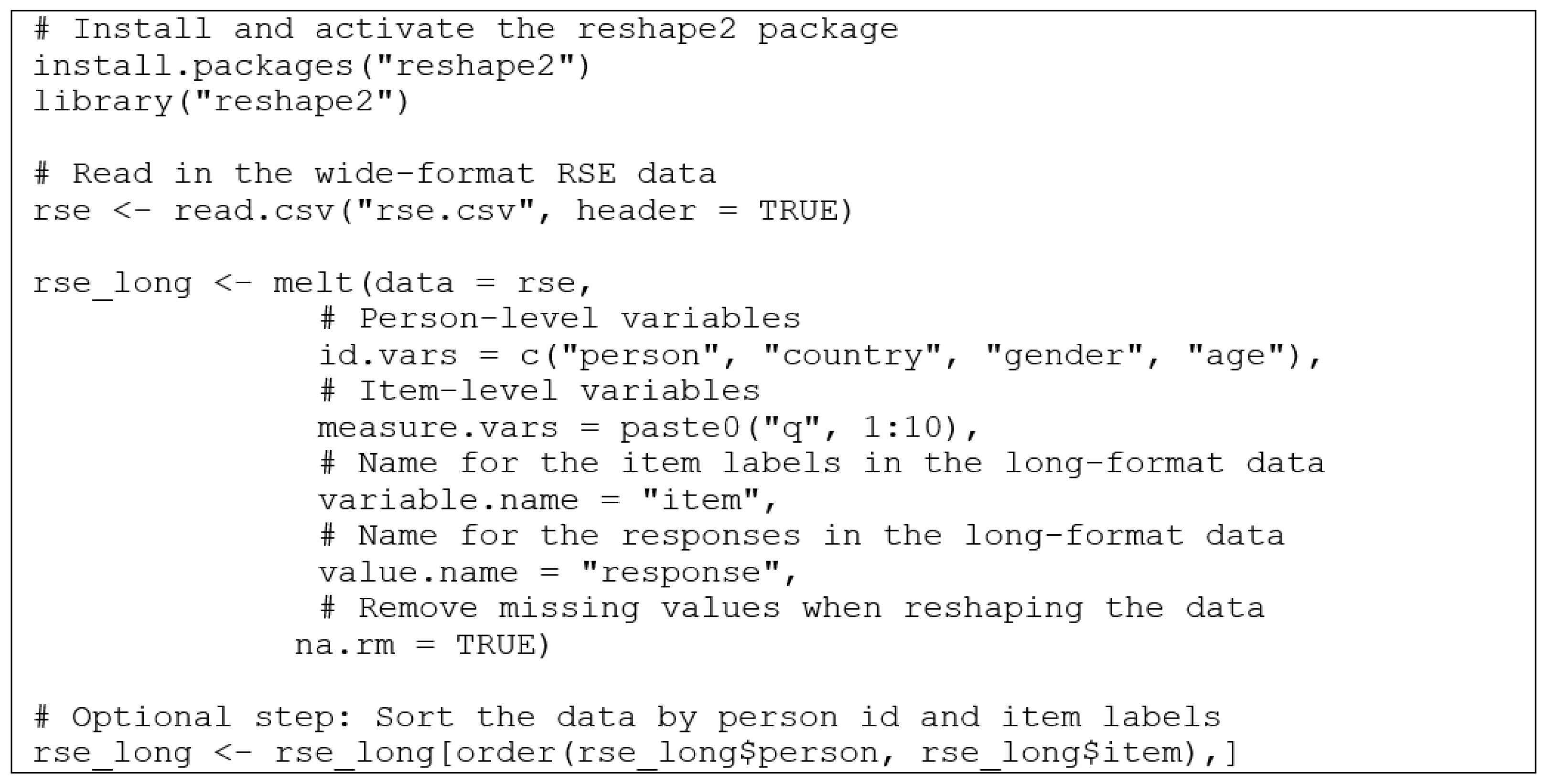
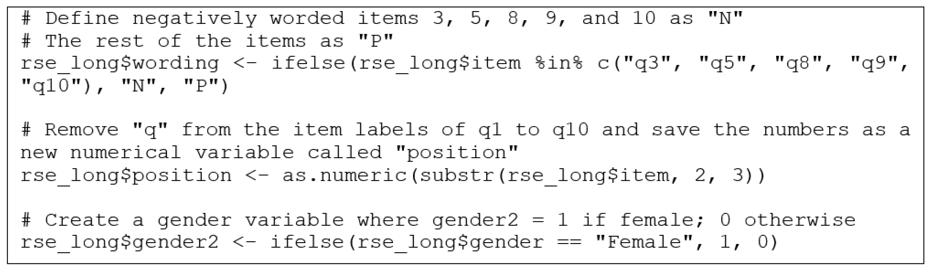
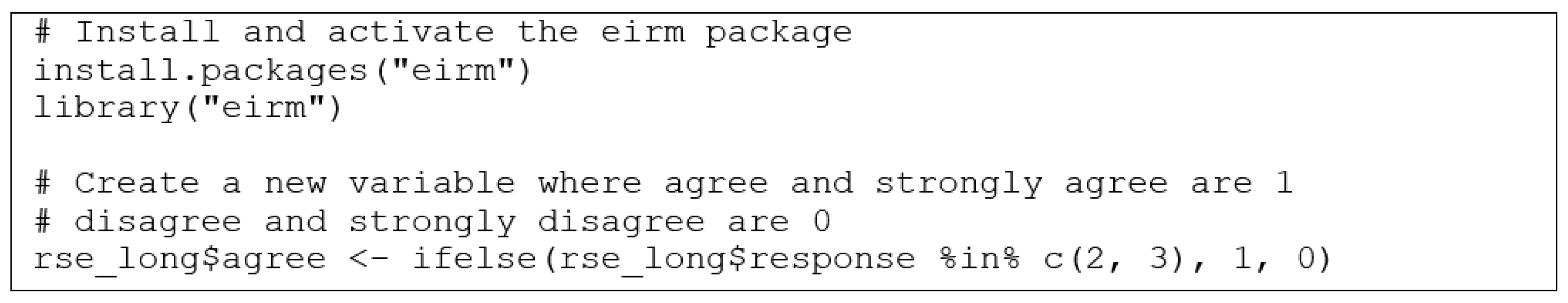
2.1. Data Preparation

As explained earlier, explanatory IRT models following the GLMM framework assume a multilevel structure where item responses (level 1) are repeated observations nested within persons (level 2). It is also possible to estimate explanatory IRT models as cross-classified multilevel models where both items and persons are considered random effects. For more information about such models, see [38]. To accommodate this multilevel structure in the data, the eirm package requires the response data to be in a long format. Response data obtained from educational and psychological instruments are often compiled within a wide-format structure in which a person’s responses will be in a single row and each response is in a separate column. Before using the eirm package, the wide-format data must be restructured as long-format data in which each row represents one item and thus each person has multiple rows. That is, we can see repeated observations (i.e., items) as multiple rows for each person. In long-format data, the person-level variables that do not change across the items remain the same (e.g., gender), while the other variables varying at the item level (e.g., item content) have different values across the rows.
In our example, we use data from the RSE scale (rse.csv) that consists of 961 respondents’ answers to 10 items based on a 4-point Likert scale (ranging from 0 strongly disagree to 3 strongly agree). In the data, responses to negatively-phrased items (i.e., items 3, 5, 8, 9, and 10) are reversed-coded to place all the items in the positive direction (i.e., higher response values are likely to indicate higher self-esteem unless threshold locations are disordered). The data also contain a pseudo identification number and three demographic variables (i.e., country, gender, and age) for each respondent. To prepare the data for subsequent analyses, we use the melt() function in the reshape2 package [39] and transform the data from a wide format to a long format (see Figure 1).
A snapshot of the difference between the wide-format and long-format versions of the RSE data can be seen in Table 1. Unlike in the wide-format data, items in the long-format data are nested within persons and thus the same person has multiple rows (i.e., the same person has 10 rows representing 10 items in the RSE dataset).
In the second step, we use the long-format data to define item-level predictors (i.e., item properties) based on whether the items were negatively worded (denoted with N) or positively worded (denoted with P) and the position of the items in the RSE scale (i.e., 1 to 10). Finally, we create a binary numerical version of the gender variable that will be used as a person-level predictor (i.e., a person property) in the explanatory IRT models (see Figure 2).

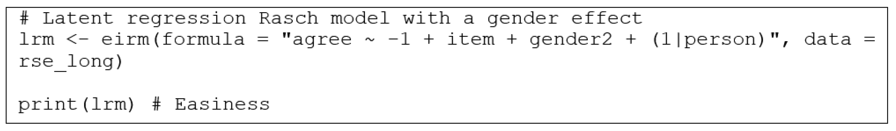
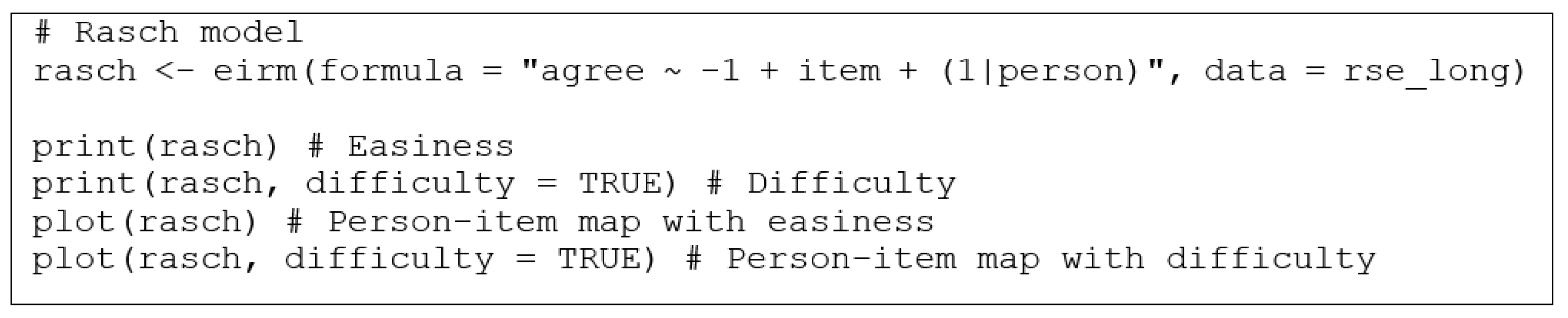
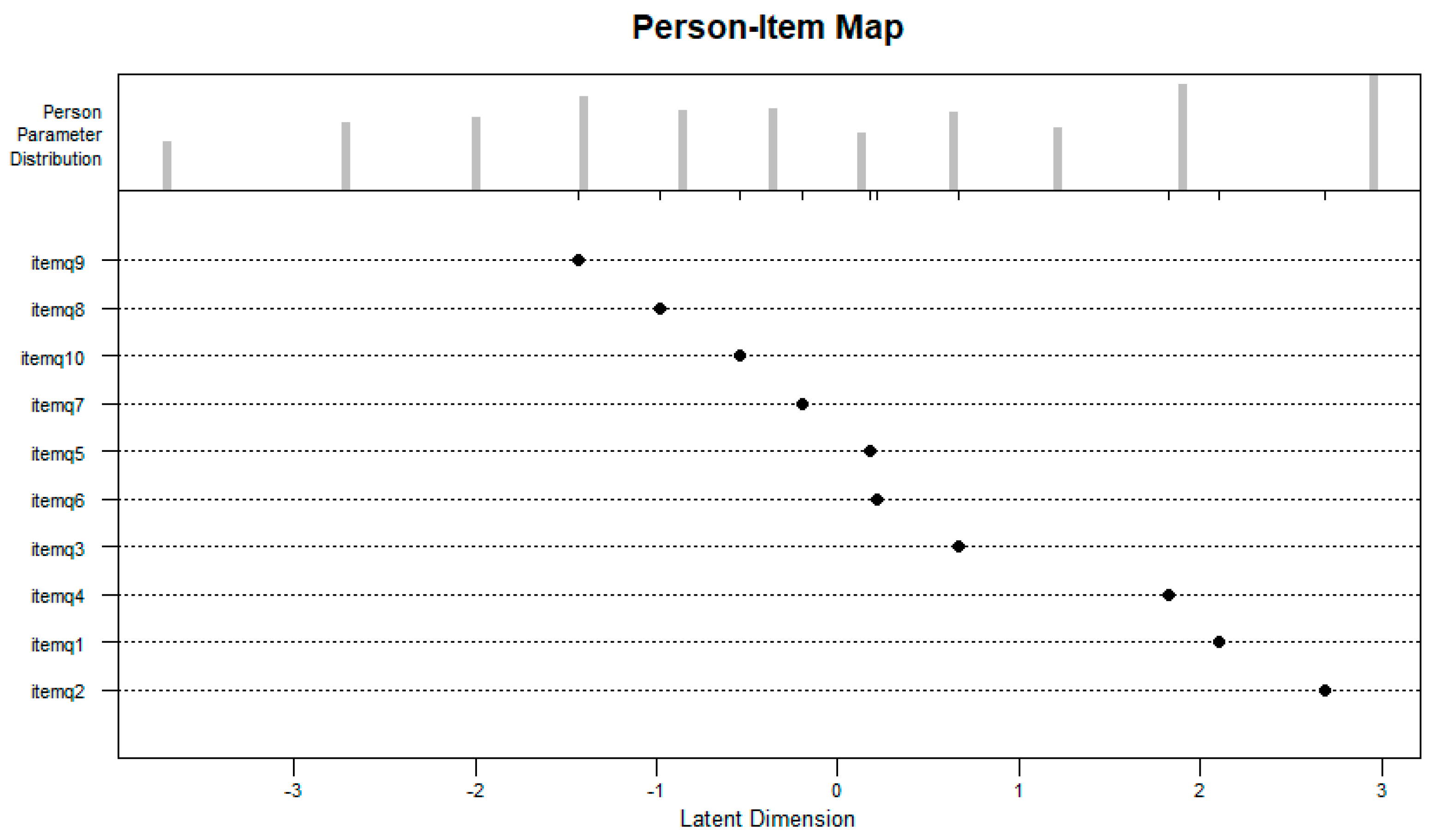
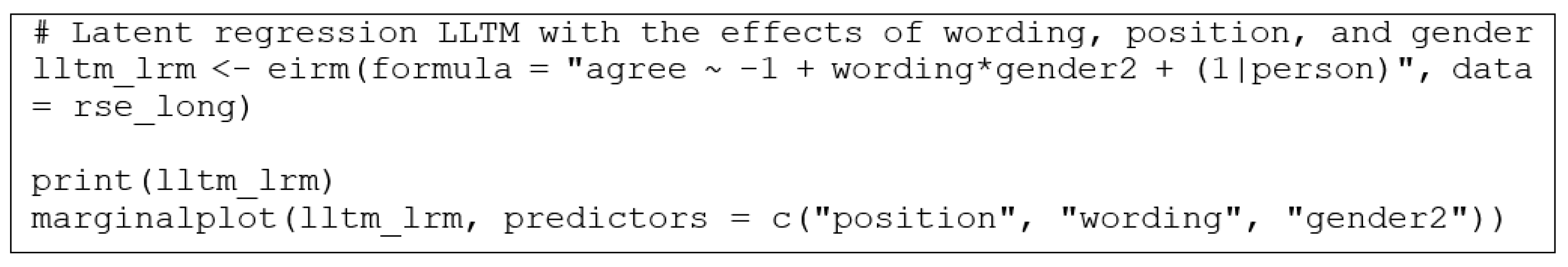
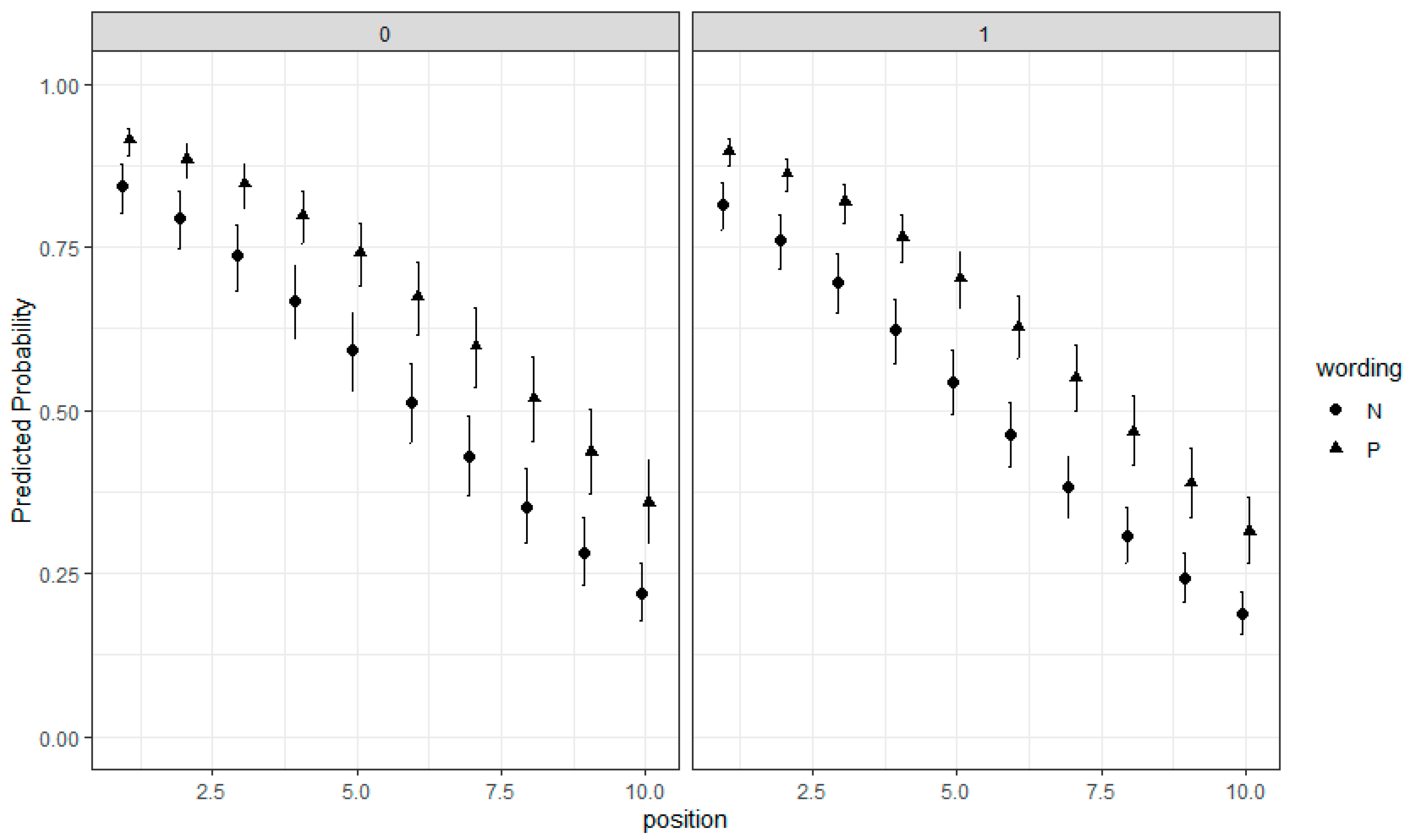
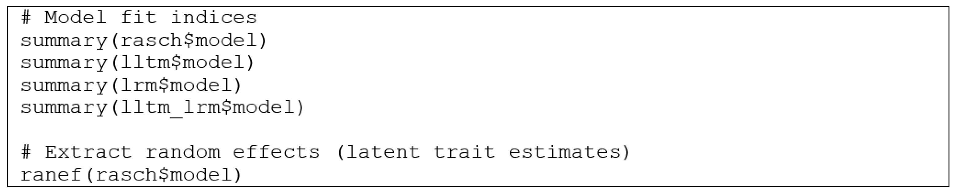
2.2. EIRM for Dichotomous Responses

The following examples show how to use item and person properties to explain dichotomous responses in the long-format RSE dataset. First, we install and activate the eirm package. The eirm package version 0.4 is currently available on the Comprehensive R Archive Network (CRAN; https://cran.r-project.org/ (accessed on 28 July 2021) and can be downloaded using the install.packages() function in R. We also create a new response variable called “agree” by recoding the response categories of strongly agree and agree as 1 and strongly disagree and disagree as 0 to obtain a binary variable of agreement (see Figure 3). We will use the new response variable to demonstrate explanatory IRT models available for dichotomous responses. We will begin with the Rasch model (i.e., a fully descriptive model) as the baseline model and then continue with LLTM (i.e., item explanatory), latent regression Rasch (i.e., person explanatory), and latent regression LLTM (i.e., doubly explanatory).
To estimate the Rasch model for the RSE dataset, we will use the eirm() function, which is the primary function to estimate explanatory IRT models in the eirm package. The eirm() function requires a regression-like formula where a dependent variable (i.e., agree) and predictors (i.e., item) should be defined:
formula = “agree ~ -1 + item + (1|person)”,
where “agree” is the variable for dichotomous responses, “-1” removes the intercept from the model and gives parameter estimates for all items (otherwise, the parameter for the first item becomes the intercept, and the parameters for the remaining items are estimated as the difference from the intercept), “item” represents the item labels (or identifiers) in the dataset, and “(1|person)” refers to the random effects for persons represented by the “person” variable in the dataset. By default, the eirm() function estimates an easiness parameter for each item using a logit link function because it uses a regression model parameterization where positive parameters indicate positive association with the dependent variable.
After model estimation is completed, users can set “difficulty=TRUE” in the print() function to view the difficulty parameters (i.e., easiness * -1). It should be noted that the estimated model parameters for both items and respondents are only point estimates (i.e., a posterior distribution is not available for the estimated parameters). The plot() function can be used to visualize the estimated item parameters (either difficulty or easiness), along with the estimated latent trait levels, in a person–item map (i.e., Wright map). Figure 4 shows the R codes to estimate the Rasch model and print the model output.
Figure 5 shows the person–item map for the Rasch model based on the estimated easiness parameters.
Note that Figure 5 is essentially a modified version of the person–item map that the plotPImap() function in the eirm package [40] produces for the Rasch model. The x-axis shows the latent trait continuum, the y-axis shows the item labels, the locations of the points (on the x-axis) indicate the easiness parameters for the items, and the bars at the top of the plot show the distribution of the latent trait estimates. Users can modify figure aesthetics such as labels of the x and y axes and the figure title.
To estimate explanatory IRT models (e.g., LLTM, latent regression Rasch model, and latent regression LLTM), a similar regression-like formula should be defined for each model. The LLTM formula to estimate the effects of item wording and item position is as follows:
formula = “agree ~ -1 + wording + position + (1|person)”,
where “wording” and “position” are the item properties that are expected to influence how the respondents answered the items on the RSE scale. If LLTM yields statistically significant effects for these item properties, it would indicate the importance of item wording and item position as explanatory variables for the RSE scale (see Figure 6).
The regression-like formula of the latent regression Rasch model to estimate the gender effect (i.e., person property) is defined as follows:
formula = “agree ~ -1 + item + gender2 + (1|person)”,
where “gender2” is a categorical person property (i.e., a person-level predictor). Note that the formula includes “item” to estimate the item difficulty (or easiness) parameters for the items. Thus, there is no item property involved in the model. This model yields individual parameters for the items, latent trait estimates for the respondents, and an overall gender effect. Including gender as a predictor may improve the estimation of person parameters but will not necessarily impact the estimates of item parameters (see Figure 7).
Finally, we demonstrate the latent regression LLTM model that includes both item and person properties as predictors of agreeing with the items on the RSE scale (i.e., the “agree” variable is the dependent variable). This is a doubly explanatory model because the item properties (item wording and item position) explain the item-level variation and gender explains the person-level variation in the RSE dataset. The following formula shows how to define the latent regression LLTM model for the eirm() function:
formula = “agree ~ -1 + wording + position + gender2 + (1|person)”.
In addition to printing the model output, the marginalplot() function can be used to visualize the marginal effects in the latent regression LLTM model. This function uses the ggeffects package [41] to calculate the marginal effects and the ggplot2 package [42] to create a plot. The marginal effect plot will show the predicted probability of agreeing with the RSE items because of the interaction among item position, wording, and gender (see Figure 8).
Figure 9 shows the marginal effect plot for the latent regression LLTM model. There are two separate plots for female (1) and male (0) respondents. The x-axis represents item positions (ranging from 1 to 10) and the y-axis represents the predicted probability of agreeing with the RSE items (ranging from 0 to 1). The plot shows how the predicted probability changes depending on item positions and item wording for each gender group. For both gender groups, the predicted probability decreases as item position increases. In addition, the positively worded items seem to have a higher predicted probability for both female and male respondents, compared with the negatively worded items. The latent regression LLTM model can be further extended by adding an interaction term between item and person properties (e.g., wording*gender2). For more information on the interpretation of the estimated effects for item and person properties, as well as their interactions, readers can review De Boeck et al. [30], Bulut et al. [19], and Stanke and Bulut [16].
Although the eirm() function returns the model output as an eirm object, it still retains the original model output from the lme4 package (i.e., a glmerMod object). Therefore, the helper functions designed for the lme4 package can be used to extract additional information from the estimated models (see Figure 10). For example, relative model fit indices, such as the Akaike information criterion (AIC), the Bayesian information criterion (BIC), and deviance statistics, can be extracted from the models using the summary() function in R, and the ranef() function can be used to extract the random effects (i.e., latent trait estimates).

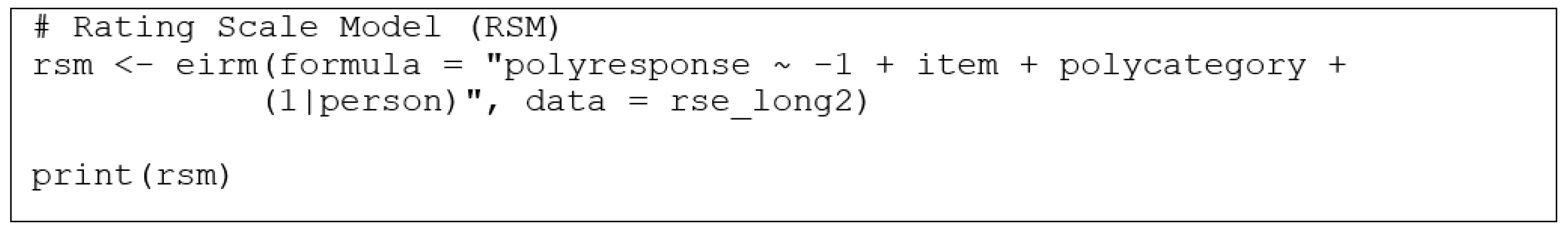
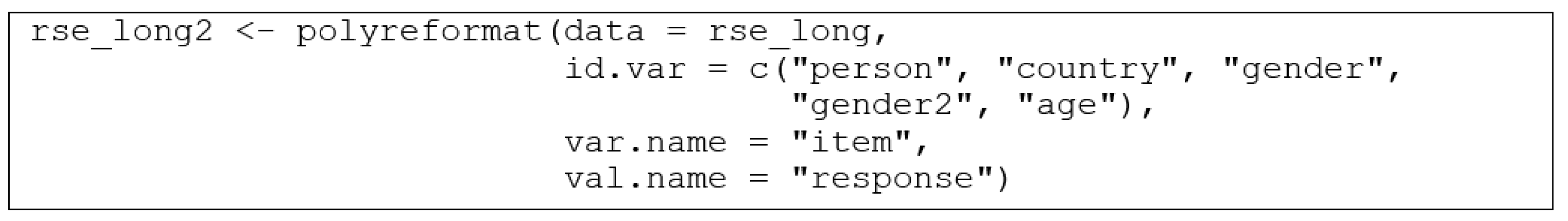
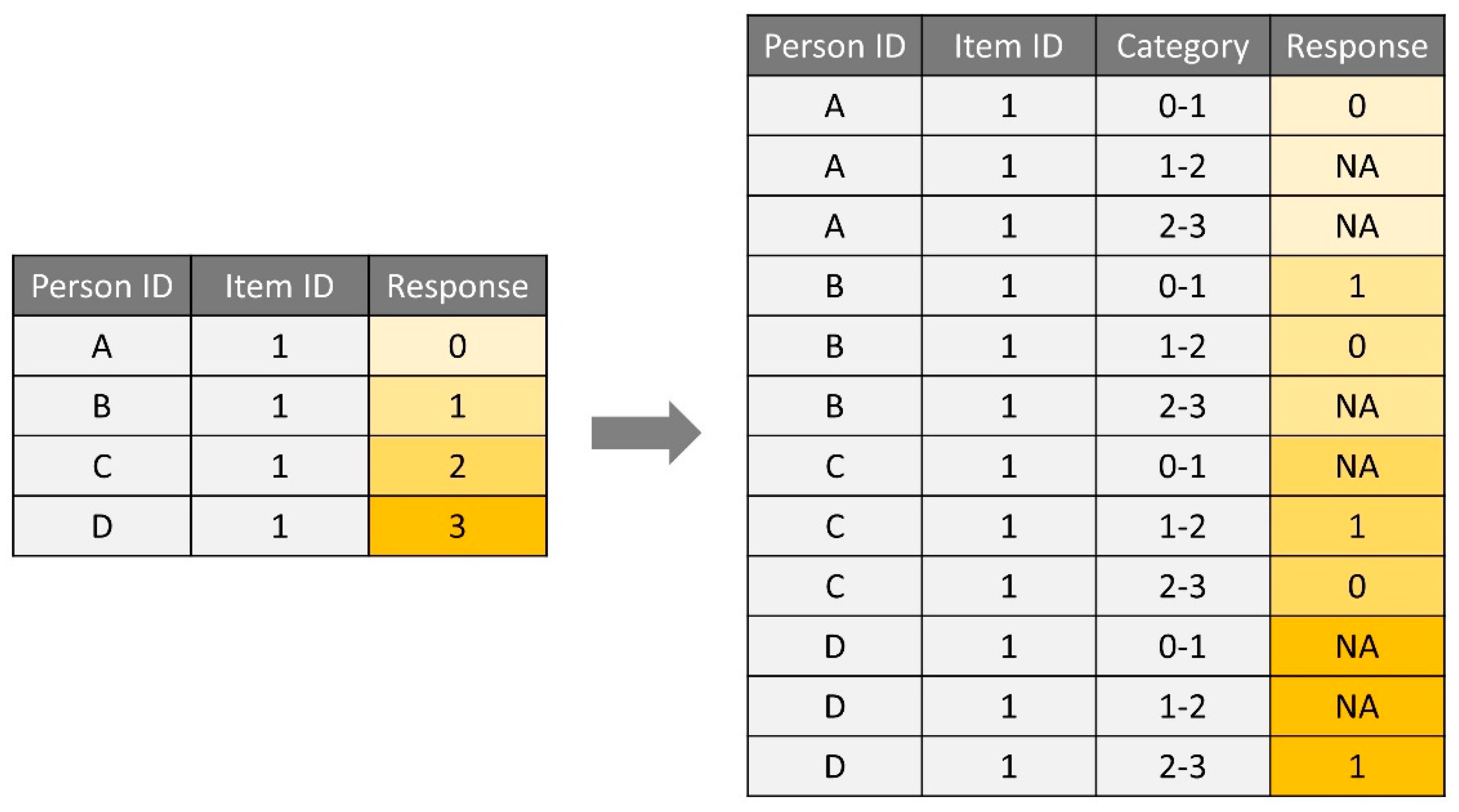
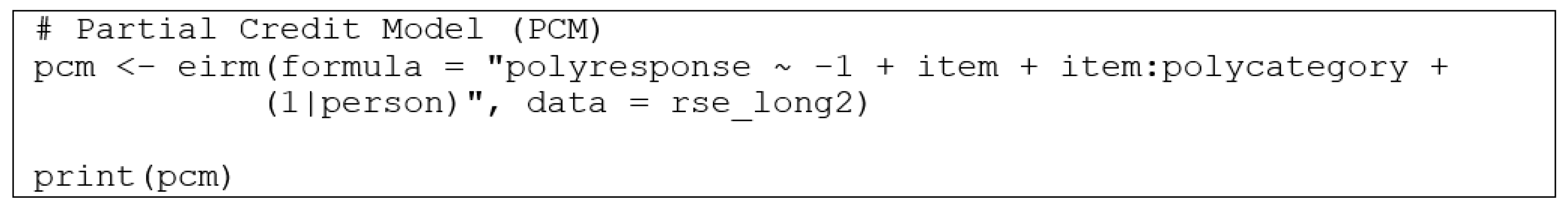
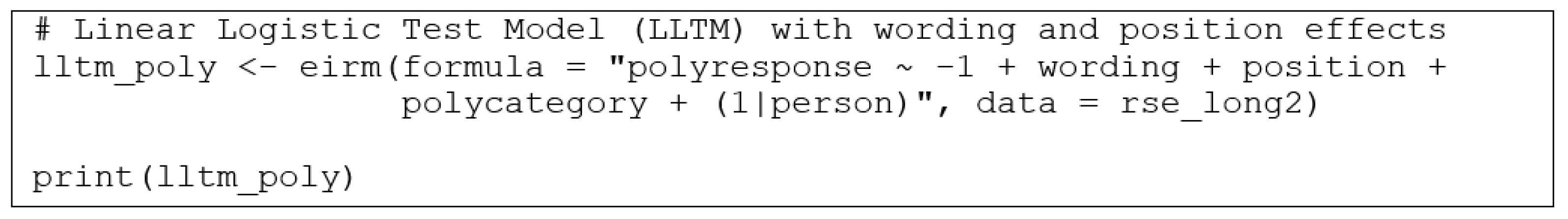
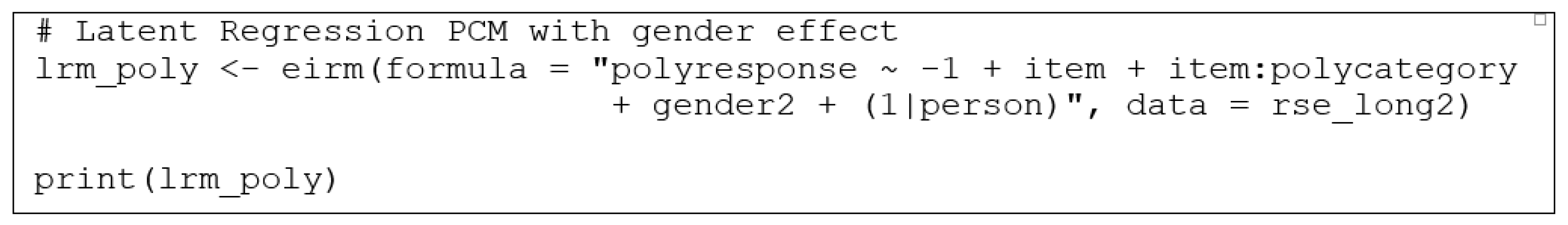
2.3. EIRM for Polytomous Responses

As an extension of the lme4 package, the eirm package also assumes that item responses follow a binomial distribution. One implication of using a binomial distribution is that the dependent variable (i.e., item responses) must be dichotomous. Therefore, polytomously-scored items with ordered response categories (e.g., Likert-scale items) cannot be used as a dependent variable. To tackle this problem, the polyreformat() function in the eirm package allows users to reorganize polytomous responses by creating a set of pseudo-dichotomous responses from the original (ordinal) responses. The polyreformat() function elongates the long-format data by adding new rows depending on the number of response categories in the polytomous items (see [16] for more details on the polyreformat procedure). It must be noted that the polyreformat() function assumes ordered response categories (i.e., ordinal scale), and thus polytomous responses with nominal response categories should not be restructured using this function. In the following example, we use the RSE items with response categories of 0 (strongly disagree) to 3 (strongly agree) to illustrate how the polyreformat() function reorganizes polytomous responses (see Figure 11).
In this example, we use long-format data (rse_long) when reformatting polytomous responses. The polyreformat() function can also reshape wide-format data into long format data if the original dataset is not already in the long format. After defining the person-level variables (i.e., id.var), the variable name that indicates the item labels (var.name), and the variable names that indicate the response values (val.name), the polyreformat() function creates a series of dummy-coded responses based on the polytomous responses and adds two new columns to the data: “polyresponse” and “polycategory”. The “polyresponse” column represents the dummy-coded responses (0, 1, or NA) and the “polycategory” column represents which response category combinations have been used when creating the dummy-coded responses. In the reformatted RSE dataset (rse_long2), each item has three rows, representing the adjacent response category combinations of 0-1, 1-2, and 2-3. Therefore, there are three values for the “polycategory” column: Cat_1, Cat_2, and Cat_3. Figure 12 demonstrates how each polytomous response category is dichotomized in the new dataset. For example, if a respondent selected the response category of 0, then the dummy-coded responses for this polytomous response would be 0 for 0-1 (Cat_1) and NA for 1-2 (Cat_2) and 2-3 (Cat_3). This indicates that the respondent selected the former (0) of the first two adjacent response categories (0 and 1). Since the selected response category is neither 2 nor 3, Cat_2 and Cat_3 remain missing (i.e., NA).
Using the reformatted dataset (rse_long2), it is possible to estimate a variety of descriptive and explanatory IRT models. For example, a Rating Scale Model (RSM; [43]) can be estimated using “polyresponse” as the dependent variable and both “item” and “polycategory” as the predictors:
formula = "polyresponse ~ −1 + item + polycategory + (1|person)".
This model yields a unique location parameter for each item (based on “item”) and a set of threshold parameters that are fixed across all the items in the RSE scale (based on “polycategory”). Figure 13 shows the R codes to estimate the RSM.
In addition to RSM, PCM can be estimated similarly. Unlike RSM with fixed threshold parameters across the items, PCM estimates unique threshold parameters for each item. To estimate PCM, the formula needs to be modified by adding an interaction between “item” and “polycategory”:
formula = "polyresponse ~ −1 + item + item:polycategory + (1|person)",
where “item:polycategory” indicates that we want to estimate unique threshold parameters through an interaction between the items and the response categories. In the formula above, “item” estimates the first threshold parameter (Cat_1), and “item:polycategory” estimates the other threshold parameters (Cat_2 and Cat_3) as distances from the first threshold parameter (see Figure 14).
Once the polytomous response dataset is reorganized using the polyreformat() function, the explanatory IRT models available for dichotomous responses (i.e., LLTM, latent regression model, and latent regression LLTM) can also be estimated with polytomous responses. For example, LLTM can be used to explain the effects of item properties on the threshold parameters, while the latent regression model can be used to explain the effect of person properties on the latent trait levels. In the following example, we use “wording” and “position” as item properties to estimate their impact on the threshold parameters. By default, the item properties explain the first threshold parameter in the items. To explain the other threshold parameters, the model can be expanded with interaction terms between the item properties and “polycategory” (see Figure 15).
formula = “polyresponse ~ −1 + wording + position + polycategory + (1|person)”.
Our final example demonstrates a latent regression PCM with gender (gender2) as a person property (see Figure 16). The model estimates unique threshold parameters for the items (based on “item” and “item:polycategory”) and a gender effect (based on “gender2”). The formula for this model is as follows:
formula = “polyresponse ~ −1 + item + item:polycategory + gender2 + (1|person)”.

3. Discussion

After De Boeck and Wilson [2] introduced the idea of extending traditional IRT models by incorporating item and person properties as predictors, many researchers and practitioners began to implement EIRM to examine how item and person properties can explain common variability stemming from the shared variance among item clusters and person groups. Unlike a fully descriptive IRT model (e.g., Rasch model, PCM, RSM), an explanatory IRT model can involve external predictors (either categorical or continuous) to further describe items in terms of difficulty or persons regarding latent trait levels. Therefore, EIRM allows researchers and practitioners to utilize the IRT framework for both measurement and explanation purposes [2]. A wide range of EIRM applications in the literature include analysis of group differences [3,44,45], differential item and facet functioning (e.g., [17,18]), item position effects (e.g., [12,46]), and item parameter drift (e.g., [19,47]).
In 2011, De Boeck et al.’s [30] detailed tutorial in the Journal of Statistical Software described how to estimate explanatory IRT models with the lme4 package in R. Since then, several researchers have created additional R packages that extended the capabilities of lme4 (e.g., [34,35]). In this tutorial paper, we demonstrate the eirm package, which offers simple tools for estimating explanatory IRT models, extracting model output, and visualizing model outcomes in R. Using real data from the RSE scale and annotated R codes, we aim to promote the eirm package to make it more accessible to a broad range of audiences. Researchers and practitioners can utilize the eirm package to estimate traditional IRT models (e.g., Rasch, PCM, and RSM), item-explanatory models (i.e., LLTM), person-explanatory models (i.e., latent regression models), and doubly explanatory models (i.e., latent regression LLTM) for both dichotomous and polytomous responses. In addition, the polyreformat() function in the eirm package helps users transform polytomous responses into a series of dummy-coded responses to meet the binominal distribution requirement in lme4.

Limitations

There are several limitations when using the eirm package to estimate explanatory IRT models. First, the eirm package is only capable of estimating explanatory IRT models based on the Rasch family of models. Therefore, explanatory IRT models that involve discrimination parameters (e.g., LLTM with discrimination parameters, Generalized Partial Credit Model, and Graded Response Model) cannot be estimated using the eirm package. The mirt package [48] and R packages focusing on latent variable modeling could be viable alternatives when estimating more complex versions of the explanatory IRT models presented in this tutorial. A second limitation of the eirm package is that despite employing a different optimizer to speed up the estimation process, computation time may increase substantially depending on the number of items and persons in the response data and the number of parameters to be estimated in the model (i.e., model complexity). Third, the eirm package only yields points estimates for model parameters. Users who are interested in obtaining posterior distributions of model parameters in a Bayesian setting can use other R packages, such as blme [49] and brms [50]. Finally, the eirm package does not include any functions to simulate response data based on explanatory IRT models. For users who are interested in Monte Carlo simulations with explanatory IRT models, other R packages such as TAM [51] and eRm [38] may be better alternatives.

Author Contributions

Conceptualization, O.B.; methodology, O.B.; software, O.B.; formal analysis, O.B., G.G. and S.N.Y.-E.; investigation, O.B., G.G. and S.N.Y.-E.; writing—original draft preparation, O.B., G.G. and S.N.Y.-E.; writing—review and editing, O.B. All authors have read and agreed to the published version of the manuscript.

Funding

This research received no external funding.

Institutional Review Board Statement

Not applicable.

Informed Consent Statement

Not applicable.

Data Availability Statement

Data used in this study can be downloaded from the following link: https://osf.io/eapd8/ (accessed on 28 July 2021).

Conflicts of Interest

The authors declare no conflict of interest.

References

  1. Wilson, M.; De Boeck, P.; Carstensen, C.H. Explanatory item response models: A brief introduction. In Assessment of Competencies in Educational Contexts; Hartig, J., Klieme, E., Leutner, D., Eds.; Hogrefe & Huber Publishers: Göttingen, Germany, 2008; pp. 91–120. [Google Scholar]
  2. De Boeck, P.; Wilson, M. Explanatory Item Response Models: A Generalized Linear and Nonlinear Approach; Springer: New York, NY, USA, 2004. [Google Scholar]
  3. Briggs, D.C. Using explanatory item response models to analyze group differences in science achievement. Appl. Meas. Educ. 2008, 21, 89–118. [Google Scholar] [CrossRef]
  4. American Educational Research Association; American Psychological Association; National Council on Measurement in Education. Standards for Educational and Psychological Testing; American Educational Research Association: Washington, DC, USA, 2014. [Google Scholar]
  5. Fahrmeir, L.; Tutz, G. Models for multicategorical responses: Multivariate extensions of generalized linear models. In Multivariate Statistical Modelling Based on Generalized Linear Models; Springer: New York, NY, USA, 2001; pp. 69–137. [Google Scholar]
  6. McCulloch, C.E.; Searle, S.R. Generalized, Linear, and Mixed Models; Wiley: New York, NY, USA, 2001. [Google Scholar]
  7. Rasch, G. Studies in Mathematical Psychology: 1. Probabilistic Models for Some Intelligence and Attainment Tests; Nielsen and Lydiche: Oxford, UK, 1960. [Google Scholar]
  8. Rasch, G. Probabilistic Models for Some Intelligence and Attainment Tests; University of Chicago Press: Chicago, IL, USA, 1980. [Google Scholar]
  9. Masters, G.N. A Rasch model for partial credit scoring. Psychometrika 1982, 47, 149–174. [Google Scholar] [CrossRef]
  10. Andrich, D. A rating formulation for ordered response categories. Psychometrika 1978, 43, 561–573. [Google Scholar] [CrossRef]
  11. Fischer, G.H. The linear logistic test model as an instrument in educational research. Acta Psychol. 1973, 37, 359–374. [Google Scholar] [CrossRef]
  12. Hohensinn, C.; Kubinger, K.D.; Reif, M.; Holocher-Ertl, S.; Khorramdel, L.; Frebort, M. Examining item-position effects in large-scale assessment using the Linear Logistic Test Model. Psychol. Sci. Q. 2008, 50, 391–402. [Google Scholar]
  13. Hohensinn, C.; Kubinger, K.D. Applying item response theory methods to examine the impact of different response formats. Educ. Psychol. Meas. 2011, 71, 732–746. [Google Scholar] [CrossRef]
  14. Adams, R.J.; Wilson, M.; Wu, M. Multilevel item response models: An approach to errors in variables regression. J. Educ. Behav. Stat. 1997, 22, 47–76. [Google Scholar] [CrossRef]
  15. Kim, J.; Wilson, M. Polytomous item explanatory item response theory models. Educ. Psychol. Meas. 2020, 80, 726–755. [Google Scholar] [CrossRef]
  16. Stanke, L.; Bulut, O. Explanatory item response models for polytomous item responses. Int. J. Assess. Tool Educ. 2019, 6, 259–278. [Google Scholar] [CrossRef]
  17. French, B.F.; Finch, W.H. Hierarchical logistic regression: Accounting for multilevel data in DIF detection. J. Educ. Meas. 2010, 47, 299–317. [Google Scholar] [CrossRef]
  18. Kan, A.; Bulut, O. Examining the relationship between gender DIF and language complexity in mathematics assessments. Int. J. Test. 2014, 14, 245–264. [Google Scholar] [CrossRef]
  19. Bulut, O.; Palma, J.; Rodriguez, M.C.; Stanke, L. Evaluating measurement invariance in the measurement of development assets in Latino English language groups across development stages. Sage Open 2015, 5, 1–18. [Google Scholar] [CrossRef] [Green Version]
  20. Cho, S.J.; Athay, M.; Preacher, K.J. Measuring change for a multidimensional test using a generalized explanatory longitudinal item response model. Brit. J. Math Stat. Psy. 2013, 66, 353–381. [Google Scholar] [CrossRef]
  21. Qian, M.; Wang, X. Illustration of multilevel explanatory IRT model DIF testing with the creative thinking scale. J. Creat. Think. 2020, 54, 1021–1027. [Google Scholar] [CrossRef]
  22. Sulis, I.; Tolan, M.D. Introduction to multilevel item response theory analysis: Descriptive and explanatory models. J. Early Adolesc. 2017, 37, 85–128. [Google Scholar] [CrossRef]
  23. De Boeck, P.; Partchev, I. IRTrees: Tree-based item response models of the GLMM family. J. Stat. Softw. 2012, 48, 1–28. [Google Scholar] [CrossRef] [Green Version]
  24. Plieninger, H. Developing and applying IR-tree models: Guidelines, caveats, and an extension to multiple groups. Organ. Res. Methods 2021, 24, 654–670. [Google Scholar] [CrossRef] [Green Version]
  25. Rabe-Hesketh, S.; Skrondal, A.; Pickles, A. GLLAMM Manual, UC Berkeley Division of Biostatistics Working Paper Series, Paper No. 160; University of California, Berkeley: Berkeley, CA, USA, 2004; Available online: http://biostat.jhsph.edu/~fdominic/teaching/bio656/software/gllamm.manual.pdf (accessed on 12 July 2021).
  26. Tan, T.K.; Serena, L.W.S.; Hogan, D. Rasch Model and Beyond with PROC GLIMMIX: A Better Choice. Center for Research in Pedagogy and Practice, Paper No. 348-2011; Center for Research in Pedagogy and Practice, Nanyang Technological University: Singapore, 2011; Available online: http://support.sas.com/resources/papers/proceedings11/348-2011.pdf (accessed on 12 July 2021).
  27. Hoffman, L. Example 6: Explanatory IRT Models as Crossed Random Effects Models in SAS GLIMMIX and STATA MELOGIT Using Laplace Maximum Likelihood Estimation. Available online: https://www.lesahoffman.com/PSQF7375_Clustered/PSQF7375_Clustered_Example6_Explanatory_Crossed_MLM.pdf (accessed on 12 July 2021).
  28. Wu, M.L.; Adams, R.J.; Wilson, M.R. ConQuest: Multi-aspect Test Software [Computer Program]; Australian Council for Educational Research: Melbourne, Australia, 1997. [Google Scholar]
  29. Muthen, L.K.; Muthen, B.O. Mplus User’s Guide; Muthen & Muthen: Los Angeles, CA, USA, 1998–2019. [Google Scholar]
  30. De Boeck, P.; Bakker, M.; Zwitser, R.; Nivard, M.; Hofman, A.; Tuerlinckx, F.; Partchev, I. The estimation of item response models with the lmer function from the lme4 package in R. J. Stat. Softw. 2011, 39, 1–28. [Google Scholar] [CrossRef] [Green Version]
  31. Bates, D.; Mächler, M.; Bolker, B.; Walker, S. Fitting linear mixed-effects models using lme4. arXiv 2014, arXiv:1406.5823. [Google Scholar]
  32. R Core Team. R: A Language and Environment for Statistical Computing; R Foundation for Statistical Computing: Vienna, Austria, 2021. [Google Scholar]
  33. Petscher, Y.; Compton, D.L.; Steacy, L.; Kinnon, H. Past perspectives and new opportunities for the explanatory item response model. Ann. Dyslexia. 2020, 70, 160–179. [Google Scholar] [CrossRef]
  34. Bulut, O. eirm: Explanatory Item Response Modeling for Dichotomous and Polytomous Item Responses. R Package Version 0.4. 2021. Available online: https://CRAN.R-project.org/package=eirm (accessed on 12 July 2021).
  35. Jeon, M.; Rockwood, N. PLmixed. R Package Version 0.1.5. 2020. Available online: https://cran.r-project.org/web/packages/PLmixed/index.html (accessed on 12 July 2021).
  36. Rosenberg, M. Rosenberg self-esteem scale (RSE). Accept. Commit. Ther. Meas. Package 1965, 61, 18. [Google Scholar]
  37. Rosenberg, M. Society and Adolescent Self-Image; Princeton University Press: Princeton, NJ, USA, 1965. [Google Scholar]
  38. De Boeck, P. Random item IRT models. Psychometrika 2008, 73, 533–559. [Google Scholar] [CrossRef]
  39. Wickham, H. Reshaping data with the reshape package. J. Stat. Softw. 2007, 21, 1–20. [Google Scholar] [CrossRef]
  40. Mair, P.; Hatzinger, R. Extended Rasch modeling: The eRm package for the application of IRT models in R. J. Stat. Softw. 2007, 20, 1–20. [Google Scholar] [CrossRef] [Green Version]
  41. Lüdecke, D. ggeffects: Tidy data frames of marginal effects from regression models. J. Open Source Softw. 2018, 3, 772. [Google Scholar] [CrossRef] [Green Version]
  42. Wickham, H. ggplot2: Elegant Graphics for Data Analysis; Springer: New York, NY, USA, 2016. [Google Scholar]
  43. Andrich, D. An extension of the Rasch model for ratings providing both location and dispersion parameters. Psychometrika 1982, 47, 105–113. [Google Scholar] [CrossRef]
  44. Yau, D.T.; Wong, M.C.; Lam, K.F.; McGrath, C. Longitudinal measurement invariance and explanatory IRT models for adolescents’ oral health-related quality of life. Health Qual. Life Out. 2018, 16, 60. [Google Scholar] [CrossRef] [Green Version]
  45. Albano, A.D.; Rodriguez, M.C. Examining differential math performance by gender and opportunity to learn. Educ. Psychol. Meas. 2013, 73, 836–856. [Google Scholar] [CrossRef] [Green Version]
  46. Albano, A.D. Multilevel modeling of item position effects. J. Educ. Meas. 2013, 50, 408–426. [Google Scholar] [CrossRef]
  47. Stanke, L.; Bulut, O.; Rodriguez, M.C.; Palma, J. Investigating Linear and Nonlinear Item Parameter Drift with Explanatory IRT Models. Presented at the National Council on Measurement in Education, Washington, DC, USA, 7–8 April 2016. [Google Scholar]
  48. Chalmers, R.P. mirt: A multidimensional item response theory package for the R environment. J. Stat. Softw. 2012, 48, 1–29. [Google Scholar] [CrossRef] [Green Version]
  49. Dorie, V.; Bates, D.; Maechler, M.; Bolker, B.; Walker, S. Blme: Bayesian Linear Mixed-Effects Models. R Package Version 1.0-5. Available online: https://CRAN.R-project.org/package=blme (accessed on 23 July 2021).
  50. Bürkner, P.-C.; Gabry, J.; Weber, S.; Johnson, A.; Modrak, M. Brms: Bayesian Regression Models Using ‘Stan’. R Package Version 2.15.0. Available online: https://CRAN.R-project.org/package=brms (accessed on 23 July 2021).
  51. Robitzsch, A.; Kiefer, T.; Wu, M. TAM: Test. Analysis Modules. R Package Version 3.7-16. Available online: https://CRAN.R-project.org/package=TAM (accessed on 12 July 2021).
Figure 1. Transform the wide-format RSE data to the long-format data.
Psych 03 00023 g001
Figure 2. Creating item-level and person-level predictors.
Psych 03 00023 g002
Figure 3. Install and activate the eirm package and create a new response variable.
Psych 03 00023 g003
Figure 4. Estimate the Rasch model and print the model output.
Psych 03 00023 g004
Figure 5. This person–item map based on the Rasch model.
Psych 03 00023 g005
Figure 6. Estimate the LLTM model and print the model output.
Psych 03 00023 g006
Figure 7. Estimate the latent regression Rasch model and print the model output.
Psych 03 00023 g007
Figure 8. Estimate the latent regression LLTM and print the model output.
Psych 03 00023 g008
Figure 9. Estimate the latent regression LLTM and print the model output (Note. 1 = Female and 0 = Male. ▲= Positively-worded items and ● = Negatively-worded items. Position refers to the positions of the items on the RSE scale. Error bars indicate the 95% confidence interval around the predicted probability values).
Psych 03 00023 g009
Figure 10. Extract additional information from the explanatory IRT models.
Psych 03 00023 g010
Figure 11. Convert polytomous responses to pseudo-dichotomous responses.
Psych 03 00023 g011
Figure 12. An example of how polytomous responses are defined as pseudo-dichotomous responses.
Psych 03 00023 g012
Figure 13. Estimate the Rating Scale Model and print the model output.
Psych 03 00023 g013
Figure 14. Estimate the partial credit model and print the model output.
Psych 03 00023 g014
Figure 15. Estimate the LLTM for polytomous items and print the model output.
Psych 03 00023 g015
Figure 16. Estimate the latent regression PCM and print the model output.
Psych 03 00023 g016
Table 1. First five rows of wide and long format data.
Wide FormatLong Format
Personq1q2q3PersonItemResponse
12231q12
22201q22
31101q33
42221q43
52221q52
Publisher’s Note: MDPI stays neutral with regard to jurisdictional claims in published maps and institutional affiliations.

