Next Article in Journal / Special Issue
Evaluating Cluster-Level Factor Models with lavaan and Mplus
Previous Article in Journal / Special Issue
Automated Test Assembly in R: The eatATA Package
 
 
Please note that, as of 22 March 2024, Psych has been renamed to Psychology International and is now published here.
Article

How to Estimate Absolute-Error Components in Structural Equation Models of Generalizability Theory

by
Terrence D. Jorgensen
Department of Child Development and Education, University of Amsterdam, Postbus 15776, 1001 NG Amsterdam, The Netherlands
Psych 2021, 3(2), 113-133; https://doi.org/10.3390/psych3020011
Submission received: 10 April 2021 / Revised: 25 May 2021 / Accepted: 26 May 2021 / Published: 29 May 2021

Abstract

:
Structural equation modeling (SEM) has been proposed to estimate generalizability theory (GT) variance components, primarily focusing on estimating relative error to calculate generalizability coefficients. Proposals for estimating absolute-error components have given the impression that a separate SEM must be fitted to a transposed data matrix. This paper uses real and simulated data to demonstrate how a single SEM can be specified to estimate absolute error (and thus dependability) by placing appropriate constraints on the mean structure, as well as thresholds (when used for ordinal measures). Using the R packages lavaan and gtheory, different estimators are compared for normal and discrete measurements. Limitations of SEM for GT are demonstrated using multirater data from a planned missing-data design, and an important remaining area for future development is discussed.

1. Introduction

After discussing coefficient α as a measure of scale reliability [1], Cronbach et al. [2] began developing a more comprehensive framework capable of assessing reliability not only among a set of tests (or scale items) measuring the same latent construct, but also among any other method of obtaining measurements, such as multiple raters, occasions, or tasks. Generalizability theory [GT] [2,3] extends classical test theory [CTT] [4] by differentiating between a (theoretically) unlimited number of independent sources of measurement error, rather than a single conflated error term. Beyond its value for scale development [5], the versatility of GT has been demonstrated by applications in a wide variety of psychological domains, such as clinical/counseling [6,7,8], personality assessment [9,10], and education sciences [11,12,13]. GT can simultaneously quantify reliability of several types that are of common interest in psychological disciplines, including scale reliability, test–retest reliability, and interrater reliability (IRR).
Marcoulides [14] proposed specifying a GT design as a structural equation model [SEM]; see also [15] to estimate GT variance components—an idea recently revisited by Vispoel et al. [16], who also extended the idea to SEM with ordinal variables [17]. Applications of SEM to GT have so far focused only on obtaining a generalizability coefficient (G-coef), which is defined using only relative error. Thus, a G-coef quantifies reliability of decisions based on relative rather than absolute differences in scores. In many research scenarios, a G-coef is sufficient because its interpretation is relevant when using a composite (e.g., taking the mean of all measurements, like a scale mean) as an observed variable in a regression or correlation analysis.
However, researchers might also be interested in quantifying the dependability of their measurements, which is relevant when using a composite score to classify subjects into categories (e.g., making a diagnosis or identifying the need for intervention). In this case, (global or cut-score-specific) D-coefficients are defined using absolute error. If, for example, the facet of generalization is raters (who each provide measurements about a set of N subjects), a G-coef would quantify norm-referenced consistency (i.e., consistency among raters’ rank-ordering of subjects), whereas a D-coef would be criterion referenced (i.e., agreement among raters about each subject’s absolute level of the construct being measured). Absolute error includes the same variance components as relative error, plus additional components that cannot be specified as SEM parameters simultaneously with relative-error variance components.
Transposing the data matrix has been proposed to estimate absolute-error variance components [15]. Transposition puts subjects in rows rather than columns, so correlations between subjects are the basis for inferring common-variance components due to a facet of generalization. Ark [18] (p. 54) described this “Q method” as “laborious” and “cumbersome because they must perform a separate analysis for each facet of generalization”. The method also becomes infeasible in the very common case that there are more rows (subjects) of data than columns (measurement conditions). To correct a possible misconception that the drawbacks of the Q-method would limit a researcher to computing a relative G-coef [18,19], I show how absolute-error variance components can be indirectly captured as functions of parameters in the same SEM that estimates relative-error variance components.
Using the open-source R [20] package lavaan [21], I demonstrate with simulated data how to specify appropriate constraints on the mean structure of a confirmatory factor analysis (CFA) model to represent the remaining facets necessary for absolute error in designs with one and two (crossed and nested) facets. Whereas [14,15,17] calculated point estimates of G- and D-coefs after fitting the model, I demonstrate how to define them as new parameters in lavaan’s model syntax, thus additionally obtaining a delta-method standard error (SE) and normal-theory confidence interval (CI) for G- and D-coefs. Because the delta method relies on asymptotic theory, it can yield poor coverage and inflated Type I errors in small or modest samples. Thus, I also demonstrate how to obtain Monte Carlo CIs, which is a more robust method because it only assumes the estimated parameters (not complex functions of parameters) have normal sampling distributions [22]. For ordinal data—for which G-coefs have been defined on a latent-response metric [17,18]—I show how the same mean-structure constraints can be specified in combination with appropriate constraints on thresholds. I use a real-data example to demonstrate some limiting conditions under which SEM becomes infeasible for estimating GT variance components, in which case a mixed-effects modeling framework would be more promising.

2. Materials and Methods

The only materials necessary to conduct and replicate the analyses in this article are a computer with the R statistical software environment (at least version 4.0), with the lavaan, semTools, and gtheory add-on packages installed and loaded into the workspace. At the time of this writing, I used lavaan version 0.6-8, semTools version 0.5-4, and gtheory version 0.1.2.
No human-subjects data were gathered for this article. For illustrative analyses in this section, I used example data provided with the semTools package, loaded into the R workspace by running data(exLong) after loading the semTools library. Originally simulated for the longInvariance() function’s help-page example, these data include 3 (items) × 3 (occasions) = 9 measurements of N = 200 subjects. Note that G-study designs use factorial notation similar to ANOVA; in fact, analyses of G-study data using mean-squares estimators of variance components have been termed GENOVA [3].
Throughout the examples, I assume that the objects of measurement (the facet of differentiation) are human subjects—the persons facet—which must be represented as rows of input data. Distinct measurements of the facet of differentiation must be represented in different columns of input data. In these example data, the facets of generalization are n i = 3 items and n o = 3 occasions, yielding nine measurements to be used as indicators in a CFA. As pointed out by [16] [p. 6] and by [17] [p. 161], this design facilitates disentangling different types of measurement error—namely, specific-factor error (i.e., how interindividual differences vary across items) and transient error (i.e., how interindividual differences vary across occasions)—from random-response measurement error. A “one-facet design” (i.e., one facet of generalization) is incapable of disentangling different sources of measurement error. To illustrate a one-facet design, I use only the three items on the first occasion in the example below. Further details about notational conventions can be found in [3,16].
The remainder of this section describes the methods to specify CFAs for data from one-facet, two-nested-facet, and two-crossed-facet G-studies (these map onto the first three examples presented by [17] in their online supplementary materials), which include an appropriately constrained mean structure to represent main and interaction effects involving facets of generalization. I then discretize the example data and illustrate (a) how to model the mean structure with ordinal measurements, (b) how to obtain G- and D-coefs on the LRV scale, and (c) how to use existing software to obtain a G-coef on the ordinal response scale (see Section 5.3). All R syntax to replicate analyses in this article can be found on the Open Science Framework (OSF; [23]). Results are presented in the following section.

2.1. One-Facet Design: Persons × Items

In a p × i design, the observed measurements Y p i are a linear combination of a grand mean μ , main effects of both persons ( β p = μ p μ ) and items ( β i = μ i μ ), and the interaction between persons and items ( β p i = μ p i μ p μ i + μ ), the latter of which is conflated with any other sources of measurement error:
Y p i = μ + ( μ p μ ) + ( μ i μ ) + ( μ p i μ p μ i + μ ) = μ + β p + β i + β p i ,
where any μ represents a mean and any β represents an effect (discrepancy from a mean). Given independent effects (each with mean β ¯ = 0 ), the total variance of Y p i is a sum of the variances of the components:
σ Y 2 = σ p 2 + σ i 2 + σ p i 2 .
Again, the highest-order term is also conflated with any other sources of measurement error. The G- and D-coefs are equivalent to intraclass correlation coefficients (ICCs) that express the magnitude of universe-score variance relative to random and systematic sources of error variance [24]. Relative error is used to quantify consistency or generalizability of items:
G - coef p × i = ICC ( C , n i ) = σ p 2 σ p 2 + σ p i 2 n i ,
which is equivalent to coefficient α [1,16] because the only facet of generalization is items and Equation (1) is consistent with essential tau-equivalence. (i.e., all indicators are equally related to their underlying construct, represented in CFA by equating factor loadings across indicators). Note that traditionally, GT additionally assumes that items are randomly parallel, which is represented in CFA by equating not only factor loadings but also residual variances. Vispoel et al. [25] have recently explored how these assumptions can be relaxed in the SEM framework.
Absolute error is used to quantify agreement or dependability of items:
D - coef p × i = ICC ( A , n i ) = σ p 2 σ p 2 + σ i 2 + σ p i 2 n i .
A more specific D-coef for the use of a particular cut-score can be calculated by adding its squared distance from the mean to both the numerator and denominator:
D - coef c u t , p × i = σ p 2 + ( μ c u t ) 2 σ p 2 + ( μ c u t ) 2 + σ i 2 + σ p i 2 n i .
The further a cut-score is from the mean, the more dependable the scale would be when making criterion-based decisions. When c u t = μ , Equation (5) reduces to the global D-coef (Equation (4)) and takes its lowest value, so I only present cut-score equations in later sections. Plots can illustrate how D-coefs vary across a range of cut-scores [16,17].
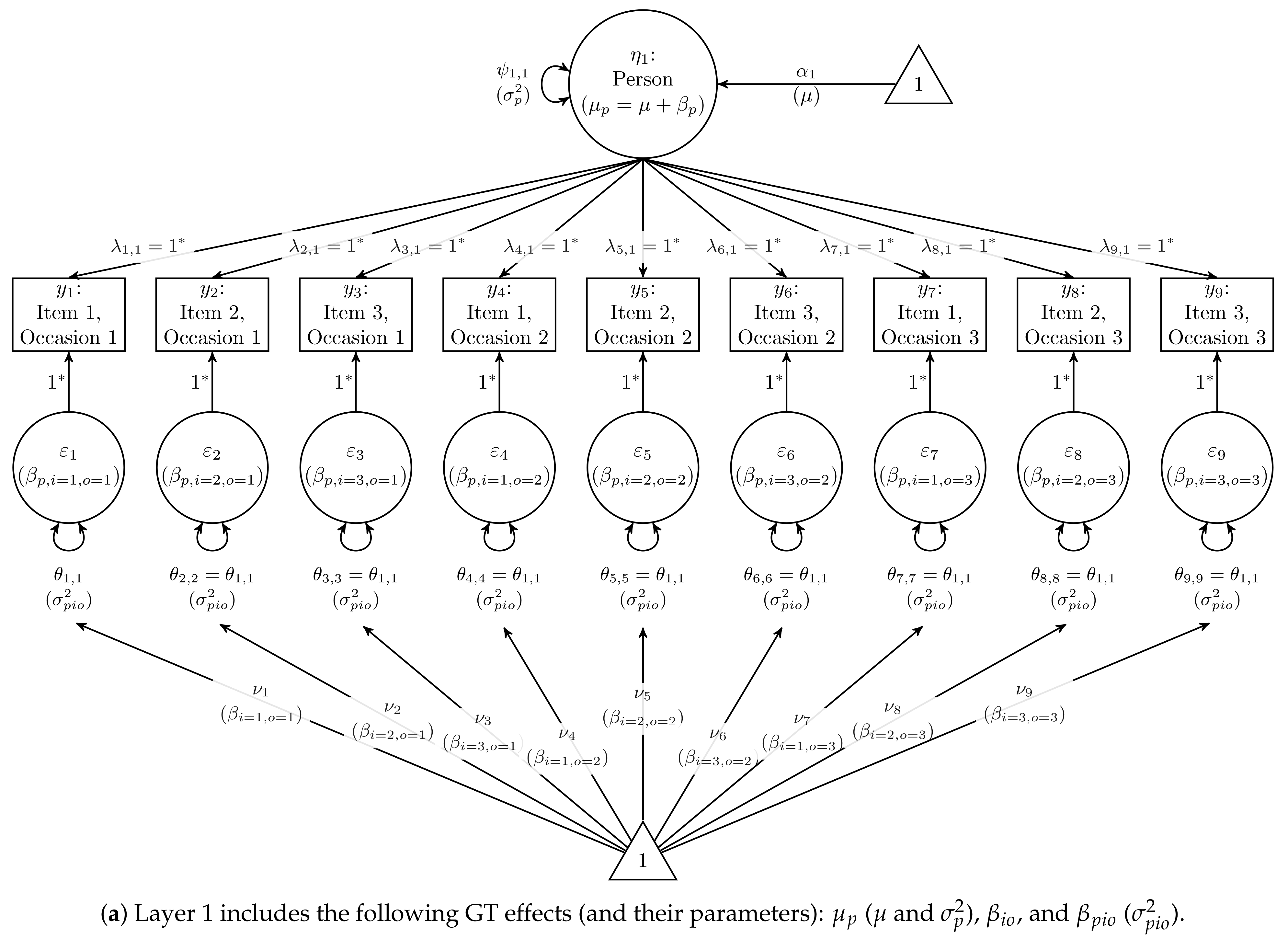
For this example, I used only the measurements on Occasion 1, so the path diagram in Figure 1 omits any reference to occasions. Figure 1 represents a CFA in which each condition of measurement is an indicator of a common factor. Thus, subjects’ factor scores are analogous to their universe scores in the GT framework and are the source of common variance among the measurements. Consistent with the GT assumption that measures are randomly parallel [2,16], all factor loadings are fixed to λ = 1 .
Because variances of common or unique factors in a CFA represent variability across rows of data (the facet of differentiation: persons), only variance components with a p subscript are directly estimable with CFA. The variance of the Person factor ( ψ 1 , 1 in Figure 1) is analogous to σ p 2 and the unique-factor (residual) variances ( θ i , i ) are analogous to σ p i 2 . Whereas [14,17] allowed θ i , i to differ across items and averaged the residual variances after fitting the model to obtain a single estimate of σ p i 2 , the residual variances could instead be constrained to equality across items [15], as reflected by the labels in Figure 1.
The remaining variance component is σ i 2 , which is not a CFA model parameter. Previous authors [15,18] indicated that σ i 2 could only be obtained by fitting a separate CFA model to a transposed data matrix, with an Item common factor and each person as an indicator. However, this leads to estimation problems because typically, N > p (i.e., there would be more columns than rows of data) [17] [p. 158]. Furthermore, estimating σ i 2 in a separate CFA prevents users from defining a D-coef parameter or obtaining its delta-method or Monte Carlo CI. Instead, σ i 2 can be defined as a function of mean-structure parameters, as shown in the top row of Table 1. In Figure 1, the item intercepts can be estimated under the constraint that their average is 0, which enables the factor mean to be freely estimated. This is the effects-coding identification constraint for the mean structure [26], which ensures the mean of the Person factor is interpreted as the grand mean μ . Likewise, an item intercept ( ν i ) is the difference between the item mean ( μ i ) and the grand mean ( μ ), so the intercepts are the item effects. The estimated item variance is thus the sample variance of the estimated vector ν :
σ ^ i 2 = 1 n i 1 i = 1 n i ν ^ i 2 .
Equation (6) can be used to define a new parameter in SEM software syntax such as Mplus [27] or lavaan [21] to obtain a maximum likelihood (ML) estimate of σ i 2 . Likewise, the R script on OSF also shows how to specify the G- and D-coefs (Equations (3) and (4), respectively) as new parameters in lavaan syntax.

2.2. Two-Facet Crossed Design: Persons × Items × Occasions

A p × i × o model for observed measurements Y p i o extends Equation (1) by adding a main effect of occasions ( β o = μ o μ ) and three interaction terms ( β p o , β i o , and β p i o ):
Y p i o = μ + β p + β i + β o + β p i + β p o + β i o + β p i o .
As in any GT design, the highest-order interaction is conflated with any other sources of measurement error, and the marginal variance is a sum of the variance components:
σ Y 2 = σ p 2 + σ i 2 + σ o 2 + σ p i 2 + σ p o 2 + σ i o 2 + σ p i o 2 .
It may also be informative to calculate the proportion of specific-factor ( σ p i 2 ) and transient ( σ p o 2 ) error, relative to total (including random-response: σ p i o 2 ) error; see [17] [p. 161, Equations (14)–(16)]. The G-coef is defined using relative error (terms with p subscripts):
G - coef p × i × o = σ p 2 σ p 2 + σ p i 2 n i + σ p o 2 n o + σ p i o 2 n i × n o ,
which quantifies generalizability across both items and occasions—“a coefficient of equivalence and stability” [17] [p. 161, Equation (17)]. However, G-coefs can also quantify generalizability separately across each dimension, analogous to coefficients for scale reliability and test–retest reliability [17] [p. 161, Equations (18) and (19), respectively]. Again, a D-coef is defined using absolute error, which additionally includes components of effects that do not vary across persons:
D - coef c u t , p × i × o = σ p 2 + ( μ c u t ) 2 σ p 2 + ( μ c u t ) 2 + σ i 2 + σ p i 2 n i + σ o 2 + σ p o 2 n o + σ i o 2 + σ p i o 2 n i × n o .
Equation (10) collapses to a global D-coef when c u t = μ .
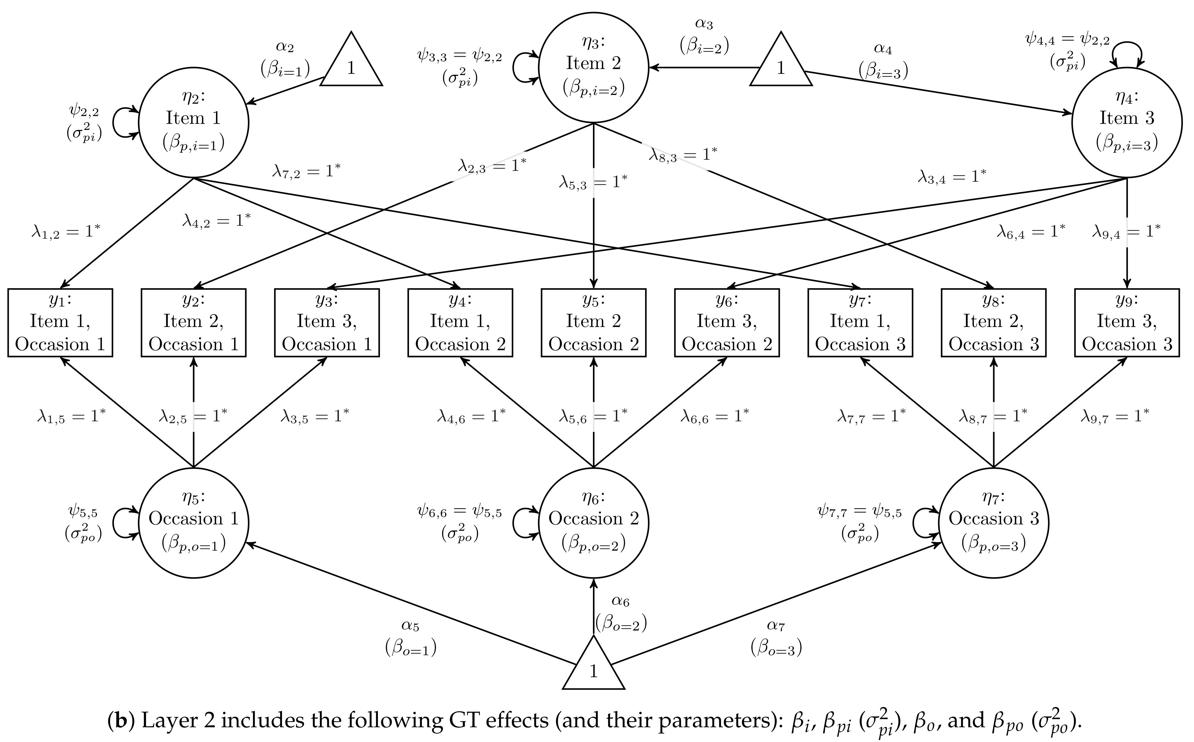
Figure 2 depicts a CFA for all nine measurements of the example data, where each of three items were administered on each of three occasions. The factor-loading matrix consists only of zeros and ones that map indicators onto their respective components (see Figure 2). Again, all measurements are indicators of a common Person factor, but additional minor factors can be added to represent levels of multiple facets of generalization. In this case, all Item-1 measurements are indicators of a common Item 1 factor (likewise for Items 2 and 3), and all Occasion-1 measurements are indicators of a common Occasion 1 factor (likewise for Occasions 2 and 3).
As with unique factors, the variances of the minor factors represent variability across persons within a particular measurement condition, so
  • all Item factor scores represent the β p i effects, and the Item factor variances are constrained to equality to represent σ p i 2 ;
  • all Occasion factor scores represent the β p o effects, and the Occasion factor variances are constrained to equality to represent σ p o 2 ;
  • all unique-factor scores (indicator residuals) represent the β p i o effects, and the residual variances are constrained to equality to represent σ p i o 2 .
The remaining variance components are σ i 2 , σ o 2 , and σ i o 2 . Because these do not include any variance across persons, those effects are constants, which can be reflected in the mean structure. With the appropriate constraints, the Item factor means can represent Item effects ( β i ), the Occasion factor means can represent Occasion effects ( β o ), and the indicator intercepts can represent the Item × Occasion interaction effects ( β i o ).
The two-facet design’s CFA model has seven common factors, so seven constraints must be imposed on the mean structure to identify their means, as listed in Table 1. Recall that each effect ( β * ) is defined as varying around a mean of zero:
  • As with the one-facet model, the factor scores represent μ p = μ + β p , so a freely estimated Person mean represents the grand mean (because β ¯ p = 0 ). To identify this latent mean, impose the effects-coding constraint on all nine indicator intercepts, as shown in the top row of Table 1. This constraint reflects β ¯ i o = 0 , which is equivalent to constraining the sum of β i o = 0 because the mean is merely the sum scaled by 1 / ( n i × n o ) .
  • The effects-coding constraint can also be imposed on the indicators of each item’s factor (e.g., across occasions, Item 1’s indicators sum to zero, shown in Row 2 of Table 1). However, only n i 1 such constraints are needed because the n i th constraint would be redundant given the constraint on all nine intercepts. That is, if n i 1 mutually exclusive subsets each sum to zero, then the remaining subset must also sum to zero in order for the entire set to sum to zero. The final n i th Item factor’s mean is identified by constraining all Item-factor means to sum to zero, consistent with β ¯ i = 0 . The means of Item factors can thus be interpreted as Item effects ( β i ).
  • The same pattern holds for Occasion factors as for Item factors. The effects-coding constraint is placed on the subset of indicators (e.g., across items, Occasion 1’s indicators sum to zero) for n o 1 Occasion factors, and the n o th Occasion factor’s mean is identified by constraining all Occasion means to sum to zero: β ¯ o = 0 . The means of Occasion factors are thus interpreted as Occasion effects ( β o ).
With the appropriate specifications for main and interaction effects among facets of generalization, their variances can be calculated as functions of the estimated common-factor means ( α f ) and measured-variable intercepts ( ν m ).
σ ^ i 2 = 1 n i 1 f = 2 4 α ^ f 2 ,
σ ^ o 2 = 1 n o 1 f = 5 7 α ^ f 2 ,
σ ^ i o 2 = 1 ( n i × n o ) 1 m = 1 n i × n o ν ^ m 2 .
The R script on OSF specifies these functions as new parameters in lavaan syntax to obtain ML estimates of these variance components and the G- and D-coefs defined in Equations (9) and (10), respectively, along with delta-method SEs and Monte Carlo CIs.

2.3. Two-Facet Nested Design: Persons × (Items within Occasions)

A p × ( i : o ) model for observed measurements Y p ( i : o ) resembles Equation (7):
Y p ( i : o ) = μ + β p + β o + β p o + β i : o + β p ( i : o ) ,
but with fewer terms. Person and occasion effects are still fully crossed, but administering a unique set of items on each occasion prevents disaggregating independent item and occasion effects. The main effect of items and the i × o interaction are confounded in the term β i : o . Items are still repeatedly administered across persons, but because item effects cannot be disentangled from the occasion effects in which they are nested, specific-factor error (the p × i interaction) and random-response measurement error (the p × i × o interaction) are confounded in the term β p ( i : o ) .
Using the associated variance decomposition,
σ Y 2 = σ p 2 + σ o 2 + σ p o 2 + σ i : o 2 + σ p ( i : o ) 2 ,
the G-coef is still defined using relative error (all terms with a p subscript):
G - coef p ( i : o ) = σ p 2 σ p 2 + σ p o 2 n o + σ p ( i : o ) 2 n i : o × n o ,
where n i : o is the number of items within each occasion (constant across occasions). Again, the D-coef is defined using absolute error, which additionally includes components of effects that do not vary across persons, and a cut-score-specific D-coef also incorporates a criterion’s distance from μ :
D - coef c u t , p ( i : o ) = σ p 2 + ( μ c u t ) 2 σ p 2 + ( μ c u t ) 2 + σ o 2 + σ p o 2 n o + σ i : o 2 + σ p ( i : o ) 2 n i : o × n o .
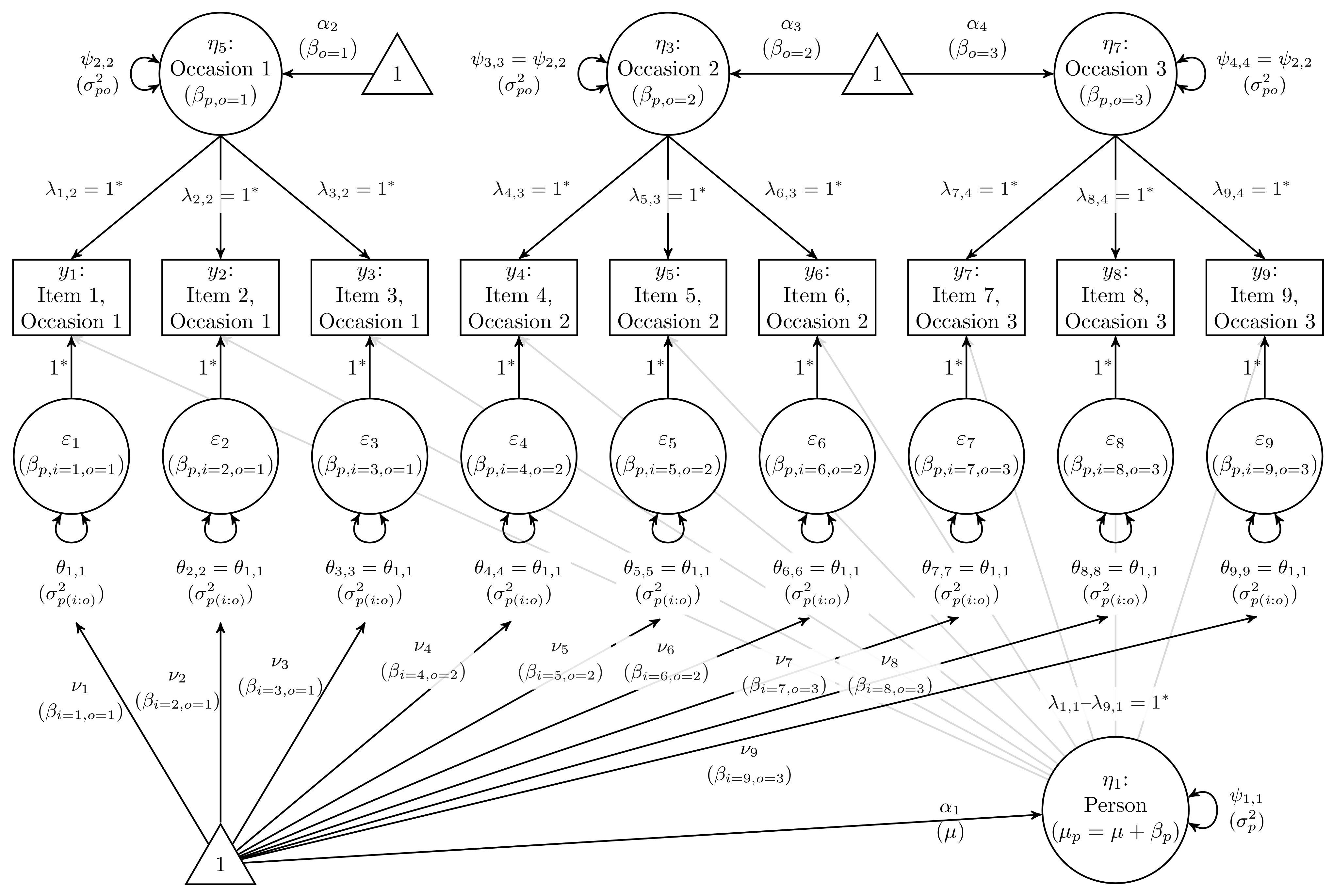
The path diagram in Figure 3 portrays a CFA representing a p × ( i : o ) design.
In the example lavaan syntax on OSF, the nine measurements are treated as though they were nine distinct items—Items 1–3 only on Occasion 1, Items 4–6 only on Occasion 2, and Items 7–9 only on Occasion 3—rather than the same three items on each occasion. Note that it is also possible to derive coefficients for this design from the fully-crossed p × i × o data [17] [pp. 161 & 168–169]. Figure 3 resembles Figure 2 for a fully crossed design, but because each item is measured on only one occasion, no common factors are specified to represent items. The same constraints in Table 1 are used to identify the person and occasion factor means (with the same interpretation as in the p × i × o model), but no constraints are required for the (absent) item factors. The occasion variance is estimated as in Equation () (except the sum is over factors 2–4 rather than 5–7), and Equation (6) can be used to estimate σ i : o 2 rather than σ i 2 .

2.4. Discretized Data

The CFA models described so far were developed in the context of indicators having continuous (e.g., interval-level) scales of measurement, but social science data are often discrete (e.g., binary checklists or ordinal Likert scales). Historically, GT variance components have been estimated by treating ordinal data the same way continuous data would be treated [28], using numeric weights for ordinal categories (e.g., 1–5 for a 5-point Likert scale, or 0–1 for a checklist of binary items). In that case, the methods already described can simply be applied to ordinal measurements as though they were continuous. However, G-coefs have also been estimated for ordinal measurements by capitalizing on the latent response variable (LRV) interpretation commonly used in SEM [17,18]. Item factor analysis [IFA] [29] augments CFA with a threshold model that assumes that an observed discrete variable x represents a crude measurement of a continuous LRV y. Estimators typically assume y (or its residuals) to be normally distributed, which is equivalent to specifying a (cumulative) probit link between a discrete outcome and its linear predictor in the generalized linear model [30] [pp. 122–124]. The same LRV interpretation is available when using a (cumulative) logit link [31] [pp. 187–189], but the LRV’s residuals are assumed to follow a standard logistic distribution (with variance π 2 3 ) rather than a standard normal distribution. This approach has also been explored in item-response theory (IRT) models for GT [32,33,34], some of which are statistically equivalent to IFA models (e.g., the 2-parameter normal-ogive or logit model and analogous graded response models).

2.4.1. The Threshold Model and Latent Response Scales

Using thresholds τ 1 = 0.5 and τ 2 = 1.0 , the example data were discretized into three ordinal categories ( c = 0 , 1, or 2) using the following threshold model:
x p i o = c if τ c < y p i o τ c + 1 ,
with C + 2 thresholds forming boundaries around C + 1 contiguous regions of the y p i o distribution, corresponding to C + 1 categories. Because the normal distribution is unbounded, τ 0 = and τ C + 1 = + by definition, and only the remaining C thresholds are estimable.
Because the y variables in IFA are latent (circles instead of squares in the path diagrams above), the locations and scales of their distributions are arbitrarily chosen, often by fixing their intercepts to ν = 0 and either their marginal or residual variances to 1 [35] (i.e., the delta or theta parameterization, respectively) [36]. This allows all thresholds to be estimated, but an indicator’s intercept can be estimated if a constraint is placed on its threshold(s) [37]. (Constraining a second threshold would allow its marginal or residual variance to be estimated, but that provides no benefit in this context.) Either parameterization is arbitrary, just as common-factor locations and scales are arbitrary [38], but calculations are simpler using the theta parameterization because all residual variances are simply fixed to 1 (i.e., no pooled calculation is required). The constraints listed in the bottom two rows of Table 1 are minimally sufficient to identify the intercepts (i.e., statistically equivalent to estimating all thresholds and fixing all intercepts to zero), so that the mean-structure constraints already described can continue to be used in an IFA for GT.
For the first (or any arbitrarily chosen) measurement, rather than freely estimating all C thresholds, they can be estimated under the constraint that their average is zero. This allows the LRV intercept to be estimated, analogous to the effects-coding constraint used on intercepts to identify common-factor means [26]. For a binary variable with C = 1 threshold, the constraint is achieved simply by fixing the threshold τ = 0 , in which case the estimated intercept would be equal in magnitude (but with opposite sign) as the estimated threshold when fixing ν = 0 . Thus, a statistically equivalent approach for binary variables would be to simply place the intercept constraints in Table 1 on the thresholds instead, yielding identical estimates of variance components derived from the mean structure. However, this would also change the sign of the estimated Person mean. The final example demonstrates this approach with real multirater binary measurements.
With this constraint in place for one measurement, the thresholds for each remaining measurement can be constrained to equality with the first (or fix all τ = 0 for binary measurements), thus identifying intercepts for the remaining measurements. The estimated intercepts can then be constrained as described in Table 1 such that LRV and factor intercepts represent GT components. Thus, once the threshold model is appropriately constrained, the remaining IFA parameters can be specified using the same principles discussed for CFA parameters above.

2.4.2. Coefficients on Ordinal vs. Latent-Response Scales

The LRV interpretation has also been utilized in CTT by applying the formula for coefficient α to an estimated polychoric correlation matrix instead of a covariance matrix on the observed response scale [39,40]. The LRV interpretation has advantages relative to simply treating ordinal measurements as continuous. Using a threshold model to link observed ordinal responses to LRVs can eliminate scaling irregularities due to transformation and categorization errors [17], which facilitates comparing results across studies that use different scaling metrics (e.g., 3-point vs. 5-point Likert scales). When disattenuating scale-composite correlations for measurement error, G-coefs on the ordinal and LRV scales are quite similar when Likert scales have many points [17]. However, because scale coarseness can be considered one type of measurement error [41]—because the variable being measured is truly continuous—the LRV scale becomes better equipped to fully disattenuate correlations in scales with fewer categories [17,18].
Whereas G- and D-coefs on the LRV scale quantify reliability of ideal or hypothetical data [42], G- and D-coefs on the observed scale quantify the reliability of the data on hand. Thus, treating the ordinal response scale as continuous can also be advantageous, especially when calculating a D-coef for a specific cut-score. Typically, a cut-score is an absolute criterion with reference to the actual scale used for measurements, or some function of it (e.g., the possible range of a scale total). Vispoel et al. [17] [p. 163, Equation (25)] proposed a D-coef on the LRV scale that only required relative-error variance components, based on the assumption that the LRVs were z scores (i.e., μ ^ Y = 0 and σ ^ Y = 1 ). A global D-coef was then equivalent to a G-coef, and cut-scores could be expressed in units of S D but were divorced from the observed response scale.
Vispoel et al. [17] [p. 163] noted their proposed LRV-scale D-coef was limited because “differences among the absolute levels of scores are not taken into account or presumed not to differ.” Another limitation is that their assumption of standardized LRVs is only consistent with the delta parameterization [36], in which the marginal LRV variances are fixed to 1 for identification and residual variances are merely functions of marginal variances and other model parameters (factor loadings and variances) [35]. In order for residual variances to be constrained to equality [15,17] (rather than averaging residual variances across measurements), they must be treated as model parameters by utilizing the theta parameterization [36], in which case they are fixed to 1. In this case, a D-coef equation on the LRV scale [17] [Equation (25] would have to be adapted to allow for marginal LRV variances in excess of 1. Another potential problem with the approach in [17] is that LRV scales were not linked across measurements by constraining thresholds to equality [37].
The threshold-model constraints I proposed above resolve many of these issues. Constraining thresholds to be invariant across measurements allows the latent scales to be linked on a common metric [37]. Constraining each indicator’s thresholds to be distributed around 0 (or fixing a single threshold to 0 for binary indicators) identifies the LRV intercepts, which in turn can be constrained just as they are when indicators are (treated as) continuous (Table 1). Thus, estimates of absolute-error components are available, so standard formulas for global and cut-score-specific D-coefs (Equations (4), (5), (10), and (17)) can be applied without requiring LRVs to be z scores. However, the limitation remains that the chosen cut-score is on the LRV metric rather than the observed discrete response scale, so the cut-score would have to be chosen using a potentially arbitrary heuristic [17] [e.g., 2 S D s away from the mean; p. 166, Equation (32)].

3. Results

All CFA models specified above were fitted to the normally distributed example data from semTools, using MLE in lavaan. For comparison, G- and D-coefs were also calculated using mean-squares (MS, i.e., GENOVA) and restricted ML (REML) estimates, the latter of which are available from the gtheory package [43], which employs the lme4 package [44,45]. The same estimators were also used to calculate G- and D-coefs for the discretized example data, which can be expected to be lower due to reduced variability of the discrete data relative to the untransformed continuous data [46,47] (i.e., categorization error). Finally, IFA models were fitted to the discretized example data, using diagonally weighted least-squares (DWLS) estimation and relying on the LRV interpretation. Because the example data were not simulated to reflect a substantively meaningful response scale (either on the normal or discretized scales), and because LRVs have arbitrary scales, a cut-score of 2 S D s above the mean was used to calculate cut-score-specific D-coefs in all models. Vispoel et al. [17] [p. 166, Equation (32)] made a similar comparison using two S D s below the mean (resulting in the same D-coef as for two S D s above the mean).
Results are presented in Table 2. The R syntax on OSF also demonstrates how to obtain normal-theory CIs via the delta-method in lavaan, as well as Monte Carlo CIs in semTools, the latter of which involves simulating a joint sampling distribution of the parameter estimates (like a parametric bootstrap procedure) and tend to be more robust in smaller samples [22]. I do not present CI results here because they are not the focus of the article, but I do recommend reporting them in practice to help quantify uncertainty. It is noteworthy that the mixed-modeling framework yields identical (to the 5th decimal place) estimates using either (ordinary/unweighted) least-squares or REML estimation. Likewise, the SEM framework yields identical estimates using least-squares (not presented in Table 2) or ML estimation. However, the modeling frameworks do differ in the second or third decimal place because the discrepancy functions differ. The sum-of-squares or negative log-likelihood is minimized with respect to each row of data (i.e., observed vs. predicted casewise scores) in mixed-models but with respect to summary statistics (i.e., observed vs. predicted means and covariance matrix) in SEM.
The top three rows of Table 2 show nearly identical G- and D-coefs across estimators in all three designs. Rows 4–6 show the same trend for the discretized data, but as expected, those coefficients were lower than for truly continuous indicators because continuous indicators capture more information about individual differences. Estimated cut-score-specific D-coefs were more similar between normal and discretized data because of the large distance of the cut-score from the mean. Global D-coefs are generally lower than G-coefs because absolute error includes more variance components than relative error. However, when using a specific cut-score to make absolute decisions, especially one that is far from the mean (here, 2 S D s), the scale is notably more dependable [3,16], as reflected by D-coefs for cut-scores exceeding the G-coefs.
Given that the simulated example data were drawn from a multivariate normal distribution, it is reasonable to use their estimated coefficients as a point of reference to compare estimates on the LRV scale in the penultimate row of Table 2. The generalizability and dependability of ideal or hypothetical latent scores could be informative about the quality of variables that would have been measured on a more approximately continuous scale [42], but less so about the variables actually observed in practice. However, because the illustrative example in fact discretized (simulated) normally distributed data, one should expect the generalizability and dependability on the LRV scale to approximate the G- and D-coefs for the normal data. Table 2 shows that in these discretized data, the estimated IFA parameters (fitted to polychoric correlations among the discretized measurements) yield slightly (roughly 0.01–0.04) higher coefficients than the CFA parameters (fitted to the truly normal observed data that were not discretized). Across models, the DWLS estimates of σ p 2 were proportionally higher than would be expected from fixing the residual variances to θ i , i = 1 . The bottom row of Table 2 is explained in the Discussion.

4. A Multirater Study with Planned Missing Data

A final example with real data illustrates that SEM might be infeasible using certain measurement designs. Whereas there is little additional cost associated with some facets of generalization (e.g., designing additional items or tasks), other facets might carry similar costs to recruiting subjects, such as scheduling additional measurement occasions or recruiting additional raters. Planned missing data (PMD) designs have been proposed as a way to reduce such costs by randomly assigning subjects to complete subsets of items [49,50], to be measured on certain occasions, or both [51]. Although not explicitly referred to as a PMD design, random assignment of raters has also occurred in practice, yielding extremely sparse data from studies that minimized the burden on raters [52,53,54,55].

4.1. Design

In this real-data example [55], observations were made by six physician faculty (r) about 29 first-year internal medicine residents’ (p) communication skills, measured using the Advanced Care Planning Communication Assessment Tool (ACP-CAT) in two task conditions (t). The ACP-CAT is a binary checklist of 20 items (i) and also includes two summative items measured with a Likert scale. Although the study is a three-facet design ( p × r × t × i ), the facets of generalization would yield 6 × 2 × 20 = 240 variables, which makes SEM infeasible given only 29 subjects. I therefore focus primarily on the scale total (ranging 0–20) under one-facet ( p × r ) and two-facet ( p × r × t ) designs, as well as one summative item to discuss potential challenges with ordinal data.
Whereas subjects (persons) and raters were each fully crossed with tasks, not all subject–rater combinations yielded data because Yuen et al. [55] assigned two out of the six participating raters to observe each of the 29 subjects. Nonetheless, subjects and raters were not nested facets because no subset of raters only observed one subject ( r : p ), nor was any subset of subjects observed by only one rater ( p : r ). Subjects and raters could be described as partially crossed because no subject was paired with every rater (or vice versa), but every subject was rated by multiple raters (and every rater observed multiple subjects). With ( 6 × 5 ) / 2 = 15 pairs of raters, each pair of raters was randomly assigned to observe only two of the same subjects in each task, except for one pair of raters (in each task) who only jointly observed a single subject.
Because random assignment ensures a missing completely at random (MCAR) mechanism, pairwise deletion should yield unbiased estimates of each element in the covariance matrix among observed variables [56]. However, the coverage rates (i.e., proportion of observations that can provide information about an estimate) for the covariance matrix was quite low: 34.5% for diagonal cells (variance across subjects for each task–rater combination) and 6.9% for covariances between raters within the same condition. Because random assignment of raters to subjects differed across tasks, the covariance between tasks within each rater had 0% coverage and so could not be calculated (i.e., there was no summary statistic for the SEM to attempt to reproduce). Coverage for other off-diagonal elements ranged from 6.9 to 17.2%. The R syntax on OSF prints a data matrix and summaries that illustrate the missing-data patterns in this design.

4.2. CFAs for the Scale Total

A path diagram for this p × r × t design would resemble Figure 2, but (a) two tasks would replace three items and (b) six raters would replace three occasions. As the example syntax on OSF shows, a properly specified SEM for this GT design does not converge on a ML solution when fit to the example data (also provided on OSF) using full-information ML (FIML) to accommodate incomplete data [19]. Rather than a problem with estimating model parameters, the lavaan package warned that the “maximum number of iterations reached when computing the sample moments using EM” (i.e., not all sample covariances could be estimated), although the error did not indicate that 0% coverage absolutely prevented estimating the model parameters.
A one-factor model was specified for a p × r design—resembling Figure 1 but with six raters instead of three items—and fitted to the data within each task, in which there were no summary statistics with 0% coverage. However, there remained an additional complication: correlations could only take values of 1 , 0, or 1. Correlations could even be undefined when for a pair of raters, one (or both) rater’s scores did not vary among the two subjects jointly observed with the other rater. This necessarily occurred for the pair of raters who only jointly observed one subject within a task, but also when either rater in a pair provided the same scores for both jointly observed subjects (because the variance would be 0 for those two observations). This may be related to the error message when attempting to fit the one-factor model to the Task-2 p × r data: “system is computationally singular”, accompanied by multiple warning messages about trouble estimating the summary statistics, which implies potential linear dependencies therein.
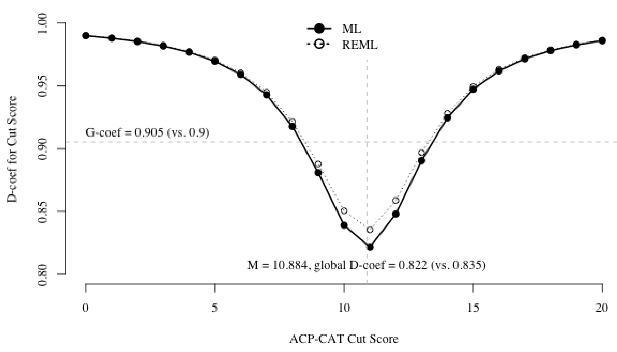
Nonetheless, lavaan was able to find a ML solution for the Task-1 p × r data. The estimated G-coef = 0.905, with Monte Carlo 95% CI [0.833, 0.951], indicated that ACP-CAT scale totals were quite generalizable across raters within Task 1. This G-coef is an IRR coefficient equivalent to ICC(C,2) [24]. Note, however, that in the single-facet p × r design, rater error cannot be disaggregated from error associated with specific tasks—what Vispoel et al. [16] [p. 6] referred to as a “hidden facet” because p × t interaction variance is implicitly absorbed into the numerator’s subject variance, artificially inflating estimated G- and D-coefs. The estimated global D-coef (0.821, 95% CI [0.675, 0.890])—equivalent to ICC(A,2) for IRR [24]—also indicated high dependability when using a cut-score at the mean ( 10.884 11 ) to make decisions about absolute standing of subjects on the ACP-CAT scale. Dependability exceeded 0.90 when using cut-scores <9 or >13; Figure 4 illustrates how dependability varies across the scale’s 0–20 range. As in Table 2, the ML estimates from lavaan were quite similar to the REML estimates from gtheory (G-coef = 0.900, global D-coef = 0.835, also shown in Figure 4), whose mixed-model approach does not have the same estimation challenges of wide-format data.

4.3. IFAs for Discrete Scale Items

IFA models yielded additional challenges associated with estimation of thresholds. In order for estimated thresholds to have the same interpretation across facets of generalization (i.e., columns of wide-format data), the same thresholds—and therefore the same categories—must be observed across facets of generalization. To illustrate this, I use a single binary item provided in the data on OSF. (The eighth ACP-CAT item reads “Encouraged discussing goals/wishes with HCP/family” and is answered “yes”, “no”, or “not applicable”. In this sample, no “not applicable” categories were observed for this variable.) An IFA model cannot be fitted to all these data because in Task 1, lavaan returned an error due to Rater 1 only checking "yes" across all nine subjects (s)he observed. Thus, I could only fit an IFA to the p × r measurements in Task 2. Using the default DWLS estimator, lavaan warned that “Model estimation FAILED! Returning starting values”, along with several repeated warnings about low coverage (i.e., lots of missing data), empty cells in bivariate contingency tables (i.e., joint observations between pairs of raters), correlations = ± 1 (i.e., a pair of raters (dis)agree perfectly), and S D s = 0 (i.e., no variability within a single rater among joint observations with another rater).
As an alternative to DWLS, and in contrast to FIML (which sums casewise multivariate log-likelihoods of all variables), pairwise maximum likelihood (PML) estimates parameters by summing casewise uni- and bivariate log-likelihoods among pairs of variables [57]. Despite issuing the same warnings, lavaan converged on a ML solution. The G-coef (0.813) was estimated with notably less precision for the binary item than for the scale total, resulting in Monte Carlo 95% confidence limits [ 0.906 , 2.629] that were out of bounds. Although generalizability of this ACP-CAT scale item appears high in Task 2, it is naturally lower than the generalizability of the ACP-CAT scale total in Task 1. Absolute decisions made using this ACP-CAT scale item would also be less dependable across raters within Task 2 (D-coef = 0.777, with out-of-bounds confidence limits) than the scale total in Task 1 was.
Returning to lavaan’s warning messages for these data, a single rater can be expected to use only one response category (which led to the warning about S D = 0 ) less frequently when rating more subjects, as well as when using scales with more ordered categories (in this case, the ability to distinguish different degrees of “yes”). However, more ordinal categories should increase the probability that a pair of raters do not jointly use the same categories, which would not allow the same thresholds to be estimated (under equality constraints) across raters. Using the summative Likert-scale item (for which five ordinal categories were observed) as an example, Rater 1 only used categories 2–5 across nine observed subjects, whereas Rater 2 used all 1–5 categories across 10 observed subjects. This problem even occurred with binary data in the Task-1 example, where Rater 1 only checked “yes” for all (nine) subjects, illustrating the problem of small samples, particularly when planned missingness is used to relieve raters’ burden.

5. Discussion

This article demonstrated how to extend previously proposed SEMs for modeling GT [14,15,16,17,18] by estimating variance components of facets of generalization (i.e., their main effects and interactions, which do not vary across subjects) as functions of mean-structure parameters, given the appropriate constraints (Table 1). Thus, absolute-error components can be used to calculate D-coefs from SEM parameters, which can assist researchers in quantifying the dependability of measurements—for example, when determining which diagnostic category a person should be assigned to. Furthermore, defining G- and D-coefs as new parameters in popular SEM software [21,27] syntax enables their uncertainty to be quantified using easily obtained interval estimates, as demonstrated in the R syntax on OSF.

5.1. Advantages of SEM for GT

Relative to traditional mixed-model/GENOVA estimation of GT variance components, the SEM approach has some notable advantages. Given the frequent use of factor analysis in scale development, specifying GT models as CFAs brings together two very useful frameworks for evaluating measurement instruments and procedures. When measurements include unplanned missing data—for which the MCAR assumption is unlikely to be met—incorporating auxiliary variables into a saturated-correlates model can make the less restrictive missing-at-random (MAR) assumption easier to justify [19]. Although the examples in this article have respected GT’s traditional assumption of randomly parallel measures, SEM enables assumptions to be relaxed or tested against the data, such as homoskedasticity across measurement conditions [16,17] and congeneric measurement [25] (i.e., unequal factor loadings). Relaxing these assumptions can link GT to related SEMs such as multitrait–multimethod and trifactor models [58].
Additional practical advantages that come with using SEM software for GT include automatic calculation of delta-method S E s and CIs for functions of model parameters [21,27]. For lavaan models, semTools::monteCarloCI() can be used to easily obtain Monte Carlo CIs [59], which are more robust in smaller samples [22]. SEM can also more easily accommodate multivariate GT models than mixed-model software, and disattenuated correlations among constructs can be obtained with standard SEM output [17]. Given the equivalence of the CTT coefficient omega ( ω ) to G-coefs for congeneric measurement models [16], G-coefs can be automatically calculated in R using psych::omega() [60] or semTools::reliability() [59]; the R syntax on OSF demonstrates how to use semTools::reliability() for each example.

5.2. Limitations Due to Missing Data

There are also practical limitations that can make the SEM approach disadvantageous, relative to using mixed-models to estimate variance components. Although all standard SEM software packages include FIML estimation, which can accommodate incomplete data under a MAR assumption, FIML is unavailable when using DWLS or PML estimation of IFA models that allow an LRV interpretation. Pairwise deletion in conjunction with DWLS or PML makes the more restrictive MCAR assumption, although a computationally intensive “doubly-robust” method only assumes MAR when using PML [61]. FIML is also available for IFA (or IRT) models using marginal MLE, but the numerical integration algorithms would make it infeasible for models with many common factors (i.e., more than one facet of generalization).
Furthermore, the real-data example revealed many potential estimation problems in cases of extremely sparse data, such as documented in PMD designs that minimize the observational burden on raters [52,53,54,55]. Because PMD are missing by design (random assignment), the MCAR assumption is met, so the problem of sparsity is due only to using wide-format data with the SEM approach. When SEM becomes infeasible for modeling GT, the mixed-model approach would be preferable to estimate variance components [45,62].

5.3. Future Directions for Discrete Data

Using IFA to model discrete data [17,18], G- and D-coefs can be interpreted on an arbitrary LRV scale, which can be advantageous (see Section 2.4.2). The examples in this article [17] showed how to calculate D-coefs for a cut-score in units of S D (i.e., a z score), which could indicate the dependability of cut scores on an observed response scale (used in practice) that are similarly far from the mean. Actual absolute decisions (e.g., diagnostic classifications) could only be made with reference to a nonarbitrary scale of reference, even when using a more approximately continuous composite variable (e.g., by averaging or summing across facets of generalization). Composites would be bound within the range of the observed ordinal response scale when averaging measurements (e.g., within 1–5 for a 5-point Likert scale) or within the number of measurements summed (e.g., the number of “yes” responses on a binary scale sum). No method has yet been proposed to quantify absolute agreement among measurements while both accounting for an ordinal response scale and relying on the LRV interpretation.
As with G-coefs from IFA parameters, global D-coefs on a LRV scale can be interpreted as a hypothetical upper bound if a more continuous response scale were used [17,42], but a cut-score on an observed discrete response scale would currently require analyzing discrete data using continuous-data methods. This would provide a more conservative estimate, which could be considered a hypothetical lower bound in contrast to the LRV-scale’s upper bound. Although this approach has been frequently criticized, particularly when ordinal scales have <5–7 categories [63,64,65], the LRV interpretation necessarily relies on a distributional assumption (typically normality, particularly in SEM) that could be violated just as easily as with observed variables. The bivariate normality of pairs of LRVs can be tested against observed ordinal data when at least one of the variables has ≥3 categories [66], but there are no nonnormality corrections for normal-theory estimators that could accommodate nonnormal LRVs, as there are for nonnormal observed indicators [67]. Arguably, assuming continuity of ordinal data rather than assuming their LRVs are normal simply trades off one tenuous assumption for another [68], and the latter can have less predictable consequences.
A promising avenue for future development can be found in the SEM literature on this topic. The ω coefficient for estimating scale-composite reliability in CTT was adapted using IFA parameters [48]—not only estimated variance components on the LRV scale but also thresholds to account for the observed ordinal response scale’s role in calculating a composite. As shown for each IFA example in the R syntax on OSF, G-coefs can be calculated from IFA models simply by passing a fitted lavaan model to the semTools::reliability() function, thus accounting for the ordinal response scale. The bottom row of Table 2 shows that these G-coefs are more conservative than those on the idealized LRV scale, yet they are not as affected by discretization as the G-coefs estimated by treating the ordinal data as continuous. Analogous D-coefs (using absolute error), however, have yet to be proposed. Doing so would allow researchers to utilize the advantages of the LRV interpretation without sacrificing the ability to determine dependability when using a (nonarbitrary) cut-score to make criterion-referenced decisions.

6. Conclusions

SEM is a flexible technique whose value has been successfully exploited to model GT [14,15,16] and more recently to accommodate discrete scales of measurement [17,18]. This paper has shown using real and simulated data how SEM can more fully model three common types of GT design, so that both G- and D-coefs can be calculated from a single SEM. The methods presented here can be extended to more complex GT designs. SEM was shown to be potentially infeasible with certain PMD designs, but the limiting factors would be irrelevant using (generalized) linear mixed models to estimate GT variance components. Finally, a clue about how to calculate D-coefs for cut-scores on an observed discrete response scale was noted in the SEM literature on scale reliability [48], which could potentially be extended to incorporate absolute-error components. The future of GT research could benefit substantially from these explorations.

Funding

This work was supported by the Dutch Research Council (NWO), project number 016.Veni.195.457, awarded to T.D.J.

Institutional Review Board Statement

Not applicable.

Informed Consent Statement

Not applicable.

Data Availability Statement

The publicly available simulated data analyzed in this study are available in the R package semTools, which can be retrieved from CRAN. The real multirater data are available along with the R syntax on OSF.

Acknowledgments

Many thanks to Jacqueline K. Yuen and colleagues for sharing their multiple-rater data for the example analysis with planned-missing data.

Conflicts of Interest

The author declares no conflict of interest. The funders had no role in the design of the study, nor in the writing of the manuscript.

Abbreviations

The following abbreviations are used in this manuscript:
CFAConfirmatory factor analysis
CIConfidence interval
CTTClassical test theory
D-coefDependability coefficient
DWLSDiagonally weighted least-squares
FIMLFull-information maximum likelihood
G-coefGeneralizability coefficient
GTGeneralizability theory
ICCIntraclass correlation coefficient
IFAItem factor analysis
IRRInterrater reliability
IRTItem-response theory
LRVLatent response variable
M(C)ARmissing (completely) at random
ML(E)Maximum likelihood (estimation)
MSMean squares
REMLRestricted maximum likelihood
PMLPairwise maximum likelihood
OSFOpen Science Framework
PMDPlanned missing data
S E Standard error
SEMStructural equation model

References

  1. Cronbach, L.J. Coefficient alpha and the internal structure of tests. Psychometrika 1951, 16, 297–334. [Google Scholar] [CrossRef] [Green Version]
  2. Cronbach, L.J.; Rajaratnam, N.; Gleser, G.C. Theory of generalizability: A liberalization of reliability theory. Br. J. Stat. Psychol. 1963, 16, 137–163. [Google Scholar] [CrossRef]
  3. Brennan, R.L. Generalizability Theory; Springer: New York, NY, USA, 2001. [Google Scholar] [CrossRef]
  4. Lord, F.M.; Novick, M.R. Statistical Theories of Mental Test Scores; Addison-Welsley: Reading, MA, USA, 1968. [Google Scholar]
  5. Vispoel, W.P.; Tao, S. A generalizability analysis of score consistency for the Balanced Inventory of Desirable Responding. Psychol. Assess. 2013, 25, 94–104. [Google Scholar] [CrossRef]
  6. Hoyt, W.T.; Melby, J.N. Dependability of measurement in counseling psychology: An introduction to generalizability theory. Couns. Psychol. 1999, 27, 325–352. [Google Scholar] [CrossRef]
  7. Medvedev, O.N.; Krägeloh, C.U.; Narayanan, A.; Siegert, R.J. Measuring mindfulness: Applying generalizability theory to distinguish between state and trait. Mindfulness 2017, 8, 1036–1046. [Google Scholar] [CrossRef]
  8. Vangeneugden, T.; Laenen, A.; Geys, H.; Renard, D.; Molenberghs, G. Applying concepts of generalizability theory on clinical trial data to investigate sources of variation and their impact on reliability. Biometrics 2005, 61, 295–304. Available online: https://www.jstor.org/stable/3695675 (accessed on 29 May 2021). [CrossRef] [PubMed]
  9. Arterberry, B.J.; Martens, M.P.; Cadigan, J.M.; Rohrer, D. Application of generalizability theory to the big five inventory. Personal. Individ. Differ. 2014, 69, 98–103. [Google Scholar] [CrossRef] [PubMed] [Green Version]
  10. Vispoel, W.P.; Morris, C.A.; Kilinc, M. Practical applications of generalizability theory for designing, evaluating, and improving psychological assessments. J. Personal. Assess. 2018, 100, 53–67. [Google Scholar] [CrossRef]
  11. Briesch, A.M.; Swaminathan, H.; Welsh, M.; Chafouleas, S.M. Generalizability theory: A practical guide to study design, implementation, and interpretation. J. Sch. Psychol. 2014, 52, 13–35. [Google Scholar] [CrossRef]
  12. Cardinet, J.; Johnson, S.; Pini, G. Applying Generalizability Theory Using EduG; Taylor & Francis: New York, NY, USA, 2010. [Google Scholar]
  13. Jeon, M.J.; Lee, G.; Hwang, J.W.; Kang, S.J. Estimating reliability of school-level scores using multilevel and generalizability theory models. Asia Pac. Educ. Rev. 2009, 10, 149–158. [Google Scholar] [CrossRef] [Green Version]
  14. Marcoulides, G.A. Estimating variance components in generalizability theory: The covariance structure analysis approach. Struct. Equ. Model. 1996, 3, 290–299. [Google Scholar] [CrossRef]
  15. Raykov, T.; Marcoulides, G.A. Estimation of generalizability coefficients via a structural equation modeling approach to scale reliability evaluation. Int. J. Test. 2006, 6, 81–95. [Google Scholar] [CrossRef]
  16. Vispoel, W.P.; Morris, C.A.; Kilinc, M. Applications of generalizability theory and their relations to classical test theory and structural equation modeling. Psychol. Methods 2018, 23, 1–26. [Google Scholar] [CrossRef] [PubMed]
  17. Vispoel, W.P.; Morris, C.A.; Kilinc, M. Using generalizability theory with continuous latent response variables. Psychol. Methods 2019, 24, 153–178. [Google Scholar] [CrossRef] [PubMed]
  18. Ark, T.K. Ordinal Generalizability Theory Using an Underlying Latent Variable Framework. Ph.D. Thesis, University of British Columbia, Vancouver, BC, Canada, 2015. [Google Scholar] [CrossRef]
  19. Jiang, Z.; Walker, K.; Shi, D.; Cao, J. Improving generalizability coefficient estimate accuracy: A way to incorporate auxiliary information. Methodol. Innov. 2018, 11. [Google Scholar] [CrossRef]
  20. R Core Team. R: A Language and Environment for Statistical Computing; Version 3.6.1; R Foundation for Statistical Computing: Vienna, Austria, 2019; Available online: https://www.r-project.org (accessed on 29 May 2021).
  21. Rosseel, Y. lavaan: An R package for structural equation modeling and more. J. Stat. Softw. 2012, 48, 1–36. [Google Scholar] [CrossRef] [Green Version]
  22. Preacher, K.J.; Selig, J.P. Advantages of Monte Carlo confidence intervals for indirect effects. Commun. Methods Meas. 2012, 6, 77–98. [Google Scholar] [CrossRef] [Green Version]
  23. Jorgensen, T.D. Extending Structural Equation Models of Generalizability Theory; Project Available on the Open Science Framework. Available online: https://osf.io/43j5x/ (accessed on 29 May 2021).
  24. McGraw, K.O.; Wong, S.P. Forming inferences about some intraclass correlation coefficients. Psychol. Methods 1996, 1, 30–46. [Google Scholar] [CrossRef]
  25. Vispoel, W.P.; Xu, G.; Kilinc, M. Expanding G-theory models to incorporate congeneric relationships: Illustrations using the Big Five Inventory. J. Personal. Assess. 2020. [Google Scholar] [CrossRef]
  26. Little, T.D.; Slegers, D.W.; Card, N.A. A non-arbitrary method of identifying and scaling latent variables in SEM and MACS models. Struct. Equ. Model. 2006, 13, 59–72. [Google Scholar] [CrossRef]
  27. Muthén, L.K.; Muthén, B.O. Mplus User’s Guide, 8th ed.; Muthén and Muthén: Los Angeles, CA, USA, 1998–2019; Available online: https://www.statmodel.com/html_ug.shtml (accessed on 29 May 2021).
  28. Bock, R.D.; Brennan, R.L.; Muraki, E. The information in multiple ratings. Appl. Psychol. Meas. 2002, 26, 364–375. [Google Scholar] [CrossRef]
  29. Wirth, R.; Edwards, M.C. Item factor analysis: Current approaches and future directions. Psychol. Methods 2007, 12, 58–79. [Google Scholar] [CrossRef] [PubMed] [Green Version]
  30. Agresti, A. Analysis of Ordinal Categorical Data; Wiley: Hoboken, NJ, USA, 2010. [Google Scholar]
  31. Agresti, A. An Introduction to Categorical Data Analysis, 2nd ed.; Wiley: Hoboken, NJ, USA, 2007. [Google Scholar]
  32. Briggs, D.C.; Wilson, M. Generalizability in item response modeling. J. Educ. Meas. 2007, 44, 131–155. [Google Scholar] [CrossRef]
  33. Glas, C.A.W. Generalizability theory. In Psychometrics in Practice at RCEC; Eggen, T., Veldkamp, B., Eds.; RCEC, Cito/University of Twente: Enschede, The Netherlands, 2012; pp. 1–13. [Google Scholar] [CrossRef] [Green Version]
  34. Choi, J.; Wilson, M.R. Modeling rater effects using a combination of generalizability theory and IRT. Psychol. Test Assess. Model. 2018, 60, 53–80. [Google Scholar]
  35. Kamata, A.; Bauer, D.J. A note on the relation between factor analytic and item response theory models. Struct. Equ. Model. 2008, 15, 136–153. [Google Scholar] [CrossRef]
  36. Muthén, B.; Asparouhov, T. Latent variable analysis with categorical outcomes: Multiple-group and growth modeling in Mplus. Technical report, Muthén & Muthén. Mplus Web Note 4 2002, 4, 1–22. Available online: https://www.statmodel.com/ (accessed on 29 May 2021).
  37. Wu, H.; Estabrook, R. Identification of confirmatory factor analysis models of different levels of invariance for ordered categorical outcomes. Psychometrika 2016, 81, 1014–1045. [Google Scholar] [CrossRef] [Green Version]
  38. Klößner, S.; Klopp, E. Explaining constraint interaction: How to interpret estimated model parameters under alternative scaling methods. Struct. Equ. Model. 2019, 26, 143–155. [Google Scholar] [CrossRef] [Green Version]
  39. Zumbo, B.D.; Gadermann, A.M.; Zeisser, C. Ordinal versions of coefficients alpha and theta for Likert rating scales. J. Mod. Appl. Stat. Methods 2007, 6, 21–29. [Google Scholar] [CrossRef]
  40. Gadermann, A.M.; Guhn, M.; Zumbo, B.D. Estimating ordinal reliability for Likert-type and ordinal item response data: A conceptual, empirical, and practical guide. Pract. Assess. Res. Eval. 2012, 17. [Google Scholar] [CrossRef]
  41. Zumbo, B.D.; Kroc, E. A measurement is a choice and Stevens’ scales of measurement do not help make it: A response to Chalmers. Educ. Psychol. Meas. 2019, 79, 1184–1197. [Google Scholar] [CrossRef] [PubMed]
  42. Chalmers, R.P. On misconceptions and the limited usefulness of ordinal alpha. Educ. Psychol. Meas. 2018, 78, 1056–1071. [Google Scholar] [CrossRef] [PubMed]
  43. Moore, C.T. gtheory: Apply Generalizability Theory with R; R Package Version 0.1.2. 2016. Available online: https://cran.r-project.org/package=gtheory (accessed on 29 May 2021).
  44. Bates, D.; Mächler, M.; Bolker, B.; Walker, S. Fitting linear mixed-effects models using lme4. J. Stat. Softw. 2015, 67, 1–48. [Google Scholar] [CrossRef]
  45. Jiang, Z. Using the linear mixed-effect model framework to estimate generalizability variance components in R: A lme4 package application. Methodology 2018, 14, 133–142. [Google Scholar] [CrossRef]
  46. Olsson, U. On the robustness of factor analysis against crude classification of the observations. Multivar. Behav. Res. 1979, 14, 485–500. [Google Scholar] [CrossRef] [PubMed]
  47. DiStefano, C. The impact of categorization with confirmatory factor analysis. Struct. Equ. Model. 2002, 9, 327–346. [Google Scholar] [CrossRef]
  48. Green, S.B.; Yang, Y. Reliability of summed item scores using structural equation modeling: An alternative to coefficient alpha. Psychometrika 2009, 74, 155–167. [Google Scholar] [CrossRef]
  49. Graham, J.W.; Hofer, S.M.; MacKinnon, D.P. Maximizing the usefulness of data obtained with planned missing value patterns: An application of maximum likelihood procedures. Multivar. Behav. Res. 1996, 31, 197–218. [Google Scholar] [CrossRef] [PubMed]
  50. Graham, J.W.; Taylor, B.J.; Olchowski, A.E.; Cumsille, P.E. Planned missing data designs in psychological research. Psychol. Methods 2006, 11, 323–343. [Google Scholar] [CrossRef] [Green Version]
  51. Rhemtulla, M.; Jia, F.; Wu, W.; Little, T.D. Planned missing designs to optimize the efficiency of latent growth parameter estimates. Int. J. Behav. Dev. 2014, 38, 423–434. [Google Scholar] [CrossRef] [Green Version]
  52. Ten Hove, D.; Jorgensen, T.D.; van der Ark, L.A. Interrater reliability for multilevel data: A generalizability theory approach. Psychol. Methods 2021. [Google Scholar] [CrossRef]
  53. Van der Ark, L.A.; van Leeuwen, J.L.; Jorgensen, T.D. Interbeoordelaarsbetrouwbaarheid LIJ: Onderzoek Naar De Interbeoordelaarsbetrouwbaarheid Van Het Landelijk Instrumentarium Jeugdstrafrechtketen [Interrater Reliability LIJ: Research on the Interrater Reliability of the Instrument Used by the National Juvenile Criminal Law Department]; Technical Report; Wetenschappelijk Onderzoek- en Documentatiecentrum Van de Ministerie van Justitie en Veiligheid [Scientific Research and Documentation Center of the Ministry for Justice and Security]: Amsterdam, The Netherlands, 2018. Available online: http://hdl.handle.net/20.500.12832/2267 (accessed on 29 May 2021).
  54. Vial, A.; Assink, M.; Stams, G.J.J.M.; van der Put, C. Safety and risk assessment in child welfare: A reliability study using multiple measures. J. Child Fam. Stud. 2019, 28, 3533–3544. [Google Scholar] [CrossRef] [Green Version]
  55. Yuen, J.K.; Kelley, A.S.; Gelfman, L.P.; Lindenberger, E.E.; Smith, C.B.; Arnold, R.M.; Calton, B.; Schell, J.; Berns, S.H. Development and validation of the ACP-CAT for assessing the quality of advance care planning communication. J. Pain Symptom Manag. 2020, 59, 1–8. [Google Scholar] [CrossRef] [PubMed] [Green Version]
  56. Shi, D.; Lee, T.; Fairchild, A.J.; Maydeu-Olivares, A. Fitting Ordinal Factor Analysis Models With Missing Data: A Comparison Between Pairwise Deletion and Multiple Imputation. Educ. Psychol. Meas. 2019. [Google Scholar] [CrossRef]
  57. Katsikatsou, M.; Moustaki, I.; Yang-Wallentin, F.; Jöreskog, K.G. Pairwise likelihood estimation for factor analysis models with ordinal data. Comput. Stat. Data Anal. 2012, 56, 4243–4258. [Google Scholar] [CrossRef] [Green Version]
  58. Bauer, D.J.; Howard, A.L.; Baldasaro, R.E.; Curran, P.J.; Hussong, A.M.; Chassin, L.; Zucker, R.A. A trifactor model for integrating ratings across multiple informants. Psychol. Methods 2013, 18, 475–493. [Google Scholar] [CrossRef] [PubMed] [Green Version]
  59. Jorgensen, T.D.; Pornprasertmanit, S.; Schoemann, A.M.; Rosseel, Y. semTools: Useful Tools for Structural Equation Modeling, R Package Version 0.5-4; 2021. Available online: https://cran.r-project.org/package=semTools (accessed on 29 May 2021).
  60. Revelle, W. psych: Procedures for Psychological, Psychometric, and Personality Research, R Package Version 2.1.3; 2021. Available online: https://cran.r-project.org/package=psych (accessed on 29 May 2021).
  61. Katsikatsou, M. The Pairwise Likelihood Method for Structural Equation Modelling with Ordinal Variables and Data with Missing Values Using the R Package lavaan; Technical Report; Department of Statistics, London School of Economics and Political Science: London, UK, 2018; Available online: https://users.ugent.be/~yrosseel/lavaan/pml/PL_Tutorial.pdf (accessed on 29 May 2021).
  62. Huebner, A.; Lucht, M. Generalizability Theory in R. Pract. Assess. Res. Eval. 2019, 24. [Google Scholar] [CrossRef]
  63. Rhemtulla, M.; Brosseau-Liard, P.É.; Savalei, V. When can categorical variables be treated as continuous? A comparison of robust continuous and categorical SEM estimation methods under suboptimal conditions. Psychol. Methods 2012, 17, 354–373. [Google Scholar] [CrossRef] [Green Version]
  64. Li, C.H. Confirmatory factor analysis with ordinal data: Comparing robust maximum likelihood and diagonally weighted least squares. Behav. Res. Methods 2016, 48, 936–949. [Google Scholar] [CrossRef] [Green Version]
  65. Li, C.H. The performance of ML, DWLS, and ULS estimation with robust corrections in structural equation models with ordinal variables. Psychol. Methods 2016, 21, 369–387. [Google Scholar] [CrossRef] [PubMed]
  66. Raykov, T.; Marcoulides, G.A. On examining the underlying normal variable assumption in latent variable models with categorical indicators. Struct. Equ. Model. 2015, 22, 581–587. [Google Scholar] [CrossRef]
  67. Savalei, V. Understanding robust corrections in structural equation modeling. Struct. Equ. Model. 2014, 21, 149–160. [Google Scholar] [CrossRef]
  68. Robitzsch, A. Why ordinal variables can (almost) always be treated as continuous variables: Clarifying assumptions of robust continuous and ordinal factor analysis estimation methods. Front. Educ. 2020, 5. [Google Scholar] [CrossRef]
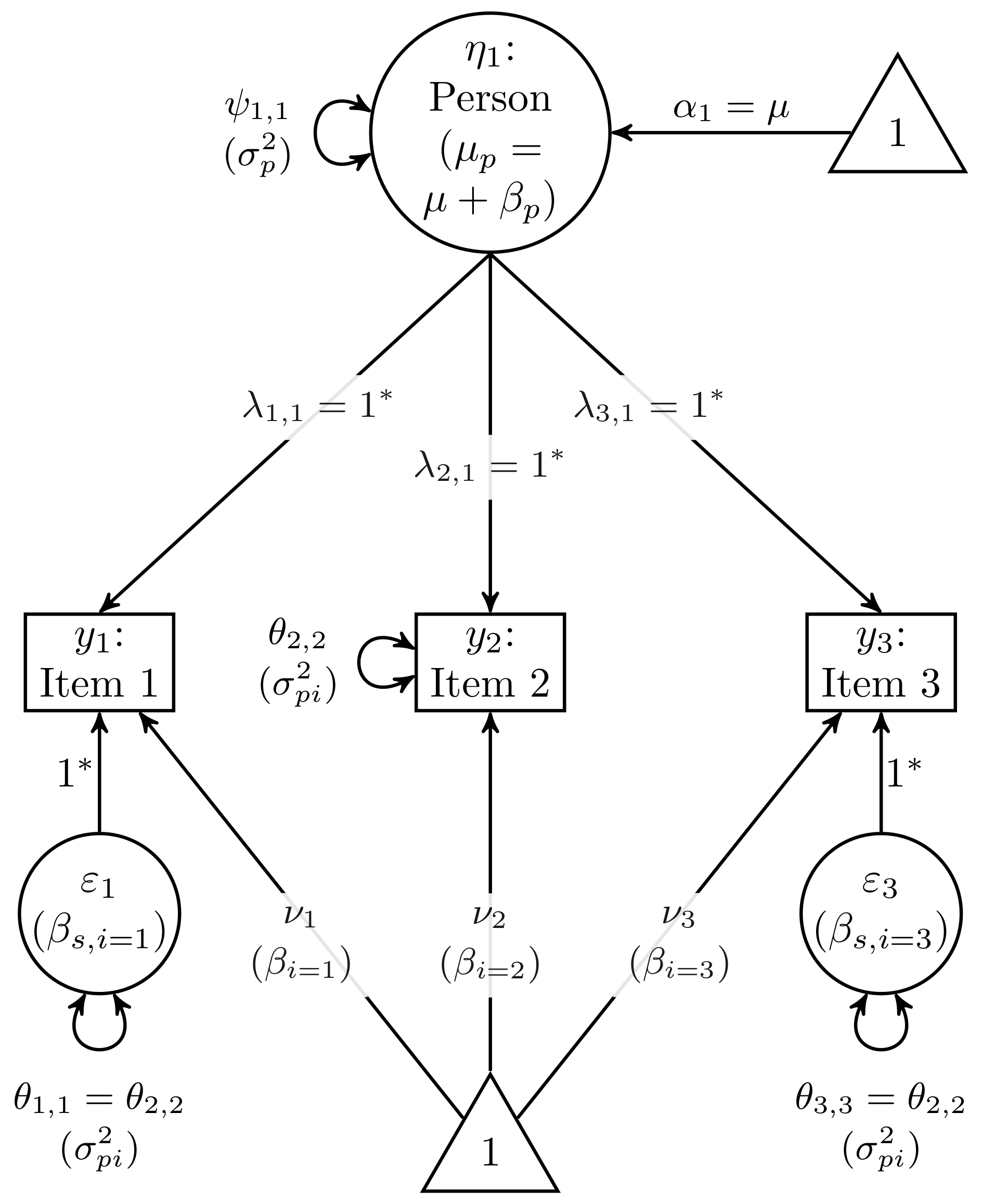
Figure 1. Path diagram depicting p × i GT model represented as a CFA with 3 indicators (items) as the facet of generalization. Each CFA variable and parameter are labeled using traditional LISREL notation, accompanied by GT notation in parentheses. The unique-factor variances are constrained to equality, the item intercepts are constrained to average zero to identify the factor mean (grand mean μ from GT), and the variance of intercepts represents the variance component σ i 2 (main effect of items). The unique factor for Item 2 is omitted for clarity, and its variance is instead depicted with a double-headed arrow pointing to Item 2 itself.
Psych 03 00011 g001
Figure 2. Two layers of a path diagram depicting a p × i × o GT design represented as a CFA model with 9 indicators (3 items × 3 occasions). Each CFA variable and parameter are labeled using LISREL notation, accompanied by GT notation in parentheses. Identification constraints on the mean structure are listed in Table 1. (a) The Person facet (of differentiation) is the first common factor. Residuals capture the highest-order term, confounded with any other source(s) of error. Intercepts of indicator residuals represent the interaction between all facets of generalization. (b) The facets of generalization interact with the Person facet (captured by the common factors), and their main effects are captured by the factor means.
Psych 03 00011 g002aPsych 03 00011 g002b
Figure 3. Path diagram depicting p × ( i : o ) GT model represented as a CFA with 9 indicators (items) across 3 occasions as facets of generalization. LISREL (and GT) notation are provided for each CFA variable and parameter. The Person facet (of differentiation) is the first common factor, and the p × o interaction is captured by Occasion factors, whose variances are constrained to equality. Residuals capture the highest-order term, confounded with any other source(s) of error, and their variances are constrained to equality. Identification constraints on the mean structure are listed in Table 1.
Psych 03 00011 g003
Figure 4. D-coefficients for cut-scores on ACP-CAT scale totals, using p × r data from Task 1, estimated with ML in lavaan (vs. REML in gtheory).
Psych 03 00011 g004
Table 1. Constraints required for mean-structure parameters to represent main and interaction effects among facets of generalization.
Latent InterceptIdentification Constraint p × i p × i × o p × ( i : o ) Ordinal
Person ( μ ) m = 1 n i × n o ν m = 0
Item 1 ( β i = 1 ) o = 1 n o β ( i = 1 ) , o = 0
Item 2 ( β i = 2 ) o = 1 n o β ( i = 2 ) , o = 0
Item 3 ( β i = 3 ) i = 1 n i β i = 0
Occasion 1 ( β o = 1 ) i = 1 n o β i , ( o = 1 ) = 0
Occasion 2 ( β o = 2 ) i = 1 n o β i , ( o = 2 ) = 0
Occasion 3 ( β o = 3 ) i = o n o β o = 0
First Measurement (LRV) c = 1 C τ c , ( m = 1 ) = 0
All other LRVs τ c , ( m > 1 ) = τ c , ( m = 1 ) , for each c = 1 , , C
Note. LRV = Latent response variable. The Person factor’s constraint is given in terms of indicator intercepts ( ν ) indexed by measurement m. Minor factors’ constraints are given in terms of GT effects ( β * , with i and o subscripts indexing items and occasions, respectively), which map onto SEM parameters as shown in path diagrams for each model (Figure 1, Figure 2 and Figure 3). Columns 3–5 indicate which constraints are required for each GT design. The rightmost column indicates which additional constraints are required when a CFA includes a threshold ( τ ) model to map each ordinal indicator with C + 1 categories onto a continuous LRV.
Table 2. Estimated generalizability and dependability coefficients for normal and discretized data under different estimators.
p × i p × i × o p × ( i : o )
DataResponse ScaleEstimatorGDD-CutGDD-CutGDD-Cut
NormalObservedMS0.8340.7830.9660.7370.6290.9560.7940.7280.970
REML0.8340.7830.9660.7370.6290.9560.7940.7280.970
ML0.8340.7820.9680.7370.6260.9590.7940.7120.969
Discretized MS0.7590.7060.9580.7150.6020.9580.7580.6910.970
REML0.7590.7060.9580.7150.6020.9580.7580.6910.970
ML(R)0.7590.7050.9600.7150.6000.9610.7580.6760.969
LRVDWLS0.8570.7920.9690.7730.6510.9600.8170.7300.970
Observed a 0.7810.7380.780
Note. LRV = latent response variable. MS = mean-squares estimates, manually calculated from R’s anova() output for linear model (lm) objects. REML = restricted maximum likelihood estimates, obtained from the R package gtheory (cut-score D-coefs must be calculated manually). ML(R) = maximum likelihood estimates (with robust S E s) obtained from the R package lavaan. DWLS = diagonally weighted least-squares estimates obtained from lavaan, interpreted on the latent response scale [17,18]. The 3 GT designs are labeled in the upper header, below which indicates columns with G-coefs, global D-coefs, and cut-score-specific D-coefs for that design. a Using IFA model parameters on the LRV scale, Green and Yang [48] incorporated thresholds to define reliability (equivalent to a G-coef) on the observed discrete response scale.
Publisher’s Note: MDPI stays neutral with regard to jurisdictional claims in published maps and institutional affiliations.