Heuristic and Metaheuristic Approaches for the Multi-Node Allocation Problem in Large-Scale IoT Networks

Abstract

The Multi-Node Allocation (MNA) problem in Internet of Things (IoT) networks arises when application requirements exceed the capacity of a single node, requiring job distribution across multiple devices. This problem is challenging in large-scale heterogeneous environments once it involves optimizing resource utilization, bandwidth consumption, and latency within a rapidly expanding search space. This paper proposes two scalable approaches: a greedy heuristic called Demand Index Multi-Node Allocation (DI-MNA) and a hybrid evolutionary algorithm (NSGA-Hyb) that combines DI-MNA with NSGA-III. Both methods use bounded combinatorial exploration and a normalized demand index to guide the search efficiently. The approaches are evaluated on IoT networks ranging from 10 to 1000 nodes under different workload conditions and compared with an optimal Branch and Bound (B&B) algorithm for small instances. Results show that DI-MNA achieves near-optimal solutions in small networks while maintaining low computational cost as network size grows. In large-scale scenarios, DI-MNA consistently matches or outperforms the evolutionary methods and sustains runtime speedups of up to $51\times$ over NSGA-Hyb and more than $7.8\times {10}^6$ over B&B. These findings demonstrate that DI-MNA provides an effective balance between solution quality, scalability, and computational efficiency for resource allocation in large-scale IoT networks.

1. Introduction

In an increasingly dense and demanding network landscape, adaptive, distributed, and quality-of-service (QoS)-oriented approaches have become essential to ensure the performance and reliability of Internet of Things (IoT) applications. A critical challenge for the viability of these environments is the efficient allocation of applications to the available resources [1,2].

The primary motivation for this work lies in the fact that modern application demands frequently exceed the individual processing, memory, and bandwidth capacities of a single sensing node or edge device. When application demands surpass local resource availability, the associated workload must be strategically distributed across multiple nodes, giving rise to the Multi-Node Allocation (MNA) problem. To keep the terminology consistent throughout the manuscript, the unit of allocation is hereafter termed a job: a job denotes the concrete, schedulable workload (characterized by its processing, bandwidth, and latency requirements) that the allocation algorithm must place on the network, whereas the term application is reserved for the higher-level IoT service whose requirements give rise to that job. The word task is used only when reproducing the terminology of prior work (e.g., “task offloading”, “task scheduling”) as named by the cited authors. While this process inherently involves network resource management, the primary focus of this paper is job allocation within a heterogeneous infrastructure of nodes, bandwidths, and latencies.

The optimal solution of the MNA problem is inherently complex, so the problem is NP-hard [3], as it involves structural network heterogeneity and the requirement for simultaneous optimization of multiple criteria, such as energy efficiency, scalability, and stringent QoS metrics. In large-scale IoT networks, optimal solution methods become computationally infeasible due to the required processing time. This limitation underscores the necessity for heuristics and metaheuristics capable of identifying high-quality solutions within feasible runtimes, thereby ensuring the adaptability required to maintain system reliability.

Informally, the MNA problem can be stated as follows. Given a heterogeneous IoT network of nodes, each characterized by an available processing capacity, an available bandwidth, and pairwise communication latencies, and given a set of jobs, each with its own processing, bandwidth, and latency requirements, the goal is to assign every job to a disjoint subset of nodes whose aggregated resources jointly satisfy that job’s requirements. Multi-node assignment becomes necessary precisely when no single node is sufficient to serve a job on its own, so that the demand must be met by combining the capacity of several cooperating nodes while still respecting the end-to-end latency deadline. The problem raises three intertwined research challenges. (i) Structural heterogeneity: nodes differ widely in capacity, so allocation quality depends on how well subsets of dissimilar nodes are composed. (ii) Competing objectives: processing, bandwidth, and latency pull the search in conflicting directions, and satisfying one criterion frequently degrades another, which makes the balance among the three the central difficulty. (iii) Combinatorial explosion: the number of candidate node subsets grows exponentially with the network size, rendering exact methods intractable. These three challenges expose a concrete gap in the literature: in Section 3, only one work addresses Multi-Node Allocation explicitly, and none demonstrates a scalable, near-optimal method on general (cyclic) IoT topologies at the scale of thousands to hundreds of thousands of nodes. Closing this gap is the direct motivation for the approaches proposed in this paper.

In this context, this paper addresses the MNA problem in large-scale IoT environments through a scalarized optimization model that concurrently considers resource consumption, bandwidth utilization, and latency. We present algorithmic approaches suitable for finding solutions in networks comprising thousands of nodes. The main novelty lies in the scale-aware normalization of multi-node Demand Index (DI) combined with bounded combinatorial exploration, enabling MNA under heterogeneous IoT constraints.

The research objectives of this work were threefold: (i) to formulate a scalarized MNA optimization model that jointly captures processing resources, bandwidth, and latency; (ii) to design a scalable heuristic that attains near-optimal allocations at a low and predictable runtime; and (iii) to validate and compare the heuristic to an exact baseline and evolutionary metaheuristics across a wide range of network sizes and workloads. The main contributions of this work are:

• A demand index-based greedy heuristic (DI-MNA) specifically tailored for job allocation on IoT resource-constrained networks.
• A standard (NSGA-Enh) and a hybrid (NSGA-hyb) metaheuristic approach. NSGA-Enh and NSGA-hyb are built on top of the NSGA-III [4] evolutionary algorithm.
• A comprehensive experimental analysis regarding performance and quality of the solutions in large networks and dense utilization scenarios, including benchmarking against optimal solutions to validate efficacy.

In this study, the adoption of the terms heuristics and metaheuristics and their categorization were based on [5]. DI-MNA is a heuristic, tailored for job allocation on resources of an IoT network, covering the combination of (a) a scale-aware, amplitude-normalized Demand Index that balances heterogeneous demands with (b) a bounded combinatorial search (hyperparameters $\alpha$, $\beta$) that keeps the method polynomial while still enabling genuine Multi-Node Allocation over cyclic topologies. NSGA-Enh is an evolutionary metaheuristic based on NSGA-III by adopting the best solution at each iteration. NSGA-Hyb is a hybrid metaheuristic, initializing NSGA-III with DI-MNA results to combine constructive efficiency and exploratory capacity, thereby enhancing convergence and solution quality. Henceforth, NSGA refers to NSGA-III (Non-dominated Sorting Genetic Algorithm III). To the best of our knowledge, no prior work delivers feasible MNA at the 10³–10⁵-node scale IoT networks with the runtime predictability presented in this paper.

2. Background

This section outlines the MNA problem in IoT networks, focusing on the challenges of selecting nodes for data processing and communication in constrained distributed environments. Heuristic and metaheuristic solutions are introduced as efficient strategies that iteratively make locally optimal decisions to generate viable solutions, although they do not ensure global optimality.

2.1. Multi-Node Allocation Challenges in IoT

The efficient allocation of applications (or jobs) within IoT environments is a fundamental challenge in designing intelligent distributed systems. IoT networks usually comprise heterogeneous devices, sensors, actuators, gateways, and edge servers, with varying computing, communication, and energy capabilities. This diversity requires allocation strategies that simultaneously account for multiple performance criteria [6].

The complexity of the problem increases when dealing with MNA, which refers to distributing a single application (or job) across multiple nodes in the network. Among the most critical resources involved in the allocation process are processing capacity (R), bandwidth (B), and latency (L). The allocation to multiple nodes can be useful and even necessary in scenarios where jobs can be partitioned, using parallel processing, partial offload, or to ensure redundancy and reliability [7].

The MNA problem is structurally analogous to the Generalized Facility Location Problem (GFLP) [8], in which multiple units of a “demand” can be simultaneously satisfied by various “facilities” (nodes), and the goal is to optimize the allocation in terms of cost, distance, and capacity. The optimal solution for the GFLP has exponential complexity due to the search space of the facilities. In the IoT context, some of the main challenges commonly related to MNA are presented as follows:

• Resource Heterogeneity: Resource heterogeneity represents a point of convergence between IoT networks and fog computing. In the context of the Internet of Things, this diversity is manifested in the varying capabilities of devices, such as processing power and memory, which makes task allocation a complex problem that requires optimizing the utilization of each node’s resources. Similarly, in fog computing architectures, the heterogeneity of computing and storage capacities across distributed devices necessitates the use of efficient algorithms to optimize service allocation and ensure optimal performance in metrics such as latency and resource utilization. Some studies [6,9] emphasize that, in distributed computing environments, heterogeneity is a key factor that demands the adoption of multi-objective optimization algorithms to achieve efficient and balanced resource management.
• Trade-off Between Latency and Resource Consumption: Applications such as autonomous vehicles, patient monitoring, and industrial systems require real-time responses. Reducing latency may require assigning job segments to nodes that are physically closer or have more available resources. However, this strategy can cause local overload, exceed available bandwidth, or compromise network stability. This scenario illustrates a classical optimization problem comprised of a set of functions in which it is required to balance the efficient usage of R, B, and L. It is not always possible to minimize all objectives simultaneously, thus the importance of the Pareto front, which represents the set of non-dominated solutions, i.e., those where improving one criterion necessarily degrades another [8,10].
• Scalability and Computational Complexity: Allocating jobs across multiple nodes is computationally more complex than single-node allocation. Given a network with n nodes and a job that can be partitioned into k subcomponents, the number of possible combinations grows exponentially. The problem is NP-hard, and exact solutions become infeasible for real-world networks. Heuristic and metaheuristic algorithms, such as NSGA, Ant-Colony Optimization (ACO), or MOPSO (Multi-Objective Particle Swarm Optimization), are often employed to approximate the Pareto front and provide multiple feasible solutions with different trade-offs among criteria [6,9,10].

2.2. Heuristic and Metaheuristics Methods for MNA in IoT

To address the complexity of the MNA problem, heuristic techniques have been widely adopted for their ability to provide feasible solutions while meeting appropriate runtime requirements. Prominent techniques include greedy algorithms, bin-packing heuristics, and linear relaxation methods with rounding [11,12,13]. These approaches are particularly effective in balancing trade-offs between limited resources and dynamic demands typical of distributed IoT environments [7,14]. Dynamic heuristic strategies that consider application priorities, runtime, and communication constraints have shown promising results in optimizing available resources, outperforming exact methods in terms of scalability and practical applicability in real-world scenarios [15].

The problem can also be efficiently modeled as an evolutionary optimization problem, where each feasible solution is an individual and the set of solutions is a population. In the evolutionary model, an individual represents a complete solution to the problem, that is, a specific assignment of all jobs to the available nodes. Each individual is composed of multiple genes, each gene encoding the allocation of a single job. The population consists of a variety of distinct individuals, each representing a feasible alternative to job allocation. This diversity allows evolutionary algorithms, such as the NSGA, to explore the search space broadly, promoting the continuous evolution of solutions through selection, crossover, and mutation operators. Mutation and crossover are essential operators in evolutionary algorithms, as they enhance population diversity, prevent premature stagnation, and enable efficient exploration of the search space, thereby fostering the attainment of higher-quality solutions [16,17].

3. Related Work

This section presents related studies, discussing methodologies, results, and contributions from the literature to contextualize and compare with the work proposed in this paper.

Fereira et al. [18] presented an Integer Linear Programming (ILP)-based framework for optimizing task allocation in distributed IoT environments (edge–fog–cloud), aiming to minimize the number of active nodes while meeting QoS constraints such as latency, bandwidth, and computational capacity. The framework was evaluated on a 15-node mesh network. The approach showed effectiveness, potentially decreasing node usage by about $9\%$, though it encountered scalability challenges for real-time applications. We highlight that the authors’ framework targets single-node selection through integer programming and is therefore conceptually and algorithmically distinct from the DI-MNA.

The authors in [19] proposed three heuristics to optimize task allocation in real-time IoT networks, focusing on reducing energy consumption. The approaches included a standard genetic algorithm (GA), a modified GA based on latency, and a delay-based mechanism that prioritized task allocation to nodes with shorter response times. The delay-aware algorithm demonstrated superior performance in latency-sensitive scenarios, achieving task allocation in less than 1 millisecond, while the modified GA showed enhanced scalability and faster convergence. The three heuristics reduced energy consumption by at least $37\%$ while fully satisfying QoS constraints such as latency, connectivity, and resource availability.

The approach in [20] introduces a novel evolutionary algorithm based on multi-objective optimization to enhance Internet of Everything (MO-IoE) services, optimizing conflicting metrics such as service time, workload, energy consumption, and latency. The proposed technique is a modified version of the Multi-Objective Differential Evolution (MODE) algorithm, incorporating an adaptive fast mutation operator and Pareto-based strategies to handle multi-objective problems, along with non-dominated sorting to maintain population diversity. The results demonstrate that the algorithm outperforms state-of-the-art methods such as Multi-Objective Particle Swarm Optimization (MOPSO) [21,22], Multi-Objective Whale Optimization Algorithm (MOWOA) [23,24], and Artificial Bee Colony Optimization (ABCO) [25,26], significantly reducing energy consumption, latency, and workload in IoE scenarios while also extending sensor lifetime.

The study presented in [27] conducts a systematic review and comparative analysis of metaheuristic algorithms applied to task offloading in distributed computing environments. The study evaluates categories such as evolutionary algorithms (e.g., genetic algorithm (GA), Non-dominated Sorting Genetic Algorithm II (NSGA-II)), swarm intelligence techniques (e.g., Particle Swarm Optimization (PSO), Ant Colony Optimization (ACO), Grey Wolf Optimizer (GWO), Whale Optimization Algorithm (WOA)), simulated annealing (SA), as well as hybrid approaches (e.g., GA-PSO) and approaches tailored for dynamic and security-sensitive scenarios. The results indicate that GA and PSO are particularly effective in optimizing resource usage and minimizing latency, while WOA and GWO provide a balanced trade-off among cost, energy consumption, and latency. ACO demonstrates strong performance in load balancing within complex networks. Practical implementation is deemed feasible in $84\%$ of the cases, with specific adjustments leading to up to $40\%$ savings in power consumption (GA-PSO) and $80\%$ improvement in hit rate through dynamic reconfiguration. That systematic review grounds the breadth of the metaheuristic landscape and provides the practical-feasibility and energy-saving figures reported across the GA, PSO, WOA, GWO, and ACO families.

The authors in [28] propose a task scheduling algorithm for edge computing environments that simultaneously addresses runtime, energy consumption, and load balancing among nodes. The method is based on a multi-objective optimization approach with weighted factors assigned to these three criteria, employing an adaptive bidding model in which tasks act as bidders and edge nodes as invitees, enabling the allocation of subtasks across multiple nodes (MNA). The experimental results demonstrate a $6.6\%$ reduction in task completion time, lower overall energy consumption, performance-compatible runtime with edge devices (on the order of microseconds), and low memory usage.

Taleb et al. [29] provide a structured and comprehensive overview of research concerning the Service Placement Problem (SPP) within integrated cloud–fog–edge environments. The authors introduce a novel classification of placement approaches from an algorithmic perspective, categorizing them into three primary frameworks: graph-based, heuristic, and machine learning.

Although related work [18,19,20,27] propose advances in resource optimization for IoT networks, most still focus on the assignment of tasks to single nodes, emphasizing energy consumption, latency, and computational usage. The only study identified so far that explicitly addresses MNA is [28], which optimizes resource usage by applying criteria such as runtime, energy consumption, and load balancing among nodes in dynamic environments. Nevertheless, significant gaps persist in the literature regarding the development of cooperative, scalable, and robust solutions for IoT applications. In this context, the heuristics proposed in this work perform a thorough exploration of node combinations, achieving predictability, reliability, and resilience, particularly in heterogeneous and resource-constrained IoT networks.

Table 1. Analysis of algorithms, layers, and metrics in the provided literature.

Ref	Date	Algorithm	Layer(s)	Metrics
[18]	2022	ILP	Edge, Fog	Latency, Bandwidth, Resource, Cost
[19]	2025	NSGA-II	Edge, fog, cloud	Energy, delay, reliability
[20]	2022	MO-IoE (evolutionary)	IoT, cloud	Delay, cost, throughput
[22]	2023	MOPSO	Fog, cloud	Latency, network throughput
[24]	2023	WOA	Edge, cloud	Energy efficiency, QoS
[26]	2024	ABC	Edge, serverless	Delay, execution cost
[27]	2025	Metaheuristics (survey)	Edge, fog, cloud	Delay, energy, cost, reliability
[28]	2020	NSGA-II	Edge	Time, energy, load balancing
[29]	2025	Heuristics, metaheuristics	Edge, fog, cloud	Latency, energy, costs, QoS, resources

presents a summary of recent research on node selection optimization in multi-layered IoT architectures, covering works published between 2020 and 2025, and reflects a growing interest in distributed resource management across heterogeneous infrastructures. The surveyed studies reveal a strategic distribution of computational tasks across the spectrum, from edge and network fog layers to cloud and serverless environments, with most works adopting hybrid layer configurations, such as edge–fog, fog–cloud, and edge–fog–cloud, highlighting the trend toward hierarchical infrastructures in large-scale IoT deployments. A wide range of algorithmic paradigms is identified, ranging from exact methods such as Integer Linear Programming (ILP) to metaheuristics and evolutionary frameworks, including NSGA-II, MOPSO, Artificial Bee Colony (ABC), and Whale Optimization Algorithm (WOA); among these, multi-objective evolutionary algorithms appear recurrently, underscoring their established role in handling the competing objectives inherent to IoT resource allocation, while heuristic and hybrid heuristic–metaheuristic approaches also emerge as practical alternatives for scalable and low-overhead solutions. These approaches are tailored to solve multi-objective optimization problems, balancing conflicting performance indicators such as latency, energy consumption, operational costs, reliability, throughput, and Quality of Service (QoS), where the diversity of metrics across studies reflects the multifaceted nature of IoT service placement and reinforces that no single objective suffices to characterize solution quality. Collectively, the reviewed works establish the algorithmic and architectural foundations upon which the present study builds, motivating the development of the DI-MNA heuristic and its NSGA-III-based metaheuristic extensions for large-scale Multi-Node Allocation in IoT networks. Table 1 is organized to foreground the most recent (2023–2025) and most directly comparable multi-node and hybrid heuristic–metaheuristic approaches.

The methodology adopted here also connects to a broader and long-standing body of combinatorial-optimization research, most notably the design and scheduling of multi-product batch plants. That problem is, like MNA, an NP-hard, resource-constrained allocation problem, and it has historically been approached using exact branch-and-bound (B&B), mixed-integer programming, and metaheuristics (ACO, genetic algorithms, and simulated annealing) [5]. Our experimental design has a B&B baseline algorithm playing the same ground-truth role as the B&B/MILP formulations used for optimal batch-plant scheduling, while our NSGA-III-based metaheuristics are the counterpart of the population- and swarm-based methods applied when the batch-plant search becomes intractable. The batch-plant literature has likewise devoted substantial effort to the efficient parallelization of both exact and approximate solvers. These strategies map naturally onto DI-MNA: its inner loop, which enumerates and evaluates candidate node combinations for each job, can be parallelized, so partitioning the job stream and the combination enumeration across workers is straight for the parallel versions of DI-MNA identified as future work (Section 6 and Section 7).

4. Optimization Model and Heuristics

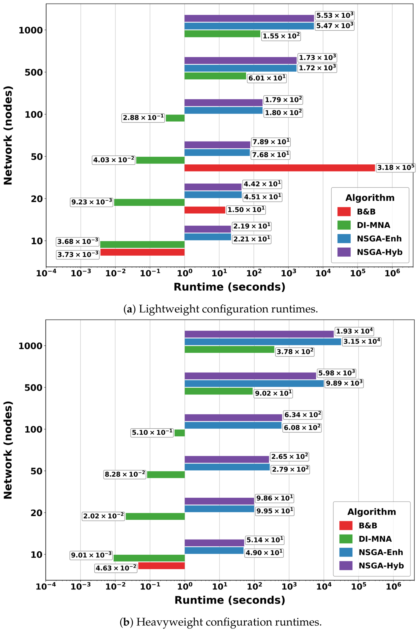
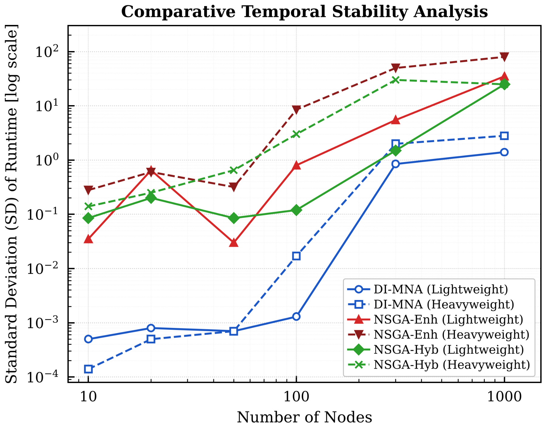
This section presents the optimization model for MNA, followed by three proposed heuristics. The first approach is a greedy method named Demand Index Multi-Node Allocation (DI-MNA), which employs a demand-based sequential strategy that considers resource, latency, and bandwidth constraints. The second is a heuristic based on the NSGA evolutionary metaheuristic, which explores the solutions’ search space and identifies non-dominated trade-off solutions. The third heuristic is a hybrid method combining the outcomes of DI-MNA with the generations of the NSGA metaheuristic.

4.1. Scalarized Optimization Model for MNA

The Multi-Node Allocation (MNA) problem consists of identifying groups of IoT nodes capable of jointly satisfying the computational and communication requirements of an application while respecting latency constraints. Unlike conventional placement approaches that associate each application with a single execution node, the MNA formulation allows the aggregation of resources from multiple devices whenever the demand of a job exceeds the capacity available at an individual node. To support the evaluation of alternative allocations, the problem is represented as a constrained optimization model in which candidate solutions correspond to combinations of nodes selected from the network. The objective is to identify feasible allocations that balance resource utilization efficiency and communication performance while avoiding unnecessary overprovisioning.

Table 2. Modeling assumptions between MNA-IoT [7] and the present work (DI-MNA).

Model Assumption	MNA-IoT [7]	This Work (DI-MNA)	Impact on Comparability
Layer architecture	Single edge layer	Single edge layer	Both studies adopted one single layer network.
Node availability	All nodes active	All nodes active	Both studies adopted all network nodes available for job placement.
Network topology	Tree (no cycles)	General graph (cycles allowed)	Cycle support enables fault-tolerant mesh topologies, common in large-scale IoT networks.
Job ordering	Not applied	Demand Index (DI), descending order	Prioritizes higher-demand jobs, reducing resource conflicts in early allocation iterations.
Search starting point	Any node (unconstrained)	Any node + pruning hyperparameters ($\alpha$, $\beta$)	Pruning accelerates the search for solutions in networks of 1000 nodes without significant loss of solution quality.

summarizes the modeling assumptions adopted in this study and highlights the main differences with respect to previous MNA formulations. These assumptions establish the operational boundaries of the optimization problem and the network setup.

The IoT infrastructure is represented by a weighted undirected graph $G=(V,E)$, where vertices represent edge devices and edges represent communication links between neighboring nodes. Each node $v\in V$ is characterized by its available processing capacity $f_r\left(v\right)$ and available bandwidth capacity $f_b\left(v\right)$. The weight associated with each edge corresponds to the one-way communication delay between the connected devices. 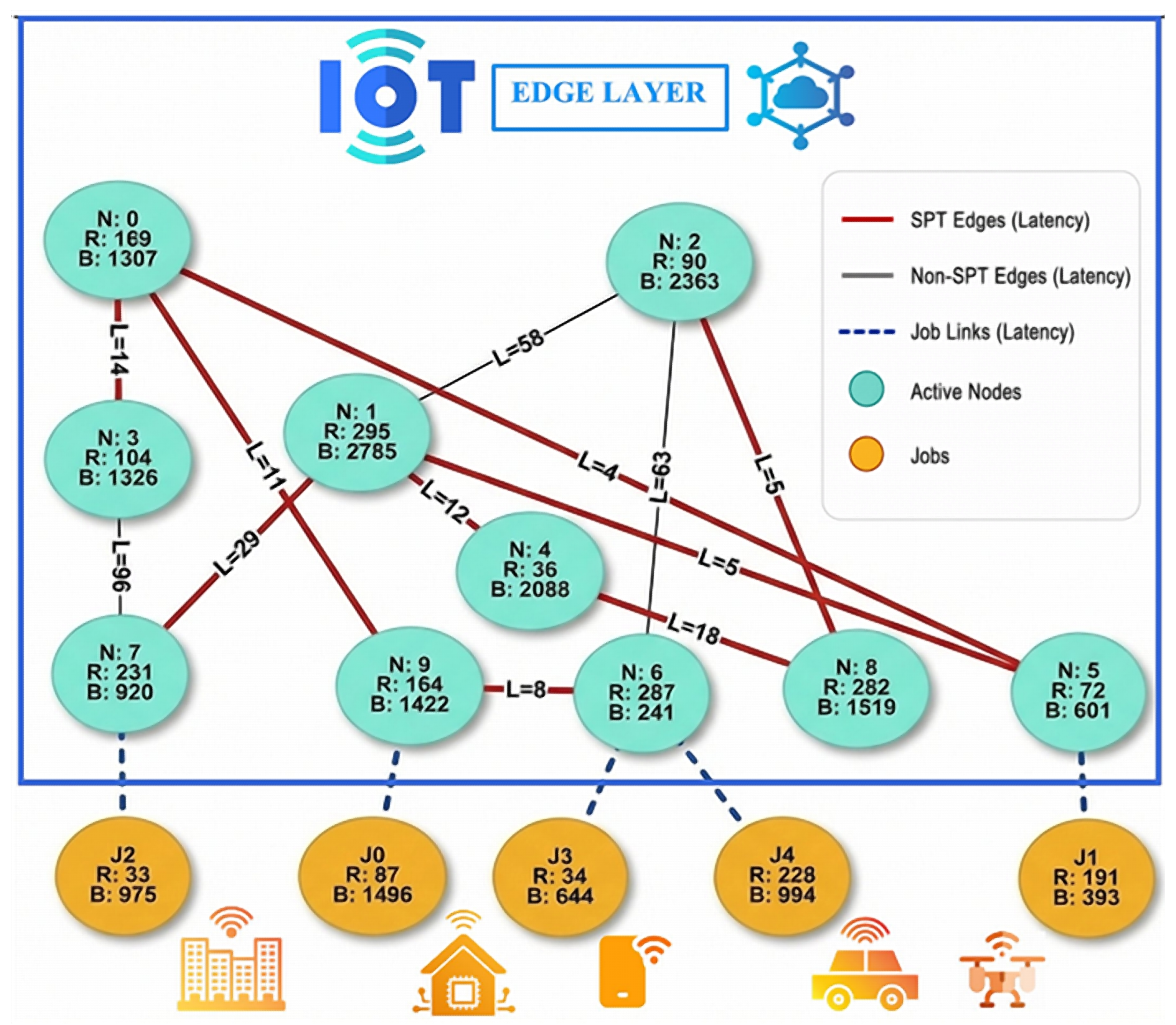Figure 1 presents an illustrative example containing ten nodes and five jobs. The network nodes are depicted as teal circles, each labeled with three attributes: N (node index), R (available resources), and B (available bandwidth). Jobs are represented as orange circles carrying analogous attributes—their index ($J_i$), R (required resources), and B (required bandwidth). Dashed blue lines (job links) connect each job to its associated edge node, indicating the communication latency between a given IoT application and its entry point into the network. The highlighted links (red edges) illustrate a shortest-path tree (SPT) rooted at a reference node and computed using Dijkstra’s algorithm over the one-way latency associated with each communication link. In this structure, every node reaches the root through its minimum-latency path, and the union of these paths forms the primary low-latency communication backbone of the topology. The remaining links (gray edges) are preserved to provide routing flexibility and increase connectivity, allowing multiple communication alternatives to coexist within the same topology. Because the network is modeled as a general graph, multiple routes may exist between two nodes. Consequently, the latency associated with a candidate allocation is obtained by applying Dijkstra’s algorithm to compute the shortest communication path between the selected nodes, where edge weights represent the one-way communication delay of each network link. The resulting latency therefore corresponds to the minimum cumulative delay among all feasible routes.

Because the network is modeled as a general graph, more than one route may exist between two nodes. Communication delays are determined by means of Dijkstra’s algorithm, which computes the least-cost path in a weighted graph representing the network topology. Consequently, the latency associated with a candidate allocation corresponds to the minimum cumulative delay obtained across all viable routes connecting the selected nodes, where edge weights represent the individual communication delays of each network link. Each candidate solution is evaluated through the scalarized objective function defined in Equation (1). The formulation combines processing resources, communication bandwidth, and latency into a single optimization criterion, thereby enabling direct comparison among candidate allocations.

$$\min F_R^2\left(i\right)+F_B^2\left(i\right)-F_L\left(i\right),\forall i=1,\dots ,n_{\mathrm{elem}}$$

(1)

where $n_{\mathrm{elem}}=2^{n_{\mathrm{nodes}}}$ denotes the total number of node combinations that compose the search space. The terms $F_R\left(i\right)$ and $F_B\left(i\right)$ quantify the excess processing and bandwidth capacities available after satisfying the requirements of a job, whereas $F_L\left(i\right)$ measures the remaining latency margin between the maximum tolerated delay and the communication latency observed for the allocation. The resource, bandwidth, and latency components are computed according to Equations (2)–(4).

$$F_R\left(i\right)={\displaystyle \sum _{k=1}^{n_{\mathrm{nodes}}}}{f}_r\left(k\right)-J_r\left(j\right),\forall j=1,\dots ,nj$$

(2)

$$F_B\left(i\right)={\displaystyle \sum _{k=1}^{n_{\mathrm{nodes}}}}{f}_b\left(k\right)-J_b\left(j\right),\forall j=1,\dots ,nj$$

(3)

$$F_L\left(i\right)=J_l\left(j\right)-f_l\left(i\right),\forall j=1,\dots ,nj$$

(4)

In these expressions, j denotes a job, k denotes a network node, and i identifies a candidate allocation. The parameters $J_r\left(j\right)$, $J_b\left(j\right)$, and $J_l\left(j\right)$ correspond to the processing, bandwidth, and latency requirements of job j, respectively. Likewise, $f_r\left(k\right)$ and $f_b\left(k\right)$ represent the processing and bandwidth capacities available at node k, while $f_l\left(i\right)$ denotes the cumulative latency associated with allocation i. The quadratic terms applied to $F_R\left(i\right)$ and $F_B\left(i\right)$ increase the cost assigned to allocations with excessive resource reservation, encouraging solutions that satisfy application demands with minimal surplus capacity. Conversely, the subtraction of $F_L\left(i\right)$ favors allocations that preserve larger latency margins and therefore provide greater tolerance to communication delays. A candidate solution is considered feasible only if all application requirements are simultaneously satisfied. The viability conditions are established by the constraints represented in (5):

$$F_R\left(i\right)\ge 0,F_B\left(i\right)\ge 0,F_L\left(i\right)\ge 0,\forall i=1,\dots ,n_{\mathrm{elem}}$$

(5)

ensuring that sufficient processing resources and bandwidth are available while maintaining the end-to-end delay within the latency limit specified by the application.

Operational interpretation of the objective. Each term of Equation (1) maps to a concrete performance dimension of edge-IoT allocation. The term $F_R\left(i\right)$ is the surplus processing capacity left after satisfying a job; squaring it penalizes over-provisioning super-linearly, steering the heuristic toward tight resource utilization and away from reserving powerful nodes for small demands (efficient consolidation). The term $F_B\left(i\right)$ is the analogous surplus bandwidth capacity and is treated symmetrically, since bandwidth is a first-class scarce resource in dense IoT deployments. The term $F_L\left(i\right)$ is the latency margin between the maximum tolerated delay and the end-to-end delay of the chosen route (computed via Dijkstra’s algorithm); it is subtracted so that, among equally resource-efficient allocations, those preserving larger latency headroom are preferred, directly improving QoS robustness for latency-sensitive applications.

Rationale for minimizing this metric. The formulation encodes the central engineering trade-off of MNA: satisfying demand with the minimum necessary surplus (tight utilization) while retaining the maximum feasible latency margin (QoS safety). The quadratic penalties on R and B express a diminishing tolerance for waste, whereas latency is enforced as a hard feasibility constraint (Equation (5)) rather than a soft objective. Minimizing surplus resource and bandwidth reservation is also a widely used and well-motivated proxy for operational and energy cost, since idle-but-reserved capacity corresponds to under-utilized and energy-consuming infrastructure; consolidating jobs onto fewer, better-matched nodes is the mechanism by which the literature relates utilization to energy and cost efficiency. Energy is not modeled as an explicit term in the present objective; incorporating an explicit energy-consumption term is identified as a planned extension in Section 7.

Complexity Characterization

The intractability of MNA was motivated in Section 2.1 by its structural analogy with the GFLP. This subsection makes that claim rigorous by identifying the classical problems from which MNA is reduced and exhibiting them as special cases of the model. Making the source problem explicit lets us replace a bespoke argument with the standard restriction technique: we show that Subset-Sum and its exact-partition strengthening 3-Partition are special cases of MNA, which yields ordinary and strong NP-hardness, respectively. We first state the decision problem and then present the two reductions, their correctness, and a generalization argument.

Decision version (Mna-Dec). Given a set of nodes with processing capacities $\left\{f_r\left(k\right)\right\}$ and bandwidth capacities $\left\{f_b\left(k\right)\right\}$, an inter-node latency structure, a set of jobs with demands $\{J_r\left(j\right),J_b\left(j\right),J_l\left(j\right)\}$, and a bound $\kappa$, Mna-Dec asks whether there exists a feasible allocation whose objective value (Equation (1)) is at most $\kappa$. A feasible allocation assigns a node-disjoint subset to each job that satisfies the resource, bandwidth, and latency constraints of the model ($F_R,F_B,F_L\ge 0$, Equation (5)). Since such an allocation is a certificate verifiable in polynomial time, $\mathrm{M}\mathrm{N}\mathrm{A}\text{-}\mathrm{D}\mathrm{E}\mathrm{C}\in \mathrm{NP}$.

Source problem and single-job reduction (Subset-Sum). In Subset-Sum, given a multiset $S=\{a_1,\dots ,a_m\}$ of non-negative integers and a target T, the problem asks whether some sub-multiset of S sums exactly to T. From an arbitrary instance, we construct, in $O\left(m\right)$ time, an Mna-Dec instance as follows:

• Create m nodes with processing capacities $f_r\left(k\right)=a_k$, $k=1,\dots ,m$;
• Make the bandwidth and latency dimensions vanish identically: set $f_b\left(k\right)=0$ for every node and $J_b=0$ for the job, and set all link latencies (hence the route latency $f_l$) and $J_l$ to 0; then, $F_B\equiv 0$ and $F_L\equiv 0$ for every node subset, so both constraints $F_B,F_L\ge 0$ hold with equality, and neither term contributes to the objective;
• Create a single job with $J_r=T$;
• Set the objective bound $\kappa =0$.

Correctness. Because $F_B\equiv 0$ and $F_L\equiv 0$, the objective of Equation (1) reduces exactly to $F_R^2={\left({\sum }_{k\in \mathcal{A}}{f}_r\left(k\right)-T\right)}^2$ for the chosen subset $\mathcal{A}$. Feasibility ($F_R\ge 0$) requires ${\sum }_{k\in \mathcal{A}}{f}_r\left(k\right)\ge T$, and since a square is non-negative, this value is at most $\kappa =0$ if and only if ${\sum }_{k\in \mathcal{A}}{f}_r\left(k\right)=T$ exactly, i.e., if and only if the Subset-Sum instance is a Yes instance. The construction is polynomial, hence Subset-Sum ≤_p Mna-Dec; with membership in NP, Mna-Dec is NP-complete and MNA is NP-hard.

Strong NP-hardness (3-Partition). The single-job core is only weakly NP-hard, since Subset-Sum admits a pseudo-polynomial algorithm. The multi-job problem is strictly harder. Recall that 3-Partition asks whether $3m$ positive integers $a_1,\dots ,a_{3m}$, each with $a_i\in (B/4,B/2)$ and ${\sum }_i{a}_i=mB$, can be partitioned into m triples each summing to B; it is strongly NP-complete. Construct an Mna-Dec instance with $3m$ nodes of capacity $f_r\left(k\right)=a_k$, m jobs each with demand $J_r=B$, the bandwidth and latency dimensions made to vanish as above, and $\kappa =0$. Since the total capacity $mB$ equals the total demand $mB$ and the m allocations are node-disjoint with each $F_R\ge 0$, every node must be used and each job must receive nodes summing to exactly B; the surplus objective ${\sum }_j{\left({\sum }_{k\in {\mathcal{A}}_j}{f}_r\left(k\right)-B\right)}^2$ attains $\kappa =0$ precisely in this case. The bounds $a_i\in (B/4,B/2)$ force each job to receive exactly three nodes. Hence, the instance is a Yes instance if and only if the $a_i$’s admit an exact 3-partition, giving 3-Partition ≤_p Mna-Dec. As 3-Partition is strongly NP-complete, MNA is strongly NP-hard and admits no pseudo-polynomial-time algorithm unless $\mathrm{P}=\mathrm{NP}$.

Generalization. These two restrictions place MNA within the classical hierarchy Subset- Sum ⊆ (Multiple-)Knapsack/Bin-Packing ⊆ Mna, with 3-Partition supplying strong hardness at the multi-job level. With multiple jobs and the node-disjointness (no-sharing) requirement, MNA contains Multiple-Knapsack and Bin-Packing as special cases, both NP-hard, while the bandwidth and latency constraints and the quadratic surplus penalty can only add difficulty. This formally justifies the intractability previously supported only by the GFLP analogy and, in turn, motivates the heuristic and metaheuristic approaches developed in the remainder of this section.

4.2. A Demand Index Multi-Node Allocation Heuristic

The work presented in [7] aimed at allocating jobs across multiple nodes while minimizing resource waste and satisfying application latency constraints. Despite its capability to perform multi-node job allocation, the MNA-IoT heuristic exhibits several limitations: (a) no job ordering mechanism is employed prior to the allocation process—in contrast to the Demand Index (DI) adopted in DI-MNA (Equation (6)), which demonstrated effectiveness in prioritizing higher-demand jobs and contributed to improved solution quality—and the absence of such an ordering strategy may significantly impact overall system performance, particularly in sequential or real-time execution contexts; (b) the network topology is required to follow a tree structure, thereby precluding the presence of cycles.

We propose a Demand Index–based Multi-Node Allocation (DI-MNA) heuristic designed to address the limitations of the previous MNA-IoT approach by more effectively accommodating the highly variable demands of jobs and by mitigating allocation bias toward any individual parameter ($R,B$, L). The direct methodological predecessor of DI-MNA is the authors’ own MNA-IoT heuristic [7];

Table 3. Conceptual, architectural, algorithmic, and functional differences between DI-MNA and its direct predecessor heuristic MNA-IoT [7].

Dimension	Predecessor MNA-IoT [7]	This Work (DI-MNA)—Innovation
Conceptual	No job ordering; allocation order is arbitrary.	An amplitude-normalized, scale-aware Demand Index orders jobs by demand, reducing resource conflicts in the early allocation iterations.
Architectural	Requires a tree topology (no cycles).	Operates over a general graph (cycles allowed), enabling fault-tolerant mesh topologies through a Dijkstra-based shortest-path-tree (SPT) backbone plus redundant edges.
Algorithmic	Unrestricted/unbounded candidate search.	Bounded combinatorial search with pruning hyperparameters $\alpha ,\beta$ and polynomial complexity $O\left(J{V}^{\beta }\right)$.
Functional	Single-instance heuristic, limited scale.	Validated from 10 to 100,000 nodes, compared against the exact B&B optimum and NSGA-III variants, and a statistical stability analysis.

contrasts DI-MNA with its predecessor [7] along four dimensions.

These differences are not an incremental tuning of parameters: the Demand Index normalization, the generalization from trees to arbitrary graphs, and the complexity guarantee of the bounded search together constitute the central methodological novelty, and they are precisely what enables near-optimal MNA at scales far beyond the predecessor.

The new demand index ensures that jobs’ demand variables with larger amplitudes are properly balanced. Equation (6) presents the Demand Index (DI) regarding the processing resources (R), bandwidth (B), and latency (L) demands of each job:

$$\mathrm{DI}=c_0^{\prime }R+c_1^{\prime }B-c_2^{\prime }L$$

(6)

Coefficients $c_i^{\prime },i=\{0,1,2\}$, are applied to balance each variable. The coefficients use a common scale factor and are calculated according to the expression in Equation (7):

$$c_i^{\prime }={\displaystyle \frac{\frac{1}{\mathrm{amp}\left(X_i\right)}}{{\sum }_{j=0}^2\frac{1}{\mathrm{amp}\left(X_j\right)}}}·w_i,\mathrm{where}{\displaystyle \sum _{i=0}^2}{w}_i=1$$

(7)

where $X_0=R$, $X_1=B$, and $X_2=L$ denote, respectively, the computational resource capacity, available bandwidth, and end-to-end latency associated with each IoT node. The amp function computes the amplitude of the domain of each decision variable, defined as the difference between its upper and lower bounds. The weighted coefficients $w_i$ were empirically determined to compensate for scale disparities among the variables and to mitigate distortions introduced by heterogeneous amplitude ranges. These weights are constrained to sum to unity, thereby ensuring a normalized contribution of all objectives within the optimization framework. This normalization prevents decision variables with larger domains, such as bandwidth when compared to latency, from disproportionately influencing the search process, improves convergence behavior in evolutionary multi-objective algorithms (e.g., NSGA-III), and facilitates the handling of constraints and penalty functions in the optimization process.

After calculating the DI for each job, the heuristic sorts the jobs in descending order (array J). Then, there is a greedy search over the nodes’ space that systematically evaluates all feasible node combinations. For each job, the aggregated resource capacity, bandwidth, and latency of each combination are computed and evaluated using an optimization function that minimizes surplus resource and bandwidth while maximizing the remaining latency margin.

The heuristic processes each job by applying the stages of preliminary node selection, search space generation, and solution evaluation. For each feasible solution, an objective function is computed to minimize resource overuse and cumulative latency. The best solution is then selected, and the corresponding nodes are marked as unavailable for future allocations.

The DI-MNA heuristic is summarized in Algorithm 1. The algorithm inputs are the arrays of resource capacity (R), bandwidth (B), and latency (L) of the network, along with arrays of job demands: processing ($J_r$), bandwidth ($J_b$), and latency ($J_l$). Each job originates from a specific node ($J_o$), and the network connections (edges) are represented in an adjacency list ($adjList$). Hyperparameters $\alpha$ (cut_comb_nodes) and $\beta$ (cut_sol) provide, respectively, an upper bound on the number of available node combinations and the maximum number of nodes in a solution for a given job. These parameters set the bounds of the search space for feasible node combinations, thereby reducing the runtime of the heuristic.

Line 1 shows the connection time of each job to the node ($t_c=1$). In line 2, all nodes are initially marked as available. The DI index is calculated according to the coefficients $c_0^{\prime }$, $c_1^{\prime }$, and $c_2^{\prime }$ (line 3), and the list of jobs (J) is sorted in descending order (line 4). The algorithm then iterates over each job $j\in J$ (line 5), processing them sequentially.

For each job, the latencies of the nodes relative to the source $J_o\left[j\right]$ are computed using Dijkstra’s algorithm (line 6). Next, a subset of candidate nodes is preselected (line 7) according to a latency threshold criterion and basic constraints imposed by the hyperparameters $cut\_comb\_nodes$ and $cut\_sol$. The best solution found ($bestsolution$) is also initialized as empty, and its objective function value $Min\_FX$ is set to the highest value (line 8), ensuring that any feasible solution is considered as an improvement.

The algorithm examines all possible combinations of nodes within the filtered set, provided that they respect the maximum size limit $\beta$ (line 9). For each candidate combination $comb\_nodes$, the aggregated resources $(Su{m}_R,Su{m}_B,Su{m}_L)$ are computed (line 10). If the combination meets the job requirements—namely, processing resources ($Su{m}_R\ge J_r\left[j\right]$), bandwidth ($Su{m}_B\ge J_b\left[j\right]$), and latency ($Su{m}_L\le J_l\left[j\right]-t_c$) (line 11)—then the objective function is evaluated (lines 12–13). The objective function ($OF$) balances two factors: minimizing the overprovisioning of resources and bandwidth while maximizing the latency slack. Whenever the computed $OF$ value is lower than the current best value ($Min\_FX$), the best solution is updated (line 13).

After evaluating all combinations (lines 9–16), the algorithm verifies whether a feasible solution has been found (line 17). If so, the selected nodes are allocated and marked as unavailable (line 18) to prevent their reuse in subsequent jobs. The objective function value and the set of allocated nodes are then recorded (line 19). Otherwise, the algorithm stores an empty allocation and assigns zero to the objective function (line 21).

Algorithm 1 DI-MNA heuristic.

Inputs: Resources: $R,B,L$; job demands: $J_r,J_b,J_l,J_o$; coefficients: $c_0^{\prime },c_1^{\prime },c_2^{\prime }$; adjacency list: $adjList$; hyperparameters: $cut\_comb\_nodes\leftarrow \alpha$, $cut\_sol\leftarrow \beta$; Outputs: Allocated nodes: $v\_all\_nodes$; OF values: $v\_all\_OF$   1: $t_c\leftarrow 1$    % connection time (ms)   2: $available\leftarrow [\mathrm{True},\dots ,\mathrm{True}]$   3: $\mathrm{DI}=c_0^{\prime }R+c_1^{\prime }B-c_2^{\prime }L$   4: $J=list(\ast ordered\_list(DI\left)\right)$   5: for all job j in J do   6:     Compute node latencies from source $J_o\left[j\right]$ using Dijkstra   7:     $filtered\_nodes\leftarrow$ Preselect based on latency threshold   8:     Initialize $Min\_FX\leftarrow \infty$, best solution $\leftarrow \varnothing$   9:     for all node subsets $comb\_nodes\subseteq filtered\_nodes$            with size $\le cut\_sol$ do 10:           Resource computation $(Su{m}_R,Su{m}_B,Su{m}_L)$ 11:           if job requirements satisfied: $Su{m}_R\ge J_r\left[j\right]$,             $Su{m}_B\ge J_b\left[j\right],Su{m}_L\le J_l\left[j\right]-t_c$ then 12:              Compute $OF\leftarrow {(Su{m}_R-J_r\left[j\right])}^2+$            ${(Su{m}_B-J_b\left[j\right])}^2-(J_l\left[j\right]-t_c-Su{m}_L)$ 13:              if $OF<Min\_FX$ then update best solution 14:              end if 15:           end if 16:       end for 17:      if best solution found then 18:           Allocate nodes and set them unavailable 19:           Store $Min\_FX$ and allocated nodes 20:      else 21:           Store 0 and empty allocation 22:      end if 23: end for

This procedure is repeated for all jobs, ensuring that each one is individually evaluated and that network resources are allocated consistently. No node sharing is allowed, while always respecting latency, resource, and bandwidth constraints.

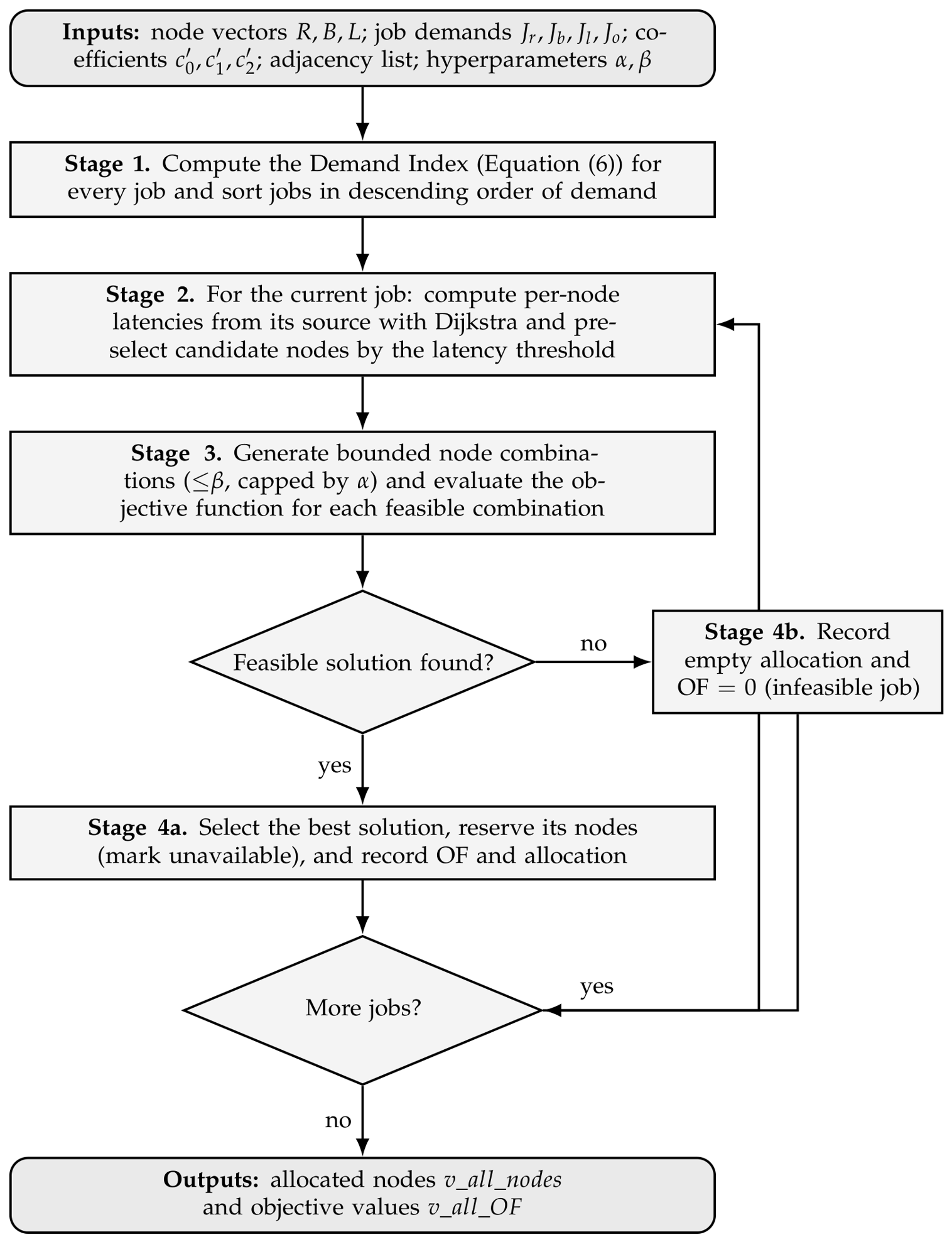
Figure 2 traces the method end to end and illustrates clearly the steps of Algorithm 1. Declaring inputs and outputs at both the figure and the algorithm level, together with the public code repository, is intended to make the workflow fully reproducible.

Regarding the computational complexity of the DI-MNA heuristic, one may observe that the worst-case complexity is dominated by the combinatorial exploration of node subsets for each job. For each job, the algorithm first executes Dijkstra’s shortest-path algorithm, which requires $O\left(ElogV\right)$, $V=\mathrm{nodes},E=\mathrm{edges}$. It then enumerates all subsets of filtered nodes of size up to $\beta$. In the worst case, where all nodes pass the filtering stage, the number of such subsets is ${\sum }_{i=1}^{\beta }\left({\displaystyle \genfrac{}{}{0pt}{}{V}{i}}\right)=O\left(V^{\beta }\right)$. Evaluating each subset requires $O\left(\beta \right)$ time, where $\beta$ is a bounded constant. The overall worst-case time complexity of the heuristic is $O\left(J(ElogV+V^{\beta })\right)$, which is $O\left(J{V}^{\beta }\right)$. The algorithm remains polynomial since $\beta$ is bounded by a small constant.

The hyperparameters $\alpha$$(cut\_comb\_nodes)$ and $\beta$$(cut\_sol)$ introduce bounded combinatorial exploration, thereby rendering the search computationally tractable even in large-scale IoT networks. When $\alpha$ additionally caps the number of candidate combinations evaluated per job, the practical cost becomes $O\left(J·\min (V^{\beta },\alpha )\right)$, i.e., effectively linear in the number of jobs and directly controllable through $\alpha$ and $\beta$. A dedicated calibration study was conducted to assess the influence of these hyperparameters on both solution quality and runtime performance, the results of which are presented and discussed in Section 5.2. The calibration analysis provides empirical support for the simplifying assumption that restricting the maximum number of nodes per job allocation and the number of evaluated node combinations does not, in general, compromise the quality of the obtained solutions while yielding substantial reductions in computational cost.

Termination and convergence. DI-MNA is a constructive single-pass heuristic rather than an iterative search, so it does not rely on stochastic convergence in the sense of a metaheuristic. Termination is guaranteed: the outer loop performs exactly J iterations (one per job, processed in descending Demand Index order), and each inner enumeration is finite and bounded by the hyperparameters $\alpha$ and $\beta$. Because every allocated node is marked unavailable, the candidate set is monotonically reduced and cycling is precluded; the procedure therefore halts in a bounded number of steps for any finite instance.

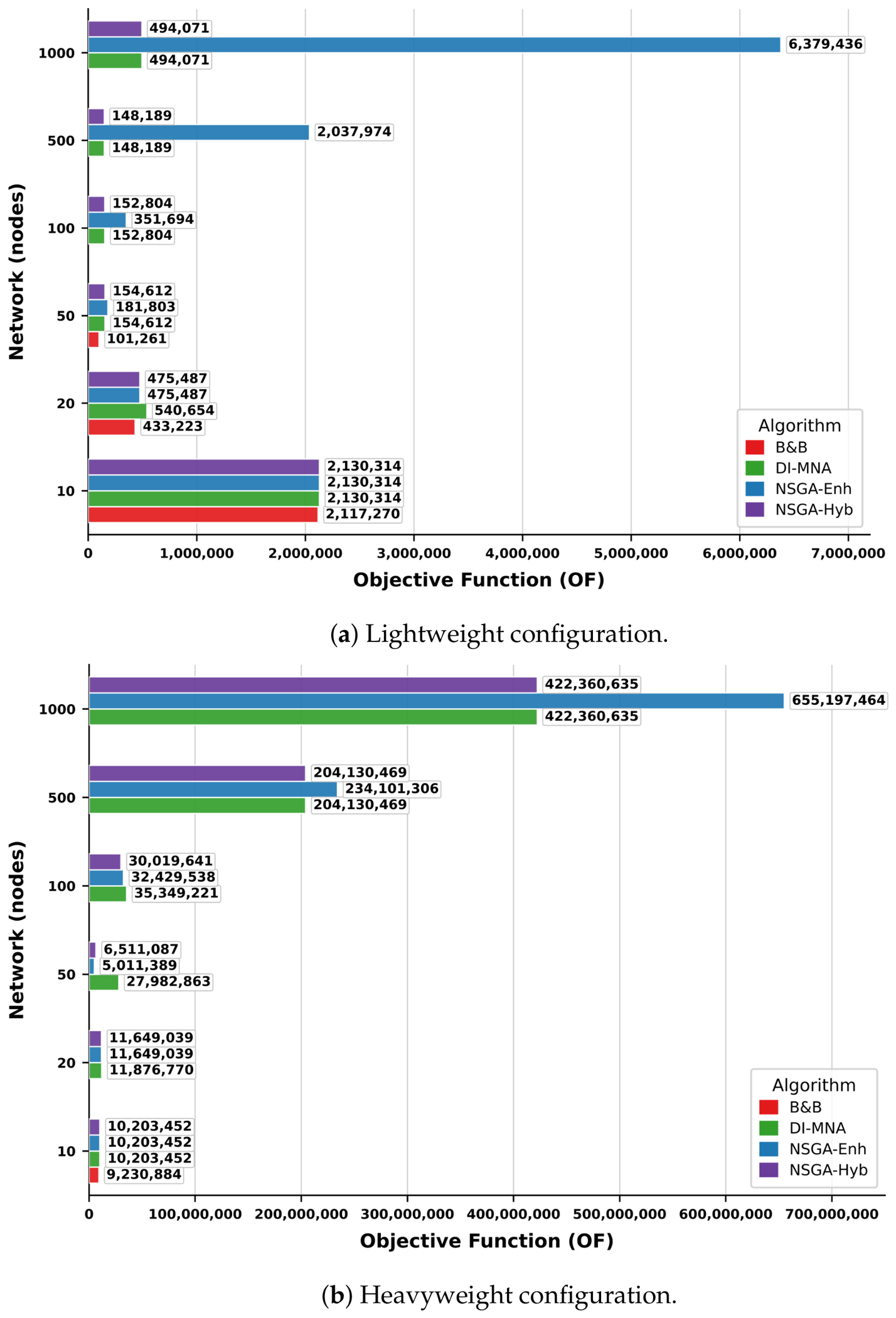
Approximation bounds. As noted in Section 2.1, the MNA problem is structurally analogous to the Generalized Facility Location Problem and is NP-hard. The quadratic surplus terms and the coupled latency constraint render the scalarized objective non-submodular in general, so no constant-factor approximation guarantee can be claimed for the greedy strategy without further restrictive assumptions; we state this limitation explicitly rather than overclaiming. We do not establish a worst-case approximation ratio; instead, we report an empirical optimality-gap analysis against the exact branch-and-bound (B&B) baseline. On 10-node instances, DI-MNA matches the exact optimum whenever B&B is tractable enough to compute it. We leave the derivation of tight approximation bounds for the scalarized MNA objective as an open problem for future work.

4.3. Multi-Node Allocation Based on the NSGA Metaheuristic

The sequential and narrowly focused search of the DI-MNA heuristic often yields suboptimal solutions, especially when strong interdependencies exist among decision variables. The NSGA approach is particularly effective in avoiding solutions stuck in local optima and in discovering non-dominated solutions that form the Pareto front. In algorithms such as NSGA, it is fundamental to model an appropriate encoding of candidate solutions, such as binary or real-valued vectors. Regarding the MNA problem, each individual of a population represents an allocation solution to a job. Each gene of the individuals represents the participation of a specific node in the resource allocation. Additionally, a multidimensional objective function and operational constraints must be established to capture key performance metrics.

In this work, we designed two NSGA-based metaheuristics. The first is denoted as Enhanced NSGA (NSGA-Enh) and operates by adopting the best solution identified across the iterations. In this context, the best solution is defined as the one that attains the lowest objective function (OF) value. The second approach is a hybrid method, referred to as NSGA-Hyb. Its main feature lies in leveraging the best solution from the DI-MNA heuristic as the initial solution to the NSGA’s population. This strategy aims to accelerate convergence and guide the search toward promising regions of the solution space, balancing intensification (local exploration around high-quality solutions) and diversification (exploration of new, previously unexplored regions).

Both metaheuristics share a common evolutionary backbone, whose key components are described as follows. Survivor selection was carried out using the selNSGA3 operator, available in the DEAP (Distributed Evolutionary Algorithms in Python) library [30], configured with 30 reference points uniformly distributed on the normalized reference hyperplane for three objectives, as proposed by [16].

The evolutionary cycle was implemented using the eaMuPlusLambda algorithm, corresponding to the $\mu +\lambda$ strategy, in which the parental population of size $\mu$ and the $\lambda$ offspring generated by the variation operators are evaluated jointly at each generation. This approach introduces implicit elitism into the selection process, ensuring that previously identified feasible solutions are not prematurely discarded.

The combined adoption of selNSGA3 and eaMuPlusLambda is not arbitrary: it establishes an internally consistent evolutionary pipeline in which diversity and elitism are jointly managed by a single unified mechanism, avoiding the methodological inconsistency that would arise from combining crowding distance and reference points within the same selection flow.

Following the guidelines proposed by Deb and Jain [16], the hyperparameter values used in our NSGA-based heuristics are as follows:

• population_size denotes the number of individuals in each generation of the population. In general, values range from 200 to 800 in initial experiments. The value of population_size is increased only in cases of weak convergence or insufficient exploration of the search space. We adopted a $\mathtt{population}\_\mathtt{size}=800$ to ensure adequate exploration of the solution space across all evaluated network sizes.
• generations: The parameter defines the number of generations executed by the algorithm, which typically ranges from 80 to 120. Each generation involves the processes of selection, crossover, and mutation, thereby generating a new population. A total of $\mathtt{generations}=120$ was used in all experiments.
• cx_prob indicates the probability of crossover between two individuals. This value represents the proportion of the population selected to undergo the crossover operation. The typical range of $cx\_prob$ is between $0.7$ and $0.9$ (i.e., $70\%$ to $90\%$) for both continuous and discrete problems. This parameter was set to $\mathtt{cx}\_\mathtt{prob}=0.7$, favoring solution exploitation over excessive diversification.
• indpb: This parameter refers to the mutation probability assigned to each gene, with a typical value defined as $1/total\_nodes$, where each gene represents an IoT network node.When an individual is selected for mutation, this parameter regulates the probability that each gene will be changed within its representation. In this work, $\mathtt{indpb}=0.1$.

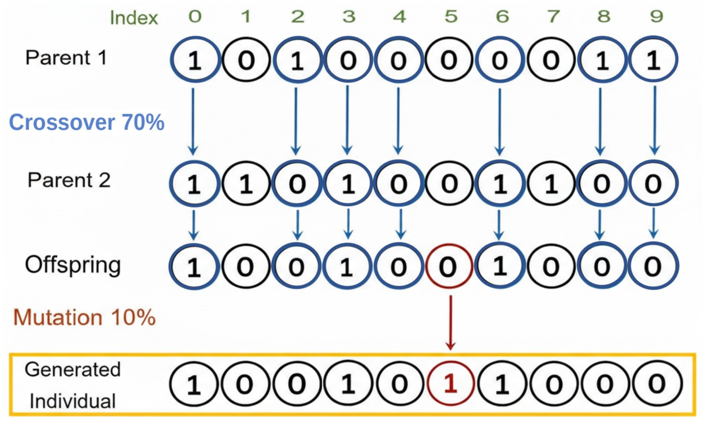
Figure 3 illustrates the crossover and mutation phases performed by the NSGA metaheuristic using 10 genes (representing 10 nodes of an IoT network) for each individual. Uniform crossover is applied at a rate of $\mathtt{cx}\_\mathtt{prob}=0.7$, which implies that, on average, $70\%$ of the selected individual pairs undergo the crossover operation, whereas the remaining $30\%$ are transmitted to the subsequent generation without modification. For each selected pair, the uniform operator determines, at each position of the binary vector, the probability of the gene inheritance from either progenitor. This stochastic process is applied across all genes of the individual, yielding an offspring whose structure combines contributions from both progenitors with equal probability per position, while simultaneously preserving the validity of the binary representation. With a mutation rate of $10\%$, each gene has a $10\%$ chance of being flipped, exemplified here by the bit with index 5 (from left to right). Mutation is essential to prevent premature convergence to suboptimal local solutions and enables the algorithm to explore unvisited regions of the search space. In each generation, individuals are evaluated based on multiple criteria (e.g., latency, resource consumption, and bandwidth), enabling the algorithm to explore the search space under a scalarized objective, producing a set of non-dominated solutions that represent the best tradeoffs between objectives.

This detailed mapping enables the precise application of genetic operators while preserving the characteristics of the MNA problem. It also allows for the incorporation of IoT-specific constraints and features, such as node capacities, job compatibility, and inter-node latencies.

5. Experiments and Results

This section presents the set of experiments and results to evaluate and compare the DI-MNA heuristic and the metaheuristics, NSGA-Enh and NSGA-Hyb.

5.1. Experimental Setup

All simulations were conducted on a workstation equipped with an AMD Ryzen 5 5600G processor (six physical cores, 12 threads, 4.67 GHz clock frequency) and 125 GiB of RAM, running the Linux Debian 6.1.76-1 operating system. The DI-MNA heuristic and the metaheuristics (NSGA-Enh and NSGA-Hyb) were implemented in Python v. 3.12.x, adopting optimized libraries for graph manipulation and numerical analysis. To further support independent validation, all source code, benchmark instances, hyperparameter-tuning outcomes, and configuration files are openly available at https://github.com/lscad-facom-ufms/MNA (accessed on 1 June 2026), so that the community can apply DI-MNA to their own workloads.

The experimental setup was designed to reflect the heterogeneity of large-scale IoT environments, with network sizes ranging from 10 to 1000 nodes. Adhering to the single-layer edge architecture defined in Section 4.1, each network topology was generated as a connected weighted graph in which every communication link was assigned a one-way latency. A shortest-path tree (SPT), rooted at a reference node and computed using Dijkstra’s algorithm, was then derived to represent the primary low-latency communication backbone of the topology, ensuring that every node was connected to the root through its minimum-latency path. Additional edges were subsequently incorporated to increase connectivity, provide routing flexibility, and enable multiple alternative communication paths within the graph. For each network size, nodes were assigned stochastic processing, memory, and bandwidth capacities, while jobs were generated with corresponding requirements for CPU, bandwidth, and latency.

Two input configurations, lightweight and heavyweight, were adopted to assess the heuristics’ performance under different levels of network demands. The configurations were set regarding the number of nodes ($N_{nodes}$) of an IoT network and the number of jobs ($N_{jobs}$): $\rho ={\displaystyle \frac{N_{jobs}}{N_{nodes}}}$. The lightweight configuration assumed a $\rho =20\%$ job-to-node ratio, while the heavyweight targeted a $\rho =70\%$ ratio, representing a near-saturation state. The setup of the light configurations for small-scale network instances (up to 50 nodes) was also evaluated in an optimal B&B algorithm. Each configuration was run $10\times$, from which the mean objective function (OF) and mean runtimes were obtained.

This simulation-based experiment characterizes scalability from 10 up to $100,000$ nodes and benchmarks the heuristics against an exact (B&B) algorithm. Establishing such a ground truth and systematically evaluating both network size and workload (the lightweight and heavyweight configurations) is only feasible in a reproducible simulation, since real testbeds at the ${10}^4$–${10}^5$-node scale are not readily available; simulation therefore enables the optimum-referenced comparison that is central to our evaluation. The generated instances were nonetheless not arbitrary: node and job attributes were drawn from ranges grounded in the edge/IoT literature. In particular, the job latency deadlines spanned 30–250 ms, reflecting real-time and latency-sensitive applications [31], and the one-way link latencies spanned 2–100 ms, reflecting the low-latency infrastructure typical of IoT deployments [32]. Moreover, each topology’s low-latency backbone was a Dijkstra shortest-path tree, augmented with redundant edges to emulate the fault-tolerant mesh connectivity of realistic large-scale IoT networks.

5.2. DI-MNA Hyperparameter Calibration

This section presents the experiment on the hyperparameters $cut\_sol$ and $cut\_comb\_nodes$ of the DI-MNA heuristic. The goal was to find the hyperparameter values that minimized the objective function values and runtime. The hyperparameter calibration experiment was designed by evaluating $cut\_sol=\{2,3\}$ and $cut\_comb\_nodes=\{500,1000,5000\}$.

The hyperparameters analysis showed that the impact of $cut\_sol$ on runtime was more pronounced than $cut\_comb\_nodes$. In large-scale networks (500 to 1000 nodes), the transition from $cut\_sol=2$ to $cut\_sol=3$ had a runtime increase of up to two orders of magnitude. In the lightweight configuration with 1000 nodes, the runtime increased from $7.27\times {10}^{-2}$ s to 2.28 s; in the heavyweight configuration, the increase was from $2.42\times {10}^{-1}$ s to 5.57 s, a high runtime increase compared to an OF improvement (decrease) of less than 0.4%. This behavior was attributed to the combinatorial growth of the search space associated with permitting the allocation of up to three nodes ($cut\_sol=3$) per job.

The experiment also revealed that $cut\_comb\_nodes$ had a small impact on the OF value as the network-size increased. In the lightweight configuration with 1000 nodes, $cut\_sol=2$ and $cut\_comb\_nodes$ values from 500 to 1000, there was an OF decrease from 494,071 down to 266,485, an OF improvement (percentage decrease) of approximately 46%, and a runtime increase from $7.27\times {10}^{-2}$ s to $1.37\times {10}^{-1}$ s. More notably, in the heavyweight configuration, increasing $cut\_comb\_nodes$ did not yield better OF values. These observations indicate that expanding the design space exploration of combinations by increasing $cut\_comb\_nodes$ does not always improve the quality of the solutions.

The non-monotonic behavior observed in the OF value in a 100-node network under the lightweight configuration is particularly noteworthy. Setting $cut\_sol=2$ (regardless of the value of $cut\_comb\_nodes$) yielded OF = 152,804, whereas when $cut\_sol=3$, the OF increased to 226,881. The change from $cut\_sol=2$ to $cut\_sol=3$ did not necessarily lead to an improvement in the OF. This same behavior was also observed in the heavyweight configuration.

The results of the hyperparameter calibration experiment showed that the setup $cut\_sol=2$ and $cut\_comb\_nodes=500$ demonstrated a better balance between the objective function (OF) and runtime, particularly in large IoT networks. The experiment also revealed that limiting the allocation to two nodes per job significantly improved runtime performance without negatively affecting the quality of the objective function in both lightweight and heavyweight scenarios.

5.3. Algorithms Setup and Workload Characteristics

This section presents the algorithms’ setups and the workloads applied to the experiments regarding the DI-MNA heuristic, NSGA-enh, and NSGA-hyb.

Table 4. Hyperparameters of each algorithm.

Algorithm	Hyperparameters
DI-MNA	$cut\_sol=2$, $cut\_comb\_nodes=500$
NSGA-Enh and	$population\_size=800$, $generations=120$,
NSGA-Hyb	$cx\_prob=0.7$, $indpb=1/\text{total\_nodes}$

presents the hyperparameters adopted by each algorithm.

The DI-MNA hyperparameters, $cut\_sol=2$ and $cut\_comb\_nodes=500$, set the maximum number of network nodes assigned to each job and the maximum number of nodes evaluated during each job assignment, respectively. The NSGA-Enh and NSGA-Hyb metaheuristics utilized a $population\_size$ of 800 individuals over 120 generations. The crossover probability was $cx\_prob=0.7$, while the individual mutation probability was set to $indpb=1/total\_nodes$ ($total\_nodes$ corresponds to the total number of nodes in the instance), meaning that the mutation rate adapted to the problem size.

Table 5. Input instances.

Nodes	Instance (Jobs)
	Lightweight	Heavyweight
10	3	7
20	6	14
50	10	35
100	20	70
500	100	350
1000	200	700

characterizes the input instances of the experiments. Each instance is described as the number of nodes of the network and the number of jobs according to the configuration (lightweight or heavyweight).

Table 6. Values of node and job attributes.

Parameter	Unit	Range
Capacity Resource (R)	Units	20–700
Capacity Bandwidth (B)	Mbps	20–5000
Demand Resource ($j_r$)	Units	10–350
Bandwidth Demand ($j_b$)	Mbps	10–2500
Demand Latency ($j_l$)	ms	30–250
Link Latency ($L_{\mathrm{link}}$)	ms	2–100

shows the values of R, B, and L attributes adopted for the network nodes. The atributes required by the set of jobs are also presented.

The input instances were parameterized to enforce the Minimum Node Allocation principle. Specifically, the maximum job resource requirement (${\mathrm{j}}_r=350$) corresponded to half of the maximum processing capacity available at a node ($R=700$). The job’s input parameters were designed to ensure that the job did not demand more resource capacity than the maximum resource capacity of any network node. However, once the node capacities and job demands were assigned randomly, there may have existed a job resource capacity or bandwidth requirement that could not be met by only one network node. Latency considerations were modeled along two complementary dimensions:

• The job latency requirement (${\mathrm{j}}_l$) spanned the interval 30–250 ms, imposing stringent deadlines characteristic of real-time and latency-sensitive applications [31].
• The network link latencies ($L_{\mathrm{link}}$) ranged from 2 to 100 ms, reflecting the low-latency communication properties typically associated with IoT network infrastructures [32].

5.4. Results and Discussion

The experiments were conducted under the lightweight (

Table 7. Results for the lightweight configuration ($\rho =20\%$): mean objective-function value (OF), mean runtime (s), and runtime standard deviation (SD) over ten independent runs. B&B is reported only for the small instances where it remains tractable.

Nodes	Algorithm	OF	Runtime (s)	SD
10	B&B	2,117,270	$3.73\times {10}^{-3}$	$4.00\times {10}^{-5}$
	DI-MNA	2,130,314	$3.68\times {10}^{-3}$	$4.90\times {10}^{-4}$
	NSGA-Enh	2,130,314	$2.21\times {10}^1$	$3.70\times {10}^{-2}$
	NSGA-Hyb	2,130,314	$2.19\times {10}^1$	$7.73\times {10}^{-2}$
20	B&B	433,223	$1.50\times {10}^1$	$1.05\times {10}^{-1}$
	DI-MNA	540,654	$9.23\times {10}^{-3}$	$7.30\times {10}^{-4}$
	NSGA-Enh	475,487	$4.51\times {10}^1$	$5.62\times {10}^{-1}$
	NSGA-Hyb	475,487	$4.42\times {10}^1$	$1.46\times {10}^{-1}$
50	B&B	101,261	$3.18\times {10}^5$	N/A (n = 1)
	DI-MNA	154,612	$4.03\times {10}^{-2}$	$6.20\times {10}^{-4}$
	NSGA-Enh	181,803	$7.68\times {10}^1$	$3.21\times {10}^{-2}$
	NSGA-Hyb	154,612	$7.89\times {10}^1$	$7.38\times {10}^{-2}$
100	DI-MNA	152,804	$2.88\times {10}^{-1}$	$1.51\times {10}^{-3}$
	NSGA-Enh	351,694	$1.80\times {10}^2$	$8.34\times {10}^{-1}$
	NSGA-Hyb	152,804	$1.79\times {10}^2$	$1.25\times {10}^{-1}$
500	DI-MNA	148,189	$6.01\times {10}^1$	$7.79\times {10}^{-1}$
	NSGA-Enh	2,037,974	$1.72\times {10}^3$	$6.07\times {10}^0$
	NSGA-Hyb	148,189	$1.73\times {10}^3$	$1.41\times {10}^0$
1000	DI-MNA	494,071	$1.55\times {10}^2$	$1.49\times {10}^0$
	NSGA-Enh	6,379,436	$5.47\times {10}^3$	$4.83\times {10}^1$
	NSGA-Hyb	494,071	$5.53\times {10}^3$	$2.90\times {10}^1$

) and heavyweight (

Table 8. Results for the heavyweight configuration ($\rho =70\%$): mean objective-function value (OF), mean runtime (s), and runtime standard deviation (SD) over ten independent runs. B&B is reported only for the small instances where it remains tractable.

Nodes	Algorithm	OF	Runtime (s)	SD
10	B&B	9,230,884	$4.63\times {10}^{-2}$	$1.90\times {10}^{-4}$
	DI-MNA	12,117,553	$9.01\times {10}^{-3}$	$1.30\times {10}^{-4}$
	NSGA-Enh	10,203,452	$4.90\times {10}^1$	$2.52\times {10}^{-1}$
	NSGA-Hyb	10,203,452	$5.14\times {10}^1$	$1.44\times {10}^{-1}$
20	DI-MNA	35,505,900	$2.02\times {10}^{-2}$	$5.13\times {10}^{-4}$
	NSGA-Enh	11,649,039	$9.95\times {10}^1$	$6.51\times {10}^{-1}$
	NSGA-Hyb	11,649,039	$9.86\times {10}^1$	$2.03\times {10}^{-1}$
50	DI-MNA	27,982,863	$8.28\times {10}^{-2}$	$6.40\times {10}^{-4}$
	NSGA-Enh	5,011,389	$2.79\times {10}^2$	$2.94\times {10}^{-1}$
	NSGA-Hyb	6,511,087	$2.65\times {10}^2$	$6.69\times {10}^{-1}$
100	DI-MNA	35,349,221	$5.10\times {10}^{-1}$	$1.71\times {10}^{-2}$
	NSGA-Enh	32,429,538	$6.08\times {10}^2$	$7.26\times {10}^0$
	NSGA-Hyb	30,019,641	$6.34\times {10}^2$	$3.45\times {10}^0$
500	DI-MNA	204,130,469	$9.02\times {10}^1$	$2.13\times {10}^0$
	NSGA-Enh	234,101,306	$9.89\times {10}^3$	$5.19\times {10}^1$
	NSGA-Hyb	204,130,469	$5.98\times {10}^3$	$3.44\times {10}^1$
1000	DI-MNA	422,360,635	$3.78\times {10}^2$	$3.20\times {10}^0$
	NSGA-Enh	655,197,464	$3.15\times {10}^4$	$8.47\times {10}^1$
	NSGA-Hyb	422,360,635	$1.93\times {10}^4$	$3.32\times {10}^1$

) configurations. Four algorithmic approaches were evaluated: the exact B&B method, the proposed DI-MNA heuristic, and the metaheuristics NSGA-Enh and NSGA-Hyb. Each pair (input instance and algorithm) was run ten times (the only exception is the B&B algorithm with 50 nodes), and the results were evaluated on the objective function (OF) value, mean runtime, and runtime standard deviation.

5.4.1. Solution Quality

One way to evaluate and compare the algorithms is based on the objective function (OF) values across the set of input instances. The results presented in Table 7 and Table 8, and illustrated in Figure 4a,b, provide a detailed understanding of the solution quality (OF values) of the exact B&B algorithm in comparison to the DI-MNA, NSGA-Enh, and NSGA-Hyb.

Regarding the lightweight configuration, the three heuristic approaches demonstrate high precision in small-scale instances of 10 nodes, converging to an OF of 2,130,314. This value represents a percentage difference of less than 1% from the B&B algorithm. As the network size increases, the OF values of DI-MNA and NSGA-Hyb maintain constant parity, reaching identical values for networks with 50, 100, 500, and 1000 nodes. NSGA-Enh exhibits progressive degradation, notably for the 1000-node scenario, where the OF is approximately 13 times higher than DI-MNA.

In the context of heavyweight configurations, a different behavior is observed at intermediate network sizes. In the 50-node network, the NSGA approaches outperform the DI-MNA. The percentage change between the OF solution from NSGA-Enh and DI-MNA achieves 82%. This suggests that the evolutionary operators are initially more effective at handling dense and complex search spaces. However, upon reaching the 1000-node network, it suffers from premature convergence to local optima, resulting in an objective function value of 655,197,464. In contrast, DI-MNA converges alongside NSGA-Hyb to a value of 422,360,635. The percentage change between DI-MNA and NSGA-Enh shows an OF value decrease of $35\%$.

The comparative synthesis on the OF values indicates that the DI-MNA heuristic achieves the best results upon large-size IoT networks. In the 500 and 1000-node scenarios for both light and heavy configurations, DI-MNA attained the best solution quality among the heuristics. Figure 4 shows that, in the lightweight configuration, DI-MNA and NSGA-Hyb converge to identical OF from 50 nodes onward, while NSGA-Enh degrades progressively (up to ≈13× worse at 1000 nodes); in the heavyweight setting, the evolutionary variants attain better OF across the small-to-intermediate range (10–100 nodes). At 500–1000 nodes, the DI-MNA and NSGA-Hyb converge to the same value. The practical consequence is that seeding and running additional NSGA generations does not improve on DI-MNA at scale. NSGA-Hyb is initialized with the DI-MNA solution and never surpasses it on the large instances; the extra evolutionary budget yields no solution-quality benefit while incurring the runtime penalties (Section 5.4.2).

Table 9. Percentage change (PC) of the OF relative to the exact B&B optimum (baseline) for the lightweight configuration at 10, 20, and 50 nodes; lower values indicate closer agreement with the optimum.

Algorithm	Percentage Change
	10 nds	20 nds	50 nds
DI-MNA	0.62%	24.80%	52.69%
NSGA-Hyb	0.62%	9.76%	52.69%
NSGA-Enh	0.62%	9.76%	79.54%

presents the percentage change (PC—Equation (8)) regarding the OF values of algorithms DI-MNA, NSGA-Hyb, and NSGA-Enh compared to the B&B (baseline). The percentage was calculated for the lightweight networks of 10, 20, and 50 nodes, and it was used to evaluate the quality of the heuristics’ results (OF).

$$\mathrm{PC}={\displaystyle \frac{O{F}_{\mathrm{Baseline}}-O{F}_{\mathrm{Algorithm}}}{O{F}_{\mathrm{Baseline}}}}$$

(8)

where $O{F}_{\mathrm{baseline}}$ is the objective function values achieved by the $B\&B$ algorithm and $O{F}_{\mathrm{algorithm}}$ denotes the OF values from the DI-MNA, NSGA-Hyb, and NSGA-Enh.

For small instances (10 nodes), all algorithms exhibited the same difference. In intermediate networks (20 nodes), NSGA-Enh stood out with the lowest deviation from the baseline. In larger networks (50 nodes), the DI-MNA and NSGA-Hyb achieved the best results. The same results from DI-MNA and NSGA-Hyb show that the NSGA approach does not improve the results of the greedy heuristic.

One can observe that the results of DI-MNA and NSGA-Hyb are quite similar for larger networks (100, 500, and 1000 nodes in Figure 4). Setting NSGA-Enh as a baseline and comparing its results in the 1000-node network, the percentage change to DI-MNA (and NSGA-Hyb) is up to $92.2\%$ and $35.5\%$ in the lightweight and heavyweight configurations, respectively.

Table 10. Objective-function (OF) descriptive statistics over the ten runs of each lightweight instance for DI-MNA and NSGA-Hyb, with the Wilcoxon signed-rank outcome ($\alpha =0.05$).

Nodes	DI-MNA OF	NSGA-Hyb OF	CV a	Wilcoxon Outcome
10	2,130,314	2,130,314	$0.00\%$	Tie—no difference
20	540,654	475,487	$6.76\%$	NSGA-Hyb lower, 5/10 ($p=0.0625$)
50	154,612	154,612	$0.00\%$	Tie—no difference
100	152,804	152,804	$0.00\%$	Tie—no difference
500	148,189	148,189	$0.00\%$	Tie—no difference
1000	494,071	494,071	$0.00\%$	Tie—no difference

^a The OF column reports the best (minimum) value attained over the ten runs, and the CV column reports the coefficient of variation of the NSGA-Hyb. DI-MNA is a deterministic single-pass heuristic, so its OF is the same across the ten runs ($\mathrm{CV}\equiv 0\%$, median equal to the reported value, IQR $=0$, and a $95\%$ CI that collapses to the point value). NSGA-Hyb likewise converged to a single OF at every instance except the 20-node one, where it reached a lower OF in five of the ten runs (tied with DI-MNA in the remaining five); on that instance the paired Wilcoxon signed-rank test yielded $p=0.0625$, so the difference was not significant at $\alpha =0.05$.

shows the differences in objective function (OF) values between DI-MNA and NSGA-Hyb were assessed with the non-parametric Wilcoxon signed-rank test on the paired per-run results at a significance level of $\alpha =0.05$; the Wilcoxon test was preferred over the paired t-test because normality could not be assumed for such small samples. On larger networks (100, 500, and 1000 nodes in the lightweight configuration, and 500/1000 nodes in the heavyweight configuration), DI-MNA and NSGA-Hyb attained identical OF values, so the paired differences were zero, and the test indicated that the additional NSGA generations did not improve upon DI-MNA. The same held at 10 and 50 nodes in the lightweight configuration. The only exception was the 20-node lightweight instance, where NSGA-Hyb had a lower OF but the difference was not statistically significant at $\alpha =0.05$ (Wilcoxon signed-rank test, $p=0.0625$).

Positioning against recent state-of-the-art approaches. Beyond the exact B&B, DI-MNA was benchmarked against NSGA-III, one of the most widely adopted reference-point-based many-objective evolutionary algorithms, a standalone metaheuristic (NSGA-Enh) and a hybrid seeded with the heuristic output (NSGA-Hyb). Relative to the recent methods surveyed in Section 3 ([18,19,20,22,24,26,28]), DI-MNA differs into two aspects: (i) it explicitly supports Multi-Node Allocation over general (cyclic) graph topologies rather than trees or single-node assignment, and (ii) it sustains polynomial, low-variance runtime at the ${10}^3$–${10}^5$-node scale.

Table 11. Statistical significance of the objective-function (OF) comparison between DI-MNA and NSGA-Hyb (lightweight configuration), using the Wilcoxon signed-rank test ($\alpha =0.05$).

Nodes	DI-MNA vs. NSGA-Hyb	Test	Outcome
10	Identical (2,130,314)	Wilcoxon	Tie—no difference
20	Difference (5/10 runs)	Wilcoxon	NSGA-Hyb lower ($p=0.0625$)
50	Identical (154,612)	Wilcoxon	Tie—no difference
100	Identical (152,804)	Wilcoxon	Tie—no difference
500	Identical (148,189)	Wilcoxon	Tie—no difference
1000	Identical (494,071)	Wilcoxon	Tie—no difference

summarizes these outcomes for the lightweight configuration.

5.4.2. Computational Performance

The analysis of the runtime demonstrated a better performance of the DI-MNA heuristic over the assessed algorithms. Figure 5a,b illustrate the algorithms’ runtimes across the input instances and configurations.

Figure 5a,b shows that DI-MNA outperforms all other algorithm approaches. The speedup performance metric (Equation (9)) was applied to quantify the runtime performance gains.

$$\mathrm{Speedup}=\left({\displaystyle \frac{T_{\mathrm{Algorithm}}}{T_{\mathrm{Baseline}}}}\right)$$

(9)

where $T_{\mathrm{baseline}}$ and $T_{\mathrm{algorithm}}$ denote the average execution times of the baseline and the tested algorithm, respectively.

Regarding the lightweight configurations in 10-node instances, DI-MNA has a runtime of $3.68\times {10}^{-3}$ s, while the NSGA-Enh and NSGA-Hyb require approximately 22 s, resulting in a speedup exceeding 5900. This superior performance is sustained in large-scale scenarios (1000 nodes), where DI-MNA requires only $1.55\times {10}^2$ s, remaining approximately 35 times faster than the evolutionary metaheuristics.

The runtime behavior of DI-MNA is even better under heavyweight configurations, where the structural density of the problem is heightened. At an input instance of 1000 nodes, DI-MNA runtime is $3.78\times {10}^2$ s, while NSGA-Enh and NSGA-Hyb require $3.15\times {10}^4$ s and $1.93\times {10}^4$ s, respectively. Notably, the transition between low- and high-density instances increases the runtime of DI-MNA by only 2.4 times, demonstrating significantly lower sensitivity to instance complexity compared to NSGA-based approaches.

The runtime differences compared to the B&B algorithm underscores the practical usage of the $B\&B$ approach as problem dimensionality increases. In 50-node networks under lightweight configuration, B&B reached the threshold of intractability, demanding $3.18\times {10}^5$ s for a single run. In contrast, DI-MNA using the same instance achieved $4.03\times {10}^{-2}$ s, representing a speedup of over $7.8\times {10}^6$ times. In summary, DI-MNA seems to find allocation solutions within practical runtime for large-scale IoT networks.

Table 12. Runtime speedup of DI-MNA, NSGA-Hyb, and NSGA-Enh relative to the exact B&B baseline (lightweight configuration) at 10, 20, and 50 nodes.

Algorithm	Speedup
	10 nds	20 nds	50 nds
DI-MNA	1.01407	1626.81523	7,891,748.172
NSGA-Hyb	0.00017	0.33975	4030.83146
NSGA-Enh	0.00017	0.33316	4145.26633

presents the speedup of DI-MNA, NSGA-Hyb, and NSGA-Enh over $B\&B$. Figure 5 (log scale) shows that the gaps of one to three orders of magnitude translate into a concrete operational difference: at 1000 nodes DI-MNA produces an allocation in minutes ($1.55\times {10}^2$ s lightweight, $3.78\times {10}^2$ s heavyweight), whereas the evolutionary metaheuristics require several hours (∼$5.5\times {10}^3$–$3.15\times {10}^4$ s). This runtime budget makes DI-MNA feasible for large-scale, time-constrained IoT scheduling, where an allocation decision cannot wait hours to be produced.

The runtime gaps were large and consistent across instances. The Wilcoxon signed-rank test on the paired runtime samples confirmed that DI-MNA was significantly faster than both NSGA variants ($p<0.05$) at every network size, and the reported speedups (e.g., $35\times$ and $51\times$ over NSGA-Hyb at 1000 nodes for the lightweight and heavyweight configurations) were outside the 95% confidence intervals of the compared means.

Reporting the runtime SD is motivated by the predictability of the response time. A scheduler that is fast on average but highly variable is unsuitable for latency-sensitive, real-time deployments, so the SD complements the mean by quantifying the run-to-run dispersion, and this is exactly where DI-MNA stands out (Figure 6).

Table 13. Runtime descriptive statistics over the ten runs of each lightweight instance: median, interquartile range (IQR), $95\%$ confidence interval (CI) of the mean, and coefficient of variation (CV), for DI-MNA and NSGA-Hyb.

Nodes	Algorithm	Median (s)	IQR (s)	95% CI (s)/CV
10	DI-MNA	$3.51\times {10}^{-3}$	$5.00\times {10}^{-5}$	$[3.33,4.03]\times {10}^{-3}$/$13.2\%$
	NSGA-Hyb	$2.19\times {10}^1$	$4.52\times {10}^{-2}$	$[21.84,21.96]$/$0.35\%$
20	DI-MNA	$8.96\times {10}^{-3}$	$2.70\times {10}^{-4}$	$[8.71,9.75]\times {10}^{-3}$/$7.9\%$
	NSGA-Hyb	$4.42\times {10}^1$	$3.91\times {10}^{-2}$	$[44.10,44.30]$/$0.33\%$
50	DI-MNA	$4.03\times {10}^{-2}$	$6.05\times {10}^{-4}$	$[3.99,4.07]\times {10}^{-2}$/$1.53\%$
	NSGA-Hyb	$7.90\times {10}^1$	$8.06\times {10}^{-2}$	$[78.85,78.95]$/$0.09\%$
100	DI-MNA	$2.88\times {10}^{-1}$	$2.26\times {10}^{-3}$	$[2.869,2.891]\times {10}^{-1}$/$0.53\%$
	NSGA-Hyb	$1.79\times {10}^2$	$1.15\times {10}^{-1}$	$[178.91,179.09]$/$0.07\%$
500	DI-MNA	$6.02\times {10}^1$	$1.08\times {10}^0$	$[59.54,60.66]$/$1.30\%$
	NSGA-Hyb	$1.73\times {10}^3$	$1.31\times {10}^0$	$[1.729,1.731]\times {10}^3$/$0.08\%$
1000	DI-MNA	$1.55\times {10}^2$	$1.95\times {10}^0$	$[153.9,156.1]$/$0.96\%$
	NSGA-Hyb	$5.55\times {10}^3$	$4.27\times {10}^1$	$[5.51,5.55]\times {10}^3$/$0.52\%$

The $95\%$ CI was computed as $\mathrm{mean}\pm t_{0.025,9}\mathrm{SD}$/$\sqrt{10}$ from the ten runs. The larger CV of DI-MNA at 10–20 nodes reflects its sub-second runtimes (a small denominator), not larger absolute variability: its absolute SD and CI remain orders of magnitude tighter than those of NSGA-Hyb at every scale.

reports the coefficient of variation ($\mathrm{CV}=\mathrm{SD}/\mathrm{mean}$) alongside the median, IQR, and $95\%$ CI, so that dispersion is also expressed on a scale-independent basis. The CV should be considered carefully for DI-MNA, whose sub-second runtimes at small scales inflate the relative dispersion even though the absolute SD and CI remain orders of magnitude tighter than those of the metaheuristics; the absolute predictability, which is what matters for real-time scheduling, therefore favors DI-MNA across all scales.

The runtime stability of the DI-MNA heuristic can be observed in the values of the SD column in Table 7 and Table 8. For small-scale instances (10 and 20 nodes), DI-MNA exhibits low standard deviations, ranging from $4.90\times {10}^{-4}$ to $7.30\times {10}^{-4}$. As network size increases (50, 100, 500, and 1000 nodes), DI-MNA sustained a low runtime variance compared to that of the metaheuristics. Figure 6 presents the standard deviation of each algorithm on the lightweight and heavyweight configurations and the set of network sizes.

DI-MNA maintains the lowest runtime standard deviations (SDs) across all evaluated network scales, consistently remaining at orders of magnitude below the other algorithms. Regarding the genetic algorithms, it is observed that their instability behavior (SD) is similar, with both being orders of magnitude more unstable than DI-MNA.

In small-scale instances, such as 10, 20, and 50-node networks, DI-MNA has very close runtime standard deviations independent of the configuration. These results highlight that the runtime stability of the heuristic is minimally impacted by workload density. As the input instance increases, the visual profile in Figure 6 reveals that DI-MNA preserves a linear and controlled runtime stability, whereas the NSGA algorithms exhibit sharp divergences and more pronounced instability peaks under high demand (heavyweight) networks.

DI-MNA is a deterministic, single-pass constructive heuristic whose per-instance work is bounded by its hyperparameters, so its runtime dispersion stays low and grows smoothly with network size. The NSGA variants, in contrast, are population-based stochastic searches whose per-run cost depends on the convergence dynamics of the evolutionary loop; under heavy workload, this stochasticity produces the sharp instability peaks seen in Figure 6. The two genetic variants exhibit similar instability to each other, both orders of magnitude above DI-MNA. This predictability is what qualifies DI-MNA for real-time IoT scheduling, a point taken up in the Discussion (Section 6).

The data corroborate the existence of a performance hierarchy among the approaches. The B&B algorithm, while guaranteeing optimal solutions, lacks scalability. NSGA-Enh is sensitive to instance size. In contrast, NSGA-Hyb demonstrates greater resilience in preserving solution quality; however, its application entails a computational burden one to three orders of magnitude higher than that observed for the DI-MNA algorithm, which stands out for its runtime performance.

Scalability beyond 1000 nodes. To assess applicability to very large deployments, DI-MNA was evaluated on networks of 10,000 and 100,000 nodes under both lightweight ($\rho =20\%$) and heavyweight ($\rho =70\%$) configurations. Both network sizes adopted the same hyperparameters values ($cut\_comb\_nodes=500$ and $cut\_sol=2$). The heuristic allocated all jobs successfully, confirming that the bounded combinatorial exploration kept the method tractable at these scales, consistent with the $O\left(J{V}^{\beta }\right)$ worst-case complexity established in Section 4.2.

5.5. Boundary Conditions and Failure Modes

This subsection draws on the discipline of formal heuristic analysis to state the guarantees that hold, the regimes in which they do not, and a conditional theoretical boundary on the incurred loss.

Guarantees that hold. Within the bounded search defined by the hyperparameters $cut\_comb\_nodes$ and $cut\_sol$, DI-MNA is exhaustive per job: it evaluates every feasible node combination among the pre-filtered candidates and selects the objective minimizer. Consequently, for any job that is satisfiable by at most $cut\_sol$ nodes within the pruned candidate set, DI-MNA returns the optimal single-job allocation.

Exceptional cases. We identify three regimes in which the greedy, sequential strategy can be exceeded:

• Sequential myopia. Because jobs are allocated one at a time in descending Demand Index order and allocated nodes become unavailable to later jobs, an early high-demand allocation may consume a node that would have been globally preferable for a subsequent job. This coupling is the source of the medium-scale heavyweight cases (e.g., 50 and 100 nodes) in which the NSGA metaheuristics located slightly better objectives.
• The β bound. If a job requires strictly more than $\beta$ nodes to be met, the bounded search cannot represent that allocation. In our instances ($J_r\le 350$ against node capacity $R\le 700$), jobs were typically satisfiable within $\beta =2$; the bound can nonetheless be raised at a controlled polynomial cost of $O\left(V^{\beta }\right)$ when denser demands are anticipated.
• The α pruning. Capping the number of evaluated combinations can, on adversarial instances, exclude a globally optimal combination. The calibration study (Section 5.2) empirically bounded this effect and supported $\alpha =500$, $\beta =2$ as a robust operating point across both lightweight and heavyweight configurations.

Conditional theoretical boundary. For a single job, let ${\mathrm{OPT}}_{\beta }$ denote the optimal objective value achievable using at most $\beta$ nodes from the full candidate set. DI-MNA returns exactly ${\mathrm{OPT}}_{\beta }$ whenever the $\alpha$ pruning does not discard the optimizing combination. The only loss relative to the unrestricted optimum is therefore bounded by two terms: (a) the gap between ${\mathrm{OPT}}_{\beta }$ and the true optimum for jobs that genuinely require more than $\beta$ nodes, and (b) the sequential (no-sharing) coupling across jobs. Both terms vanish under the stated modeling assumptions, which explains the near-optimality observed empirically. Consistent with the non-submodular nature of the scalarized objective (Section 4.2), we present this as a conditional guarantee rather than a distribution-free, constant-factor approximation ratio, whose existence for the coupled quadratic-plus-latency objective remains an open problem.

6. Discussion

This section synthesizes the experimental findings, interprets their significance, and positions DI-MNA relative to the exact, evolutionary, and multi-node approaches evaluated in this study.

Synthesis of the findings. Three consistent patterns emerge across the experiments. In terms of solution quality (Section 5.4.1, Figure 4, Table 9 and Table 10), DI-MNA reaches the exact B&B optimum whenever B&B remains tractable (a $0.62\%$ percentage change at 10 nodes) and matches NSGA-Hyb on every large instance, the Wilcoxon test returning a formal tie. In terms of computational performance (Section 5.4.2, Figure 5, Table 12), DI-MNA is one to three orders of magnitude faster than the metaheuristics and up to $7.8\times {10}^6$ times faster than B&B, producing 1000-node allocations in minutes rather than hours. In terms of stability (Figure 6, Table 13), its absolute runtime dispersion stays orders of magnitude below the evolutionary variants at every scale.

Significance. Taken together, these results show that DI-MNA delivers near-optimal solution quality at a polynomial, predictable runtime, and that this combination is what enables the method to scale to ${10}^4$–${10}^5$ nodes (

Table 14. Extended-scale behavior of DI-MNA on networks of 10,000 and 100,000 nodes under light and heavy configurations. All runs used the calibrated pruning hyperparameters ($\alpha =500$ and $\beta =2$).

Nodes	Configuration	Jobs	Pruning ($\mathit{\alpha }$, $\mathit{\beta }$)	All Jobs Allocated
10,000	Lightweight ($\rho =20\%$)	2000	$\alpha =500$, $\beta =2$	Yes
10,000	Heavyweight ($\rho =70\%$)	7000	$\alpha =500$, $\beta =2$	Yes
100,000	Lightweight ($\rho =20\%$)	20,000	$\alpha =500$, $\beta =2$	Yes
100,000	Heavyweight ($\rho =70\%$)	70,000	$\alpha =500$, $\beta =2$	Yes

) where both the exact baseline and the metaheuristics are impractical. The equivalence with NSGA-Hyb on large instances is particularly informative: because NSGA-Hyb is seeded with the DI-MNA solution and never improves upon it at scale, the additional evolutionary budget buys no solution-quality gain, only a cost. Predictable, low-variance runtime is itself a first-class property for latency-sensitive IoT scheduling, not a secondary concern.

Comparison with existing approaches. Against the exact B&B method, DI-MNA trades a negligible optimality gap for tractability, since B&B is already intractable beyond 50 nodes. Against NSGA-Enh, DI-MNA is markedly more robust: the standalone metaheuristic is sensitive to instance size and degrades sharply on large lightweight networks (up to ≈13× worse OF at 1000 nodes). Against NSGA-Hyb, DI-MNA is quality-equivalent but one to three orders of magnitude faster. Relative to the closest prior work explicitly targeting Multi-Node Allocation [28], DI-MNA differs by supporting general cyclic topologies, by providing an exact-optimization benchmark, and by demonstrating scalability well beyond the scales reported there.

Balanced interpretation. The evidence is not uniformly one-sided. In specific medium-scale, heavy-load niches (e.g., 50 nodes, heavyweight), the evolutionary operators still locate marginally better optima than DI-MNA, because at intermediate density the stochastic exploration can escape the local structure that the greedy construction commits to early. This advantage, however, is confined to a narrow scale band and comes at the cost of the temporal predictability and scalability that dominate the large-scale regime, which is the regime this work targets.

SDN-based QoS control. SDN decouples the control plane from the data plane, giving a centralized controller a global topology view that it uses for QoS-aware routing, bandwidth reservation, and traffic engineering on behalf of latency-sensitive, interactive applications [33,34]. DI-MNA operates at a complementary layer: it decides which node subsets should jointly serve each job under processing, bandwidth, and latency constraints. An SDN control plane is therefore a natural substrate to enforce DI-MNA’s decisions: the heuristic supplies the Multi-Node Allocation, and the controller installs the corresponding low-latency routes and bandwidth guarantees that preserve the high-level QoS metrics (end-to-end delay, jitter, throughput) of real-time interactive workloads [35]. This positions DI-MNA as an allocation-decision component that is orthogonal to, and integrable with, SDN-QoS mechanisms rather than competing with them.

Real-time frameworks and resource management systems. DI-MNA embodies the discipline of real-time resource management systems (rtf-rms): a class of frameworks that allocate compute, memory, and network resources to online, interactive applications subject to explicit timing guarantees, performing admission control and placement so that end-to-end deadlines are consistently met [36]. Modern containerized rtf-rms for edge/fog/cloud IoT, such as the FogBus2 framework and its lightweight container-orchestration extensions, were designed precisely to schedule and place latency-critical IoT workloads across distributed, heterogeneous nodes while keeping deployment and management overhead low [37,38]. DI-MNA maps directly onto this discipline. In DI-MNA, the feasibility constraint (5) ($F_L\left(i\right)\ge 0$) enforces that the end-to-end communication delay of an allocation does not exceed the application’s tolerated latency, thereby acting as an admission-control and placement criterion: a candidate node subset is admitted only when its aggregated processing and bandwidth capacities, together with its Dijkstra-computed least-latency communication path, jointly satisfy the resource, bandwidth, and deadline requirements of the job. Complementarily, the latency-margin term $F_L\left(i\right)$ of the scalarized objective (1) actively maximizes the remaining temporal slack, supplying exactly the headroom that real-time managers rely on to absorb runtime variability, jitter, and transient load fluctuations without breaching deadlines. The job-deadline range adopted in our experiments (30–250 ms) is characteristic of real-time and interactive IoT workloads [31,36], so the feasibility test and the slack-maximizing objective together reproduce, at the allocation layer, the two operations (deadline-constrained admission and slack-aware placement) that define an rtf-rms.

Within this framing, DI-MNA can be embedded within an rtf-rms as its Multi-Node Allocation strategy, in contrast to frameworks that assume single-node placement or that manage timing without exploiting resource aggregation across cooperating nodes [37,38]: when no individual node can meet a job’s demand on its own, DI-MNA composes a feasible subset whose joint capacity does, while still honoring the end-to-end latency deadline. Crucially, an rtf-rms is judged not only by the quality of the placements it produces but also by the cost and, above all, the predictability of the scheduling decision itself, since the manager’s own decision latency is part of the end-to-end response budget of interactive applications [15,19]. DI-MNA’s low and predictable decision latency (Figure 6, Table 13)—a direct consequence of its deterministic, single-pass construction bounded by the hyperparameters $\alpha$ and $\beta$—is therefore a first-class property for real-time managers, and it distinguishes DI-MNA from the population-based metaheuristics whose run-to-run variability would propagate into the timing behavior of the host framework. This positions DI-MNA as a deadline-aware, resource-aggregating allocation component that composes naturally with existing real-time resource management frameworks for interactive cloud/IoT applications [36,37,38], rather than competing with them.

7. Conclusions and Future Work

This work presented new heuristics for the MNA problem in small and large-scale IoT networks. The algorithmic approaches were capable of finding feasible solutions even under highly demanding scenarios. Specifically, the Demand Index heuristic approach (DI-MNA) balanced resource usage and latency and adopted a preselection mechanism that ensured manageable runtimes.

Regarding the runtime on large-scale networks, the DI-MNA outperformed both NSGA metaheuristics. The speedup of the DI-MNA over the NSGA-Hyb was $35\times$ and $51\times$ on networks with 1000 nodes, using light and heavy configurations, respectively. When comparing the objective function results in large-scale networks with lightweight and heavyweight configurations, DI-MNA attained similar results to NSGA-Hyb, showing that, even after running additional NSGA generations, the metaheuristic did not improve the results of DI-MNA.

The results also revealed that the scenarios and network size may impact the quality and performance of the proposed MNA methods. In specific medium-scale and high-load scenarios (e.g., 50 nodes, heavyweight), the metaheuristic approaches may identify slightly better objective function (OF) values. This result indicates that stochastic exploration may find more favorable local minima in moderate complexity networks. Additionally, for very small instances ($N\le 20$), the B&B exact method remained the benchmark for optimal solutions, although it became computationally infeasible beyond 50 nodes. The DI-MNA heuristic was also evaluated on IoT networks with $10,000$ and $100,000$ nodes under both light and heavy configurations. All jobs were successfully allocated, demonstrating the robustness and scalability of the proposed DI heuristic.

Although the study presents promising results, some limitations can be identified. First, the network model adopted simplifying assumptions to enable the application of heuristic techniques, such as considering an IoT architecture composed of a single layer (edge layer), assuming that all nodes remained active throughout the allocation process, and adopting a specific communication topology. Such premises may limit the generalization of the results to hierarchical edge–fog–cloud IoT network architectures or environments with dynamically unavailable nodes. Furthermore, although the experiments were conducted on networks with up to 1000 nodes, the validation was performed exclusively in a simulated environment, without evaluation under real-world conditions.

Future research directions on this work are as follows:

• New experiments on the automatic adjustment of parameters and weights to cope with scenarios where the assigned network resources (nodes and edges) can be shared among jobs.
• Designing parallel MNA algorithms. The inner loop of DI-MNA enumerates and evaluates candidate node combinations independently for each job, which is a potential candidate for parallelism; other strategies, inspired by the parallelization of exact and metaheuristic solvers in the classical optimization literature, include partitioning the job stream and the node-combination enumeration across workers and evaluating candidate combinations in parallel (master–worker and island-model schemes).
• A further direction is the deployment of DI-MNA within a software-defined networking (SDN) control plane, which would let the heuristic supply Multi-Node Allocation decisions while the controller installs the corresponding low-latency routes and bandwidth reservations to preserve end-to-end QoS for real-time interactive applications.
• Another research possibility is to adopt new resource constraints, such as incorporating an explicit energy-consumption term into the objective function, which the current utilization-minimizing formulation only approximates indirectly.
• Extending the comparison to other metaheuristic approaches (e.g., MOPSO and WOA adapted to the single-layer, latency-constrained MNA model) is also planned to further strengthen the benchmarking.
• Evaluating DI-MNA on real-world datasets and measured traces across different network scales and deploying it on a physical edge/IoT testbed. This will allow us to assess robustness under measured latency variability, node churn (dynamically unavailable nodes), and heterogeneous device profiles.