Resource-Efficient Continual Learning for Medicinal Plant Identification: A Periodic Retraining Approach for Edge-Deployed Agricultural IoT Applications

Abstract

Smartphone-based plant identification increasingly serves as the edge tier of agricultural Internet of Things (IoT) systems, where models must adapt to crowdsourced data under bandwidth, memory, and energy constraints. No prior work, to our knowledge, has systematically investigated continual learning at the scale of thousands of fine-grained medicinal plant species from crowdsourced images, nor how retraining frequency affects the cost–performance trade-off in an IoT model-lifecycle setting. We evaluate three continual learning strategies, naïve fine-tuning, experience replay, and Learning without Forgetting, under periodic retraining schedules (updating every K increments), tested on 2719 species (≥25 images each) from the Viet Medi Species 2026 dataset (310,647 images; 4799 species total). All three strategies exhibit negative forgetting (performance improvement rather than degradation) in the instance-incremental setting, with naïve fine-tuning and LwF showing the strongest gains. Periodic retraining with $K=2$ halves retraining operations while maintaining comparable performance. A baseline MobileNetV2 model achieves 54.07% top-10 accuracy across 2719 species and has been deployed via TensorFlow Lite (FP16, ∼11.5 MB) in the Med Herb Lens Android application. In this regime, naïve fine-tuning offers a favourable cost–performance trade-off and is a reasonable default for instance-incremental agricultural IoT deployments.

1. Introduction

Recent studies show that deep learning algorithms can correctly identify plant species about 90% of the time [1]; thus far, there are proven applications of deep learning to support species identification in practical agricultural and ecological settings, namely, mobile plant identification systems like Pl@ntNet [2] and smartphone-assisted diagnosis of crop disease [3]. However, accuracy rates vary significantly between datasets and across application scenarios, highlighting the need to evaluate deep learning performance in specific contexts.

One application where accuracy is particularly critical is the identification of medicinal plants. Accurate identification is essential for protecting medicinal plant species, documenting traditional medicines, and providing data for the development of new pharmaceuticals.

The diversity of medicinal plants in Vietnam offers a unique opportunity to apply deep learning-based species identification. Nguyen Quoc and Truong Hoang [4] found that deep learning architectures can achieve very good results on the identification of Vietnamese medicinal plants with an accuracy of 88.26% for Xception using the VNPlant-200 dataset [5] consisting of 20,000 images over 200 species of plants. More recent application of Vision Transformers to VNPlant-200 has achieved over 99% accuracy on this dataset [6], demonstrating that contemporary deep learning architectures can achieve expert-like accuracy in the classification of botanic specimens from Vietnam. However, it is important to note that these high accuracies were achieved on a comparatively small classification problem (200 species); classification difficulty increases substantially as the number of visually similar species grows, and top-1 accuracy alone becomes a less informative metric at larger scales. In such contexts, ranked candidate lists and top-k accuracy, where classification is considered correct if the correct species appears among the first k candidates, better reflect practical identification workflows.

Previous research identified a number of challenges in implementing deep learning models in field deployment settings, including rapidly changing environmental conditions, limited connectivity in rural areas, and restrictions in energy and computational capabilities, necessitating adaptive modelling alternatives rather than static solutions [7]. Since training data increments continuously via crowdsourced submissions rather than as a complete dataset, trained models must be able to continue gaining knowledge without losing any previously acquired knowledge.

Such smartphone-driven, crowdsourced species identification is increasingly understood as a form of agricultural and ecological IoT sensing rather than a standalone mobile-app problem. GPS-enabled smartphones running on-device classifiers act as edge nodes in distributed sensing networks, capturing image, location, and timestamp metadata and feeding it back to centralised systems for aggregation, model retraining, and over-the-air (OTA) redistribution [8,9]. Framing identification systems this way makes explicit the constraints that govern their lifecycle—bandwidth, on-device memory, intermittent connectivity, and energy—and motivates a model-update strategy that respects those constraints. The remainder of this paper accordingly treats Med Herb Lens not as a single mobile app but as the edge tier of an agricultural IoT pipeline whose update cadence is set by the periodic retraining strategy under investigation. We note upfront that the cloud retraining trigger is currently invoked manually rather than by an automated event-driven trigger; the edge and gateway tiers are operationally deployed (Section 6.3.3), and the empirical parameters identified in this study are intended to inform the operational settings of the automated trigger when it is deployed.

The challenges of deploying deep learning models in field settings require models that can adapt continuously. Continual learning—the ability to learn continuously—has thus emerged as an active research area for addressing these deployment challenges [10]. However, a major challenge in continual learning is catastrophic forgetting, as identified by McCloskey and Cohen [11], where a neural network rapidly forgets previously learned information when learning from new data. Thus, this has driven research into the different forms of integrating new knowledge (more plasticity) with previously learned knowledge (more stability; i.e., memory) [12].

The most recent comprehensive surveys illustrate that there are three primary ways to mitigate catastrophic forgetting: (1) regularisation-based methods (restricting how weight updates occur); (2) replay-based methods (methods to keep examples of previous data); and (3) architecture-based methods (whereby parts of a model are given to different tasks) [13,14]. Van de Ven and Tolias [15] propose a framework for categorising continual learning, identifying three scenarios: task-incremental, domain-incremental and class-incremental. This framework was subsequently established as foundational to continual learning research [16].

Despite much progress made within the field, continual learning has not yet been fully developed for the application of large-scale fine-grained botanical classification. The majority of continual learning studies have considered learning from benchmark datasets that contain between tens and hundreds of classes [13], whereas many plant identification application systems must identify thousands of visually similar plant species. Moreover, most contemporary work in continual learning is focused on class-incremental scenarios, where the number of classes changes over time, rather than instance-incremental scenarios, where the number of instances changes—a pattern that more closely resembles crowdsourced plant observation data collection.

Given these three broad categories and the instance-incremental setting of our study, we selected three continual learning strategies that span the spectrum of forgetting mitigation. The first, naïve fine-tuning, applies no explicit forgetting mitigation and serves as a lower-bound baseline—the model is simply updated on each new data increment using standard backpropagation. The second, experience replay, is a replay-based approach that maintains a memory buffer of randomly sampled examples from prior increments and interleaves them with new data during training [17]. The third, Learning without Forgetting (LwF), is a regularisation-based method that uses knowledge distillation from a frozen copy of the previous model to preserve learned representations without requiring access to stored exemplars [18]. Architecture-based methods were excluded from this comparison because they are designed primarily for task-incremental settings where new output heads are added over time, and they scale poorly to thousands of classes in an instance-incremental scenario where the class set remains fixed [19,20]. This selection thus allows a direct comparison between no mitigation, data-centric mitigation, and model-centric mitigation under identical periodic retraining conditions.

From a practical perspective, designers of agricultural IoT pipelines for plant identification must make key choices about how often models are retrained and redistributed, and how compute, memory, and bandwidth are budgeted across edge, gateway, and cloud tiers. Online learning approaches that update models continuously demand a constant supply of compute and connectivity. A periodic batch retraining approach—updating the model at fixed intervals (e.g., every two weeks)—offers more predictable resource usage and a cleaner mapping onto OTA update cycles, while still allowing new knowledge to enter the model promptly. The appropriate balance is determined by application requirements, the rate at which observations arrive, the connectivity profile of deployed edge devices, and the available cloud compute budget—none of which have been systematically studied for fine-grained plant identification at scale.

Motivated by the gaps above, this paper investigates one main research question:

RQ: 

How can continual learning be deployed efficiently and reliably as the model-update component of an agricultural IoT pipeline for large-scale fine-grained medicinal plant identification?

We address this through three specific sub-questions:

RQ1: 

Among continual learning strategies that span the spectrum of forgetting mitigation—naïve fine-tuning, experience replay, and Learning without Forgetting—which is most effective for instance-incremental learning at the scale of thousands of fine-grained species?

RQ2: 

How does the periodic retraining frequency (parameterised by the retraining period K) affect the trade-off between model quality and the operational costs of an IoT update pipeline (cloud compute, OTA bandwidth, per-device update energy)?

RQ3: 

What end-to-end edge–gateway–cloud architecture connects on-device inference, crowdsourced observation upload, periodic retraining, and OTA model distribution into a coherent model lifecycle under intermittent connectivity, and what practical guidelines—covering strategy selection, retraining frequency, memory budgeting, and connectivity-aware OTA scheduling—follow for adaptive learning systems in agricultural IoT settings?

Table 1. Comparison of this work with representative prior studies on medicinal plant classification. Key differentiators of our study are highlighted: large-scale species count, continual learning with periodic retraining, and edge IoT deployment. The bold row denotes the present work.

Study	Species	Images	Learning Paradigm	Architecture	Deployment
Nguyen Quoc & Truong Hoang [4]	200	20 K	Static (single-round)	Xception	None
Nhut et al. [6]	200	20 K	Static (single-round)	ViT/BEiT	None
Nguyen & Ngo [21]	109	28 K+	Static (single-round)	MobileNetV2	None
Dat et al. [22]	29	373	Static (single-round)	EfficientNet + MobileNet	None
Zhang et al. [23]	300	52 K+	Static (single-round)	Multiple CNNs	None
This work	2719	310 K+	Instance-incremental with periodic retraining	MobileNetV2	Med Herb Lens (Android, edge IoT)

summarises how this work differs from prior studies in medicinal plant classification. While existing studies focus on static, single-round training with small to moderate species counts, our work introduces a periodic retraining framework for continual learning at a scale not previously examined in the medicinal plant literature, coupled with practical deployment as the edge tier of an agricultural IoT pipeline.

Specifically, we make the following contributions:

• A periodic retraining strategy for resource-efficient continual learning (Algorithm 1): A scheduled update strategy where models retrain every K increments rather than after each data addition, quantifying the trade-off between computational savings and model performance.
• A systematic investigation of catastrophic forgetting in large-scale instance-incremental learning: We evaluate naïve fine-tuning, experience replay, and Learning without Forgetting on 2719 fine-grained species—a scale and learning scenario not previously examined in the medicinal plant classification literature.
• To our knowledge, the largest continual learning study of Vietnamese medicinal plants: In total, 2719 species, substantially exceeding the scale of previous studies (typically 100–300 species), with cross-seed consistency checks.
• Actionable deployment recommendations for edge-deployed agricultural IoT pipelines: Concrete guidelines on strategy selection, retraining frequency, memory budgeting, and connectivity-aware OTA scheduling, informed by the Med Herb Lens Android application currently deployed on Google Play.
• An end-to-end agricultural IoT model-lifecycle architecture: A three-tier edge–gateway–cloud pipeline (Section 6.3) that connects on-device TensorFlow Lite inference, crowdsourced observation upload, periodic retraining, and OTA model distribution, mapping the periodic retraining frequency K directly onto operational bandwidth and energy costs.

Algorithm 1 Periodic Batch Retraining Strategy

Require:  Data increments $\{D_1,D_2,\dots ,D_R\}$, retraining period K, model $\theta$  1:  Train $\theta$ on base data ${\mathcal{D}}_0$  2:  Record base evaluation accuracy $a_0$  3:  for $r=1$ to R do  4:     if $r\mathrm{mod}K=0$ then  5:          Train $\theta$ on increment ${\mathcal{D}}_r$ using selected strategy  6:          Evaluate $\theta$ on held-out base evaluation set  7:          Record accuracy $a_r$ and compute forgetting $F_r=a_0-a_r$  8:     else  9:          Skip increment ${\mathcal{D}}_r$ (no model update; data discarded; $a_r=a_{r-1}$) 10:     end if 11:  end for 12:  return Forgetting curve $\{F_1,F_2,\dots ,F_R\}$

The remainder of this paper addresses the main RQ above as follows. Section 2 reviews related work on continual learning, plant classification, and edge AI/IoT for ecological sensing. Section 3 describes the dataset, the instance-incremental learning setup, the continual learning strategies evaluated, and the evaluation metrics. Section 4 details the experimental setup and implementation. Section 5 presents and analyses the empirical findings, addressing RQ1 and RQ2. Section 6 interprets the results, presents the IoT system architecture and OTA model lifecycle (addressing RQ3), discusses limitations, and outlines future work. Section 7 concludes. Together, these sections establish both the empirical basis and the practical deployment guidance for resource-efficient continual learning in agricultural IoT settings.

2. Related Work

2.1. Continual Learning Paradigms

Continual (incremental) learning refers to approaches that allow a machine learning model to learn new information from incoming sequential datasets while maintaining access to previously learned information [10]. Continual learning aims to solve the problem of catastrophic forgetting, which occurs when the model is trained with new datasets and catastrophically loses performance on previous datasets [11,12].

Van de Ven and Tolias [15] proposed a framework that divides three types of problems into different categories based on the task structure and inferences made during learning. In task-incremental learning, task identity is provided at test time, allowing task-specific output heads. In domain-incremental learning, the same classes appear across tasks but with distribution shifts. In class-incremental learning, new classes are introduced over time, and the model must distinguish among all classes without task identity information. This taxonomy was formalised in subsequent work demonstrating that scenario selection fundamentally affects method effectiveness [16].

The scenario most relevant to crowdsourced plant identification is instance-incremental learning, where new training examples arrive for existing classes rather than introducing new categories. Read et al. [24] provided early analysis distinguishing batch-incremental from instance-incremental processing for data streams, though this setting has received less attention in deep learning research compared to class-incremental scenarios.

Recent comprehensive surveys have systematically organised the continual learning literature. De Lange et al. [13] conducted an extensive experimental comparison of 11 methods and 4 baselines across multiple datasets, which introduced the stability-plasticity trade-off framework. Masana et al. [14] evaluated 13 class-incremental methods investigating domain shift effects. Wang et al. [25] provided theoretical foundations alongside method categorisation, while Zhou et al. [26] offered a detailed analysis of approaches that are data-centric, model-centric, and algorithm-centric. These surveys consistently group catastrophic-forgetting mitigation strategies into three families—regularisation-based, replay-based, and architecture-based—which we summarise in turn below.

Regularisation-based methods limit weight modifications to preserve knowledge important to previous data. Kirkpatrick et al. [27] introduced Elastic Weight Consolidation (EWC), which uses the Fisher information matrix to identify and protect important parameters; Zenke et al. [28] proposed Synaptic Intelligence (SI), which estimates parameter importance online during training. Li and Hoiem [18,29] introduced Learning without Forgetting (LwF), which uses knowledge distillation from a frozen teacher network to preserve previous behaviour without requiring access to prior training data.

Replay-based methods maintain a memory of examples from previous training phases and interleave them with new data. Shin et al. [30] proposed deep generative replay using GANs to synthesise samples from previous task distributions. Rebuffi et al. [31] introduced iCaRL, combining nearest-mean-of-exemplars classification with herding-based exemplar selection and knowledge distillation; notably, the iCaRL paper explicitly states that “finetuning always achieves the worst results” in class-incremental scenarios—a finding that contrasts with our instance-incremental results. Lopez-Paz and Ranzato [32] proposed Gradient Episodic Memory (GEM) and introduced formal metrics for forward and backward transfer evaluation, while van de Ven et al. [33] demonstrated that brain-inspired generative replay effectively prevents catastrophic forgetting across all three scenarios.

Architecture-based methods allocate distinct model components to different tasks; representative examples include Progressive Neural Networks [19] and PackNet [20]. As discussed in Section 1, these methods are designed primarily for task-incremental settings and scale poorly to thousands of fixed classes, so they are not considered further in this study.

2.2. Plant Classification with Deep Learning

Deep learning methods and advancements have enabled an incredible evolution in plant classification; comprehensive literature reviews have described this rapid evolution [1]. A systematic review of literature was conducted by Mulugeta et al. [1], which included 31 studies from 2018 through 2022, applying PRISMA guidelines. In the review, the authors found that 96.8% of studies classified plants based on leaf organs, 83.8% of studies used transfer learning, and 64.5% of studies used CNNs as their primary classification algorithm.

Mohanty et al. [3] completed baseline studies to compare AlexNet and GoogLeNet with transfer learning from the ImageNet dataset and demonstrated >99% accuracy using the PlantVillage dataset (54,306 total images) containing images of 38 different plant species, thereby demonstrating the effective use of transfer learning for plant disease classification and identification of plant species.

Picek et al. [34] benchmarked current state-of-the-art methods for CNNs and Vision Transformers using PlantCLEF datasets; for example, ViT-Large achieved an accuracy of 91.15% on PlantCLEF 2017, and the authors reported that retrieval-based classification approaches outperformed classification approaches by 0.28–10.25%.

Specifically regarding Vietnamese medicinal plants, Nguyen Quoc and Truong Hoang [4] completed a comparative study of several architectures (VGG16, ResNet-50, InceptionV3, DenseNet-121, Xception, MobileNet) and reported that Xception achieved the highest accuracy on VNPlant-200 (88.26%). Their VNPlant-200 companion dataset paper [5] is the first publicly available large-scale dataset for Vietnamese medicinal plants with 20,000 images of 200 species.

Additional work on Vietnamese plant classification includes Nguyen and Ngo [21], who achieved 83.9% accuracy with MobileNetV2 on 109 Vietnamese species, and Dat et al. [22], who proposed a multimodel CNN combining EfficientNet and MobileNet with joint multiloss functions for Vietnamese herb identification.

2.3. Edge AI and IoT for Ecological Sensing

Edge AI—the practice of running inference directly on resource-constrained sensing devices rather than sending data to the cloud—has emerged as a central paradigm for ecological and agricultural monitoring under field conditions. Vuilliomenet et al. [9] reviewed 82 studies published between 2017 and 2025 and identified four broad system types for biodiversity monitoring: (1) TinyML on low-power microcontrollers for single-taxon detection, (2) single-board-computer-class edge devices for multi-species classification, (3) distributed edge AI, and (4) cloud AI used for retrospective processing. The smartphone-based deployment investigated in this paper sits in the second of these tiers—edge devices with sufficient compute for multi-species classification but constrained relative to cloud GPUs. Earlier surveys of agricultural deep learning [7] similarly identified unreliable connectivity, limited power, and the need for real-time processing as the dominant practical constraints, motivating model architectures designed for on-device inference.

Lightweight architectures targeting field deployment have been a particularly active area. Guan et al. [35] proposed Dise-Efficient, achieving 99.80% accuracy on PlantVillage with a 13.3 MB model. Zhou et al. [36] developed REM-ShuffleNetV2 (4.40M parameters, 96.72% accuracy on a field crop disease task). Our use of MobileNetV2 with FP16 TensorFlow Lite quantisation (∼11.5 MB) sits within this same lightweight-edge regime.

Closer to the present work, Lourenço et al. [37] surveyed on-device edge learning for IoT data streams, explicitly connecting continual learning to the constraints of TinyML and IoT edge deployments. They emphasise that data architecture (batch versus stream) and network capacity (cloud versus edge) jointly determine which continual learning algorithms are feasible—an observation that directly motivates our investigation of periodic retraining as a middle ground between continuous online updates and infrequent full retraining. The optimal balance between online learning and batch retraining depends on application requirements, data arrival rates, and available computational budget, and these considerations are precisely what an IoT model-lifecycle framing makes tractable.

2.4. Summary of Research Gaps

The literature reviewed above reveals several key gaps that this work addresses. First, while deep learning has been extensively applied to plant classification, existing studies on medicinal plants are limited to small-scale datasets (typically 80–300 species) and employ static, single-round training without consideration of how models should be updated as new data arrives. Second, the continual learning literature has focused predominantly on class-incremental scenarios using benchmark datasets with tens to hundreds of classes, leaving instance-incremental learning at the scale of thousands of fine-grained species largely unexplored. Third, to our knowledge, no prior work has systematically evaluated the trade-off between retraining frequency and computational cost for plant identification systems, despite this being a critical deployment consideration for resource-constrained edge IoT deployments. Finally, while several Vietnamese medicinal plant datasets exist, none have been coupled with a continual learning evaluation pipeline and a deployed edge-tier IoT application. This study addresses all four gaps through a large-scale empirical investigation of periodic retraining strategies on 2719 Vietnamese medicinal species, yielding both novel findings (negative forgetting in instance-incremental learning) and practical IoT deployment guidance.

3. Methodology

This section describes our empirical approach to examining periodic retraining methodologies for large-scale classification of Vietnamese medicinal plants. We will discuss our dataset, define the instance-incremental learning environment, explain the continual learning methodologies assessed, and describe our evaluation methods.

3.1. Dataset Description

The dataset we used in this research was the Viet Medi Species 2026 [38], a large-scale multilingual image dataset tailored for medicinal plants documented in Vietnamese traditional medicine. The dataset comprises 310,647 images from 4799 accepted species spanning four kingdoms (Plantae, Fungi, Chromista, and Bacteria), integrated with the Global Biodiversity Information Facility (GBIF) taxonomic backbone. To the best of our knowledge, this contains one of the largest fine-grained datasets of images of medicinal plants available for research purposes.

Table 2. Comparison of Viet Medi Species 2026 with related plant classification datasets. Values in bold denote the dataset introduced in this work.

Dataset	Species	Images	Viet Names
PlantCLEF 2023 [39]	80,000	4 M	0%
VNPlant-200 [5]	200	20 K	100%
DIMPSAR [40]	80	12.8 K	0%
TCMP-300 [23]	300	52 K+	0%
Viet Medi Species 2026	4799	310 K+	84%

positions the Viet Medi Species 2026 dataset relative to other prominent plant classification datasets, demonstrating its scale advantage.

The dataset was constructed through a systematic five-stage pipeline described in detail by Tran et al. [38]: (i) taxonomic normalisation of species lists from the Vietnamese Medicinal Plant Catalogue (Danh lục cây thuóc Việt Nam) using the GBIF Species Match API; (ii) image acquisition from GBIF’s Occurrence API, capped at 130 images per species to limit class imbalance; (iii) Vietnamese vernacular name curation for 4031 species (84% coverage) through over 320 h of manual research and validation against authoritative sources, with regional naming variations preserved with cultural attribution; (iv) quality control and filtering, retaining only species with at least 25 images for the experiments in this study, yielding 2719 usable classes (≥25 images each); and (v) metadata integration following Darwin Core standards. All curation code is openly available on GitHub (release v1.1), and the complete image archive and metadata are deposited on Kaggle, enabling full reproducibility.

Beyond curation, the dataset offers an extensive increase over currently available Vietnamese plant datasets. The VNPlant-200 dataset [5] contains 20,000 images across 200 species, while our dataset scales to 2719 usable species classes—over 13 times more classes. This scale substantially exceeds prior Vietnamese medicinal plant datasets and is comparable to recent large-scale efforts such as TCMP-300 for Chinese medicinal plants [23], though it remains well below the diversity of PlantCLEF challenges which have addressed up to 80,000 species [39]. Beyond benchmarking deep learning architectures, this scale also serves as a stress test for edge-deployable models: 2719 fine-grained classes pose a substantially harder learning problem than the 100–300-class settings typical of prior medicinal plant work, while the deployed model must still fit within the size, memory, and energy budget of a smartphone-class edge device.

The dataset exhibits attributes characteristic of real-world crowdsourced biodiversity collections:

• Long-tail distribution: Long-tailed distributions of species frequencies; there are many pictures of common species, while there are almost none of rare species near the minimum threshold level.
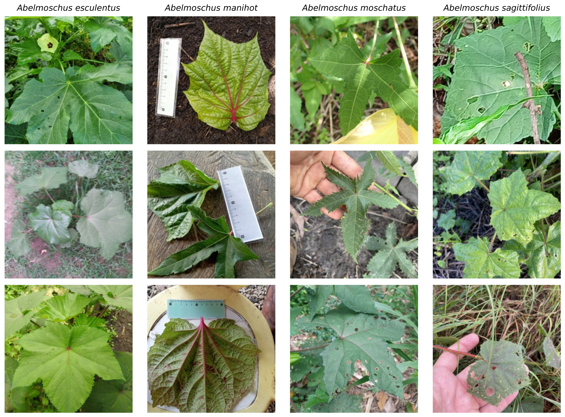
• High visual similarity: High similarity among visual characteristics of many species of the same genus, requiring very fine disambiguation of characteristics for these species (Figure 1).
• Intra-class variation: A wide range of image characteristics of the plants due to the differences in the growing conditions, times of day, and quality of images taken in the field shows the diversity of plant data collected in the field.
• Vietnamese nomenclature: Scientific and Vietnamese common names (vernacular) for each species are displayed to promote cultural appropriateness of ecological and biodiversity applications.

Table 3. Dataset statistics overview for Viet Medi Species 2026.

Attribute	Value
Total accepted species	4799
Usable classes (≥25 images)	2719
Minimum images per class	25
Maximum images per class	130
Image resolution	Variable (resized to 224 × 224)
Learning paradigm	Instance-incremental (IIL)

summarises the dataset characteristics used in our experiments.

3.2. Instance-Incremental Learning Scenario

We formulate the learning problem as instance-incremental learning (IIL), where the class set $\mathcal{C}$ of $C=2719$ classes remains fixed while new training examples arrive over time. This scenario reflects realistic crowdsourced data collection, where users contribute additional images of known species rather than discovering entirely new species.

Following the incremental learning formalisation of van de Ven et al. [16], we define the following notation. Let R denote the total number of increments. Each increment $r\in \{1,2,\dots ,R\}$ provides a new batch of training data ${\mathcal{D}}_r$. We partition each class’s images into:

• Base training set: 20 images per class for initial model training
• Increment sets: Up to 10 images per class per increment, arriving sequentially over up to 9 increments, depending on the number of images available for that class beyond the base and evaluation sets
• Held-out evaluation set: 5 images per class, fixed throughout for measuring forgetting

This partitioning simulates a deployment scenario where an initial model is trained on available data, then periodically updated as new field observations accumulate. The held-out evaluation set enables consistent measurement of catastrophic forgetting across all experimental conditions. Because the dataset filter retains classes with at least 25 images, a class at the minimum threshold contributes its full 20 base and 5 evaluation images but zero increment images; classes with between 26 and 114 images contribute a proportionally truncated sequence of increments (e.g., a class with 50 images supplies the base set, the evaluation set, and approximately 2–3 increments before its image pool is exhausted). The full 9-increment schedule is therefore exercised only by classes with at least 115 images. Long-tail classes are not excluded by this scheme—they continue to contribute to the held-out evaluation set throughout—but they participate in fewer retraining events than head classes, which mirrors the data-availability profile of real crowdsourced collections.

Instead of retraining the model after each increment of data received, we propose periodic retraining, which updates the model once every K increments. At increment r where $\left(r\mathrm{mod}K\right)=0$, the model trains on that increment’s data for a fixed number of epochs. Increments where $\left(r\mathrm{mod}K\right)\ne 0$ are skipped—the model does not update, and the data from these skipped increments is not retained for later use. This strategy reflects practical IoT edge scenarios where devices have limited storage and can only retain the most recent data batch rather than accumulating historical increments. The approach represents a compromise between continuous online learning and infrequent batch retraining. Algorithm 1 presents the procedure.

Using $R=9$ increments and $K=2$, this periodic retraining model will perform a total of 4–5 updates instead of 9, creating approximately 50% less training work. During skipped increments, the model weights remain frozen, resulting in zero forgetting (no performance change) until the next retraining event.

3.3. Continual Learning Strategies

We evaluate three continual learning strategies designed to address the effects of catastrophic forgetting. All strategies were chosen based upon their frequency of appearance in recent surveys [13,14]:

3.3.1. Naïve Fine-Tuning

In this method, the model is trained on new data from each increment using only standard cross-entropy loss functions, without any explicit efforts to mitigate catastrophic forgetting. Let ${\mathcal{D}}_r={\left\{(x_i,y_i)\right\}}_{i=1}^{N_r}$ denote the training set available at increment r, where $x_i$ is an input image, $y_i$ is the corresponding class label, and $N_r$ is the number of samples. Let $\theta$ denote the set of trainable parameters of the model $f_{\theta }$. The cross-entropy loss for a single sample $(x,y)$ is defined as

$${\mathcal{L}}_{\mathrm{CE}}(f_{\theta }\left(x\right),y)=-\log \left({\displaystyle \frac{\exp \left(z_y\right)}{{\sum }_{j=1}^C\exp \left(z_j\right)}}\right)$$

(1)

where $z=f_{\theta }\left(x\right)\in {\mathbb{R}}^C$ is the logit vector output by the model for C classes, and $z_y$ is the logit corresponding to the true class y. The parameters $\theta$ are updated to minimise the average loss over the training set:

$${\mathcal{L}}_{\mathrm{naive}}(\theta ;{\mathcal{D}}_r)={\displaystyle \frac{1}{N_r}}{\displaystyle \sum _{i=1}^{N_r}}{\mathcal{L}}_{\mathrm{CE}}(f_{\theta }\left(x_i\right),y_i)$$

(2)

This baseline is critical for establishing whether sophisticated continual learning methods provide benefits over simple fine-tuning in the instance-incremental scenario.

3.3.2. Experience Replay

Experience replay maintains a memory buffer storing representative examples from previous data, following the approach established in foundational work on replay methods [17]. During training on new increments, samples from the replay buffer are interleaved with current data. We use reservoir sampling to maintain 10 examples per class in the buffer. Let ${\mathcal{D}}_{\mathrm{new}}$ denote the training samples from the current increment and ${\mathcal{D}}_{\mathrm{buffer}}$ denote the samples stored in the replay buffer. The combined training set is ${\mathcal{D}}_{\mathrm{combined}}={\mathcal{D}}_{\mathrm{new}}\cup {\mathcal{D}}_{\mathrm{buffer}}$, and the parameters $\theta$ are updated to minimise

$${\mathcal{L}}_{\mathrm{replay}}(\theta ;{\mathcal{D}}_{\mathrm{combined}})={\displaystyle \frac{1}{|{\mathcal{D}}_{\mathrm{combined}}|}}\sum _{(x,y)\in {\mathcal{D}}_{\mathrm{combined}}}{\mathcal{L}}_{\mathrm{CE}}(f_{\theta }\left(x\right),y)$$

(3)

3.3.3. Learning Without Forgetting (LwF)

LwF employs knowledge distillation [41] to preserve the model’s predictions on new data from before the update, following Li and Hoiem [18]. A frozen copy of the model with parameters ${\theta }_{\mathrm{old}}$ (the teacher) provides soft targets that regularise the updated model with parameters $\theta$ (the student). Let ${\mathcal{D}}_r$ denote the training set at increment r. The combined loss function is

$${\mathcal{L}}_{\mathrm{LwF}}(\theta ;{\mathcal{D}}_r)={\displaystyle \frac{1}{N_r}}{\displaystyle \sum _{i=1}^{N_r}}\left[(1-\alpha ){\mathcal{L}}_{\mathrm{CE}}(f_{\theta }\left(x_i\right),y_i)+\alpha {\mathcal{L}}_{\mathrm{KD}}(\theta ,{\theta }_{\mathrm{old}};x_i)\right]$$

(4)

where $\alpha$ controls the balance between new learning and knowledge retention (set to 0.7 in our experiments). The knowledge distillation loss ${\mathcal{L}}_{\mathrm{KD}}$ is defined using temperature-scaled softmax outputs. Let $z=f_{\theta }\left(x\right)$ and $z_{\mathrm{old}}=f_{{\theta }_{\mathrm{old}}}\left(x\right)$ denote the logit vectors produced by the student and teacher models, respectively. The temperature-scaled softmax function $\sigma$ with temperature T is

$$\sigma {\left({\displaystyle \frac{z}{T}}\right)}_j={\displaystyle \frac{\exp (z_j/T)}{{\sum }_{k=1}^C\exp (z_k/T)}}$$

(5)

where the subscript j denotes the j-th element of the resulting probability vector. The knowledge distillation loss is then the Kullback–Leibler (KL) divergence between the teacher’s and student’s temperature-scaled outputs:

$${\mathcal{L}}_{\mathrm{KD}}(\theta ,{\theta }_{\mathrm{old}};x)=T^2·\mathrm{KL}\left(\sigma \left({\displaystyle \frac{z_{\mathrm{old}}}{T}}\right)\parallel \sigma \left({\displaystyle \frac{z}{T}}\right)\right)$$

(6)

The factor $T^2$ compensates for the reduced magnitude of gradients when using temperature scaling. Temperature T controls the smoothness of the predicted probability distributions: higher values produce softer targets that encode more information about inter-class similarities, while $T=1$ reduces to standard cross-entropy. We set $T=2$ following the recommendation of Hinton et al. [41], which has been shown empirically to balance informative soft targets with training stability across diverse classification tasks. The teacher network is refreshed after each retraining step to serve as the reference for the next update.

3.4. Evaluation Metrics

We employ metrics focused on quantifying catastrophic forgetting in our instance-incremental learning setting. Let $a_r$ denote the top-1 accuracy evaluated on the held-out base evaluation set after training on increment r. We use top-1 accuracy here (rather than the top-10 metric reported for the full-data baseline in Section 5.6) because forgetting is most clearly observed when the model’s single highest-confidence prediction changes; top-1 is also the standard metric in the continual learning literature on which our experimental design is based [16,32]. Specifically, $a_0$ represents the base accuracy after initial training on ${\mathcal{D}}_0$ (the base training set), and $a_r$ for $r>0$ represents the accuracy after retraining on increment ${\mathcal{D}}_r$. Under periodic retraining with period K, $a_r$ is only updated when $r\mathrm{mod}K=0$; at other increments, $a_r=a_{r-1}$ (i.e., the model is not retrained and performance remains unchanged).

Base evaluation accuracy. After each retraining step, we evaluate accuracy on the fixed held-out base evaluation set (5 images per class). This quantifies how well a model retains its ability to perform on the original data distribution after it has been updated.

Forgetting. Forgetting $F_r$ at increment r is defined as the decrease in base evaluation accuracy relative to the initial baseline:

$$F_r=a_0-a_r$$

(7)

where $a_0$ is the base accuracy (after initial training on ${\mathcal{D}}_0$) and $a_r$ is the accuracy at increment r. Positive values of $F_r$ indicate forgetting (i.e., degradation of performance) while negative values indicate improvement. We report both mean forgetting $\overline{F}={\displaystyle \frac{1}{R}}{\sum }_{r=1}^R{F}_r$ (averaged across all increments) and final forgetting $F_R$ (after the last increment R).

Computational efficiency. We measure wall-clock training time to characterise the computational requirements of each strategy. Combined with the periodic retraining framework (parameterised by K), this enables analysis of efficiency–performance trade-offs.

4. Experimental Setup

MobileNetV2 is chosen for continual learning because its compact architecture is well suited to edge deployment in agricultural IoT settings. The model has ImageNet pre-trained weights with the final fully connected layer replaced with a classifier that defines all 2719 species classes.

The images are resized to be 224 × 224 pixels and normalised based on the ImageNet statistics. We apply light data augmentation during training, consisting of random horizontal flips and minor colour jitter to improve generalisation.

Table 4. Training hyperparameters.

Parameter	Value
Backbone architecture	MobileNetV2
Pre-training	ImageNet
Optimiser	Adam
Learning rate	0.0001
Batch size	16
Epochs (base training)	8
Epochs (incremental)	3
Epochs (converged-base control)	up to 40 (early-stopped)
Early stopping patience	2 epochs
Mixed-precision training	enabled (FP16)
Input resolution	224 × 224
IIL-specific parameters
Base images per class	20
Increment images per class	10
Number of increments	9
Evaluation images per class	5
Strategy-specific parameters
Replay buffer per class	10
LwF distillation weight ($\alpha$)	0.7
LwF temperature (T)	2.0
Retraining period (K)	2, 5

summarises the training hyperparameters.

Our experiments evaluate periodic retraining with $K=2$, where the model is retrained every 2nd increment. With 9 total increments, $K=2$ results in 4–5 retraining operations, representing approximately 50% reduction compared to retraining after every increment. The evaluation of each method (naïve, replay and LwF) was done under the same conditions to ensure fair comparison between methods. To validate the reliability of our results, we performed experiments with three random seeds (42, 123 and 456). Experiments were conducted on NVIDIA P100 GPU hardware through Kaggle’s computing platform, and training times are reported as wall-clock seconds to enable reproducibility assessment.

The base-training and incremental epoch counts (8 and 3, respectively) were selected on the basis of early-stopping convergence patterns: with patience of 2 epochs monitored on validation loss, base training consistently halted at or before 8 epochs, and incremental updates at or before 3 epochs, beyond which validation loss plateaued or representation drift began to degrade retained-class accuracy. These deliberately short schedules also reflect the operational requirement of rapid cloud-retraining turnaround in the target IoT pipeline. To verify that the short base schedule does not itself drive the reported findings, we additionally trained a base model to convergence (up to 40 epochs, early-stopped on training loss) as a control; this experiment is reported in Section 5.4. All runs in this revision use mixed-precision (FP16) training, which reduced peak GPU memory sufficiently to (i) measure the $K=1$ baseline directly rather than estimating it (Section 5.3) and (ii) log peak GPU memory and estimated training FLOPs for every configuration.

5. Results

5.1. Overall Performance Comparison

Table 5. Performance comparison of continual learning strategies with periodic retraining ($K=2$). Negative forgetting indicates improvement rather than degradation. Base Acc. is top-1 accuracy on the held-out base evaluation set and reflects the constrained instance-incremental setting (20 images/class for base training); it serves as the reference point for the forgetting calculation. All three strategies are initialised from an identical base checkpoint per seed, so their base accuracy is common within a seed (7.32% averaged over seeds 42, 123 and 456). See Section 5.6 for the full-data baseline, where top-10 accuracy reaches 54.07% and is the operationally relevant metric for the deployed ranked-candidate identification system.

Strategy	Base Acc.	Mean Forgetting	Final Forgetting	Runtime (s)
Naïve	7.32%	−6.15%	−10.13%	1166
Replay	7.32%	−2.75%	−3.96%	1023
LwF	7.32%	−6.51%	−10.09%	1413

presents the main experimental results comparing the three continual learning strategies under periodic retraining with $K=2$. Note that absolute accuracy in the constrained incremental setting is not directly comparable to full-data training; our focus is on relative forgetting between strategies under identical conditions. Negative forgetting values indicate performance improvement over training, rather than degradation.

Table 6. Per-seed results for $K=2$ experiments, showing consistency across random seeds.

Seed	Strategy	Base Acc.	Final Forgetting	Runtime (s)
	Naïve	6.08%	−10.66%	1149
42	Replay	6.08%	−3.67%	1003
	LwF	6.08%	−11.64%	1399
	Naïve	10.24%	−8.93%	1148
123	Replay	10.24%	−5.13%	1007
	LwF	10.24%	−7.99%	1413
	Naïve	5.63%	−10.81%	1202
456	Replay	5.63%	−3.09%	1058
	LwF	5.63%	−10.66%	1427

shows the detailed results for each random seed, demonstrating consistency across experimental runs.

Several notable findings emerge from these results:

All strategies show negative forgetting (improvement): Contrary to conventional expectations of catastrophic forgetting, all three strategies demonstrate performance improvement over incremental training. Naïve fine-tuning and LwF show similar strong improvements (final forgetting of −10.13% and −10.09% respectively), while replay shows smaller gains (−3.96%). This counterintuitive result suggests that in the instance-incremental learning scenario with fixed classes, new training data reinforces rather than contradicts existing knowledge.

Replay shows the smallest improvement: Experience replay, despite explicitly storing and rehearsing previous examples, shows the smallest performance gains (−3.96% vs. ∼−10% for naïve and LwF). This may be attributed to the limited buffer size (10 samples per class), introducing noise rather than useful regularisation when the fundamental learning dynamic is already positive.

All strategies share a common starting point: Because the three strategies branch from an identical base checkpoint within each seed, base accuracy is common per seed (6.08%, 10.24% and 5.63% for seeds 42, 123 and 456). This is a methodological refinement over the previous submission and isolates the effect of each strategy from base-training variance; the differences between strategies are therefore attributable solely to their incremental-update dynamics.

Computational costs vary: Replay is fastest (1023 s) due to not requiring teacher model forward passes. LwF is slowest (1413 s) due to dual forward passes for distillation. Naïve falls in between (1166 s).

Statistical significance across seeds: To quantify variability across the three seeds, we computed Student’s t 95% confidence intervals ($\mathrm{df}=2$) for final forgetting from the per-seed values in Table 6. All three intervals exclude zero—naïve $-10.13\%$ (SD $1.04$), 95% CI $[-12.73, -7.54]$; replay $-3.96\%$ (SD $1.05$), 95% CI $[-6.57, -1.35]$; and LwF $-10.10\%$ (SD $1.89$), 95% CI $[-14.79, -5.40]$—indicating that the negative-forgetting effect is statistically significant despite the small sample. The naïve and replay intervals do not overlap, further supporting the observed ordering of strategies, whereas the wide LwF interval overlaps that of naïve, consistent with the two being comparable. We note that with only three seeds these intervals are necessarily wide and rest on an approximate-normality assumption that cannot be verified at $n=3$; we therefore treat them as indicative rather than as precise variance estimates, and regard the consistency of both the direction and the ordering across seeds (and across the $K=5$ and converged-base control runs) as the stronger evidence.

5.2. Forgetting Curves

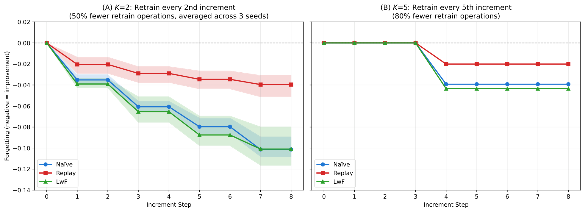
Figure 2 shows the evolution of forgetting across incremental updates for each strategy. The staircase pattern visible in the chart reflects the periodic retraining schedule, where model updates occur only at every K-th increment.

Key observations from the dynamics of forgetting:

Consistent improvement across increments: All of the strategies provided more and more negative values as we moved through the increments of the training process. This shows that through instance-incremental learning (with fixed classes), the model can continually enhance representation.

Naïve and LwF show the strongest improvement trajectories: Both Naïve fine-tuning and LwF have provided the steepest improvements across the increments (−10% by the last increment). Both of these approaches leverage data in a continuous fashion. Naïve does benefit from working with an unconstrained adaptation on samples, while LwF does benefit from the use of regularisation.

Plateau periods between updates: There are flat periods between increments where no retraining takes place. The flat areas between odd and even increments confirm the fact that changes to the performance are due to whether the model was updated.

Forgetting magnitude depends on training amount, not skip duration: An important observation is that different retraining frequencies show similar forgetting magnitudes after their respective first retraining events. For instance, $K=2$ at $r=2$ and $K=5$ at $r=5$ both exhibit approximately −4% forgetting despite $K=5$ skipping training across more increments. This occurs because our periodic retraining strategy trains only on the current increment’s data at each retraining event, not on accumulated data from skipped increments. Thus, both $K=2$ at $r=2$ and $K=5$ at $r=5$ train on a single increment, yielding comparable model updates. The key differentiation lies in computational efficiency: $K=5$ achieves 80% training cost reduction by skipping four increments, while $K=2$ achieves 50% reduction by skipping one increment. This design reflects IoT edge constraints where devices have limited storage and process only the most recent data batch rather than accumulating historical increments.

5.3. Computational Efficiency Analysis

Table 7. Computational efficiency and retraining overhead of periodic retraining, measured directly on the NVIDIA P100. Mixed-precision training enabled direct measurement of the $K=1$ baseline (previously infeasible due to memory limits). “Retrain Ops” is the number of cloud retraining events over the 9-increment schedule; peak GPU memory and estimated training FLOPs are for the naïve strategy (seed 42); runtimes are naïve wall-clock. The exported model is 11.48 MB (FP16, 5.74 M parameters); the LwF teacher copy adds 22.96 MB and the replay buffer 98.87 MB of transient host/GPU overhead during retraining.

Configuration	Retrain Ops	Compute Reduction	Peak GPU/FLOPs	Naïve Runtime
$K=1$ (every increment)	9	– (baseline)	4854 MB/$1.54\times {10}^{15}$	3379 s
$K=2$ (every 2nd)	4	∼50%	2925 MB/$1.01\times {10}^{15}$	1149 s
$K=5$ (every 5th)	1	∼80%	4790 MB/$6.82\times {10}^{14}$	774 s

compares the computational efficiency of periodic retraining against the directly measured $K=1$ baseline of retraining after every increment.

The periodic retraining strategy achieves substantial efficiency gains. With $K=2$, the number of retraining operations is reduced from nine to four (∼50%), and the directly measured naïve wall-clock runtime falls from 3379 s ($K=1$) to 1149 s—a 66% reduction that exceeds the operation-count reduction because per-update cost is broadly similar across increments. At $K=5$, a single retraining event yields a 77% runtime reduction (774 s). Estimated training FLOPs fall correspondingly ($1.54\times {10}^{15}$→$1.01\times {10}^{15}$→$6.82\times {10}^{14}$ for $K=1,2,5$). Peak GPU memory does not decrease monotonically with K, as it is governed by the per-event batch and buffer footprint rather than the number of events; the ∼4.8 GB peaks for naïve $K=1$/$K=5$ remain well within the 16 GB budget under mixed precision. This compute reduction is beneficial for field deployments where the availability of computing resources is restricted and scheduling changes to existing models must accommodate other operational requirements.

5.4. Converged-Base Control

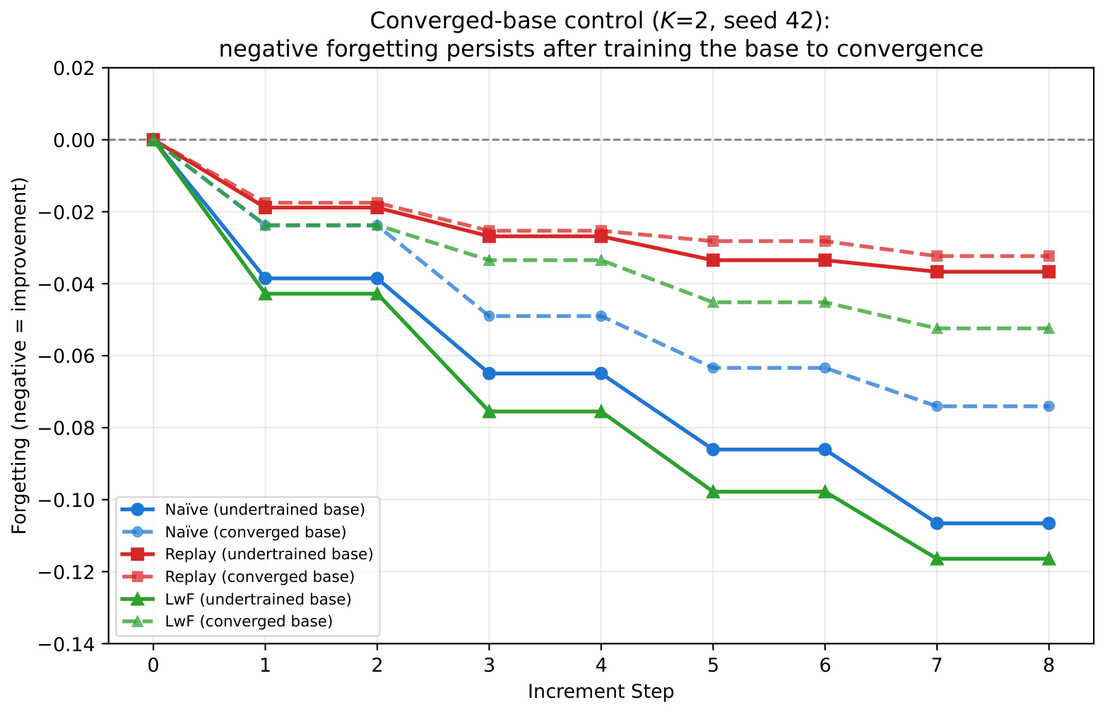
A central question is whether the observed negative forgetting is an intrinsic property of the instance-incremental scenario or an artefact of an undertrained base model that simply has room to improve on any additional data. To disentangle these, we trained the base model to convergence (up to 40 epochs, early-stopped on training loss), raising base accuracy from $a_0=6.08\%$ (8-epoch base, seed 42) to $a_0=14.45\%$, and then ran the identical increment schedule. If negative forgetting were purely a subconvergence carryover effect, it should vanish once the base is converged.

As shown in

Table 8. Converged-base control ($K=2$, seed 42): Final forgetting under an undertrained ($a_0=6.08\%$) versus a converged ($a_0=14.45\%$) base. Negative forgetting persists under the converged base for all strategies, confirming a genuine instance-incremental effect; the reduced magnitude indicates that subconvergence contributes only partially.

Strategy	Undertrained ${\mathit{F}}_{\mathit{R}}$	Converged ${\mathit{F}}_{\mathit{R}}$	Converged Mean $\overline{\mathit{F}}$
Naïve	−10.66%	−7.41%	−4.67%
Replay	−3.67%	−3.23%	−2.29%
LwF	−11.64%	−5.24%	−3.44%

and Figure 3, negative forgetting persists across all three strategies after the base is trained to convergence. The effect attenuates—most notably for LwF, roughly halving—which shows that part of the improvement under the eight-epoch base does reflect continued convergence on a data-starved model. However, the effect does not disappear: final forgetting remains clearly negative (e.g., naïve −7.41%, and −11.84% at $K=1$), demonstrating that instance-incremental reinforcement of existing decision boundaries is a genuine contributor and not merely an initialisation artefact. Both mechanisms therefore operate, with the intrinsic instance-incremental effect dominating for naïve and replay. This control directly addresses the concern that the headline finding might be an artefact of the short base schedule.

5.5. Cumulative-Increment Ablation

We further evaluated a cumulative variant in which, at each retraining event ($r\mathrm{mod}K=0$), the model trains on all increments accumulated since the previous event rather than on the current increment alone. Under $K=2$ (seed 42), cumulative retraining deepens the improvement—naïve final forgetting moves from −10.66% to −15.88% and LwF from −11.64% to −16.64%—because each event sees roughly twice the data. However, this comes at a disproportionate cost: naïve runtime rises from 1149 s to 3083 s (∼2.7×) and LwF from 1399 s to 2188 s, and the cumulative buffer increases edge storage and OTA-staging requirements proportionally to K. Replay is largely unaffected (−3.67% to −3.88%), as it already rehearses historical exemplars. Because the single-increment strategy attains most of the benefit at a fraction of the compute, memory, and bandwidth cost, we retain it as the edge-appropriate default while noting the cumulative variant as an option where retained-class accuracy is paramount and resources permit.

5.6. Baseline Model Performance

To contextualise the continual learning results and demonstrate practical deployment viability, we trained a baseline MobileNetV2 model on the full dataset without incremental constraints [42]. MobileNetV2 is used consistently across all experiments to ensure fair comparison between continual learning strategies and the baseline.

Table 9. Baseline MobileNetV2 model performance on held-out test set (no incremental learning).

Metric	Value
Number of Classes	2719
Test Set Size	60,633
Top-1 Accuracy	26.68%
Top-5 Accuracy	45.75%
Top-10 Accuracy	54.07%
Macro F1-Score	0.2591
Weighted F1-Score	0.2645

presents the test set performance.

The accuracy of the baseline is much greater than that of the continual learning experiments (26.68% versus 7–10% for top-1) due to differences between training on full data versus conducting instance-incremental training. It is important to contextualise these absolute accuracy values against the scale of the classification task. Prior Vietnamese plant studies report 88–99% accuracy on VNPlant-200 [4,6], but that dataset contains only 200 species. Our task spans 2719 fine-grained species—over 13 times more classes—where many species within the same genus share highly similar visual features. At this scale, the random-chance baseline is approximately 0.037% (1/2719), meaning the 26.68% top-1 accuracy represents a 720-fold improvement over random guessing.

Moreover, for large-scale species identification, top-k accuracy is the more operationally relevant metric because practical identification workflows present users with a ranked shortlist of candidate species rather than a single prediction. This ranked candidate paradigm is well established in large-scale plant identification systems such as Pl@ntNet [2] and the PlantCLEF evaluation campaigns [39], where mean reciprocal rank and top-k retrieval metrics are standard. Our model’s 54.07% top-10 accuracy means that the correct species appears in the candidate list more than half the time, providing substantial practical value for field users who can apply their own domain knowledge to select from the shortlist. This baseline has been successfully implemented to provide identification of Vietnamese medicinal plants within the Med Herb Lens Android app.

6. Discussion

6.1. Interpretation of Results

The observation of negative forgetting across all strategies can be attributed to several factors specific to the instance-incremental setting. Unlike class-incremental learning, where new output neurons introduce competing gradients, instance-incremental learning keeps the architecture fixed; new instances reinforce existing decision boundaries rather than displacing them. With fixed classes, each increment adds training data for already-known classes, allowing per-class representations to improve rather than competing for finite model capacity. With 2719 classes, every mini-batch contains diverse gradients, providing implicit multi-task regularisation that promotes class-invariant features and discourages overfitting to recent instances. An important caveat is that the base model was trained on only 20 images per class for eight epochs, achieving 6–10% top-1 accuracy—far below the 26.68% top-1 accuracy of the full-data baseline. Under these conditions, the model has substantial capacity for improvement from any additional training data, regardless of strategy. To determine whether the observed negative forgetting therefore reflects continued convergence on a data-starved model rather than a property of instance-incremental learning, we conducted a converged-base control (Section 5.4): the base was trained to convergence ($a_0$ raised from 6.08% to 14.45%) before running the identical increment schedule. Negative forgetting persisted for all strategies (e.g., naïve final forgetting −7.41% at $K=2$ and −11.84% at $K=1$), though attenuated relative to the undertrained base. We therefore conclude that both mechanisms contribute—a genuine instance-incremental reinforcement effect and a smaller subconvergence carryover—with the intrinsic effect dominating for naïve and replay. The headline finding is thus not an artefact of the short base schedule.

The smaller benefit of experience replay relative to the other two strategies, in turn, can be understood through three observations. In an instance-incremental setting, representations are improving naturally as new data arrives. The replay buffer, however, holds a fixed selection of earlier examples that quickly fall behind the model’s evolving feature space. Sampling from such a buffer reintroduces stale representations of the same classes and can slow, rather than reinforce, the model’s improvement trajectory. With 10 samples per class across 2719 classes (about 27,000 examples total), the buffer captures only a small fraction of the within-class visual diversity. Doubling the buffer to 20 samples per class triggered out-of-memory errors on the 16 GB GPU—a concrete illustration of the scalability challenges replay-based methods face at fine-grained scale. The replay mechanism adds computational overhead (buffer management, additional training samples), but in the instance-incremental scenario where forgetting is not the primary challenge, this overhead does not translate to performance gains. The two new experiments reinforce this account: in the cumulative-increment ablation (Section 5.5) replay is essentially unchanged (−3.67% to −3.88%) despite each event training on roughly twice the data, and in the converged-base control (Section 5.4) it again moves least among the three strategies—both consistent with a buffer whose stale exemplars contribute little once representations are already strong, rather than with mere sampling noise.

Finally, because all strategies now branch from an identical base checkpoint, they share the same base accuracy within a seed; LwF’s advantage is therefore expressed in its incremental trajectory rather than in base accuracy. Its trajectory is comparable to naïve fine-tuning, while incurring additional computational overhead from dual forward passes for teacher–student distillation. In instance-incremental scenarios where the dominant dynamic is improvement rather than forgetting, this overhead is not clearly justified, and naïve fine-tuning offers a simpler and equally effective alternative for resource-constrained deployments.

6.2. Practical Deployment Guidelines

Based on our experimental findings, we offer the following recommendations for deploying continual learning as the model-update component of edge-deployed agricultural IoT pipelines, with particular attention to the resource constraints typical of field and edge settings:

• Consider naïve fine-tuning first: For instance-incremental learning scenarios where new images arrive for existing species, simple fine-tuning is effective and shows strong improvement over time. Avoid the complexity of replay buffers or distillation unless class-incremental updates (new species) are anticipated. Naïve fine-tuning also avoids the additional memory overhead of maintaining replay buffers or teacher models, which is critical when GPU memory is limited (e.g., 16 GB on our NVIDIA P100).
• Use periodic retraining to manage resources: Retraining every K ($K=2$ to 5) new data increments reduces the computational cost of retraining by 50–80% while maintaining comparable performance improvements over time relative to retraining after every increment. In cloud and edge environments, this translates into fewer GPU hours per update (lower energy and monetary cost) and proportionally smaller cumulative OTA bandwidth across the device fleet. Updates can be scheduled during off-peak windows or while devices are connected to power and Wi-Fi.
• Avoid oversized replay buffers at scale: For thousands of fine-grained classes, large replay buffers may exceed memory constraints. Our experiments showed that increasing buffer size from 10 to 20 samples per class caused out-of-memory errors with 2719 classes on 16 GB GPU memory. Developers should budget memory requirements as approximately $B\times C$ images (where B is buffer size per class and C is the number of classes) and verify feasibility before deployment.
• Monitor improvement continuously: Maintain a held-out evaluation set drawn from the original data to track model behaviour as time progresses. In instance-incremental settings, the expectation is performance improvement after retraining rather than forgetting; an automated monitor can use this to gate OTA distribution, releasing a new model only when its evaluation accuracy meets or exceeds the previous version, and avoiding unnecessary cloud retraining cycles when sufficient new data has not yet accumulated.
• Match update frequency to deployment realities: The choice of K determines update cadence and, by extension, OTA bandwidth, per-device update energy, and how quickly new data influences predictions. We discuss specific cadence implications in Section 6.3.3; our experiments with $K=2$ demonstrate a reasonable balance between responsiveness and resource economy for crowdsourced agricultural IoT settings, particularly in rural deployments where cellular connectivity is intermittent.

6.3. IoT System Architecture and Model Lifecycle

The continual learning experiments described above are intended not as standalone results but as the model-update component of an end-to-end agricultural IoT system. This subsection situates the work within that system, describes the three-tier architecture that connects edge inference to periodic retraining, and discusses the over-the-air (OTA) update pathway and its associated connectivity assumptions.

6.3.1. Three-Tier Edge–Gateway–Cloud Architecture

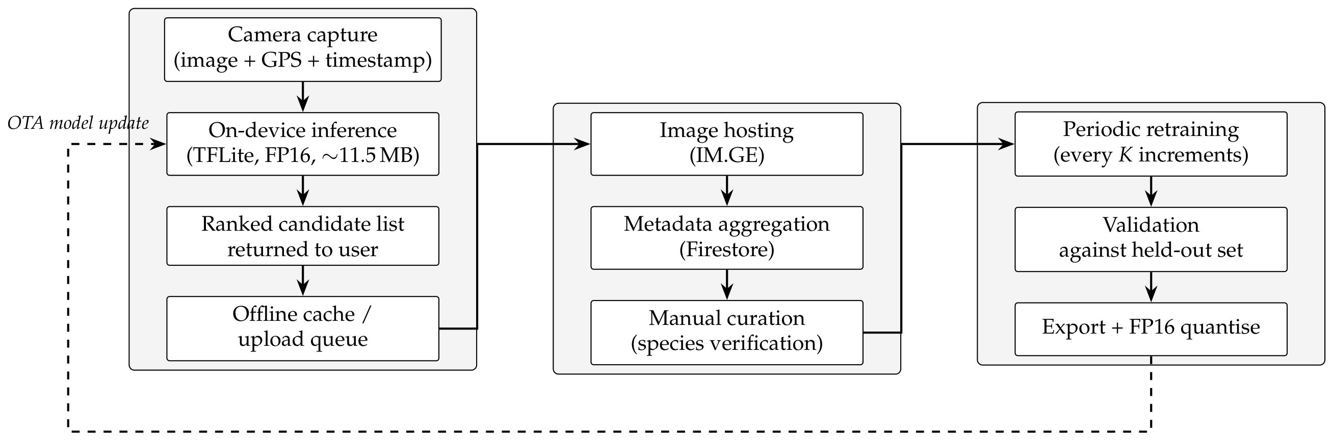
Figure 4 illustrates the three-tier architecture connecting on-device inference, crowdsourced observation upload, and cloud-side periodic retraining. This structure is consistent with the edge–cloud sensing systems reviewed by Vuilliomenet et al. [9] for biodiversity monitoring and with the on-device continual learning patterns surveyed by Lourenço et al. [37] for IoT data streams.

The edge tier corresponds to user smartphones running the Med Herb Lens application. Each device performs on-device inference using a TensorFlow Lite (FP16-quantised, ∼11.5 MB) MobileNetV2 model, returns a ranked candidate list to the user, and—when an image is contributed back—caches the image together with its GPS coordinates and timestamp in a local upload queue. The cache decouples observation capture from network availability, which is essential in rural agricultural settings.

The gateway tier handles aggregation. Image data are uploaded to a hosted image service (currently IM.GE), and structured metadata (image identifier, GPS, timestamp, user-supplied label corrections) are written to a cloud document store (Firestore). At present, a manual curation step verifies species labels before observations enter the training pool; we discuss the implications of this in Section 6.3.3 below.

The cloud tier performs the periodic retraining studied in this paper. At each scheduled retraining event, the new accumulated training data is incorporated into the model using one of the continual learning strategies evaluated in Section 5; the candidate model is validated against the held-out evaluation set; and, on passing validation, it is exported, FP16-quantised, and pushed to edge devices as an OTA update. This pathway turns the algorithmic findings of this paper—that periodic retraining with $K=2$ preserves accuracy at substantially reduced compute—into operational savings in cloud GPU hours, OTA bandwidth, and edge-device update frequency.

6.3.2. Edge Tier: Med Herb Lens Deployment

The baseline model described in Section 5.6 has been deployed in the Med Herb Lens application, currently published on Google Play. The app is built on the prototype architecture described in our earlier work [43], which combines on-device TensorFlow Lite inference with a Firebase-backed knowledge base and offline-capable contribution queue. FP16 post-training quantisation reduces the deployed model to approximately 11.5 MB while preserving inference accuracy, allowing the model to ship within an Android application bundle of practical size for distribution over mobile networks. The user takes a photograph of a plant; the model returns a ranked list of candidate species with confidence scores. This ranked-candidate paradigm aligns with the 54.07% top-10 accuracy of the underlying baseline, meaning the correct species appears within the top ten candidates more than half the time, and the user applies their own botanical knowledge to make the final selection.

On-device benchmark: To characterise the edge tier empirically, we benchmarked the deployed model on three Android devices spanning low-end to mid-range hardware, representative of the device profile typical of rural Vietnamese deployments. For each device we measured cold-start time (median of five app launches, from icon tap to first prediction), per-image inference latency (median over 50 inferences after a 10-image warmup), peak RAM during inference (Android Studio Profiler live telemetry), and battery cost normalised to a per-100-inferences figure derived from the number of consecutive inferences required to register a 1% battery drop with airplane mode enabled and screen brightness at 50%.

Table 10. Edge-tier on-device benchmark for the deployed Med Herb Lens model (MobileNetV2, FP16 TensorFlow Lite, 11.5 MB on disk) on three representative Android devices. Cold-start times are medians of five launches; inference latency is the median over 50 inferences after a 10-image warmup; peak RAM is measured via Android Studio Profiler; battery cost is normalised to a per-100-inferences figure derived from the number of inferences required to register a 1% battery drop with the screen on, airplane mode enabled, and brightness at 50%.

Device	SoC	RAM	Android	Cold Start (s)	Inference Latency (ms)	Peak RAM (MB)	Battery/100 Inf. (%)
OPPO A60	Snapdragon 680	8 GB	14	6.58	201.4	286.3	0.045
Xiaomi Redmi Note 12	Snapdragon 685	8 GB	15	6.90	883.9	423.8	0.077
Realme C21-Y	Unisoc T610	4 GB	11	9.03	1029.7	327.8	0.040

summarises the results.

Three observations follow from the benchmark: First, on-device inference is operationally feasible across all three devices: even on the lowest-spec hardware (Realme C21-Y with 4 GB RAM and an entry-level Unisoc T610 SoC), inference completes in roughly one second per image, which is acceptable for an interactive identification workflow where the user composes a photograph and waits for a ranked list. Second, peak inference-time RAM stays well below 500 MB on all devices, comfortably within the working-set budget of even 4 GB-class phones. Third, the per-100-inferences battery cost is small in absolute terms—between 0.04% and 0.08%—meaning that a typical day of intensive field use (e.g., 100–200 identifications) consumes well under 1% of a 5000 mAh battery on inference alone, with the remaining energy headroom available for camera capture, display, and observation upload. The faster per-inference time on the OPPO A60 relative to the Xiaomi Redmi Note 12, despite the SoCs being closely matched on synthetic benchmarks, is most plausibly attributable to differences in the default TensorFlow Lite delegate selected by each vendor’s OS image (e.g., NNAPI versus CPU-only fallback); we did not control for delegate selection in this study.

Scope of the benchmark: Table 10 characterises the baseline MobileNetV2 model currently deployed in the Med Herb Lens application (Section 5.6). Because the periodic retraining strategy investigated in this work preserves the MobileNetV2 architecture and the FP16 quantisation pipeline, the inference profile reported here applies equally to any model produced by the retraining loop; the strategy modifies which weights are deployed, not the architectural envelope within which inference occurs. End-to-end deployment of a periodically retrained model is identified as a near-term engineering step (Section 6.5).

Positioning relative to other edge ML systems:

Table 11. Positioning of the present work alongside representative edge-deployed plant/ecological classification systems and on-device continual learning research. “Deployed” indicates whether the system was shipped beyond a research prototype to a real edge target; “CL pipeline” indicates whether the work includes a continual learning component for model updates over time. The bold row denotes the present work. “AR1*” is the name of a continual learning method (a native-rehearsal variant of AR1); the asterisk is part of the method name, not a footnote marker.

System	Domain	Classes	Architecture	Model Size	Edge Platform	Deployed	CL Pipeline
Guan et al. [35]	Plant disease (PlantVillage)	38	Dise-Efficient (custom)	13.3 MB	Lightweight (general)	No	No
Zhou et al. [36]	Field crop disease	8	REM-ShuffleNetV2	4.40 M params	Lightweight (general)	No	No
Mohanty et al. [3]	Plant disease (PlantVillage)	38	AlexNet/ GoogLeNet	—	Smartphone (proposed)	No	No
Pl@ntNet [2]	General plant ID	1000 s+	CNN (cloud-assisted)	N/A (cloud)	Smartphone	Yes	No
Pellegrini et al. [44]	Object recognition (CORe50)	50	MobileNetV1 + AR1*	—	Smartphone (Android)	Yes (research)	Yes (on-device)
Tran et al. (KES 2025) [43]	Vietnamese medicinal plants (prototype)	7	EfficientNetB0	<10 MB	Smartphone (Android)	Yes	No
This work	Vietnamese medicinal plants	2719	MobileNetV2 (FP16)	11.5 MB	Smartphone (Android)	Yes (Google Play)	Yes (periodic retraining)

situates this work among representative edge-deployed plant and ecological classification systems and on-device continual learning research. The dimensions chosen highlight the combination of properties that distinguishes the present work: large class count, deployed (rather than benchmark-only) edge model, agricultural IoT framing, and inclusion of a continual learning pipeline.

The combination of properties in the bottom row—a deployed edge-tier model serving thousands of fine-grained classes, paired with a continual learning pipeline designed for the IoT model lifecycle—is, to the best of our knowledge, not jointly achieved by any prior plant identification or on-device continual learning system. Pellegrini et al. [44] is the closest analogue in deploying continual learning on a real Android device, but their study uses a 50-class object-recognition benchmark and focuses on personalisation rather than agricultural IoT. Pl@ntNet operates at large class scale but is fundamentally a cloud-assisted system rather than an edge-resident model, and it does not employ continual learning for its on-device component.

6.3.3. OTA Model Updates and Connectivity Assumptions

The cloud-to-edge pathway shown in Figure 4 is the operational expression of our periodic retraining strategy. Each retraining event yields one OTA model update; the choice of K therefore directly determines update frequency and, by extension, the bandwidth, energy, and storage costs incurred across the device fleet.

For the deployed FP16 model (∼11.5 MB per update), the choice of K has significant operational implications. With $K=2$ and an accumulation rate of one increment per fortnight, an OTA push occurs roughly once per month. Aggregated over a notional fleet of N active devices, this scales to bandwidth and energy budgets that are linear in N and inversely proportional to K. Periodic retraining with larger K values would translate into proportionally smaller cumulative OTA bandwidth and per-device energy expenditure for model updates—a non-trivial concern in rural deployments where users may be on metered cellular connections.

The architecture is also explicitly designed for intermittent connectivity. The edge-tier upload queue (Figure 4) caches observations when the device is offline and synchronises them once a network connection is available. OTA updates are similarly opportunistic: on the receiving side, the application checks for a new model on launch when a network is reachable and downloads it preferentially over Wi-Fi to avoid imposing cellular costs on the user. These design choices follow established patterns for IoT edge devices operating under unreliable connectivity [37] and reflect the rural-deployment assumptions identified by earlier surveys of agricultural deep learning [7].

Field deployment also introduces data-quality considerations distinct from algorithmic accuracy. Edge-captured images vary significantly under natural lighting and weather, and contributing users may photograph plants at different growth stages, from varying angles, and at varying spatial scales (whole plant, leaf cluster, individual leaf). Geotagging quality depends on the device’s location subsystem, and timestamp metadata can be coarsened by user privacy settings. The periodic retraining loop is precisely the mechanism by which the model adapts to these field-realistic conditions over time, rather than remaining frozen on the comparatively uniform GBIF reference imagery used for the initial baseline.

It is important to be precise about the current state of automation. The pipeline shown in Figure 4 is fully designed and the edge and gateway tiers are operationally deployed: the application is published on Google Play, image uploads to IM.GE function end-to-end, and metadata aggregation in Firestore is active. The cloud retraining step itself, however, is currently performed manually using the Kaggle notebook released alongside this paper [42]—contributed images are downloaded from IM.GE, manually verified, and integrated into the training set, and a retrained model is exported and uploaded for OTA distribution. The application has not yet been promoted to the Vietnamese user community, so observation upload volume is presently low, and full automation of the retraining trigger has not yet been required. Closing this gap—an automated retraining trigger that fires every K accumulated, verified increments—is a near-term engineering objective that the present empirical study is intended to support. We stress that automating the compute trigger is distinct from automating the data verification it depends on: expert verification of crowdsourced images guards against safety-critical errors such as mislabelled toxic look-alikes, and this human-in-the-loop step—not the trigger—becomes the dominant bottleneck as the user base grows. We therefore envisage scaling verification through a tiered, semi-automated scheme: confidence/uncertainty filtering to auto-accept high-agreement submissions and route only ambiguous ones to experts; per-contributor trust scores; and expert-consensus adjudication reserved for toxic or frequently-confused species. Only submissions clearing verification enter the retraining pool.

Beyond direct user identification, the architecture also supports several broader ecological workflows. Extension workers and field surveyors can use the application during biodiversity assessments and contribute locally collected specimens back into the training pipeline; conservation programmes can systematically catalogue medicinal plant populations through aggregated user observations; and herbal supply chains can use it as a secondary check to reduce misidentification at collection points. In each case, verified observations feed back into the periodic retraining loop described in this study, gradually improving model accuracy over time.

6.4. Limitations

This study has several limitations that should be considered when interpreting results, which we group below by methodological scope, computational constraints, and the maturity of the deployed pipeline.

Scope and methodology: Our experiments consider only instance-incremental learning where the class set is fixed; class-incremental scenarios (adding new species over time) present different challenges and may show different patterns, including actual catastrophic forgetting. To maintain consistency across all experiments, MobileNetV2 was used as the sole base architecture, and performance differences in alternative architectures (e.g., Vision Transformers or larger backbones) may yield different results. The experiments also use a partitioned static dataset to simulate incremental arrival, whereas real-world crowdsourced datasets may contain different temporal patterns and distribution shifts in addition to variation in image quality. More broadly, the present study characterises the cloud-tier retraining step in a controlled simulation; several gaps remain before large-scale deployment: increments arrive on a fixed schedule with balanced per-class counts rather than the bursty, long-tailed, geographically clustered arrival typical of crowdsourcing; labels are verified offline rather than under live load; and inter-increment distribution shift (season, device, region) is not explicitly modelled. The deployed edge and gateway tiers (Section 6.3.3) already exercise the data pathway end-to-end, but validating these findings under real arrival patterns and user-contributed label noise remains future work. Additionally, our periodic retraining implementation trains only on the current increment at each retraining event rather than accumulating skipped increments; we evaluated the alternative cumulative strategy (training on all pending increments when $r\mathrm{mod}K=0$) in Section 5.5, finding that it deepens the improvement but at a disproportionate compute, memory, and OTA-bandwidth cost, which is why the single-increment strategy is retained as the edge-appropriate default.

Computational constraints: Several of our design choices were driven by the 16 GB VRAM ceiling of the NVIDIA P100 GPU used for experiments. In the original submission we were unable to test $K=1$ (retraining every increment); in this revision, enabling mixed-precision (FP16) training reduced peak memory enough to measure the $K=1$ baseline directly, confirming the efficiency claim empirically (a 66% naïve wall-clock reduction for $K=2$; Section 5.3) rather than relying on the operation-count argument alone. Similar memory pressure prevented systematic testing of larger replay buffers (e.g., 20 samples per class), which itself serves as a concrete example of the scalability challenges replay-based approaches face at fine-grained scales of thousands of classes. We report three random seeds (42, 123 and 456) for the main $K=2$ configuration; a third seed had produced an out-of-memory error under the original settings, and enabling mixed-precision training made it feasible to complete. We report Student’s t 95% confidence intervals for final forgetting in Section 5.1; all three exclude zero, so the negative-forgetting effect is significant, but with only three seeds these intervals are necessarily wide and rest on an approximate-normality assumption that cannot be verified at $n=3$. Rather than over-interpreting a small-sample variance estimate, we therefore emphasise that the direction (negative forgetting) and the ordering of strategies (naïve ≈ LwF ≫ replay) are consistent across all three seeds, and are further corroborated by the $K=5$ and converged-base control runs.

Interpretation of accuracy: The difference in accuracy between the continual learning experiments (7–10% top-1 accuracy) and the baseline model (26.68% top-1 accuracy) demonstrates the constrained nature of instance-incremental learning when only a limited number of images per class are available at each increment. However, these figures should be interpreted in light of the 2719-class scale (where random chance is 0.037%) and the ranked candidate identification paradigm: the baseline model’s 54.07% top-10 accuracy indicates that the correct species appears in the shortlist more than half the time, which is the operationally relevant metric for deployed plant identification systems.

Pipeline maturity and benchmark coverage: As described in Section 6.3.3, the cloud-tier retraining step is currently triggered manually through a Kaggle notebook rather than by an automated event-driven trigger over accumulated edge contributions. The architecture supports full automation, and the periodic retraining strategy evaluated here is the algorithmic basis for that automation, but the end-to-end loop has not yet been exercised under real user load; the findings of this study are intended to inform the operational parameters (K, strategy, validation thresholds) of the automated trigger when it is deployed. Similarly, the on-device benchmark in Section 6.3.2 (Table 10) covers three Android devices spanning low-end to mid-range hardware. While this range is representative of devices typical in rural Vietnamese deployments, it does not include flagship devices, tablets, or non-Android edge platforms; performance on those targets, and the influence of vendor-specific TensorFlow Lite delegate selection, remain to be characterised systematically. Specifically, the latencies in Table 10 were obtained under each device’s default delegate resolution (NNAPI where available, with CPU fallback) rather than a single forced delegate, so the cross-device spread partly reflects heterogeneous NNAPI/DSP support rather than model cost alone. We report them as indicative of the realistic out-of-the-box experience on rural hardware; pinning the delegate (NNAPI, GPU, Hexagon DSP, or CPU) per device to isolate model-intrinsic latency is a clear next step, and this edge-side spread does not affect the cloud-tier retraining findings that are the paper’s focus.

6.5. Future Directions

This work opens several directions for future research.

• Convergence and architecture robustness: The converged-base control (Section 5.4) establishes that negative forgetting persists beyond subconvergence for a single seed; extending this control across multiple seeds and to larger or transformer-based backbones (e.g., Vision Transformers, MobileViT) would further test the generality of the effect.
• Class-incremental scenarios: Extend the evaluation to class-incremental learning, where new species are added over time and forgetting is expected to be more pronounced. The fixed 2719-way MobileNetV2 head cannot admit new classes without structural change; candidate adaptations—each trading off differently against the memory and OTA constraints analysed here—include an extensible head that grows the output layer (low OTA cost, but recency-biased without rehearsal), a prototype/nearest-mean-of-exemplars classifier (iCaRL-style) that avoids resizing the head at the cost of a growing prototype store, and dynamic output expansion with parameter isolation (strongest protection, but parameters and OTA payload scale with expansions). Recent on-device incremental-learning frameworks confirm the practicality of these adaptations under edge constraints; for instance, LODAP combines a lightweight structural-expansion module, a prototype store, and knowledge distillation to learn new classes on-device while roughly halving model complexity [45].
• Federated continual learning: Investigate federated continual learning (FCL) for the agricultural IoT setting. The architecture in Figure 4 is currently centralised: contributed images and metadata leave the edge device. A federated formulation would instead train model updates locally on each edge device or on a regional gateway and aggregate only model parameters at the cloud tier, preserving the privacy of contributed images and reducing OTA-direction bandwidth at the cost of higher per-device energy and compute. Recent surveys situate FCL within the IoT edge-AI research frontier [37], including a comprehensive 2024 survey dedicated to federated continual learning for Edge-AI [46], and the periodic retraining cadence studied here translates naturally into a federated aggregation cadence.
• Uncertainty-aware curation: Integrate uncertainty quantification into the process when determining which images should undergo expert verification prior to being added to training datasets.
• Multi-modal learning: Extend the model to incorporate textual descriptions, geographic metadata, and seasonal information alongside images.
• Memory-efficient replay at scale: Build replay strategies that scale to thousands of classes without exceeding device memory boundaries.
• Systematic study of K: Systematically investigate the periodic retraining period across a wider range of K; the $K=1$ baseline is now directly benchmarked (Section 5.3), providing the anchor for these comparisons.
• Wider edge characterisation: Extend the edge-inference characterisation in Section 6.3.2 to a wider device range (including flagships, tablets, and non-Android targets), and use power-instrumented measurement (rather than battery-percentage proxy) to isolate inference energy from screen and SoC idle costs. Systematic study of vendor-specific TensorFlow Lite delegate behaviour (NNAPI, GPU, Hexagon DSP) is also a natural extension, given the substantial cross-device latency variation observed in this study.

7. Conclusions

This study addressed how continual learning can be deployed efficiently and reliably as the model-update component of an agricultural IoT pipeline for large-scale fine-grained medicinal plant identification. Through systematic experiments on a dataset of 2719 species, with cross-seed consistency checks and multiple retraining frequencies, we compared naïve fine-tuning, experience replay, and Learning without Forgetting under a periodic retraining strategy designed for computational efficiency, and situated the findings within an end-to-end edge–gateway–cloud architecture for crowdsourced agricultural IoT.

Our key findings indicate that instance-incremental learning exhibits negative forgetting (performance improvement over time) rather than catastrophic forgetting, with naïve fine-tuning and LwF showing the strongest improvement trajectories (final forgetting of approximately −10%). This result suggests that explicit forgetting mitigation techniques may be unnecessary when new data reinforces existing class representations, although the limited initial training data (20 images per class) may also contribute to the observed improvement pattern.

Furthermore, we demonstrated that periodic retraining with $K=2$ reduces the number of retraining operations by approximately 50% while maintaining competitive performance. In an agricultural IoT model-lifecycle setting, this compute reduction translates directly into proportionally smaller cloud GPU usage, OTA bandwidth, and per-device update energy. A baseline MobileNetV2 model trained on the full dataset achieves 54.07% top-10 accuracy across 2719 species—meaning the correct species appears in the ranked candidate list more than half the time—with a corresponding top-1 accuracy of 26.68% (a 720-fold improvement over random chance at this scale), demonstrating practical viability for edge deployment through ranked candidate identification. This baseline has been successfully deployed via TensorFlow Lite (FP16, ∼11.5 MB) in the Med Herb Lens Android application, which we describe as the edge tier of a three-tier edge–gateway–cloud IoT architecture (Section 6.3); the cloud tier of this architecture is where the periodic retraining strategy investigated here operates.

By addressing the challenges of scalable continual learning in fine-grained plant classification within a deployable IoT pipeline, this work contributes both methodological understanding and actionable deployment guidance—including concrete recommendations on strategy selection, retraining frequency, memory budgeting, and connectivity-aware OTA scheduling—for adaptive machine learning systems in agricultural and field IoT settings. Future work will extend these approaches to class-incremental scenarios where catastrophic forgetting is expected to be more pronounced, to federated continual learning configurations that better suit privacy- and bandwidth-constrained edge deployments, and to multi-modal plant identification systems.

References

1. Mulugeta, A.K.; Sharma, D.P.; Mesfin, A.H. Deep Learning for Medicinal Plant Species Classification and Recognition: A Systematic Review. Front. Plant Sci. 2024, 14, 1286088. [Google Scholar] [CrossRef] [Scilit] [PubMed]
2. Affouard, A.; Goëau, H.; Bonnet, P.; Lombardo, J.-C.; Joly, A. Pl@ntNet App in the Era of Deep Learning. In Proceedings of the ICLR 2017 Workshop Track, Toulon, France, 24–26 April 2017. [Google Scholar]
3. Mohanty, S.P.; Hughes, D.P.; Salathé, M. Using Deep Learning for Image-Based Plant Disease Detection. Front. Plant Sci. 2016, 7, 1419. [Google Scholar] [CrossRef] [Scilit] [PubMed]
4. Nguyen Quoc, T.; Truong Hoang, V. Medicinal Plant Identification in the Wild by Using CNN. In Proceedings of the International Conference on Information and Communication Technology Convergence (ICTC), Jeju Island, Republic of Korea, 21–23 October 2020; pp. 25–29. [Google Scholar]
5. Nguyen Quoc, T.; Truong Hoang, V. VNPlant-200: A Public and Large-Scale Vietnamese Medicinal Plant Image Dataset. Lect. Notes Netw. Syst. 2021, 136, 406–411. [Google Scholar]
6. Nhut, D.T.N.; Tan, T.D.; Quoc, T.N.; Hoang, V.T. Medicinal Plant Recognition Based on Vision Transformer and BEiT. Procedia Comput. Sci. 2024, 234, 188–195. [Google Scholar] [CrossRef] [Scilit]
7. Kamilaris, A.; Prenafeta-Boldú, F.X. Deep Learning in Agriculture: A Survey. Comput. Electron. Agric. 2018, 147, 70–90. [Google Scholar] [CrossRef] [Scilit]
8. Atsumi, K.; Nishida, Y.; Ushio, M.; Nishi, H.; Genroku, T.; Fujiki, S. Boosting Biodiversity Monitoring Using Smartphone-Driven, Rapidly Accumulating Community-Sourced Data. eLife 2024, 13, RP93694. [Google Scholar] [CrossRef] [PubMed]
9. Vuilliomenet, A.; Jones, K.E.; Wilson, D. Future of Edge AI in Biodiversity Monitoring. arXiv 2026, arXiv:2602.13496. [Google Scholar] [CrossRef] [Scilit]
10. Parisi, G.I.; Kemker, R.; Part, J.L.; Kanan, C.; Wermter, S. Continual Lifelong Learning with Neural Networks: A Review. Neural Netw. 2019, 113, 54–71. [Google Scholar] [CrossRef] [Scilit] [PubMed]
11. McCloskey, M.; Cohen, N.J. Catastrophic Interference in Connectionist Networks: The Sequential Learning Problem. Psychol. Learn. Motiv. 1989, 24, 109–165. [Google Scholar] [CrossRef] [Scilit]
12. French, R.M. Catastrophic Forgetting in Connectionist Networks. Trends Cogn. Sci. 1999, 3, 128–135. [Google Scholar] [CrossRef] [Scilit] [PubMed]
13. De Lange, M.; Aljundi, R.; Masana, M.; Parisot, S.; Jia, X.; Leonardis, A.; Slabaugh, G.; Tuytelaars, T. A Continual Learning Survey: Defying Forgetting in Classification Tasks. IEEE Trans. Pattern Anal. Mach. Intell. 2022, 44, 3366–3385. [Google Scholar] [PubMed]
14. Masana, M.; Liu, X.; Twardowski, B.; Menta, M.; Bagdanov, A.D.; van de Weijer, J. Class-Incremental Learning: Survey and Performance Evaluation on Image Classification. IEEE Trans. Pattern Anal. Mach. Intell. 2023, 45, 5513–5533. [Google Scholar] [CrossRef] [Scilit] [PubMed]
15. van de Ven, G.M.; Tolias, A.S. Three Scenarios for Continual Learning. arXiv 2019, arXiv:1904.07734. [Google Scholar]
16. van de Ven, G.M.; Tuytelaars, T.; Tolias, A.S. Three Types of Incremental Learning. Nat. Mach. Intell. 2022, 4, 1185–1197. [Google Scholar] [CrossRef] [Scilit] [PubMed]
17. Rolnick, D.; Ahuja, A.; Schwarz, J.; Lillicrap, T.; Wayne, G. Experience Replay for Continual Learning. Adv. Neural Inf. Process. Syst. 2019, 32, 348–358. [Google Scholar]
18. Li, Z.; Hoiem, D. Learning without Forgetting. IEEE Trans. Pattern Anal. Mach. Intell. 2018, 40, 2935–2947. [Google Scholar] [CrossRef] [Scilit] [PubMed]
19. Rusu, A.A.; Rabinowitz, N.C.; Desjardins, G.; Soyer, H.; Kirkpatrick, J.; Kavukcuoglu, K.; Pascanu, R.; Hadsell, R. Progressive Neural Networks. arXiv 2016, arXiv:1606.04671. [Google Scholar]
20. Mallya, A.; Lazebnik, S. PackNet: Adding Multiple Tasks to a Single Network by Iterative Pruning. In Proceedings of the IEEE Conference on Computer Vision and Pattern Recognition (CVPR), Salt Lake City, UT, USA, 18–23 June 2018; pp. 7765–7773. [Google Scholar]
21. Nguyen, V.H.; Ngo, L.H.H. Automatic Plant Image Identification of Vietnamese Species Using Deep Learning Models. Int. J. Eng. Trends Technol. 2020, 68, 25–31. [Google Scholar] [CrossRef] [Scilit]
22. Dat, T.T.; Le Thien Vu, P.C.; Truong, N.N.; Anh Dang, L.T.; Thanh Sang, V.N.; Bao, P.T. Leaf Recognition Based on Joint Learning Multiloss of Multimodel Convolutional Neural Networks: A Testing for Vietnamese Herb. Comput. Intell. Neurosci. 2021, 2021, 5032359. [Google Scholar] [CrossRef] [Scilit] [PubMed]
23. Zhang, Y.; Sun, W.; Yang, C.; Huang, L.; An, Z.; Feng, W.; Tang, W.; Xu, Y. TCMP-300: A Comprehensive Traditional Chinese Medicinal Plant Dataset for Plant Recognition. Sci. Data 2025, 12, 1166. [Google Scholar] [CrossRef] [Scilit] [PubMed]
24. Read, J.; Bifet, A.; Pfahringer, B.; Holmes, G. Batch-Incremental versus Instance-Incremental Learning in Dynamic and Evolving Data. In Proceedings of the International Symposium on Intelligent Data Analysis (IDA), Helsinki, Finland, 25–27 October 2012; pp. 313–323. [Google Scholar]
25. Wang, L.; Zhang, X.; Su, H.; Zhu, J. A Comprehensive Survey of Continual Learning: Theory, Method and Application. IEEE Trans. Pattern Anal. Mach. Intell. 2024, 46, 5362–5383. [Google Scholar] [CrossRef] [Scilit] [PubMed]
26. Zhou, D.-W.; Wang, Q.-W.; Qi, Z.-H.; Ye, H.-J.; Zhan, D.-C.; Liu, Z. Class-Incremental Learning: A Survey. IEEE Trans. Pattern Anal. Mach. Intell. 2024, 46, 9851–9873. [Google Scholar] [CrossRef] [Scilit] [PubMed]
27. Kirkpatrick, J.; Pascanu, R.; Rabinowitz, N.; Veness, J.; Desjardins, G.; Rusu, A.A.; Milan, K.; Quan, J.; Ramalho, T.; Grabska-Barwinska, A.; et al. Overcoming Catastrophic Forgetting in Neural Networks. Proc. Natl. Acad. Sci. USA 2017, 114, 3521–3526. [Google Scholar] [CrossRef] [Scilit] [PubMed]
28. Zenke, F.; Poole, B.; Ganguli, S. Continual Learning through Synaptic Intelligence. In Proceedings of the International Conference on Machine Learning (ICML), Sydney, Australia, 6–11 August 2017; pp. 3987–3995. [Google Scholar]
29. Li, Z.; Hoiem, D. Learning without Forgetting. In Proceedings of the European Conference on Computer Vision (ECCV), Amsterdam, The Netherlands, 11–14 October 2016; pp. 614–629. [Google Scholar]
30. Shin, H.; Lee, J.K.; Kim, J.; Kim, J. Continual Learning with Deep Generative Replay. Adv. Neural Inf. Process. Syst. 2017, 30, 2990–2999. [Google Scholar]
31. Rebuffi, S.-A.; Kolesnikov, A.; Sperl, G.; Lampert, C.H. iCaRL: Incremental Classifier and Representation Learning. In Proceedings of the IEEE Conference on Computer Vision and Pattern Recognition (CVPR), Honolulu, HI, USA, 21–26 July 2017; pp. 5533–5542. [Google Scholar]
32. Lopez-Paz, D.; Ranzato, M. Gradient Episodic Memory for Continual Learning. Adv. Neural Inf. Process. Syst. 2017, 30, 6467–6476. [Google Scholar]
33. van de Ven, G.M.; Siegelmann, H.T.; Tolias, A.S. Brain-Inspired Replay for Continual Learning with Artificial Neural Networks. Nat. Commun. 2020, 11, 4069. [Google Scholar] [CrossRef] [Scilit] [PubMed]
34. Picek, L.; Šulc, M.; Patel, Y.; Matas, J. Plant Recognition by AI: Deep Neural Nets, Transformers, and kNN in Deep Embeddings. Front. Plant Sci. 2022, 13, 787527. [Google Scholar] [CrossRef] [Scilit] [PubMed]
35. Guan, H.; Fu, C.; Zhang, G.; Li, K.; Wang, P.; Zhu, Z. A Lightweight Model for Efficient Identification of Plant Diseases and Pests Based on Deep Learning. Front. Plant Sci. 2023, 14, 1227011. [Google Scholar] [CrossRef] [Scilit] [PubMed]
36. Zhou, H.; Chen, J.; Niu, X.; Dai, Z.; Qin, L.; Ma, L.; Li, J.; Su, Y.; Wu, Q. Identification of Leaf Diseases in Field Crops Based on Improved ShuffleNetV2. Front. Plant Sci. 2024, 15, 1342123. [Google Scholar] [CrossRef] [Scilit] [PubMed]
37. Lourenço, A.; Rodrigo, J.; Gama, J.; Marreiros, G. On-Device Edge Learning for IoT Data Streams: A Survey. arXiv 2025, arXiv:2502.17788. [Google Scholar] [CrossRef] [Scilit]
38. Tran, T.P.; Din, F.U.; Brankovic, L.; Sanin, C.; Hester, S.M. Viet Medi Species 2026: A Web-Accessible Multilingual Dataset for Vietnamese Medicinal Biodiversity. In Proceedings of the Companion Proceedings of the ACM Web Conference 2026 (WWW Companion ’26), Dubai, United Arab Emirates, 29 June–3 July 2026; ACM: New York, NY, USA, 2026; 8p. [Google Scholar] [CrossRef] [Scilit]
39. Goëau, H.; Bonnet, P.; Joly, A. Overview of PlantCLEF 2023: Image-Based Plant Identification at Global Scale. In Proceedings of the CLEF 2023 Working Notes, Thessaloniki, Greece, 18–21 September 2023. [Google Scholar]
40. Pushpa, B.R.; Shobha Rani, N. DIMPSAR: Dataset for Indian Medicinal Plant Species Analysis and Recognition. Data Brief. 2023, 49, 109388. [Google Scholar] [CrossRef] [Scilit]
41. Hinton, G.; Vinyals, O.; Dean, J. Distilling the Knowledge in a Neural Network. arXiv 2015, arXiv:1503.02531. [Google Scholar]
42. Tran, T. Species-Level-2026: Kaggle Code Notebook. Kaggle. 2026. Available online: https://www.kaggle.com/code/trientran/species-level-2026 (accessed on 10 May 2026).
43. Tran, T.P.; Din, F.U.; Brankovic, L.; Sanin, C.; Hester, S.M. Med Herb Lens: A Prototype AI App for Medicinal Plant Identification. Procedia Comput. Sci. 2025, 270, 2603–2612. [Google Scholar] [CrossRef] [Scilit]
44. Pellegrini, L.; Lomonaco, V.; Graffieti, G.; Maltoni, D. Continual Learning at the Edge: Real-Time Training on Smartphone Devices. In Proceedings of the 29th European Symposium on Artificial Neural Networks, Computational Intelligence and Machine Learning (ESANN 2021), Bruges, Belgium, 6–8 October 2021; pp. 23–28. [Google Scholar] [CrossRef] [Scilit]
45. Duan, B.; Wang, Q.; Liu, D.; Zhou, W.; He, Z.; Miao, S. LODAP: On-device Incremental Learning via Lightweight Operations and Data Pruning. J. Syst. Archit. 2025, 168, 103571. [Google Scholar] [CrossRef] [Scilit]
46. Wang, Z.; Wu, F.; Yu, F.; Zhou, Y.; Hu, J.; Min, G. Federated Continual Learning for Edge-AI: A Comprehensive Survey. arXiv 2024, arXiv:2411.13740. [Google Scholar] [CrossRef] [Scilit]
Figure 1. Representative images from the Viet Medi Species 2026 dataset for four congeneric species of Abelmoschus. Reading across the top row illustrates the fine-grained visual similarity between distinct species, while reading down each column illustrates the variation in field background, lighting, and viewpoint within a single species. This combination of high inter-species similarity and intra-species variability underlies the difficulty of the 2719-class identification task. Images are drawn from the publicly available Viet Medi Species 2026 dataset, whose occurrence records are aggregated from the Global Biodiversity Information Facility (GBIF) under their respective open licences.
Iot 07 00057 g001
Figure 2. Forgetting curves for three continual learning strategies under periodic retraining with K = 2 (model retrained every 2nd increment, 50% fewer retraining operations). Results are averaged across seeds 42, 123 and 456; shaded bands indicate the range between seeds. Negative forgetting values indicate there has been an overall increase in performance instead of a drop. The staircase pattern shows that when there are gaps between retraining, the performance of models does not change. During skipped increments (odd r for K = 2 ), the model maintains frozen weights and exhibits zero forgetting until the next retraining event. Key observation: All three strategies trend increasingly negative (i.e., accuracy improves) as increments accumulate, with naïve and LwF improving most and replay least; at the matched first-retrain point, K = 2 ( r = 2 ) and K = 5 ( r = 5 ) reach comparable forgetting (∼−4%), confirming that update magnitude is governed by per-event data volume rather than the number of skipped increments.
Iot 07 00057 g002
Figure 3. Converged-base control ( K = 2 , seed 42). Solid lines: Undertrained 8-epoch base; dashed lines: base trained to convergence (40 epochs). Negative forgetting persists under the converged base for all strategies, confirming the effect is intrinsic to the instance-incremental setting rather than an artefact of subconvergence, while its reduced magnitude shows subconvergence contributes only in part.
Iot 07 00057 g003
Figure 4. Three-tier edge–gateway–cloud architecture for the agricultural IoT pipeline supporting Med Herb Lens. The edge tier performs on-device inference and queues observations for upload; the gateway tier aggregates uploaded images and metadata; and the cloud tier performs periodic retraining (every K increments, per Algorithm 1), validates the new model, and distributes it back to edge devices via OTA update (dashed arrow). The continual learning experiments in Section 5 characterise the cloud-tier retraining step.
Iot 07 00057 g004