Casimir Forces with Periodic Structures: Abrikosov Flux Lattices

 ,
,  , and
, and 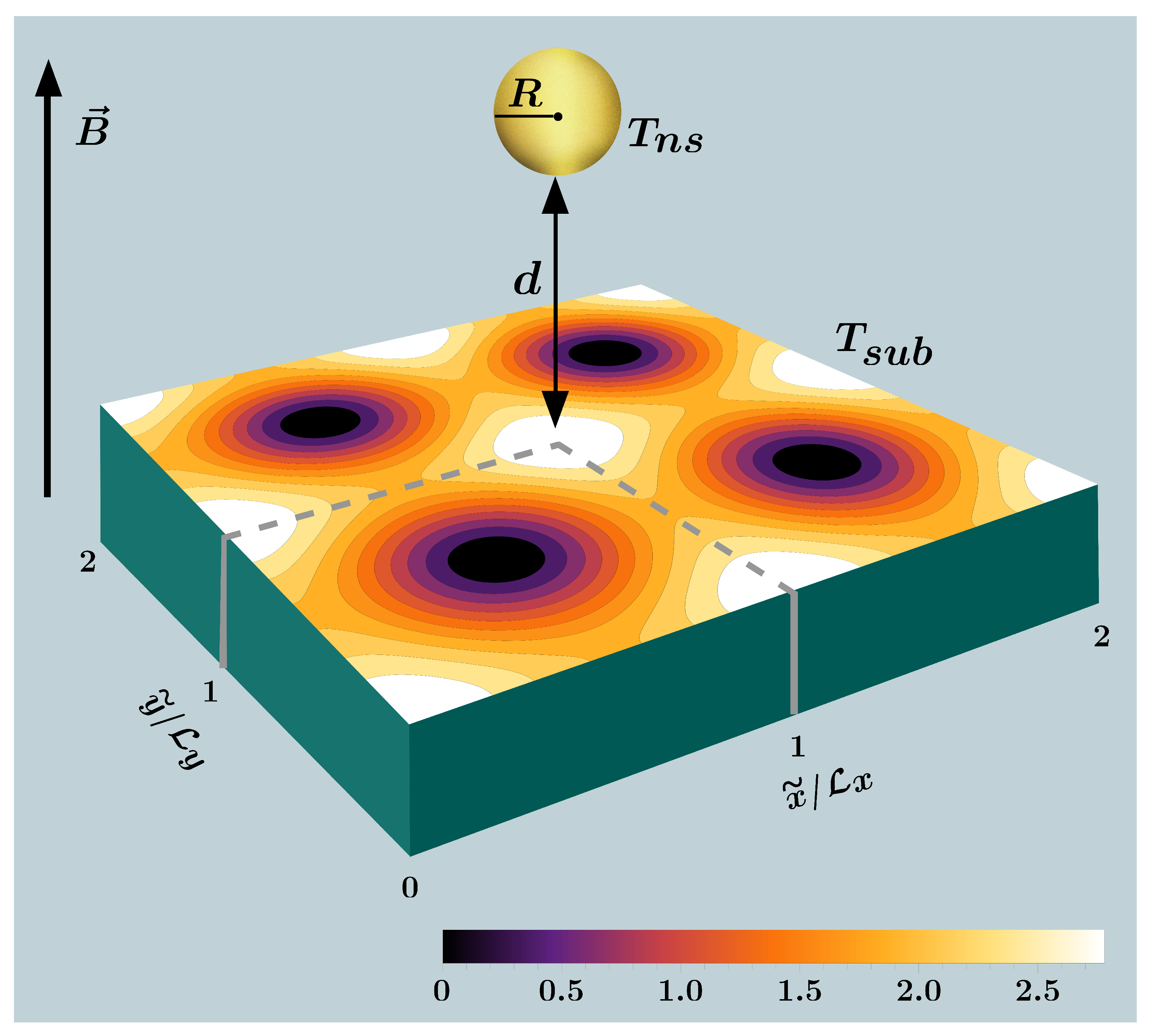
Abstract
1. Introduction
2. Theory and Definitions
2.1. Casimir Force between a Nanosphere and a Planar Substrate
2.2. Ginzburg–Landau Theory and the Optical Response of the YBCO Substrate
2.3. Thermal Properties of the Order Parameter
2.4. YBCO Dielectric Response
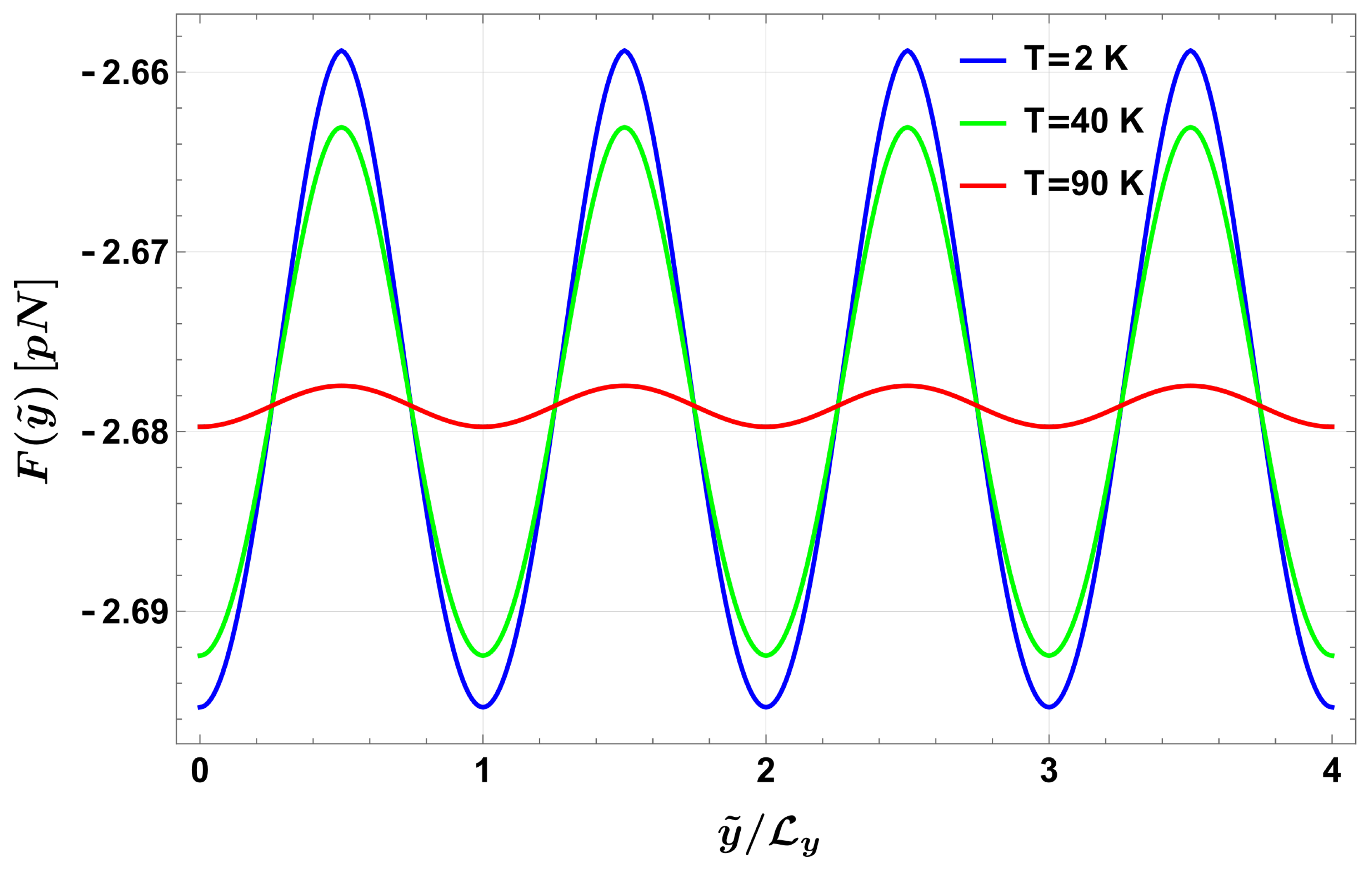
3. Results
4. Discussion and Conclusions
Author Contributions
Funding
Data Availability Statement
Conflicts of Interest
References
- Casimir, H.B.G. On the attraction between two perfectly conducting plates. Proc. Kon. Ned. Akad. Wet. B 1948, 51, 793–795. Available online: https://dwc.knaw.nl/DL/publications/PU00018547.pdf (accessed on 29 January 2024).
- Lifshitz, E.M. The theory of molecular attractive forces between solids. Sov. Phys. JETP 1956, 2, 73–83. Available online: http://jetp.ras.ru/cgi-bin/e/index/e/2/1/p73?a=list (accessed on 29 January 2024).
- Lamoreaux, S.K. Demonstration of the Casimir force in the 0.6 to 6 μm range. Phys. Rev. Lett. 1997, 78, 5–8. [Google Scholar] [CrossRef]
- Harris, B.W.; Chen, F.; Mohideen, U. Precision measurement of the Casimir force using gold surfaces. Phys. Rev. A 2000, 62, 052109. [Google Scholar] [CrossRef]
- Bressi, G.; Carugno, G.; Onofrio, R.; Ruoso, G. Measurement of the Casimir force between parallel metallic surfaces. Phys. Rev. Lett. 2002, 88, 041804. [Google Scholar] [CrossRef] [PubMed]
- Decca, R.S.; López, D.; Fischbach, E.; Krause, D.E. Measurement of the Casimir force between dissimilar metals. Phys. Rev. Lett. 2003, 91, 050402. [Google Scholar] [CrossRef] [PubMed]
- Chen, F.; Klimchitskaya, G.L.; Mohideen, U.; Mostepanenko, V.M. Theory confronts experiment in the Casimir force measurements: Quantification of errors and precision. Phys. Rev. A 2004, 69, 022117. [Google Scholar] [CrossRef]
- Decca, R.S.; López, D.; Fischbach, E.; Klimchitskaya, G.L.; Krause, D.E.; Mostepanenko, V.M. Precise comparison of theory and new experiment for the Casimir force leads to stronger constraints on thermal quantum effects and long-range interactions. Ann. Phys. 2005, 318, 37–80. [Google Scholar] [CrossRef]
- Krause, D.E.; Decca, R.S.; López, D.; Fischbach, E. Experimental investigation of the Casimir force beyond the proximity-force approximation. Phys. Rev. Lett. 2007, 98, 050403. [Google Scholar] [CrossRef]
- Jourdan, G.; Lambrecht, A.; Comin, F.; Chevrier, J. Quantitative non-contact dynamic Casimir force measurements. EPL (Europhys. Lett.) 2009, 85, 31001. [Google Scholar] [CrossRef]
- Chang, C.-C.; Banishev, A.A.; Castillo-Garza, R.; Klimchitskaya, G.L.; Mostepanenko, V.M.; Mohideen, U. Gradient of the Casimir force between Au surfaces of a sphere and a plate measured using an atomic force microscope in a frequency-shift technique. Phys. Rev. B 2012, 85, 165443. [Google Scholar] [CrossRef]
- Banishev, A.A.; Klimchitskaya, G.L.; Mostepanenko, V.M.; Mohideen, U. Demonstration of the Casimir force between ferromagnetic surfaces of a Ni-coated sphere and a Ni-coated plate. Phys. Rev. Lett. 2013, 110, 137401. [Google Scholar] [CrossRef] [PubMed]
- Castillo-Garza, R.; Xu, J.; Klimchitskaya, G.L.; Mostepanenko, V.M.; Mohideen, U. Casimir interaction at liquid nitrogen temperature: Comparison between experiment and theory. Phys. Rev. B 2013, 88, 075402. [Google Scholar] [CrossRef]
- Klimchitskaya, G.L.; Mohideen, U.; Mostepanenko, V.M. The Casimir force between real materials: Experiment and theory. Rev. Mod. Phys. 2009, 81, 1827–1885. [Google Scholar] [CrossRef]
- Rodriguez, A.W.; Capasso, F.; Johnson, S.G. The Casimir effect in microstructured geometries. Nat. Phot. 2011, 5, 211–221. [Google Scholar] [CrossRef]
- Milonni, P.W. The Quantum Vacuum: An Introduction to Quantum Electrodynamics; Academic Press, Inc.: San Diego, CA, USA, 2013. [Google Scholar] [CrossRef]
- Milton, K.A. The Casimir Effect: Physical Manifestations of Zero-Point Energy; World Scientific Co., Ltd.: Singapore, 2001. [Google Scholar] [CrossRef]
- Bordag, M.; Klimchitskaya, G.L.; Mohideen, U.; Mostepanenko, V.M. Advances in the Casimir Effect; Oxford University Press Inc.: New York, NY, USA, 2009. [Google Scholar] [CrossRef]
- Sushkov, A.; Kim, W.; Dalvit, D.; Lamoreaux, S. Observation of the thermal Casimir force. Nat. Phys. 2011, 7, 230–233. [Google Scholar] [CrossRef]
- Simpson, W.M.R.; Leonhardt, U. Forces of the Quantum Vacuum: An Introduction to Casimir Physics; World Scientific: Singapore, 2015. [Google Scholar] [CrossRef]
- Bimonte, G.; López, D.; Decca, R.S. Isoelectronic determination of the thermal Casimir force. Phys. Rev. B 2016, 93, 184434. [Google Scholar] [CrossRef]
- Liu, M.; Xu, J.; Klimchitskaya, G.L.; Mostepanenko, V.M.; Mohideen, U. Precision measurements of the gradient of the Casimir force between ultraclean metallic surfaces at larger separations. Phys. Rev. A 2019, 100, 052511. [Google Scholar] [CrossRef]
- Bimonte, G.; Spreng, B.; Maia Neto, P.A.; Ingold, G.L.; Klimchitskaya, G.L.; Mostepanenko, V.M.; Decca, R.S. Measurement of the Casimir force between 0.2 and 8 mm: Experimental procedures and comparison with theory. Universe 2021, 7, 93. [Google Scholar] [CrossRef]
- Bimonte, G.; Calloni, E.; Esposito, G.; Milano, L.; Rosa, L. Towards measuring variations of Casimir energy by a superconducting cavity. Phys. Rev. Lett. 2005, 94, 180402. [Google Scholar] [CrossRef]
- Bimonte, G.; Born, D.; Calloni, E.; Esposito, G.; Il’ichev, E.; Rosa, L.; Scaldaferri, O.; Tafuri, F.; Vaglio, R.; Hübner, U. The Aladin2 experiment: Status and perspectives. J. Phys. A Math. Gen. 2006, 39, 6153–6159. [Google Scholar] [CrossRef]
- Bimonte, G.; Calloni, E.; Esposito, G.; Rosa, L. Casimir energy and the superconducting phase transition. J. Phys. A Math. Gen. 2006, 39, 6161–6171. [Google Scholar] [CrossRef]
- Bimonte, G.; Born, D.; Calloni, E.; Esposito, G.; Huebner, U.; Il’ichev, E.; Rosa, L.; Tafuri, F.; Vaglio, R. Low noise cryogenic system for the measurement of the Casimir energy in rigid cavities. J. Phys. A Math. Theor. 2008, 41, 164023. [Google Scholar] [CrossRef]
- Bimonte, G. Casimir effect in a superconducting cavity and the thermal controversy. Phys. Rev. A 2008, 78, 062101. [Google Scholar] [CrossRef]
- Norte, R.A.; Forsch, M.; Wallucks, A.; Marinkovi´c, I.; Gröblacher, S. Platform for measurements of the Casimir force between two superconductors. Phys. Rev. Lett. 2018, 121, 030405. [Google Scholar] [CrossRef]
- Bimonte, G. Casimir effect between superconductors. Phys. Rev. A 2019, 99, 052507. [Google Scholar] [CrossRef]
- Villarreal, C.; Caballero-Benitez, S.F. Casimir forces and high-Tc superconductors. Phys. Rev. A 2019, 100, 042504. [Google Scholar] [CrossRef]
- Castillo-López, S.G.; Esquivel-Sirvent, R.; Pirruccio, G.; Villarreal, C. Casimir forces out of thermal equilibrium near a superconducting transition. Sci. Rep. 2022, 12, 2905. [Google Scholar] [CrossRef]
- Abrikosov, A.A. Nobel Lecture: Type-II superconductors and the vortex lattice. Rev. Mod. Phys. 2004, 76, 975–979. [Google Scholar] [CrossRef]
- Annett, J.F. Superconductivity, Superfluids and Condensates; Oxford University Press Inc.: New York, NY, USA, 2004; Available online: https://archive.org/details/superconductivit0000anne/ (accessed on 29 January 2024).
- Blatter, G.; Feigel’man, M.V.; Geshkenbein, V.B.; Larkin, A.I.; Vinokur, V.M. Vortices in hightemperature superconductors. Rev. Mod. Phys. 1994, 66, 1125–1388. [Google Scholar] [CrossRef]
- Rosenstein, B.; Li, D. Ginzburg-Landau theory of type II superconductors in magnetic field. Rev. Mod. Phys. 2010, 82, 109–168. [Google Scholar] [CrossRef]
- Kwok, W.K.; Welp, U.; Glatz, A.; Koshelev, A.E.; Kihlstrom, K.J.; Crabtree, G.W. Vortices in high-performance high-temperature superconductors. Rep. Prog. Phys. 2016, 79, 116501. [Google Scholar] [CrossRef] [PubMed]
- Suderow, H.; Guillamón, I.; Rodrigo, J.G.; Vieira, S. Imaging superconducting vortex cores and lattices with a scanning tunneling microscope. SuST 2014, 27, 063001. [Google Scholar] [CrossRef]
- Sonier, J.E.; Brewer, J.H.; Kiefl, R.F. μSR studies of the vortex state in type-II superconductors. Rev. Mod. Phys. 2000, 72, 769–811. [Google Scholar] [CrossRef]
- Scheel, S.; Fermani, R.; Hinds, E. Feasibility of studying vortex noise in two-dimensional superconductors with cold atoms. Phys. Rev. A 2007, 75, 064901. [Google Scholar] [CrossRef]
- Román-Velázquez, C.E.; Noguez, C.; Villarreal, C.; Esquivel-Sirvent, R. Spectral representation of the nonretarded dispersive force between a sphere and a substrate. Phys. Rev. A 2004, 69, 042109. [Google Scholar] [CrossRef]
- Noguez, C.; Román-Velázquez, C.E.; Esquivel-Sirvent, R.; Villarreal, C. High-multipolar effects on the Casimir force: The non-retarded limit. EPL (Europhys. Lett.) 2004, 67, 191–197. [Google Scholar] [CrossRef]
- Noguez, C.; Román-Velázquez, C.E. Dispersive force between dissimilar materials: Geometrical effects. Phys. Rev. B 2004, 70, 195412. [Google Scholar] [CrossRef]
- Neto, P.A.M.; Lambrecht, A.; Reynaud, S. Casimir energy between a plane and a sphere in electromagnetic vacuum. Phys. Rev. A 2008, 78, 012115. [Google Scholar] [CrossRef]
- Canaguier-Durand, A.; Neto, P.A.M.; Cavero-Pelaez, I.; Lambrecht, A.; Reynaud, S. Casimir interaction between plane and spherical metallic surfaces. Phys. Rev. Lett. 2009, 102, 230404. [Google Scholar] [CrossRef]
- Canaguier-Durand, A.; Neto, P.A.M.; Lambrecht, A.; Reynaud, S. Thermal Casimir effect in the plane-sphere geometry. Phys. Rev. Lett. 2010, 104, 040403. [Google Scholar] [CrossRef]
- Bimonte, G. Going beyond PFA: A precise formula for the sphere-plate Casimir force. EPL (Europhys. Lett.) 2017, 118, 20002. [Google Scholar] [CrossRef]
- Tinkham, M. Introduction to Superconductivity; Dover Publications, Inc.: Mineola, NY, USA, 2004. [Google Scholar]
- Castillo-López, S.; Villarreal, C.; Esquivel-Sirvent, R.; Pirruccio, G. Enhancing near-field radiative heat transfer by means of superconducting thin films. Int. J. Heat Mass Transf. 2022, 182, 121922. [Google Scholar] [CrossRef]
- Nozières, P.; Schmitt-Rink, S. Bose condensation in an attractive fermion gas: From weak to strong coupling superconductivity. J. Low Temp. Phys. 1985, 59, 195–211. [Google Scholar] [CrossRef]
- Pal, S.; Ganguly, K.; Basu, A.; Sharma, U.D. Gorter-Casimir two fluid model revisited and possible applications to superconductivity. Int. J. Innov. Res. Phys. 2019, 1, 17–26. [Google Scholar] [CrossRef]
- Landau, L.D.; Lifshitz, E.M. Statistical Physics; Elsevier Butterworth-Heinemann: Oxford, UK, 2013. [Google Scholar] [CrossRef]
- Fujita, S.; Godoy, S. Quantum Statistical Theory of Superconductivity; Springer Science + Business Media: New York, NY, USA, 1996. [Google Scholar] [CrossRef]
- Lomnitz, M.; Villarreal, C.; de Llano, M. BEC model of high-Tc superconductivity in layered cuprates. Int. J. Mod. Phys. B 2013, 27, 1347001. [Google Scholar] [CrossRef]
- Zuev, Y.; Kim, M.S.; Lemberger, T.R. Correlation between superfluid density and Tc of underdoped YBa2 Cu3 O6+x near the superconductor-insulator transition. Phys. Rev. Lett. 2005, 95, 137002. [Google Scholar] [CrossRef] [PubMed]
- Chen, Q.; Stajic, J.; Tan, S.; Levin, K. BCS–BEC crossover: From high temperature superconductors to ultracold superfluids. Phys. Rep. 2005, 412, 1–88. [Google Scholar] [CrossRef]
- Bonn, D.A.; O’Reilly, A.H.; Greedan, J.E.; Stager, C.V.; Timusk, T.; Kamarás, K.; Tanner, D.B. Far-infrared properties of ab-plane oriented YBa2Cu3O7-δ. Phys. Rev. B 1988, 37, 1574–1579. [Google Scholar] [CrossRef] [PubMed]
- Timusk, T.; Herr, S.L.; Kamarás, K.; Porter, C.D.; Tanner, D.B.; Bonn, D.A.; Garrett, J.D.; Stager, C.V.; Greedan, J.E.; Reedyk, M. Infrared studies of ab-plane oriented oxide superconductors. Phys. Rev. B 1988, 38, 6683–6688. [Google Scholar] [CrossRef] [PubMed]
- Basov, D.N.; Timusk, T. Electrodynamics of high-Tc superconductors. Rev. Mod. Phys. 2005, 77, 721–779. [Google Scholar] [CrossRef]
- Klimchitskaya, G.L.; Mohideen, U.; Mostepanenko, V.M. Kramers–Kronig relations for plasma-like permittivities and the Casimir force. J. Phys. A Math. Theor. 2007, 40, F339–F346. [Google Scholar] [CrossRef]
- Brandt, E.H. The flux-line lattice in superconductors. Rep. Prog. Phys. 1995, 58, 1465–1594. [Google Scholar] [CrossRef]
- Intravaia, F.; Koev, S.; Jung, I.W.; Talin, A.A.; Davids, P.S.; Decca, R.S.; Aksyuk, V.A.; Dalvit, D.A.; López, D. Strong Casimir force reduction through metallic surface nanostructuring. Nat. Commun. 2013, 4, 2515. [Google Scholar] [CrossRef]
- Chang, J.; Blackburn, E.; Holmes, A.T.; Christensen, N.B.; Larsen, J.; Mesot, J.; Liang, R.; Bonn, D.A.; Hardy, W.N.; Watenphul, A.; et al. Direct observation of competition between superconductivity and charge density wave order in YBa2Cu3O6.67. Nat. Phys. 2012, 8, 871–876. [Google Scholar] [CrossRef]
- Huebener, R.P. The Abrikosov vortex lattice: Its discovery and impact. J. Supercond. Nov. Magn. 2019, 32, 475–481. [Google Scholar] [CrossRef]


Disclaimer/Publisher’s Note: The statements, opinions and data contained in all publications are solely those of the individual author(s) and contributor(s) and not of MDPI and/or the editor(s). MDPI and/or the editor(s) disclaim responsibility for any injury to people or property resulting from any ideas, methods, instructions or products referred to in the content. |
© 2024 by the authors. Licensee MDPI, Basel, Switzerland. This article is an open access article distributed under the terms and conditions of the Creative Commons Attribution (CC BY) license (https://creativecommons.org/licenses/by/4.0/).
Share and Cite
Castillo-López, S.G.; Esquivel-Sirvent, R.; Pirruccio, G.; Villarreal, C. Casimir Forces with Periodic Structures: Abrikosov Flux Lattices. Physics 2024, 6, 394-406. https://doi.org/10.3390/physics6010026
Castillo-López SG, Esquivel-Sirvent R, Pirruccio G, Villarreal C. Casimir Forces with Periodic Structures: Abrikosov Flux Lattices. Physics. 2024; 6(1):394-406. https://doi.org/10.3390/physics6010026
Chicago/Turabian StyleCastillo-López, Shunashi Guadalupe, Raúl Esquivel-Sirvent, Giuseppe Pirruccio, and Carlos Villarreal. 2024. "Casimir Forces with Periodic Structures: Abrikosov Flux Lattices" Physics 6, no. 1: 394-406. https://doi.org/10.3390/physics6010026
APA StyleCastillo-López, S. G., Esquivel-Sirvent, R., Pirruccio, G., & Villarreal, C. (2024). Casimir Forces with Periodic Structures: Abrikosov Flux Lattices. Physics, 6(1), 394-406. https://doi.org/10.3390/physics6010026