Communication

Machine Learning Approach for Event Position Reconstruction in the DEAP-3600 Dark Matter Search Experiment

by
DEAP Collaboration
SNOLAB, Lively, ON P3Y 1M3, Canada
Membership of the DEAP Collaboration is provided in the Appendix A.
Physics 2023, 5(2), 483-491; https://doi.org/10.3390/physics5020033
Submission received: 8 February 2023 / Revised: 23 March 2023 / Accepted: 3 April 2023 / Published: 19 April 2023
(This article belongs to the Special Issue From Heavy Ions to Astroparticle Physics)

Abstract

:
In addition to classical analytical data processing methods, machine learning methods are widely used for data analysis in elementary particle physics. Most often, such techniques are used to identify a particular class of events (the classification problem) or to predict a certain event parameter (the regression problem). Here, we present the result of using a machine learning model to solve the regression problem of event position reconstruction in the DEAP-3600 dark matter search detector. A neural network was used as a machine learning model. Improving the position resolution will improve the reduction in background events, while increasing the signal acceptance for weakly interacting massive particles.

1. Introduction

To date, there are many theories beyond the standard model of particle physics about the origin of dark matter and possible candidate dark matter particles. One of the preferred options is a weakly interacting massive particle (WIMP). It is being searched for by many detectors, including the DEAP-3600 detector [1]. Considering that, according to the latest result from the Planck experiment, dark matter makes up about 27 percent of the entire mass-energy of the Universe [2], discovering dark matter would bring key knowledge in the understanding the structure of the world.

2. The Detector

This paper is a part of an update of the DEAP-3600 analysis software in the area of data processing and quality of event reconstruction. A full description of the detector can be found elsewhere [3]; here we present just its characteristic features.
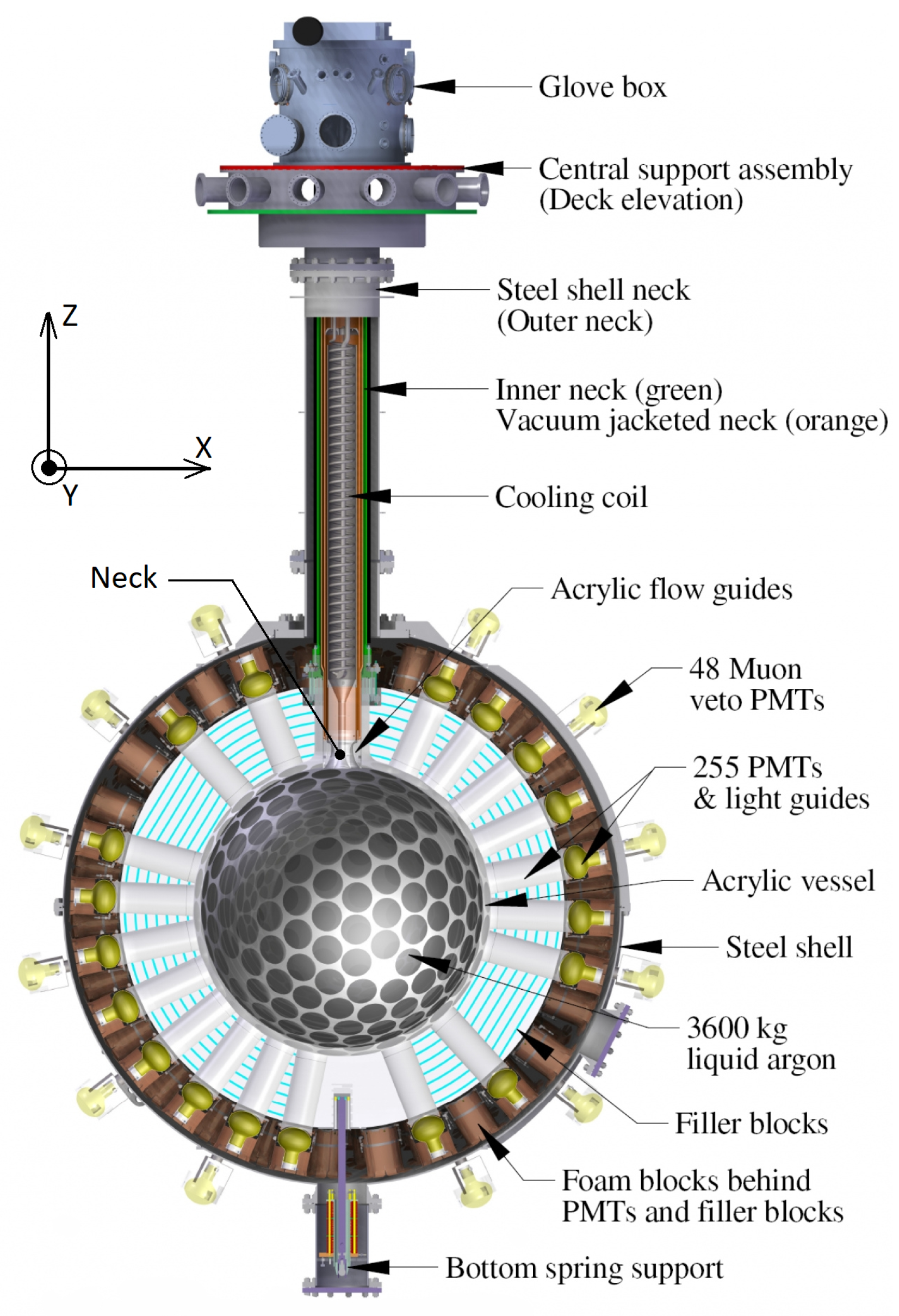
DEAP-3600 is a single-phase liquid argon detector located approximately 2 km (6 km water-equivalent) underground at the SNOLAB facility near Sudbury, Canada. The detector was built to register scintillation light induced by elastic scattering of WIMPs on nuclei of a 3279 kg liquid argon (LAr) target during the second fill, contained in a spherical acrylic vessel with an inner diameter of 1.7 m. The upper 30 cm of the acrylic vessel contains gaseous argon (GAr). The neck of the detector connects the acrylic vessel with the central support assembly, on which the glovebox is located (Figure 1).
The GAr and LAr regions are viewed by an array of 255 inward-facing 8 diameter photomultiplier tubes (PMTs) [4]. These PMTs are optically coupled to 45 cm long ultraviolet absorbing acrylic light guides, which transport visible photons from the acrylic vessel (AV) to the PMTs. The inner surface of the acrylic vessel is coated with a 3 μ m layer of 1,1,4,4-tetraphenyl-1,3-butadiene that converts 128 nm scintillation light produced by the LAr to visible wavelengths over a spectrum that peaks at 420 nm [5].
Figure 1. Schematic diagram of the DEAP-3600 detector [1]. The origin of the coordinate system is located at the center of the acrylic vessel, with the Z coordinate in the vertical direction.
Physics 05 00033 g001
The detector is well protected against particles from the outside. The space between the light guides is filled with alternating layers of high-density polyethylene and polystyrene foam filling blocks that provide passive protection of the detector components from neutrons. At the same time, the structure is enclosed in a spherical stainless steel shell and is submerged in a 7.8 m high, 7.8 m wide water tank with 48 outward facing 8″ diameter PMTs mounted on the outer surface of the sphere. Altogether, these photomultiplier tubes and the water tank constitute the Cherenkov muon veto used to mark the cosmogenic-induced background, while the shielding water provides neutron and gamma-ray background suppression from the cave [1].
The coordinate system is shown schematically in Figure 1. It originates from the center of the acrylic vessel. Thus, the X and Y coordinates lie within (−850; 850) mm, while in the Z axis, these limits are (−850; 1100) mm due to the presence of events in the detector neck.
The largest contribution to the background rate after applying fiducial cuts is from 210Po α -decays in the neck area of the detector. Scintillation light is observed resulting from neck events, which result from a thin film of LAr covering the surfaces of the neck components [1]. Such events are quite similar to events with nuclear recoil of the particle at the argon nucleus in the detector bulk, so backgrounds originating in the neck reduce the sensitivity of the detector. Proper recovery of the coordinates of events in the detector’s neck area will allow such events to be correctly identified and rejected in further analysis.
Two different position reconstruction algorithms developed by the DEAP-3600 collaboration are currently used. The first algorithm, called “MBLikelihood” (MBL), relies solely on the spatial distribution of charge through PMTs for position reconstruction. The second algorithm, called “TimeFit2” (TF2), uses the arrival time of the photons to determine the position of the event. Both methods use the maximum likelihood function in comparing the available information about the particle (charge, photoelectron arrival time) with the values in the grid of test positions inside the detector [1]. The likelihood functions in TF2 and MBL operate under the assumption that events originate in the LAr bulk—this causes a bias in the case of events originating from the neck. Therefore, both algorithms work well in the LAr area of the detector, but for events in the neck region, they do not match in their results and cannot accurately determine the event position.
To solve this, it was decided to use machine learning techniques to determine the position of the event in the entire detector volume, including the neck area.

3. Machine Learning Approach

Machine learning is widely used in elementary particle physics. Over the past two decades, particle physics has shifted to using machine learning methods to collect and analyze large samples of data [6]. Novel studies using neural networks [7,8] and boosted decision trees (BDTs) [9,10] in previous generation experiments [11,12,13,14,15,16,17,18,19,20,21,22] laid the foundation for the emergence of machine learning as an important tool at the LHC (Large Hadron Collider). Machine learning algorithms have made significant contributions to the discovery of the Higgs boson [23,24], and most data analysis tasks now benefit from machine learning. In parallel, the field of machine learning has evolved at a rapid pace, and in particular, the deep learning area has provided superior performance in several areas [25,26]. Incorporating these tools while maintaining the scientific rigor required to analyze elementary particle physics data broadens the horizons of science [27].
While investigating machine learning methods for position reconstruction in DEAP-3600, several methods were considered. Classical regression, support vectors, decision trees, dimensionality reduction using principal components, convolutional and fully connected neural networks are only a partial list of the algorithms that were tested for this problem. As a result, it is found that one of the most effective and fastest algorithms is the fully connected neural network (FCNN).

3.1. Neural Network Algorithm

The neural network [28] is a machine learning algorithm with: an input layer, in which the number of base units called “neurons” is equivalent to the number of event parameters; an output layer, in which the number of neurons corresponds to the number of variables being defined; and any number of “hidden” layers, in which there can be any number of neurons. A fully connected neural network is a neural network, in which each neuron of the layer is connected to all neurons of the next and previous layers. These connections are weight values and are adjusted during training. A schematic of the fully connected neural network is shown in Figure 2.
The principle of the neural network is as follows. There is a set of layers with a certain number of neurons in them. Each neuron has its activation function, which takes as its argument the weighted average of values from all neurons of the previous layer. In other words, each neuron receives all output values from previous layers, as well as weight values,
y i = F ( X ) = F w i a i ,
where F is the activation function of the neuron, w i is the weight of the connection which connects the current neuron with the ith neuron of the previous layer, and a i is the output value of the ith neuron of the previous layer. Model training consists of epochs, during which the training set is processed by the network. The training data are usually divided into batches, and after each batch is processed, the error is recalculated and the weights adjusted. The processing of one batch is called an iteration and consists of two parts. In the first part, a forward pass is performed from the beginning to the end, the error of the algorithm is calculated, and then a backward pass occurs, during which the weight values w i are adjusted in accordance with the measured error value. The main task of the neural network training is to determine these weight w i values.

3.2. Results

For the current study, using the ROOT [29], Geant4 [30] and RAT [31] software packages, sets of Monte Carlo simulations of three types of events of 50,000 each were created: β -decays of 39Ar, 40Ar nuclear recoil events, and α -decays of 210Po in the detector neck area.
In sum, 150,000 events were used in a 70:30 ratio to train and test the model. An equal number of events were performed to make sure that the algorithm was not overtrained on specific events.
Variables that were fed to the input layer of the neural network used 255 values of charge detected at the internal PMTs, normalized on a scale from zero to one.
The study was performed using the Python programming language [32]. During the analysis the following packages were used: pandas [33] and NumPy [34] for reading and converting data, and matplotlib [35] for graphics and TensorFlow [36] for building a machine learning model. A different neural network was trained for each of the three coordinates X, Y, Z. Due to the symmetry of the detector along the X and Y coordinates, the structure of the neural network for these coordinates is identical. Due to the fact that the detector symmetry is broken for the Z coordinate because of the presence of the detector neck, a model with a similar but slightly different structure was built for this coordinate. The structures of all three models were selected by an analytical method, however, adhering to the following rule: it is better to increase the number of neurons in the existing layers than to add a new layer. All models were compiled with the Adam optimizer [37] and mean squared error (MSE) loss metrics.
As a result, the following neural network structure was used for X and Y coordinates:
255 sigmoid 255 sigmoid 255 sigmoid 16 sigmoid 1 linear ,
and similar one for Z coordinate:
255 softmax 512 tan h 512 tan h 1 linear ,
where in numerator/denominator we have the number of neurons and the activation function on each layer, respectively.
Each model was trained to obtain a stable performance, and it was imperative they were not under-trained or over-trained. It turned out that 400 training epochs were sufficient for the first two models, while the last model for the Z coordinate became stable after 40 epochs. It also turned out that the models were optimal with batch sizes of 256 and 128 for X–Y and Z coordinates, respectively.
The models were tested after training. The test sample was divided into two parts: the first part contained events where the true position was in the LAr area of the detector, and the second part contained events that occurred in the detector neck area.
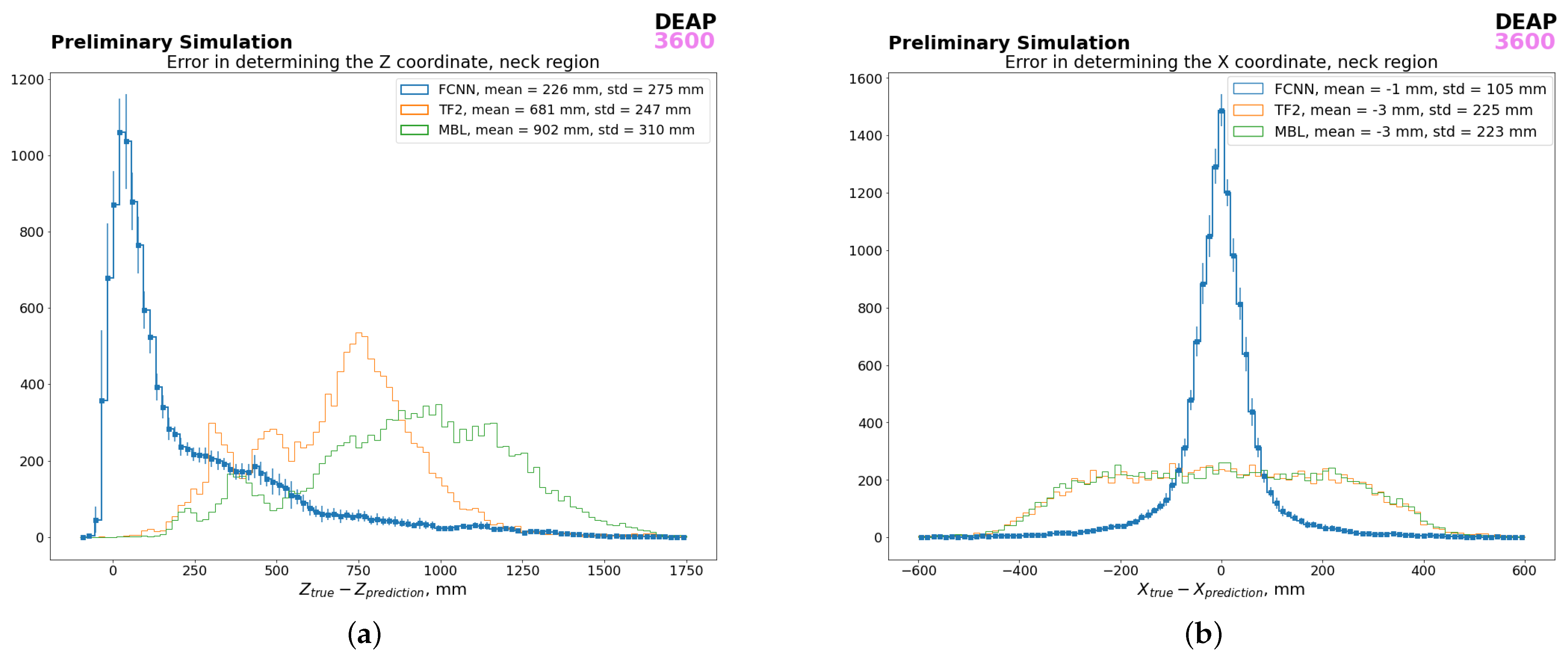
Figure 3 represents the main result of the study, and shows the graphs of the error in determining the coordinates (true minus reconstructed coordinates) for all three models: for the neural network (FCNN), TF2 and MBL.
Figure 3a shows the main result of this study. One can see that the neural network model works and reconstructs the Z coordinate more accurately than existing MBL and TF2 algorithms. Figure 3b shows that the neural network algorithm performs well also in determining the X coordinate in the neck region. Similar results are obtained for the Y coordinate.
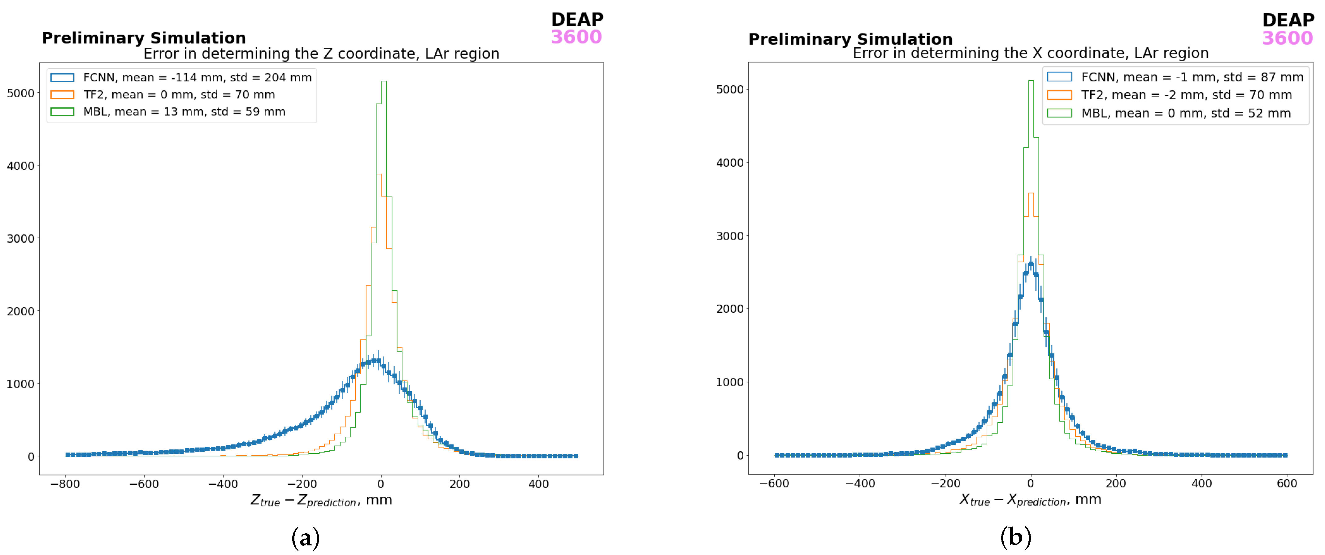
While the neural network-based algorithm performs well in the neck region (Figure 3), Figure 4 shows that this algorithm does not achieve the same results as the existing MBL algorithm in the LAr region. Nevertheless, the neural network results may also be taken into account as one of the three estimates of the event position for the most correct estimation of the weighted average.

4. Conclusions

This paper investigated a machine learning method for reconstructing the event position in the DEAP-3600 experiment. Multiple machine learning methods were researched, and the fully connected neural network has shown itself to be the most successful. A total of 150,000 simulated data events were generated by the Monte Carlo method for training and testing machine learning models. The trained models were tested on the test sample and these models were compared with the existing MBLikelihood and TimeFit2 algorithms. Based on the results of the test, it was determined that the model based on machine learning is best to reconstruct the events in the neck area of the detector (Figure 3). The machine learning neural network algorithm is found to also handle events in the LAr area while with a lower accuracy than that of the existing algorithms (Figure 4); however, it also contributes to the final position estimate. The machine learning algorithm method can be used separately to identify neck events as well as in combination with the already existing algorithms to get a more accurate assessment of the event position in the detector.

Funding

We thank the Natural Sciences and Engineering Research Council of Canada (NSERC), the Canada Foundation for Innovation (CFI), the Ontario Ministry of Research and Innovation (MRI), and Alberta Advanced Education and Technology (ASRIP), the University of Alberta, Carleton University, Queen’s University, the Canada First Research Excellence Fund through the Arthur B. McDonald Canadian Astroparticle Physics Research Institute, Consejo Nacional de Ciencia y Tecnología Project No. CONACYT CB-2017-2018/A1-S-8960, DGAPA UNAM Grants No. PAPIIT IN108020 and IN105923, and Fundación Marcos Moshinsky, the European Research Council Project (ERC StG 279980), the UK Science and Technology Facilities Council (STFC) (ST/K002570/1 and ST/R002908/1), the Leverhulme Trust (ECF-20130496), the Russian Science Foundation (Grant No. 21-72-10065), the Spanish Ministry of Science and Innovation (PID2019-109374GB-I00) and the Community of Madrid (2018-T2/ TIC-10494), the International Research Agenda Programme AstroCeNT (MAB/2018/7) funded by the Foundation for Polish Science (FNP) from the European Regional Development Fund, and the European Union’s Horizon 2020 research and innovation program under grant agreement No 952480 (DarkWave). Studentship support from the Rutherford Appleton Laboratory Particle Physics Division, STFC and SEPNet PhD is acknowledged.

Data Availability Statement

Not applicable.

Acknowledgments

We thank SNOLAB and its staff for support through underground space, logistical, and technical services. SNOLAB operations are supported by the CFI and Province of Ontario MRI, with underground access provided by Vale at the Creighton mine site. We thank Vale for their continuing support, including the work of shipping the acrylic vessel underground. We gratefully acknowledge the support of the Digital Research Alliance of Canada, Calcul Québec, the Centre for Advanced Computing at Queen’s University, and the Computational Centre for Particle and Astrophysics (C2PAP) at the Leibniz Supercomputer Centre (LRZ) for providing the computing resources required to undertake this work.

Conflicts of Interest

The authors declare no conflict of interest.

Appendix A. Membership of the DEAP Collaboration

P. Adhikari 6 , R. Ajaj 6 , 28 , M. Alpízar-Venegas 15 , P.-A. Amaudruz 26 , J. Anstey 6 , 28 , D. J. Auty 1 , M. Baldwin 23 , M. Batygov 13 , B. Beltran 1 , C. E. Bina 1 , 28 , W. Bonivento 10 , M. G. Boulay 6 , J. F. Bueno 1 , P. M. Burghardt 27 , A. Butcher 22 , M. Cadeddu 10 , B. Cai 6 , 28 , M. Cárdenas-Montes 7 , S. Cavuoti 9 , 12 , Y. Chen 1 , S. Choudhary 2 , B. T. Cleveland 24 , 13 , R. Crampton 6 , 28 , S. Daugherty 24 , 13 , 6 , P. DelGobbo 6 , 28 , P. Di Stefano 21 , G. Dolganov 17 , L. Doria 20 , F. A. Duncan 24 , a , M. Dunford 6 , 28 , E. Ellingwood 21 , A. Erlandson 6 , 4 , S. S. Farahani 1 , N. Fatemighomi 24 , 22 , G. Fiorillo 8 , 12 , R. J. Ford 24 , 13 , D. Gallacher 6 , P. García Abia 7 , S. Garg 6 , P. Giampa 21 , 26 , b , A. Giménez-Alcázar 7 , D. Goeldi 6 , 28 , P. Gorel 24 , 13 , 28 , K. Graham 6 , A. Grobov 17 , A. L. Hallin 1 , M. Hamstra 6 , 21 , S. Haskins 6 , 28 , J. Hu 1 , J. Hucker 21 , T. Hugues 2 , A. Ilyasov 17 , 18 , * , B. Jigmeddorj 24 , 13 , C. J. Jillings 24 , 13 , A. Joy 1 , 28 , G. Kaur 6 , A. Kemp 22 , 21 , M. Kuźniak 2 , 6 , 28 , F. La Zia 22 , M. Lai 3 , 10 , S. Langrock 13 , 28 , B. Lehnert 14 , J. LePage-Bourbonnais 6 , 28 , N. Levashko 17 , 18 , M. Lissia 10 , I. Machulin 17 , 18 , P. Majewski 23 , A. Maru 6 , 28 , J. Mason 6 , 28 , A. B. McDonald 21 , T. McElroy 1 , J. B. McLaughlin 22 , 26 , C. Mielnichuk 1 , L. Mirasola 3 , 10 , J. Monroe 22 , C. Ng 1 , G. Oliviéro 6 , 28 , S. Pal 1 , 28 , D. Papi 1 , S. J. M. Peeters 25 , M. Perry 6 , V. Pesudo 7 , E. Picciau 10 , 3 , T. R. Pollmann 27 , 13 , 21 , c , F. Rad 6 , 28 , C. Rethmeier 6 , F. Retière 26 , I. Rodríguez García 7 , L. Roszkowski 2 , 16 , R. Santorelli 7 , F. G. Schuckman II 21 , N. Seeburn 22 , S. Seth 6 , 28 , V. Shalamova 5 , P. Skensved 21 , N. J. T. Smith 24 , 13 , K. Sobotkiewich 6 , T. Sonley 24 , 6 , 28 , J. Sosiak 6 , 28 , J. Soukup 1 , R. Stainforth 6 , M. Stringer 21 , 28 , J. Tang 1 , E. Vázquez-Jáuregui 15 , S. Viel 6 , 28 , B. Vyas 6 , M. Walczak 2 , J. Walding 22 , M. Ward 21 , S. Westerdale 5 , J. Willis 1 , A. Zuñiga-Reyes 15

Affiliations

1
Department of Physics, University of Alberta, Edmonton, Alberta, T6G 2R3, Canada
2
AstroCeNT, Nicolaus Copernicus Astronomical Center, Polish Academy of Sciences, Rektorska 4, 00-614 Warsaw, Poland
3
Physics Department, Università degli Studi di Cagliari, Cagliari 09042, Italy
4
Canadian Nuclear Laboratories, Chalk River, Ontario, K0J 1J0, Canada
5
Department of Physics and Astronomy, University of California, Riverside, CA 92507, USA
6
Department of Physics, Carleton University, Ottawa, Ontario, K1S 5B6, Canada
7
Centro de Investigaciones Energéticas, Medioambientales y Tecnológicas, Madrid 28040, Spain
8
Physics Department, Università degli Studi “Federico II” di Napoli, Napoli 80126, Italy
9
Astronomical Observatory of Capodimonte, Salita Moiariello 16, I-80131 Napoli, Italy
10
INFN Cagliari, Cagliari 09042, Italy
11
INFN Laboratori Nazionali del Gran Sasso, Assergi (AQ) 67100, Italy
12
INFN Napoli, Napoli 80126, Italy
13
School of Natural Sciences, Laurentian University, Sudbury, Ontario, P3E 2C6, Canada
14
Nuclear Science Division, Lawrence Berkeley National Laboratory, Berkeley, CA 94720, USA
15
Instituto de Física, Universidad Nacional Autónoma de México, A.P. 20-364, Ciudad de México D. F. 01000, Mexico
16
BP2, National Centre for Nuclear Research, ul. Pasteura 7, 02-093 Warsaw, Poland
17
National Research Centre Kurchatov Institute, Moscow 123182, Russia
18
National Research Nuclear University MEPhI, Moscow 115409, Russia
19
Physics Department, Princeton University, Princeton, NJ 08544, USA
20
PRISMA+ Cluster of Excellence and Institut für Kernphysik, Johannes Gutenberg-Universität Mainz, 55128 Mainz, Germany
21
Department of Physics, Engineering Physics, and Astronomy, Queen’s University, Kingston, Ontario, K7L 3N6, Canada
22
Royal Holloway University London, Egham Hill, Egham, Surrey TW20 0EX, United Kingdom
23
Rutherford Appleton Laboratory, Harwell Oxford, Didcot OX11 0QX, United Kingdom
24
SNOLAB, Lively, Ontario, P3Y 1M3, Canada
25
University of Sussex, Sussex House, Brighton, East Sussex BN1 9RH, United Kingdom
26
TRIUMF, Vancouver, British Columbia, V6T 2A3, Canada
27
Department of Physics, Technische Universität München, 80333 Munich, Germany
28
Arthur B. McDonald Canadian Astroparticle Physics Research Institute, Queen’s University, Kingston, ON, K7L 3N6, Canada
a
Deceased
b
Currently at SNOLAB, Lively, Ontario, P3Y 1M3, Canada
c
Currently at Nikhef and the University of Amsterdam, Science Park, 1098XG Amsterdam, Netherlands
*
Correspondence: [email protected]

References

  1. Ajaj, R. et al. [DEAP Collaboration] Search for dark matter with a 231-day exposure of liquid argon using DEAP-3600 at SNOLAB. Phys. Rev. D 2019, 100, 022004. [Google Scholar] [CrossRef]
  2. Aghanim, N. et al. [Planck Collaboration] Planck 2018 results. VI. Cosmological parameters. Astron. Astrophys. 2020, 641, A6. [Google Scholar]
  3. Amaudruz, P.A. et al. [DEAP Collaboration] Design and construction of the DEAP-3600 dark matter detector. Astropart. Phys. 2019, 108, 1–23. [Google Scholar] [CrossRef]
  4. Amaudruz, P.A. et al. [DEAP Collaboration] In-Situ characterization of the Hamamatsu R5912-HQE photomultiplier tubes used in the DEAP-3600 experiment. Nucl. Instrum. Meth. Phys. Res. A 2019, 922, 373–384. [Google Scholar] [CrossRef]
  5. Francini, R.; Montereali, R.M.; Nichelatti, E.; Vincenti, M.A.; Canci, N.; Segreto, E.; Cavanna, F.; Di Pompeo, F.; Carbonara, F.; Fiorillo, G.; et al. Tetraphenyl-butadiene films: VUV-Vis optical characterization from room to liquid argon temperature. J. Instrum. 2013, 8, C09010. [Google Scholar] [CrossRef]
  6. Bhat, P.C. Multivariate analysis methods in particle physics. Annu. Rev. Nucl. Part. Sci. 2011, 61, 281–309. [Google Scholar] [CrossRef]
  7. Rosenblatt, F. Principles of Neurodynamics. Perceptrons and the Theory of Brain Mechanisms; Report No. VG-II96-G-8; Cornell Aeronautical Laboratory, Inc.; Cornell University: Buffalo, NY, USA, 1961; Available online: https://apps.dtic.mil/sti/citations/AD0256582 (accessed on 1 April 2023).
  8. Reed, R.D.; Marks, R.J., II. Neural Smithing: Supervised Learning in Feedforward Artificial Neural Networks; The MIT Press: Cambridge, MA, USA, 1999. [Google Scholar]
  9. Breiman, L.; Friedman, J.; Stone, C.J.; Olshen, R.A. Classification and Regression Trees; Chapman & Hall; CRC; Taylor & Francis Group, LLC: Boca Raton, FL, USA, 1984. [Google Scholar] [CrossRef]
  10. Freund, Y.; Schapire, R.E. A decision-theoretic generalization of on-line learning and an application to boosting. J. Comput. Syst. Sci. 1997, 55, 119–139. [Google Scholar] [CrossRef]
  11. Peterson, C.; Rögnvaldsson, T. An introduction to artificial neural networks. In 1991 CERN School of Computing; Verkerk, C., Ed.; CERN: Geneva, Switzerland, 1992; pp. 113–170. [Google Scholar] [CrossRef]
  12. Barate, R. et al. [The ALEPH Collaboration] Determination of |Vub| from the measurement of the inclusive charmless semileptonic branching ratio of b hadrons. Eur. Phys. J. C 1999, 6, 555–574. [Google Scholar] [CrossRef]
  13. Akers, R. et al. [OPAL Collaboration] A measurement of the production of D*± mesons on the Z0 resonance. Z. Phys. C 1995, 67, 27–44. [Google Scholar] [CrossRef]
  14. Chiappetta, P.; Colangelo, P.; De Felice, P.; Nardulli, G.; Pasquariello, G. Higgs search by neural networks at LHC. Phys. Lett. B 1994, 322, 219–223. [Google Scholar] [CrossRef]
  15. Peterson, C.; Rögnvaldsson, T.; Lönnblad, L. JETNET 3.0—A versatile artificial neural network package. Comput. Phys. Commun. 1994, 81, 185–220. [Google Scholar] [CrossRef]
  16. Buskulic, D. et al. [ALEPH Collaboration] Measurement of the tau polarisation at the Z resonance. Z. Phys. C 1993, 59, 369–386. [Google Scholar] [CrossRef]
  17. Babbage, W.S.; Thompson, L.F. The use of neural networks in γ-π0 discrimination. Nucl. Instrum. Meth. Phys. Res. A 1993, 330, 482–486. [Google Scholar] [CrossRef]
  18. Lönnblad, L.; Peterson, C.; Rögnvalsson, T. Pattern recognition in high energy physics with artificial neural networks—JETNET 2.0. Comput. Phys. Commun. 1992, 70, 167–182. [Google Scholar] [CrossRef]
  19. Lönnblad, L.; Peterson, C.; Rögnvaldsson, T. Using neural networks to identify jets. Nucl. Phys. B 1991, 349, 675–702. [Google Scholar] [CrossRef]
  20. Lönnblad, L.; Peterson, C.; Rögnvaldsson, T. Finding gluon jets with a neural trigger. Phys. Rev. Lett. 1990, 65, 1321. [Google Scholar] [CrossRef]
  21. Denby, B. Neural networks and cellular automata in experimental high energy physics. Comput. Phys. Commun. 1988, 49, 429–448. [Google Scholar] [CrossRef]
  22. Roe, B.P.; Yang, H.J.; Zhu, J.; Liu, Y.; Stancu, I.; McGregor, G. Boosted decision trees as an alternative to artificial neural networks for particle identification. Nucl. Instrum. Meth. Phys. Res. A 2005, 543, 577–584. [Google Scholar] [CrossRef]
  23. Aad, G. et al. [ATLAS Collaboration] Observation of a new particle in the search for the Standard Model Higgs boson with the ATLAS detector at the LHC. Phys. Lett. B 2012, 716, 1–29. [Google Scholar] [CrossRef]
  24. Chatrchyan, S. et al. [CMS Collaboration] Observation of a new boson at a mass of 125 GeV with the CMS experiment at the LHC. Phys. Lett. B 2012, 716, 30–61. [Google Scholar] [CrossRef]
  25. Silver, D.; Huang, A.; Maddison, C.J.; Guez, A.; Sifre, L.; van den Driessche, G.; Schrittwieser, J.; Antonoglou, I.; Panneershelvam, V.; Lanctot, M.; et al. Mastering the game of Go with deep neural networks and tree search. Nature 2016, 529, 484–489. [Google Scholar] [CrossRef] [PubMed]
  26. Russakovsky, O.; Deng, J.; Su, H.; Krause, J.; Satheesh, S.; Ma, S.; Huang, Z.; Karpathy, A.; Khosla, A.; Bernstein, M.; et al. ImageNet Large Scale Visual Recognition Challenge. Int. J. Comput. Vis. 2015, 115, 211–252. [Google Scholar] [CrossRef]
  27. Radovic, A.; Williams, M.; Rousseau, D.; Kagan, M.; Bonacorsi, D.; Himmel, A.; Aurisano, A.; Terao, K.; Wongjirad, T. Machine learning at the energy and intensity frontiers of particle physics. Nature 2018, 560, 41–48. [Google Scholar] [CrossRef]
  28. Hopfield, J.J. Neural networks and physical systems with emergent collective computational abilities. Proc. Natl. Acad. Sci. USA 1982, 79, 2554–2558. [Google Scholar] [CrossRef]
  29. Brun, R.; Rademakers, F. ROOT: An object oriented data analysis framework. Nucl. Instrum. Meth. Phys. Res. A 1997, 389, 81–86. [Google Scholar] [CrossRef]
  30. Agostinelli, S.; Allison, J.; Amako, K.; Apostolakis, J.; Araujo, H.; Arce, P.; Asai, M.; Axen, D.; Banerjee, S.; Barrand, G.; et al. GEANT4—A simulation toolkit. Nucl. Instrum. Meth. Phys. Res. A 2003, 506, 250–303. [Google Scholar] [CrossRef]
  31. Bolton, T.; Gastler, D.; Klein, J.; Lippincott, H.; Mastbaum, A.; Nikkel, J.; Orebi Gann, G.; Akashi-Ronquest, M.; Seibert, S.; Sekula, S.; et al. RAT (Is an Analysis Tool) User’s Guide. 2018. Available online: https://rat.readthedocs.io/ (accessed on 1 April 2023).
  32. Van Rossum, G.; Drake, F.L. Python 3 Reference Manual; CreateSpace: Scotts Valley, CA, USA, 2009. [Google Scholar]
  33. McKinney, W. Data structures for statistical computing in Python. In Proceedings of the 9th Python in Science Conference (SciPy 2010), Austin, TX, USA, 28 – 30 June 2010; pp. 56–61. [Google Scholar] [CrossRef]
  34. Harris, C.R.; Millman, K.J.; van der Walt, S.J.; Gommers, R.; Virtanen, P.; Cournapeau, D.; Wieser, E.; Taylor, J.; Berg, S.; Smith, N.J.; et al. Array programming with NumPy. Nature 2020, 585, 357–362. [Google Scholar] [CrossRef]
  35. Hunter, J.D. Matplotlib: A 2D graphics environment. Comput. Sci. Eng. 2007, 9, 90–95. [Google Scholar] [CrossRef]
  36. Abadi, M.; Agarwal, A.; Barham, P.; Brevdo, E.; Chen, Z.; Citro, C.; Corrado, G.S.; Davis, A.; Dean, J.; Devin, M.; et al. TensorFlow: Large-scale machine learning on heterogeneous systems. arXiv 2016, arXiv:1603.04467. [Google Scholar] [CrossRef]
  37. Kingma, D.P.; Ba, J. Adam: A method for stochastic optimization. arXiv 2014, arXiv:1412.6980. [Google Scholar] [CrossRef]
Figure 2. Schematic and operating principle of a fully connected neural network. a i is the output value of the ith neuron of the previous layer. “PMT” stands for the “photomultiplier”.
Physics 05 00033 g002
Figure 3. Error in determining the Z (a) and X (b) coordinates in the detector neck area. Results of different algorithms are shown: the fully connected neural network (“FCNN”), TimeFit2 (“TF2”), and MBLikehood (“MBL”); see text for details. The “std” stands for the standard deviation.
Physics 05 00033 g003
Figure 4. Error in determining the Z (a) and X (b) coordinates in the detector LAr area. Results of different algorithms are shown: the fully connected neural network (“FCNN”), TimeFit2 (“TF2”), and MBLikehood (“MBL”); see text for details. The “std” stands for the standard deviation.
Physics 05 00033 g004
Disclaimer/Publisher’s Note: The statements, opinions and data contained in all publications are solely those of the individual author(s) and contributor(s) and not of MDPI and/or the editor(s). MDPI and/or the editor(s) disclaim responsibility for any injury to people or property resulting from any ideas, methods, instructions or products referred to in the content.