Finite-Series Approximation of the Bound States for Two Novel Potentials

Abstract

We obtain an analytic approximation of the bound states solution of the Schrödinger equation on the semi-infinite real line for two potential models with a rich structure as shown by their spectral phase diagrams. These potentials do not belong to the class of exactly solvable problems. The solutions are finite series (with a small number of terms) of square integrable functions written in terms of Romanovski–Jacobi polynomials.

1. Introduction

Fundamental interactions in nature are very few. In fact, of those interactions only four known that may even be unified (merged) into fewer interactions as the energy scale becomes very large. In quantum mechanics, these fundamental interactions are modelled (in simple systems) by even fewer potential functions (e.g., $r^{-1}$ for the Coulomb and Kepler problems, $r^2$ for quarks interaction, etc., where r is the radial coordinate). However, for complex systems (e.g., those with a large number of constituents), the fundamental interactions become intractable and modelling using simple potential functions becomes non-trivial to almost impossible. However, potential models formed using various functions that satisfy basic physical constraints can give a good description of certain aspects of the system. For example, the binding of some molecules can be described extremely accurately by the Morse potential with a proper choice of parameters. Consequently, the search for potential functions that can model the structure and dynamics of various physical systems started at the early conception of quantum mechanics and still continues. Of all these models, the most interesting are those that can be solved exactly for the whole energy spectrum or for a finite portion thereof. The latter solution is referred to as “quasi-exact”. Nonetheless, the number of such potential functions is very small. Physicists continue to develop methods to enlarge the class of exactly solvable potential models. Meanwhile, approximate solutions of the wave equation (relativistic and non-relativistic) with interesting potential models dominate the literature. Most of these approximations are numerical in nature. The most important requirement of such models is that the corresponding potential functions must have a rich structure with a sufficient (but not large) number of parameters that could be tuned to fit experimental measurements of the target system being modelled. The two main features of the study here are:

(1)

The two potential models which are considered have rich structures, as evidenced by their spectral phase diagrams and each having four tunable parameters.

(2)

The approximate solutions obtained are analytic and written as finite series with a small number of terms involving mathematically well-defined objects.

In this study, we use the tridiagonal representation approach (TRA) [1] to obtain approximations of bound state solutions of the Schrödinger equation for the following four-parameter potential models:

$$V_{\mathrm{I}}(x)=\frac{2}{x^2+2a^2}\left[\frac{a^{2}A}{x^2}-\frac{a^{2}B}{x^2+2a^2}+C\right]=\frac{A}{x^2}+\frac{2C-A}{x^2+2a^2}-\frac{2a^{2}B}{{\left(x^2+2a^2\right)}^2},$$

(1a)

$$V_{\mathrm{II}}(x)=\frac{1}{x\left(x+2a\right)}\left[\frac{a^{2}A}{x\left(x+2a\right)}-\frac{a^{2}B}{{\left(x+a\right)}^2}+C\right]=\frac{A/4}{x^2}+\frac{2C-2B-A}{2x\left(x+2a\right)}+\frac{A/4}{{\left(x+2a\right)}^2}+\frac{B}{{\left(x+a\right)}^2},$$

(1b)

where $x\ge 0$ denotes the space coordinate and the scale parameter a is a positive dimension of length. The dimensionless real parameters $\left\{A,B,C\right\}$ are positive. The solutions are written as finite series of square integrable functions that carry a tridiagonal matrix representation for the wave operator. The potential functions (1a) and (1b) do not belong to the class of exactly solvable problems. Nonetheless, potential $V_{\mathrm{I}}(x)$ was treated in Section III.A.6 of Ref. [2] and in Section 2.4 of Ref. [3]. However, no exact TRA solutions were obtained because the matrix representation of the wave operator chosen therein was not tridiagonal, despite the fact that the Hamiltonian matrix is tridiagonal. Potential $V_{\mathrm{I}}(x)$ is an inverse square singular potential at the origin with a singularity strength, A. On the other hand, $V_{\mathrm{II}}(x)$ has an inverse square as well as an inverse linear singularity at the origin with respective strengths of $A/4$ and $(2C-2B-A)/4a$. Moreover, both potentials vanish at infinity. The upper limit on the number of bound states is obtained by evaluating the integral ${\displaystyle {\int }_0^{\infty }x{V}^{-}(x)dx}$, where $V^{-}(x)=-V(x)\theta \left[-V(x)\right]$ and $\theta (x)$ is the step function [4,5]. For $C>0$, the limits of integration 0 and $\infty$ become $x_{\pm }$, which are finite, and the value of the integral is also finite. However, for $C<0$, the upper limit $x_{+}$ is infinite and the integral diverges. Consequently, with $C>0$, the two potentials could support a mix of a finite number of bound states and resonances, whereas if $C<0$, the potentials could support an infinite number of bound states without resonances. The proper values of the potential parameters for supporting such structures must produce one or two positive real roots for the cubic equation that results from the condition ${\left(dV/dx\right)}_{x_0}=0$ with $x_0>0$. A necessary (but perhaps not sufficient) condition for the existence of bound states is $V(x_0)<0$. The existence of two different real positive roots of the cubic equation implies the possibility of resonances. The cubic equations associated with $V_{\mathrm{I}}(x)$ and $V_{\mathrm{II}}(x)$ are:

$$C{s}^3+2\left(C-B+A\right)s^2+6As+4A=0,$$

(2a)

$$C{t}^3+2\left(C-B+A\right)t^2+\left(C-B+4A\right)t+2A=0,$$

(2b)

respectively, where $s={\left(x/a\right)}^2$ and $t={(x/a)}^2+2(x/a)$. Since A and C are positive, Descartes’ rule of signs [6] for Equations (2a,b) dictates that B must be greater than $A+C$ resulting in two positive real roots. Thus, the spectrum will then consist of a mixture of a finite number of bound states and resonances. On the other hand, if C were negative, Descartes’ rule of signs would have implied a single positive real root for Equations (2a,b), resulting in an infinite number of pure bound states (without resonances). 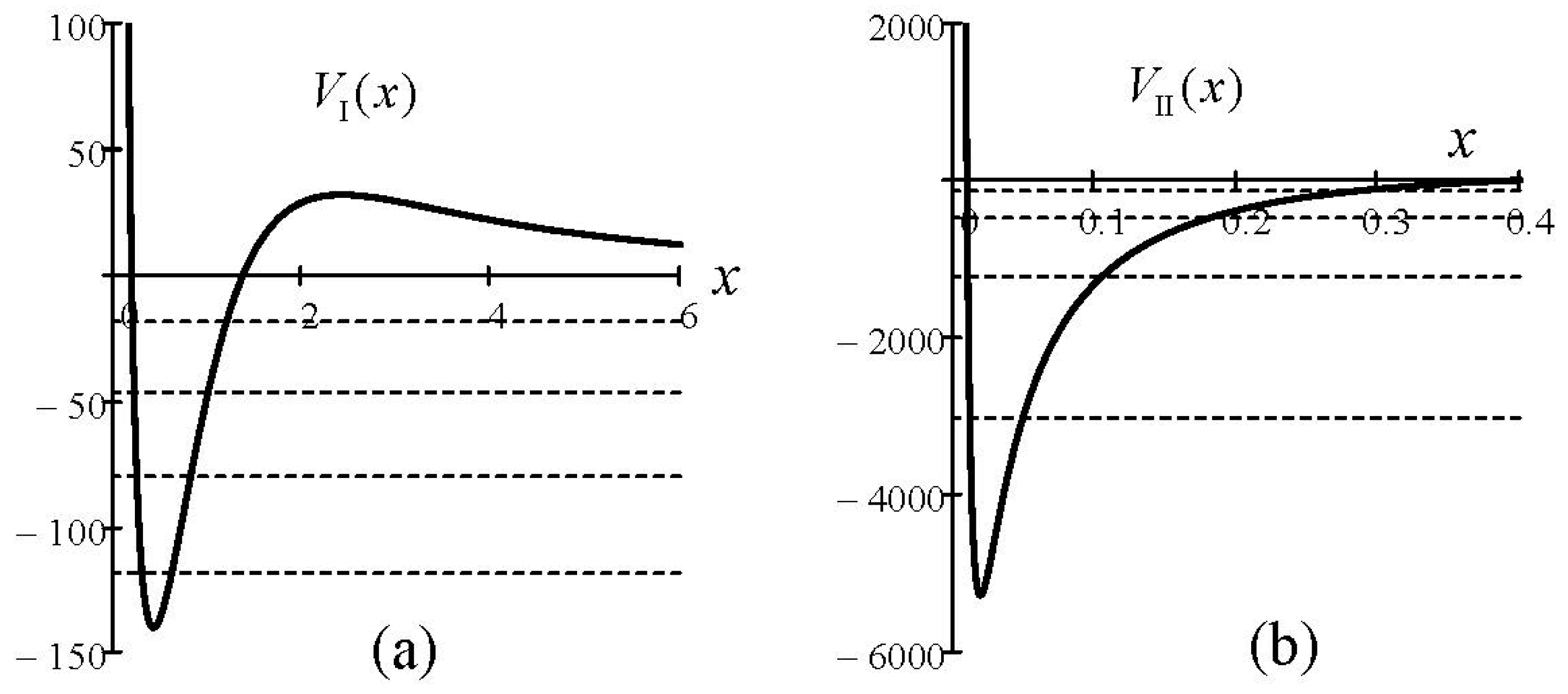Figure 1 shows several plots of the two potential functions (in units of $A/a^2$) for a fixed value of the parameter ratio $C/A$ and for different values of $B/A$. 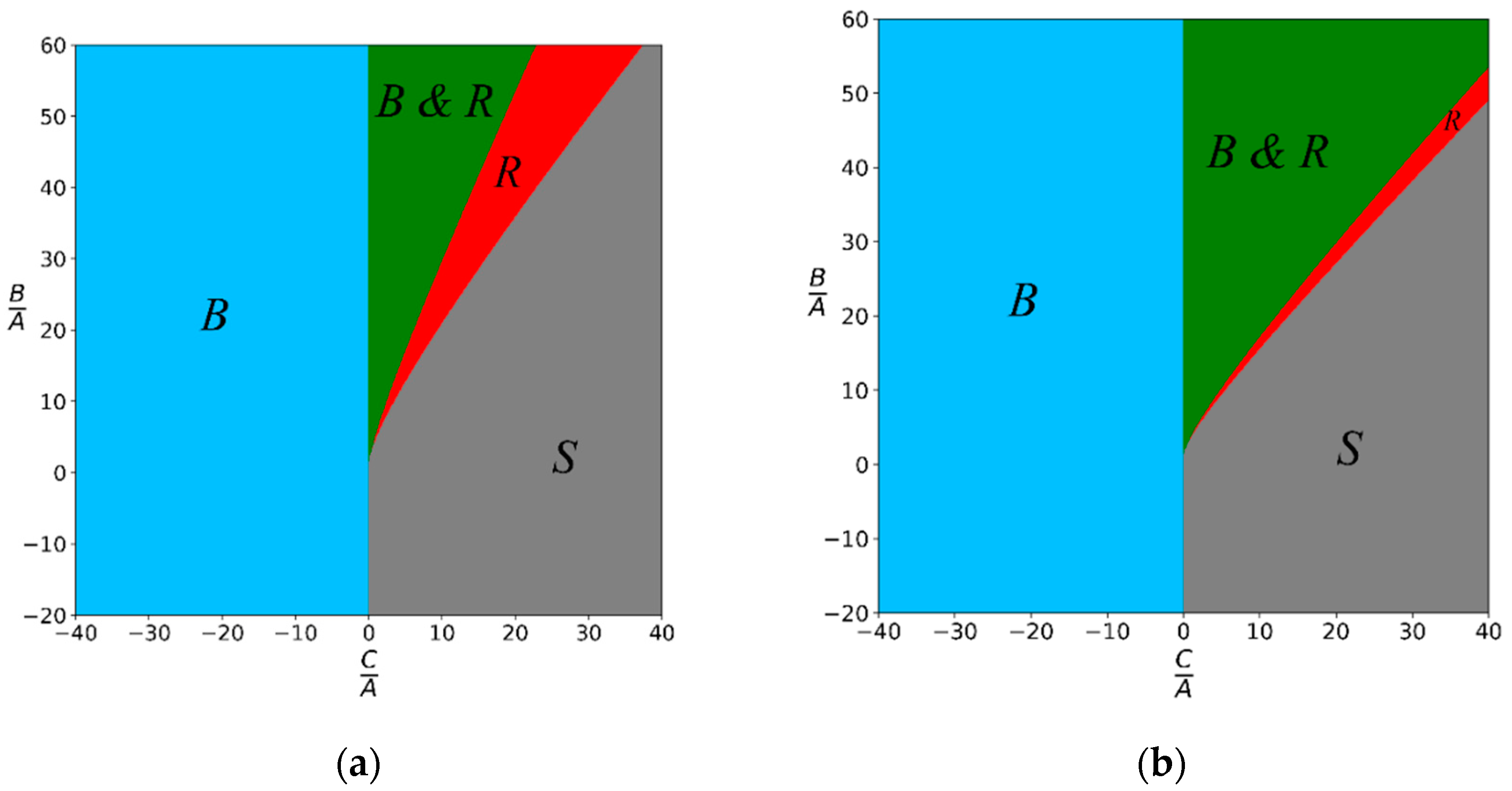Figure 2 presents a spectral phase diagram (SPD) of the two potentials, showing the distribution of their corresponding energy spectrum (scattering states, bound states, and resonances) as a function of the potential parameters. It should be noted that the observations made above about the sign of the potential parameter C are consistent with the SPDs shown in the figure. A detailed description of the SPD, its benefits, and how to construct it are found in Ref. [7].

In the atomic units $\hslash =m=1$, where h is the Planck’s constant and m is the mass, the time-independent Schrödinger equation in the configuration space x for the potential $V(x)$ and energy E is as follows:

$$\left[-\frac{1}{2}\frac{d^2}{d{x}^2}+V(x)-E\right]\psi (x)=0.$$

(3)

In the TRA [1,2], the solution of this equation, which we write as $\mathcal{D}\psi (x)=0$, where $\mathcal{D}$ is the wave operator, is written as a bounded convergent series of discrete square-integrable functions $\left\{{\varphi }_n\right\}$. That is, $\psi (x)={\displaystyle {\sum }_n{f}_n{\varphi }_n(y)}$, where $y=y(x)$ is a coordinate transformation and $\left\{f_n\right\}$ are the expansion coefficients. The basis set $\left\{{\varphi }_n\right\}$ must be complete and should result in a tridiagonal matrix representation for the wave operator, $\langle {\varphi }_n|\mathcal{D}|{\varphi }_m\rangle$, that is, the action of the wave operator on the basis element should read [1]:

$$\mathcal{D}{\varphi }_n(y)=W(y)\left[d_n{\varphi }_n(y)+c_{n-1}{\varphi }_{n-1}(y)+b_n{\varphi }_{n+1}(y)\right],$$

(4)

where W(y) is a nodeless entire function and $\left\{b_n,c_n,d_n\right\}$ are constant coefficients. Moreover, the integral ${\displaystyle {\int }_{x_{-}}^{x_{+}}{\varphi }_m(y)W(y){\varphi }_n(y)dx}$ must be proportional to ${\delta }_{m,n}$, where ${\delta }_{m,n}$ is the Kronecker delta. Hence, the wave equation $\mathcal{D}\psi (x)=0$ becomes a three-term recursion relation for the expansion coefficients $\left\{f_n\right\}$ as follows:

$$d_n{F}_n+b_{n-1}{F}_{n-1}+c_n{F}_{n+1}=0,$$

(5)

where we have written $f_n=f_0{F}_n$, making $F_0=1$. Accordingly, the solution of the wave equation, $\mathcal{D}\psi (x)=0$, reduces to an algebraic solution of the discrete Equation (5). Moreover, the set $\left\{f_n\right\}$ contains all physical information about the system modelled by the potential. It should be noted that, in general, the discrete sequence $\left\{F_n\right\}$ satisfying the three-term recursion relation (5) is an infinite sequence. Moreover, if $b_n{c}_n>0$ for all n, then ${\left\{F_n\right\}}_{n=0}^{\infty }$ is an orthogonal infinite sequence, that is, ${\displaystyle {\int }_{z_{-}}^{z_{+}}\omega (z)F_n(z)F_m(z)dz}\propto {\delta }_{n,m}$, where $\omega (z)$ is a positive weight function. However, as shown in Section 2 and Section 3 below, for the problem under consideration here, $b_n{c}_n>0$ only for $n\le N$. Therefore, only the subsequence ${\left\{F_n\right\}}_{n=0}^N$ forms an orthogonal set on the real line and thus we look for solutions of the wave equation $\mathcal{D}\psi (x)=0$ in the form of a finite series $\psi (x)=$ $f_0(z){\displaystyle {\sum }_{n=0}^N{F}_n(z){\varphi }_n(y)}$.

To solve for the continuous spectrum or for an infinite discrete spectrum of a given physical system, completeness of the set $\left\{{\varphi }_n\right\}$ implies that it is an infinite and dense set. However, for systems with a finite number of bound states, a finite basis set ${\left\{{\varphi }_n\right\}}_{n=0}^N$ could, actually, produce a physically faithful representation of the system, provided that the number of bound states is less than or equal to the size of the basis $N+1$. Additionally, for a quasi-exact solution where one looks for a finite portion of the infinite discrete spectrum, such a finite basis set could lead to a good approximation of that portion of the spectrum with an accuracy that increases as N does.

For the finite number of bound states of the system modelled by either $V_{\mathrm{I}}(x)$ or $V_{\mathrm{II}}(x)$, we choose a finite basis set with the following elements:

$${\varphi }_n(y)={(y-1)}^{\alpha }{(y+1)}^{-\beta }{J}_n^{(\mu ,\nu )}(y),$$

(6)

where $J_n^{(\mu ,\nu )}(y)$ is the Romanovski–Jacobi (R-Jacobi) polynomial, defined on the semi-infinite real line $y(x)\ge 1$, as shown in Appendix A. The real basis parameters $\left\{\alpha ,\beta ,\mu ,\nu \right\}$ are to be determined below in terms of the physical parameters $\left\{a,A,B,C\right\}$ by the TRA constraints. Moreover, $n=0,1,..,N$ with $N=\lfloor -\frac{\mu +\nu +1}{2}\rfloor$, where $\lfloor z\rfloor$ stands for the largest integer less than z. Therefore, the basis set, whose elements are given by Equation (6), is finite with a size equal to $N+1$.

In Section 2 and Section 3, we use the TRA to solve this equation for the two potential models. We conclude in Section 4 with some remarks and discussion of our findings.

2. TRA Solution of the Potential Model (1a)

In this case, we choose the coordinate transformation $y(x)={\left(x/a\right)}^2+1$. Writing the differential operator $\frac{d^2}{d{x}^2}$ and the potential $V_{\mathrm{I}}(x)$ in terms of the dimensionless variable y, Equation (4) becomes:

$$\mathcal{D}\psi (x)=-\frac{2/a^2}{y+1}\left[\left(y^2-1\right)\frac{d^2}{d{y}^2}+\frac{y+1}{2}\frac{d}{dy}-\frac{A}{y-1}+\frac{B}{y+1}-C+\frac{\epsilon }{2}\left(y+1\right)\right]\psi (x)=0,$$

(7)

where $\epsilon =a^{2}E$. This equation is the confluent Heun equation (see, for example, Equation (1.1.4) on p. 90 of Heun’s Differential Equations [8]). The solutions of this equation as an infinite expansion in terms of hypergeometric polynomials (Jacobi polynomials) are described in Section 2.3 of [8]. Here, we use a similar treatment but within the framework of the TRA and with finite expansion. Therefore, we write the solution as the series $\psi (x)={\displaystyle {\sum }_n{f}_n{\varphi }_n(y)}$. Consequently, we need to evaluate the action of the wave operator on the basis elements $\mathcal{D}|{\varphi }_n\rangle$ and then impose the TRA constraint (5). To achieve this, we choose the basis parameters $2\alpha =\mu +\frac{1}{2}$ and $2\beta =-\nu -1$, then use the differential equation of the R-Jacobi polynomial,$J_n^{(\mu ,\nu )}(y)$, given in Appendix A by Equation (A1), to obtain:

$$\begin{array}{c}\mathcal{D}|{\varphi }_n(y)\rangle =-\frac{1}{a^2}\frac{{(y-1)}^{\alpha }}{{(y+1)}^{\beta +1}}\{\frac{{\mu }^2-\frac{1}{4}}{y-1}-\frac{{\nu }^2-1}{y+1}+\frac{1}{2}\left[{\left(2n+\mu +\nu +1\right)}^2-\frac{1}{4}\right]\\ -\frac{2A}{y-1}+\frac{2B}{y+1}-2C+\epsilon \left(y+1\right)\}{J}_n^{(\mu ,\nu )}(y)\end{array}$$

(8)

The TRA constraint (5) and the recursion relation of the R-Jacobi polynomials (A3) dictate that the terms inside the curly brackets in Equation (8) must be linear in y. Thus, one should choose the R-Jacobi polynomial parameters as:

$${\mu }^2=2A+\frac{1}{4}, {\nu }^2=2B+1.$$

(9)

Reality dictates that $A\ge -\frac{1}{8}$ and $B\ge -\frac{1}{2}$. These constraints are automatically satisfied since A and B were already required to be positive. Moreover, the polynomial parameters inequalities $\mu >-1$ and $\mu +\nu <-2N-1$ dictate that $\mu =\sqrt{2A+\frac{1}{4}}$ and $\nu =-\sqrt{2B+1}$. This also shows that the maximum number of bound states that could be obtained by our TRA solution, $N+1$, becomes $\lfloor \frac{1}{2}\left(\sqrt{2B+1}-\sqrt{2A+\frac{1}{4}}-1\right)\rfloor +1$. With these choices of basis parameters, Equation (8) becomes:

$$\mathcal{D}|{\varphi }_n\rangle =-\frac{1}{a^2}\frac{{(y-1)}^{\alpha }}{{(y+1)}^{\beta +1}}\left\{\frac{1}{2}\left[{\left(2n+\mu +\nu +1\right)}^2-\frac{1}{4}\right]+\epsilon -2C+\epsilon y\right\}{J}_n^{(\mu ,\nu )}(y).$$

(10)

Using the three-term recursion relation for the R-Jacobi polynomials (A3) in this equation and comparing the result to the TRA constraint (5), we obtain:

$$W(y)=\frac{-E}{y+1},$$

(11a)

$$d_n=\left\{\frac{1}{2}\left[{\left(2n+\mu +\nu +1\right)}^2-\frac{1}{4}\right]+\epsilon -2C\right\}\frac{1}{\epsilon }+\frac{{\nu }^2-{\mu }^2}{(2n+\mu +\nu )(2n+\mu +\nu +2)},$$

(11b)

$$b_n=\frac{2(n+1)(n+\mu +\nu +1)}{(2n+\mu +\nu +1)(2n+\mu +\nu +2)}, c_n=\frac{2(n+\mu +1)(n+\nu +1)}{(2n+\mu +\nu +2)(2n+\mu +\nu +3)}.$$

(11c)

For $n=0,1,..,N$ with $N=\lfloor -\frac{\mu +\nu +1}{2}\rfloor$, we can show that $b_n{c}_n>0$ for all $n\le N$. Then, according to Favard’s theorem [9] (also called the spectral theorem, see Section 2.5 in [10]), the sequence ${\left\{F_n(z)\right\}}_{n=0}^N$, satisfying the three-term recursion relation (5), forms a set of orthogonal polynomials with $f_0^2(z)$ being the positive definite weight function. The polynomial argument z depends on the energy ε and the potential parameter C. The weight function, $f_0^2(z)$, for the orthogonal TRA sequence, $\left\{F_n(z)\right\}$, should not be confused with the weight function ${(y-1)}^{\mu }{(y+1)}^{\nu }$ for the R-Jacobi polynomial $J_n^{(\mu ,\nu )}(y)$. Nonetheless, the two orthogonal polynomials along with certain powers of their weight functions appear in the wavefunction series as follows:

$$\psi (x)={\displaystyle {\sum }_n{f}_n{\varphi }_n(y)}=f_0(z){(y-1)}^{\alpha }{(y+1)}^{-\beta }{\displaystyle {\sum }_n{F}_n(z)J_n^{(\mu ,\nu )}(y)}.$$

(12)

If we define the polynomial,

$$P_n=\frac{{(\mu +1)}_n{(\nu +1)}_n}{n!{(\mu +\nu +1)}_n}\frac{\mu +\nu +1}{2n+\mu +\nu +1}{F}_n:=G_n{F}_n,$$

(13)

then, the recursion relation (5) written for $\left\{P_n\right\}$ becomes identical to that of the polynomial ${\tilde{H}}_n^{(\mu ,\nu )}(z;\gamma ,\theta )$, shown in Appendix A as Equation (A8) with the following argument and parameters:

$$z^2=\frac{1}{C(C-\epsilon )}, {\gamma }^2=\frac{1}{16}, \cosh \theta =\frac{\epsilon -2C}{\epsilon }.$$

(14)

Consequently, the kth bound state wavefunction with energy $E_k={\epsilon }_k/a^2$ is written as the following finite series:

$${\psi }_k(x)\approx f_0(z_k){\left(x/a\right)}^{\mu +\frac{1}{2}}{\left[{(x/a)}^2+2\right]}^{\frac{\nu +1}{2}}{\displaystyle \sum _{n=0}^N{G}_n^{-1}{\tilde{H}}_n^{(\mu ,\nu )}\left(z_k;\frac{1}{4},{\theta }_k\right)J_n^{(\mu ,\nu )}(y)},$$

(15)

where $\mu =\sqrt{2A+\frac{1}{4}}$, $\nu =-\sqrt{2B+1}$, $G_n$ is defined in Equation (13), and $z_k$ and ${\theta }_k$ are defined in Equation (14). Therefore, once the energy eigenvalue $E_k$ is obtained, the finite series (15) will give a representation of the corresponding bound state. The physical properties of the system (e.g., the energy spectrum) is obtained from the analytic properties of the TRA polynomial ${\tilde{H}}_n^{(\mu ,\nu )}(z;\gamma ,\theta )$ such as its weight function, generating function, zeros, asymptotics, etc. Unfortunately, these properties are not yet known and deriving them remains an open problem in orthogonal polynomials [11,12]. Therefore, we had to resort to numerical means to obtain the bound states energy spectrum.

Table 1. The negative of the complete energy spectrum (in units of $1/a^2$) for the potential $V_{\mathrm{I}}(x)$ obtained using LMM and HMD techniques for the potential parameter values: $\left\{a,A,B,C\right\}=$ $\left\{1,10,1000,250\right\}$ making $N=19$. For the LMM, the variational parameter $h=0.1$ and a grid size $M=100$ are used, whereas for the HMD, the scale parameter $\lambda =80$ and a matrix size $M=100$ are considered. See text for details.

n	HMD	LMM
0	118.975 956 421 536	118.975 956 421 534
1	80.435 591 712 686	80.435 591 712 687
2	47.013 687 512 153	47.013 687 512 147
3	18.794 202 298 767	18.794 202 298 770

shows the full energy spectrum of $V_{\mathrm{I}}(x)$ for the given set of values of the potential parameters. We used two numerical methods:

(1)

The Lagrange mesh method (LMM) parametrized by a linear grid of size M and a variational scale parameter h. See Appendix B.2 and [13,14] for more details.

(2)

Hamiltonian matrix diagonalization (HMD) in a complete Laguerre basis as explained in Appendix B.1 below.

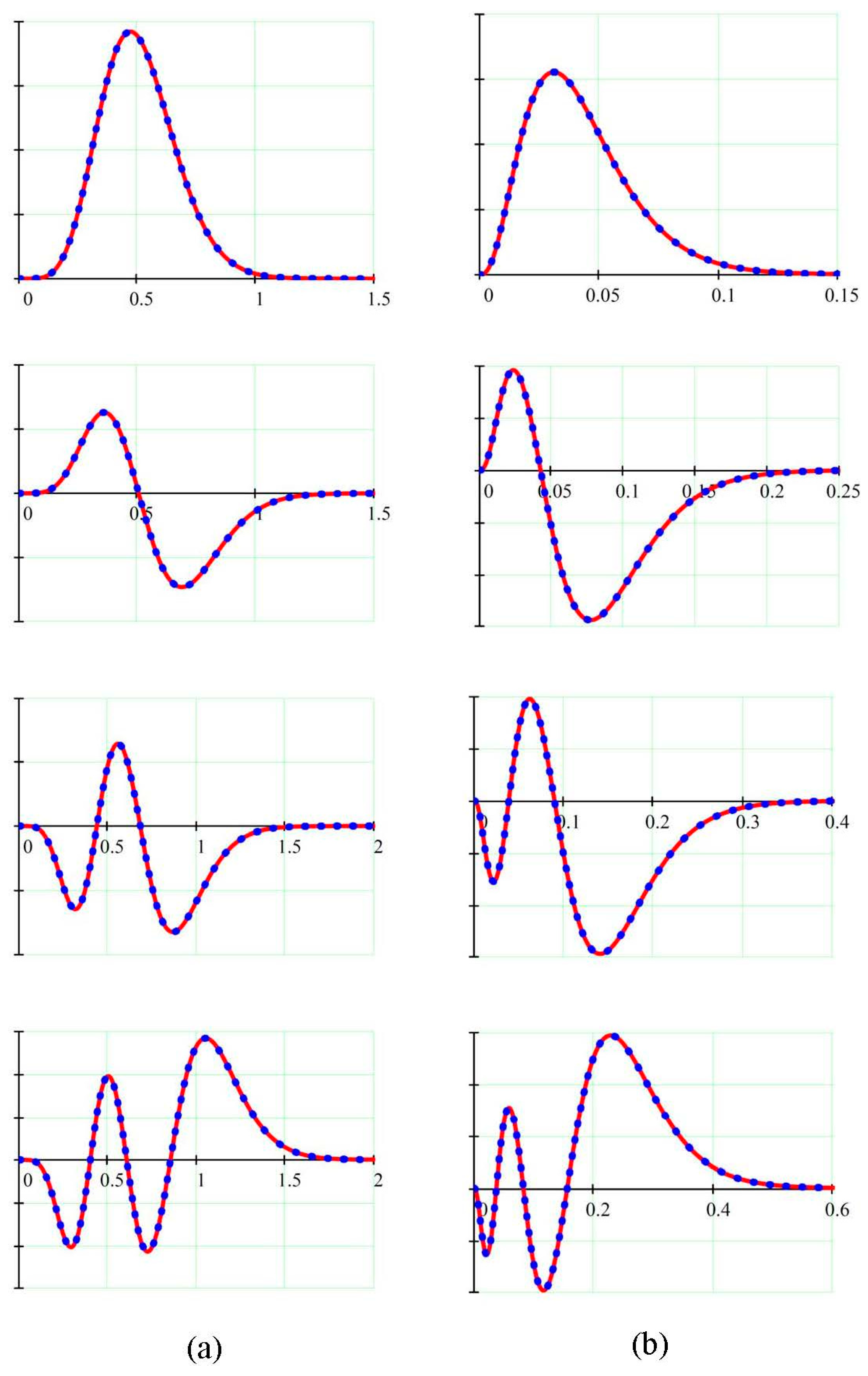
Figure 3a is a plot of the un-normalized bound state wavefunctions corresponding to the energy spectrum in Table 1. The red solid trace is the finite-series approximation (15), whereas the superimposed blue dotted trace is produced by a robust numerical routine that gives a highly accurate evaluation of the wavefunction. The routine evaluates a normalized eigenvector of the matrix wave equation using the corresponding eigenvalue in addition to a set of eigenvalues of an abbreviated submatrix. Such evaluation avoids direct computation of eigenvectors of matrices that could result in reduced accuracy and/or convergence, especially for large matrix sizes. The accuracy is further enhanced due to the tridiagonal matrix representations of the wave operator in the TRA. In such representations, one is at liberty to utilize various robust computational packages specialized for use with such matrices in which Gaussian quadrature, continued fractions, and other tools are available. The figure shows a very good match with about $3\times {10}^{-4}$ average deviation (defined as the absolute difference between the two traces divided by their sum over the entire range).

3. TRA Solution of the Potential Model (1b)

We repeat the same treatment in Section 2 for the potential model $V_{\mathrm{II}}(x)$. However, we choose the following coordinate transformation and basis parameters:

$$y(x)=2{\left[(x/a)+1\right]}^2-1, 2\alpha =\mu +1, 2\beta =-\nu -\frac{1}{2}.$$

(16)

Subsequently, the action of the wave operator on the basis elements $\mathcal{D}|{\varphi }_n\rangle$ becomes the confluent Heun equation [8]. Using the differential equation of the R-Jacobi polynomial (A1), this equation reduces to the following:

$$\begin{array}{c}\mathcal{D}|{\varphi }_n(y)\rangle =-\frac{2}{a^2}\frac{{(y-1)}^{\alpha -1}}{{(y+1)}^{\beta }}\{\frac{{\mu }^2-1}{y-1}-\frac{{\nu }^2-\frac{1}{4}}{y+1}+\frac{1}{2}{\left(2n+\mu +\nu +1\right)}^2-\frac{1}{8}\\ -\frac{2A}{y-1}+\frac{2B}{y+1}-C+\frac{\epsilon }{2}\left(y-1\right)\}{J}_n^{(\mu ,\nu )}(y)\end{array}$$

(17)

The TRA constraint (5) and the recursion relation of the R-Jacobi polynomials (A3) dictate that we assign the following values to the R-Jacobi polynomial parameters:

$${\mu }^2=2A+1, {\nu }^2=2B+\frac{1}{4}.$$

(18)

Reality dictates that $A\ge -\frac{1}{2}$ and $B\ge -\frac{1}{8}$. Moreover, the polynomial parameters inequalities $\mu >-1$ and $\mu +\nu <-2N-1$ dictate that $\mu =\sqrt{2A+1}$ and $\nu =-\sqrt{2B+\frac{1}{4}}$. This also shows that the maximum number of bound states that could be obtained by the TRA solution, $N+1$, becomes $\lfloor \frac{1}{2}\left(\sqrt{2B+\frac{1}{4}}-\sqrt{2A+1}-1\right)\rfloor +1$. With these choices of basis parameters, Equation (17) becomes:

$$\mathcal{D}|{\varphi }_n\rangle =-\frac{1}{a^2}\frac{{(y-1)}^{\alpha -1}}{{(y+1)}^{\beta }}\left[{\left(2n+\mu +\nu +1\right)}^2-\frac{1}{4}-\left(2C+\epsilon \right)+\epsilon y\right]J_n^{(\mu ,\nu )}(y).$$

(19)

Using the three-term recursion relation for the R-Jacobi polynomials (A3) in this equation and comparing the result to the TRA constraint (5), one obtains:

$$W(y)=\frac{-E}{y-1},$$

(20a)

$$d_n=\left[{\left(2n+\mu +\nu +1\right)}^2-\frac{1}{4}-\left(2C+\epsilon \right)\right]\frac{1}{\epsilon }+\frac{{\nu }^2-{\mu }^2}{(2n+\mu +\nu )(2n+\mu +\nu +2)},$$

(20b)

$$b_n=\frac{2(n+1)(n+\mu +\nu +1)}{(2n+\mu +\nu +1)(2n+\mu +\nu +2)}, c_n=\frac{2(n+\mu +1)(n+\nu +1)}{(2n+\mu +\nu +2)(2n+\mu +\nu +3)}.$$

(20c)

Consequently, the recursion relation (5), written in terms of $\left\{P_n\right\}$ and defined in Equation (13), becomes identical to Equation (A8) of the TRA polynomial ${\tilde{H}}_n^{(\mu ,\nu )}(z;\gamma ,\theta )$ with the following parameter and argument relations:

$$z^2=\frac{4}{C(C+\epsilon )}, {\gamma }^2=\frac{1}{16}, \cosh \theta =\frac{\epsilon +2C}{-\epsilon }.$$

(21a)

The condition that $\cosh \theta \ge 1$ dictates that $-C<\epsilon <0$ is the same condition that guarantees the reality of z. On the other hand, for $\epsilon <-C$, comparing the recursion relation (5), written for $\left\{P_n\right\}$, to Equation (A7), we conclude that $P_n=H_n^{(\mu ,\nu )}(z;\gamma ,\theta )$ with

$$z^2=\frac{-4}{C(C+\epsilon )}, {\gamma }^2=\frac{1}{16}, \cos \theta =\frac{\epsilon +2C}{-\epsilon }.$$

(21b)

Finally, the kth bound state wavefunction with energy $E_k={\epsilon }_k/a^2$ is written as the following finite series for $-C<{\epsilon }_k<0$:

$${\psi }_k(x)=2^{\frac{\mu +\nu }{2}}{}^{+\frac{3}{4}}{f}_0(z_k){\left(\frac{x}{a}+1\right)}^{\nu +\frac{1}{2}}{\left[{\left(\frac{x}{a}\right)}^2+2\frac{x}{a}\right]}^{\frac{\mu +1}{2}}{\displaystyle \sum _{n=0}^N{G}_n^{-1}{\tilde{H}}_n^{(\mu ,\nu )}\left(z_k;\frac{1}{4},{\theta }_k\right)J_n^{(\mu ,\nu )}(y)}.$$

(22a)

On the other hand, for ${\epsilon }_k<-C$, the wavefunction becomes:

$${\psi }_k(x)=2^{\frac{\mu +\nu }{2}}{}^{+\frac{3}{4}}{f}_0(z_k){\left(\frac{x}{a}+1\right)}^{\nu +\frac{1}{2}}{\left[{\left(\frac{x}{a}\right)}^2+2\frac{x}{a}\right]}^{\frac{\mu +1}{2}}{\displaystyle \sum _{n=0}^N{G}_n^{-1}{H}_n^{(\mu ,\nu )}\left(z_k;\frac{1}{4},{\theta }_k\right)J_n^{(\mu ,\nu )}(y)},$$

(22b)

where $\mu =\sqrt{2A+1}$, $\nu =-\sqrt{2B+\frac{1}{4}}$, $G_n$ is defined in Equation (13), and $z_k$ and ${\theta }_k$ are defined in Equations (21a,b), respectively. The physical properties of the system are obtained from those of the TRA polynomials $H_n^{(\mu ,\nu )}(z;\gamma ,\theta )$ and ${\tilde{H}}_n^{(\mu ,\nu )}(z;\gamma ,\theta )$, which have yet to be obtained and remain an open problem in orthogonal polynomials.

Table 2. The negative of the complete energy spectrum (in units of $1/a^2$) for the potential $V_{\mathrm{II}}(x)$ obtained using LMM and HMD techniques for the potential parameter values: $\left\{a,A,B,C\right\}=$ $\left\{1,10,1000,500\right\}$ making $N=19$. For the LMM, the variational parameter $h=0.0028$ and a grid size $M=100$ are used, whereas for the HMD, the scale parameter $\lambda =250$ and a matrix size $M=100$ are used.

n	HMD	LMM
0	3035.684 174 172 442	3035.684 174 170 930
1	1230.873 985 966 404	1230.873 985 965 147
2	482.923 837 697 235	482.923 837 696 618
3	134.670 968 410 057	134.670 968 409 830

shows the full energy spectrum of $V_{\mathrm{II}}(x)$ for the given set of values of the potential parameters obtained using LMM and HMD. A comparison of the results listed in Table 1 and Table 2 shows that our calculation with $V_{\mathrm{II}}(x)$ is less accurate than that with $V_{\mathrm{I}}(x)$. We believe that this accuracy deficiency is most likely due to the long range $1/x$ singularity present in $V_{\mathrm{II}}(x)$ but not $V_{\mathrm{I}}(x)$. To give a pictorial representation demonstrating this deficiency, in Figure 4 we show the two potential plots with the energy spectrum superimposed. One can observe three features that contribute to the computational difficulty:

(1)

$V_{\mathrm{II}}(x)$ is deeper, sharper, and has a slower decay compared to $V_{\mathrm{I}}(x)$;

(2)

The ground state from the bottom of the potential $V_{\mathrm{II}}(x)$ is much higher when compared to $V_{\mathrm{I}}(x)$;

(3)

The reduction in the energy spacing of the $V_{\mathrm{II}}(x)$ spectrum is much more rapid when compared to $V_{\mathrm{I}}(x)$.

Figure 3b is a plot of the un-normalized bound state wavefunctions corresponding to the energy spectrum shown in Table 2. The red solid trace is the finite-series approximation (22), whereas the superimposed blue dotted trace is produced by a robust numerical routine that gives a highly accurate evaluation of the wavefunction. The figure shows quite a good match, with about a $3\times {10}^{-4}$ average deviation (defined as the absolute difference between the two traces divided by their sum over the entire range).

4. Conclusions

The potential plots in Figure 1 and the spectral phase diagram in Figure 2 show that the two potential functions, introduced in this paper, have a rich structure. Therefore, these potentials can be used to model various physical systems with a wide range of structural and dynamical properties. These two potentials do not belong to the class of exactly solvable quantum mechanical problems. Nonetheless, we were able to use the tridiagonal representation approach and obtain a reasonably accurate approximation of the bound state solutions with the constraint that all potential parameters are positive. That is, the tridiagonal representation approach (TRA) solution space is confined to the green “B&R” region of the spectral phase diagram (SPD). We should also mention that for $C<0$, the TRA can also be used to obtain an approximation for the lowest $\lfloor -\frac{\mu +\nu +1}{2}\rfloor +1$ bound states. In the SPD, these solutions lie in the blue “B” region.

The shortcoming of the solution found here is that the analytic properties of the TRA polynomials $H_n^{(\mu ,\nu )}(z;\gamma ,\theta )$ and ${\tilde{H}}_n^{(\mu ,\nu )}(z;\gamma ,\theta )$, which contain all the physical properties of the system, are yet to be derived. This is a mathematical problem which goes beyond the scope of this work and the expertise of the authors. However, for the complete descriptions of the solution given by Equations (15) and (22), one needs only the corresponding energy eigenvalue $E_k$. We used two independent numerical routines to obtain a highly accurate evaluation of the complete energy spectrum, as shown in the tables.

We should also note that increasing the accuracy of our results requires us to increase the size of the basis, which is not possible in this problem since N is fixed by the values of the potential parameters A and B. In other finite TRA solutions where N depends on arbitrary basis parameter(s) and/or the energy, such an increase in accuracy is possible.

References

1. Alhaidari, A.D.; Bahlouli, H. Tridiagonal representation approach in quantum mechanics. Phys. Scr. 2019, 94, 125206. [Google Scholar] [CrossRef]
2. Alhaidari, A.D. Solution of the nonrelativistic wave equation using the tridiagonal representation approach. J. Math. Phys. 2017, 58, 072104. [Google Scholar] [CrossRef]
3. Alhaidari, A.D.; Aounallah, H. Construction of potential functions associated with a given energy spectrum—An inverse problem. II. Int. J. Mod. Phys. A 2020, 35, 2050159. [Google Scholar] [CrossRef]
4. Brau, F. Limits on the number of bound states and conditions for their existence. In Studies in Mathematical Physics Research; Benton, C.V., Ed.; Nova Science Publishers Inc.: Hauppauge, NY, USA, 2004; Chapter 1; Available online: https://dipot.ulb.ac.be/dspace/bitstream/2013/232876/3/2005_chapitre-livre.pdf (accessed on 20 July 2022).
5. Chadan, K.; Khuri, N.N.; Martin, A.; Wu, T.T. Bound states in one and two spatial dimensions. J. Math. Phys. 2003, 44, 406–422. [Google Scholar] [CrossRef]
6. Curtiss, D.R. Recent extensions of Descartes’ rule of signs. Ann. Math. 1918, 19, 251–278. [Google Scholar] [CrossRef]
7. Assi, I.A.; Alhaidari, A.D.; Bahlouli, H. Deformed Morse-like potential. J. Math. Phys. 2021, 62, 093501. [Google Scholar] [CrossRef]
8. Ronveaux, A. (Ed.) Heun’s Differential Equations; Oxford University Press Inc.: New York, NY, USA, 1995. [Google Scholar]
9. Chihara, T.S. An Introduction to Orthogonal Polynomials; Gordon and Breach, Science Publishers: New York, NY, USA, 1978; Available online: https://bayanbox.ir/view/1984196138202468281/Theodore.S.Chihara-An-introduction-to-orthogonal-polynomials.pdf (accessed on 20 July 2022).
10. Ismail, M.E.H. Classical and Quantum Orthogonal Polynomials in One Variable; Cambridge University Press: Cambridge, UK, 2005. [Google Scholar] [CrossRef]
11. Alhaidari, A.D. Open problem in orthogonal polynomials. Rep. Math. Phys. 2019, 84, 393–405. [Google Scholar] [CrossRef]
12. Assche, W.V. Solution of an open problem about two families of orthogonal polynomials. SIGMA 2019, 15, 005. [Google Scholar] [CrossRef]
13. Baye, D.; Hesse, M.; Vincke, M. The unexplained accuracy of the Lagrange-mesh method. Phys. Rev. E 2002, 65, 026701. [Google Scholar] [CrossRef] [PubMed]
14. Baye, D. The Lagrange-mesh method. Phys. Rep. 2015, 565, 1–107. [Google Scholar] [CrossRef]
15. Romanovski, V. Sur quelques classes nouvelles de polynomes orthogonaux. Comp. Rend. L’Acad. Sci. Paris 1929, 188, 1023–1025. Available online: https://gallica.bnf.fr/ark:/12148/bpt6k31417/f1023.item (accessed on 20 July 2022).
16. Lesky, P.A. Endliche und unendliche Systeme von kontinuierlichen klassichen Orthogonalpolynomen. Z. Angew. Math. Mech. / J. Appl. Math. Mech. 1996, 76, 181–184. [Google Scholar] [CrossRef]
17. Lesky, P.A. Vervollstandigung der klassischen Orthogonalpolynome durch Erganzungen zum Askey-Schema der hypergeometrischen orthogonalen Polynome. Sb. Öst. Akad. Wiss. Math. Nat. Kl. 1995, 204, 151–166. [Google Scholar]
18. Natanson, G. Biorthogonal differential polynomial system composed of X-Jacobi polynomials from different sequences. arXiv 2018, arXiv:1801.10216. [Google Scholar] [CrossRef]
19. Chen, M.-P.; Srivastava, H.M. Orthogonality relations and generating functions for Jacobi polynomials and related hypergeometric Functions. Appl. Math. Comput. 1995, 68, 153–188. [Google Scholar] [CrossRef]
20. Askey, R. An integral of Ramanujan and orthogonal polynomials. J. Indian Math. Soc. 1987, 51, 27–36. Available online: https://www.informaticsjournals.com/index.php/jims/article/view/22015 (accessed on 20 July 2022).
21. Routh, E.J. On some properties of certain solutions of a differential equation of the second order. Proc. Lond. Math. Soc. 1885, 16, 245–262. [Google Scholar] [CrossRef] [Green Version]
Figure 1. The two potential functions V I ( x ) (1a) and V II ( x ) (1b) (in units of A) for several values of the associated parameters: (a) V I ( x ) with C = 5 A and several values of B, and (b) V II ( x ) with C = 2 A and several values of B.
Physics 04 00070 g001
Figure 2. The spectral phase diagram (SPD) for: (a) V I ( x ) , and (b) V II ( x ) . The diagram shows the distribution of the energy spectrum (scattering states “S”, bound states “B”, resonances “R”, and regions where both bound states and resonances can occur (“B&R”) as a function of the potential parameters.
Physics 04 00070 g002
Figure 3. The un-normalized wavefunctions corresponding to the energy spectrum of: (a) V I ( x ) in Table 1, and (b) V II ( x ) in Table 2. The horizontal x-axis is in units of a. The plots from top to bottom are ψ 0 ( x ) , …, ψ 4 ( x ) . The red solid trace is the TRA finite-series approximation, whereas the superimposed blue dotted trace is the result of a robust numerical routine that gives a highly accurate evaluation of the wavefunction. See text for details.
Physics 04 00070 g003
Figure 4. The two potential functions with their energy spectra superimposed. The physical parameters and results of Table 1 and Table 2 are used. One can observe the three features of V II ( x ) (b), mentioned at the end of Section 3, which are the source of deficiency in the computational accuracy compared to V I ( x ) (a).
Physics 04 00070 g004