Probability Distributions for Track Fitting and the Advanced Lucky Model

Abstract

Probability distributions for the center of gravity are fundamental tools for track fitting. The center of gravity is a widespread algorithm for position reconstruction in tracker detectors for particle physics. Its standard use is always accompanied by an easy guess (Gaussian) for the probability distribution of the positioning errors. This incorrect assumption degrades the results of the fit. The explicit error forms evident Cauchy–Agnesi tails that render the use of variance minimizations problematic. Therefore, it is important to report probability distributions for some combinations of random variables essential for track fitting: $x=\xi /(\xi +\mu )$, $y=(\xi -\mu )/\left[2(\xi +\mu )\right]$, $w=\xi /\mu$, $x=\theta (x_3-x_1)(-x_3)/(x_3+x_2)+\theta (x_1-x_3)x_1/(x_1+x_2)$ and $x=(x_1-x_3)/(x_1+x_2+x_3)$. The first two are partial forms of the two strip center of gravity. The fourth is the complete two strip center of gravity, and the fifth is a partial form of the three strip center of gravity. For the complexity of the forth equation, only approximate expressions of the probability are allowed. Analytical expressions are calculated assuming $\xi$, $\mu$, $x_1$, $x_2$ and $x_3$ independent Gaussian random variables. The analytical form of the probability for the two strip center of gravity allows one to construct an approximate proof for the lucky model of our previous paper. This proof also suggests how to complete the lucky model by its absence of a scaling constant, relevant to combine different detector types. This advanced lucky model (the super-lucky model) can be directly used in trackers composed of non-identical detectors. The construction of the super-lucky model is very simple. Simulations with this upgraded tool also show resolution improvements for a combination of two types of very different detectors, near to the resolutions of the schematic model.

1. Introduction

The top resolutions in track fitting, discussed in [1,2,3], require special types of probability density functions (PDFs) for their realizations. The maximum likelihood, used to obtain the top resolutions, implies the handling of products of the observation PDFs (likelihood), one PDF for each observation of the fit. Such PDFs must have analytical expressions, appositely tuned on the statistical properties of the used signals. In our case, signals were released by minimum ionizing particles (MIPs) in silicon micro-strip detectors. In fact, a careful observation of the simulated data evidences the impossibility to reproduce the scatter-plots with a single variance (homoscedasticity). The homoscedasticity of the observations implies immense simplification of the fitting problem: the variances of the observations disappear from the equations for the least-squares. Those equations can be applied to any type of fitting problem. The homoscedasticity is a fundamental assumption of mathematical statistics, as repeatedly recalled in [4]. The failure of this key point of mathematical statistics imposes a completely different strategy. 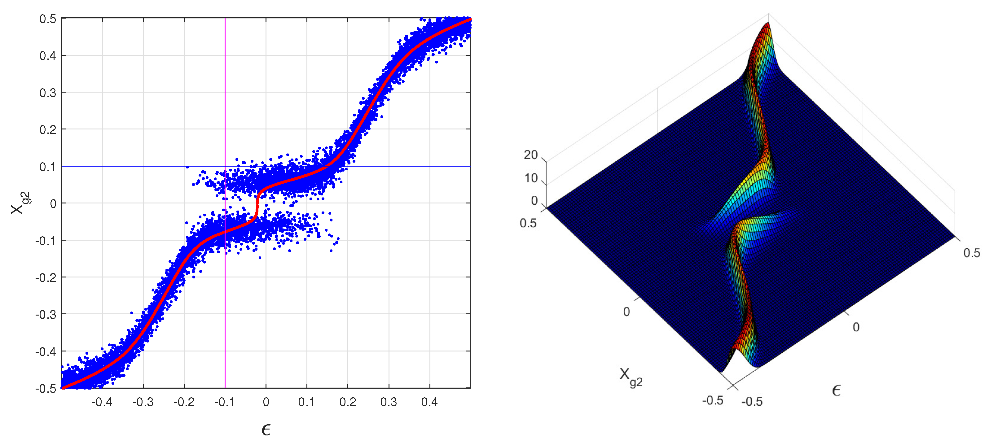The properties of the observations (hits) must be carefully studied to extract the essential information to achieve the fit optimality [5]. The scatter-plots, which provided a hint to these studies, were those of [6], showing samples of center of gravity (COG) of MIP signals as a function of the MIP impact points, ($\epsilon$).

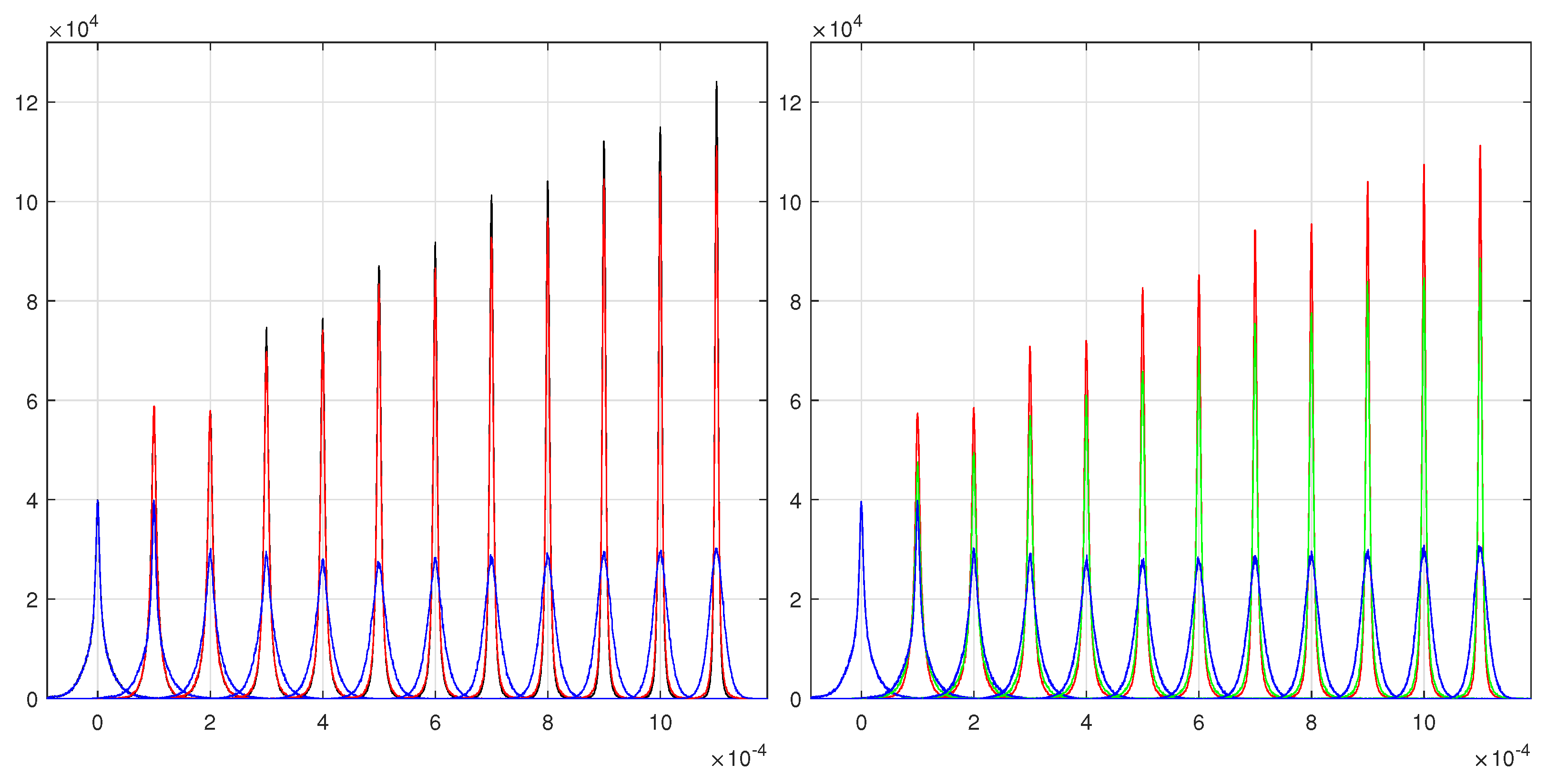
To explore the relevance of additional pieces of information, those simulations were used to produce seven very rough approximations of the PDFs as functions of $\epsilon$ for a fixed interval of COG values. Those rough PDFs were used in a maximum likelihood search of fitted parameters of MIP straight tracks. The evident improvement of the parameter distributions convinced us about the importance of the additional pieces of information. A feature was particularly convincing: the unexpected richness of exact values, absent in the standard fits (homoscedastic least squares). This feature was clearly evident as narrow peaks in all our simulations. However, to effectively use those hints, the rough PDFs need to be replaced with accurate forms such as those derived in the following and used in [1,2,3]. In addition, we demonstrated in Refs. [5,7] that the usual fitting methods are non-optimal just for the neglect of the variance differences of the hits. Those studies proved that the variances of the fitted parameters, given by the standard fits, are always greater than the variances obtained by weighted fits with the hit variances as weights. The demonstrations are perfectly consistent with our early empirical results.

The aim of this study is to complete the previously employed methods giving the derivations and the explicit expressions of the PDFs essential to obtain our previous results. The implied PDFs are those calculated for the center of gravity (COG) algorithm. The COG algorithm is an easy and efficient positioning algorithm that is widely used in particle physics and in many other technological problems. The generic COG definition is ${\sum }_j{E}_j{X}_j/{\sum }_j{E}_j$, where $\left\{E_j\right\}$ are the signals of a cluster inserted in the COG and $\left\{X_j\right\}$ denote their positions. The different selections of the signals, inserted in the COG expression, generate positioning algorithms with different analytical and statistical properties. Our special attention is directed to the two strip COG (COG₂) for its minimal noise and usefulness for tracks at orthogonal incidence (direction with the worst resolution). The COG₂ is computed with the signals of the leading strip (seed) and the maximum of the two contiguous strips. The corresponding PDF has a typical gap, the explanation of this feature and examples are reported in [8]. It is just this typical feature that renders very complicated the calculation and very long the equation of the PDF for the COG₂. Nevertheless, the COG₂ PDF is extensively used in the simulations of [2,3] with very large improvements for the resolutions of the track parameters (up to a factor three for the most favorable cases). Although our attention is focalized on COG₂, other COG PDFs are calculated as well, and few of them are frequently used in our approaches. However, the COG PDFs are only a part of the probabilities for track fitting, the other part is the insertion of the functional dependence on $\epsilon$. Completed with the particle impact point ($\epsilon$), the PDF can take into account the signal-to-noise ratio of each strip and correct the COG systematic errors. The insertion of the $\epsilon$ functional dependence requires the exploration and filtering of special types of random processes and the availability of large sets of homogeneous data [2]. Further details about the handling of these types of random processes will be discussed elsewhere.

As a non-trivial by product, the analytical expression of the COG₂ PDF also allows us to discuss an approximate demonstration for the lucky model [1]. The same equation also consents to an extension of the lucky model to trackers formed with non-identical detectors (a declared limitation for the lucky model in [1]).

In Section 2, the necessity to go beyond the standard (homoscedastic) least squares method is illustrated and the simplest forms of COG PDFs are reported. In the following, the least squares method, which uses the equations for homoscedastic systems, is called “standard least squares.” Section 3 and Section 4 are devoted to the complete COG₂ PDF and the PDF for the three strip COG. Applications of these results are reported in Section 5, with proofs and extensions of the lucky model. Section 6 contains the conclusions. Appendix A gives a derivation of a partial COG₂ PDF from the cumulative probability distribution and Appendix B reports on a better approximation of the COG₂ PDF. These results are obtained with the extended use of MATHEMATICA [9] and verified in many realistic cases with MATLAB [10] simulations.

2. Definition of the Problem

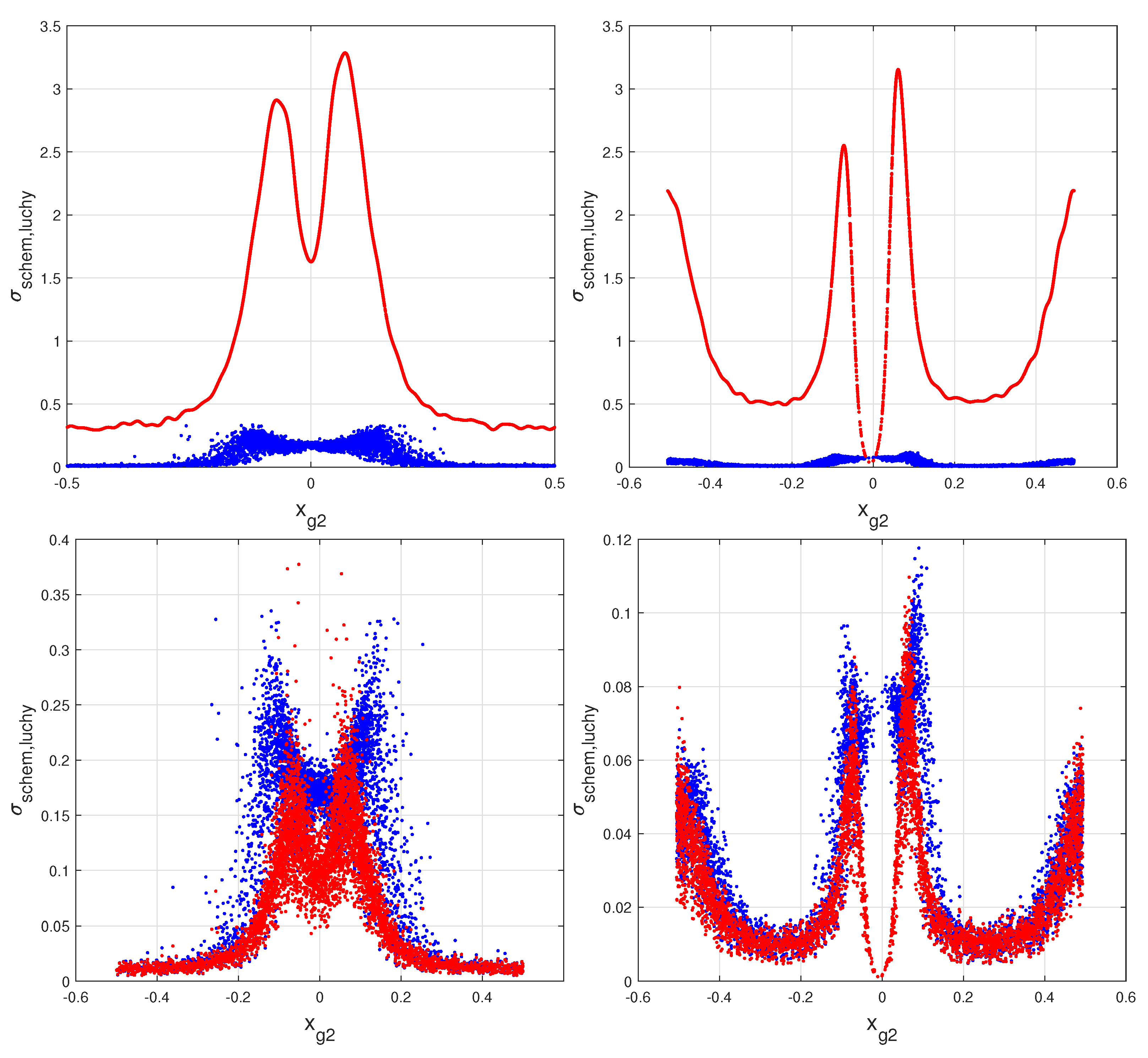
The peculiar non-uniformity (heteroscedasticity) of the point distributions in the scatter plots of COG simulations are easily observed, (as in [2,6] and in the figures shown in this study). In [2], this heteroscedasticity is demonstrated with the definition of an effective variance for each hit and with the distributions of the samples of these values. The plots of those distributions substantially differ from a horizontal line, the obvious result for an identical variance for all hits (homoscedasticity). Therefore, the hypothesis of homoscedasticity for the positioning errors must be ruled out in favor of more realistic assumptions. In fact, the variance reduction, introduced by the distinction of good or excellent hits (heteroscedasticity) on a track containing two or more hits of such types, is easily grasped. This is the reason for the evident richness of the exact values of the heteroscedastic fits, absent in the standard least squares. The distributions of the hit effective standard deviations also show trends surprisingly similar to the COG histograms. This similarity consents the definition of a sub-optimal model (the lucky model [1]) for the hit variances that introduce good improvements in the fitting results, without the complications of the full calculation.

The corrections of the hit properties, due to the differences of the detector technologies along the lines of Ref. [11], are small steps in the right direction but absolutely insufficient. Experimental indications about the differences of the hit resolutions are reported in [12]. However, the Landau distribution of the charge released by a MIP is another well known experimental fact, adding further differences to the hit properties and definitively suppressing the homoscedasticity. Instead, the maximum likelihood method involves all the available information contained in the data, and it is able to obtain drastic improvements of the track parameters also in presence of outliers [2]. This ability to handle outliers is a consequence of the tails of PDFs. As previously discussed, another important feature is introduced by the different quality of hit PDFs. 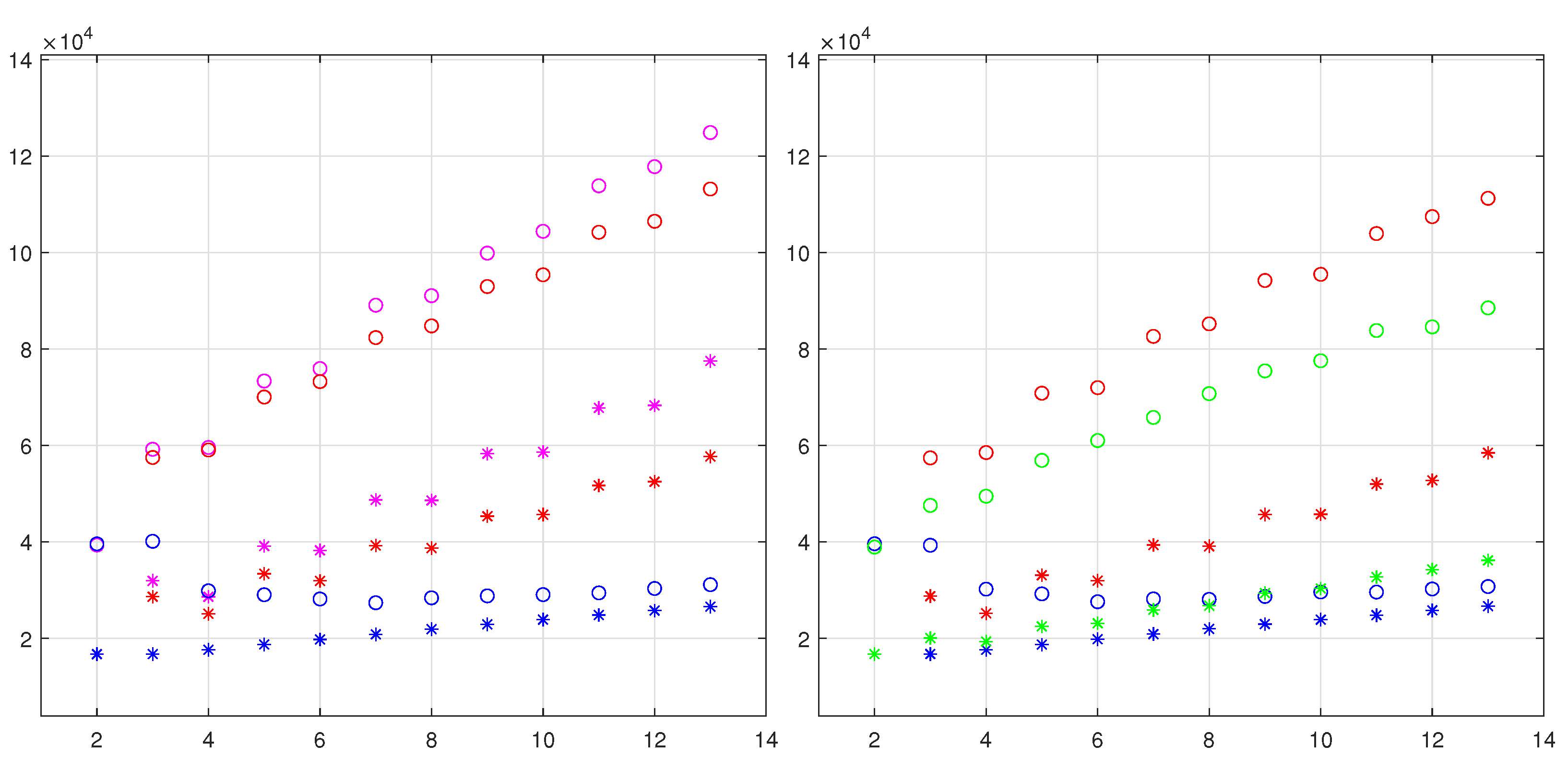Two goods (or excellent) hits suffice for a good (or excellent) straight track fit as in [2], or three of them for momentum reconstruction in a known homogeneous magnetic field as in [3]. The probability of good (or excellent) hits grows proportionally to the number N of hits (detecting layers) per track [1,5,7]. Therefore, the pool of the track parameters is enriched at this rate (≈linear in N) for a range of N-values of interest for tracker physics. Instead, the standard least squares, not accounting for the hit differences, grows as $\approx \sqrt{N}$. This is a very slow growth compared with the linear one, implying a waste of tracker resolution and an increase of tracker complexity.

In spite of the proofs of the maximum likelihood as the best fitting method, intrinsic difficulties limit its use. For very complex trackers, the full machinery of the maximum likelihood could be beyond reasonable computing resources. Although the schematic model [2] substitutes the maximum likelihood method with a weighted least squares, the computing of the effective hit variances also requires large processing time. The lucky model of Ref. [1] and its advanced version can be an easy substitute. Evidently, each departing step from the maximum likelihood adds a loss of resolution. It must be remembered that the schematic model, the lucky model, and its advanced form are ineffective with the outliers.

The required analytical expressions of the PDFs have the general functional forms $P(\epsilon ,x_{g_n})$, where, $x_{g_n}$ is a generic COG with n-strips. The conditional probabilities, $P\left(\epsilon \right|x_{g_n})$ and $P\left(x_{g_n}\right|\epsilon )$, are connected with the marginal probabilities, $P\left(x_{g_n}\right)$ and $P\left(\epsilon \right)$ [13]:

$$P\left(\epsilon \right|x_{g_n})P\left(x_{g_n}\right)=P(\epsilon ,x_{g_n})=P\left(x_{g_n}\right|\epsilon )P\left(\epsilon \right).$$

The constant probability of the impact point $\epsilon$ is assured by

$$P\left(\epsilon \right)={\int }_{-\infty }^{+\infty }P(\epsilon ,x_{g_n})\mathrm{d}{x}_{g_n}=1,$$

(1)

and it is consistent with the assumption of uniformity and normalization on a strip.

The Kolmogorov axioms [13] attribute to the cumulative probability distribution a fundamental role to calculate the PDF. The cumulative probability distribution for a continuous case is given by integrations on the appropriate portion of the plane, or the space, as required by the geometry of the problem. Differentiating the cumulative probability distribution produces the PDF. This method becomes extremely long with complicated algorithms. However, our first approach was modeled on the ratio of two random variables of [13], and we used the cumulative distributions for all the considered PDFs, from the simplest to the most complex one. This very long set of integrals is quite tedious, to be reported in a paper. This is the principal reason for the delay of this report. Here, a different approach is utilized, very direct and flexible, with the use of Dirac $\delta$-functions and Heaviside $\theta$-functions, operating directly on the PDFs of the strip noise; an assay was given in [3]. This method is a variance of the Fermi “golden rule 1” that is used for the cross-section calculations (or diffusion probabilities), and it recovers the results of our geometric approaches. However, Gauss [14] gives similar generic expressions as obtained after the $\delta$-integration, but we found that old fundamental paper only recently. To underline the consistency with the geometric approach, the first part of the COG₂ PDF is obtained with the cumulative probability distribution in Appendix B.

The random signals of our interest are modeled on the charges released on the strips by the hitting MIPs. The signals are corrupted by additive random noises produced by the rest of the acquisition system. The data are at their final elaboration procedure (calibration, pedestal, common noise suppression, etc.) and are ready to be used in a positioning algorithm of any type. The stream of primary charges, released by a MIP, diffuses in the detector toward a cluster of strips. The charges, collected by a strip, are correlated with those, collected by the cluster. The distributions of the charges in the cluster depend, among other parameters such as particle direction and total released charges, on the MIP impact point. Hence, the $\epsilon$ dependence of $P(\epsilon ,x_{g_n})$ must be contained in the strip signal $a_i$. The signals $a_i$ are considered as parameters, and the PDF will be expressed in the form $P(\left\{a_i\right\},x_{g_n})$, where $\left\{a_1\right\}$ is the set of strips inserted in $x_{g_n}$. The variable $x_{g_n}$ is abandoned for a simpler $x_{g_n}$ ! x. The strip size is always taken to be one, and this is the length scale of the system (all the implied lengths are divided by the strip widths). The parameters, $\left\{a_i\right\}$, can be expressed in any dimensional units consistent with those of the noise $\left\{{\sigma }_i\right\}$ (we use directly the ADC (analog-to-digital converter) counts.) The variable x turns out to be a pure number as the PDFs.

Each strip has its own random additive noise uncorrelated with that of any other strip. In strips without MIP signals, the strip noise is well reproduced with a Gaussian PDF. Thus, the PDFs for the signal plus noise of the strip i become:

$$P_i\left(z\right)=\frac{1}{\sqrt{2\pi }{\sigma }_i}exp\left[-\frac{{(z-a_i)}^2}{2{\sigma }_i^2}\right], i=1,2,\dots ,n.$$

(2)

The Gaussian mean values $\left\{a_i\right\}$ are the (noiseless) charges, collected by the strips, and are positive numbers (we assume to have signals from real particles). The parameters $\left\{{\sigma }_i\right\}$ are the standard deviations of the additive zero-average Gaussian noise.

2.1. Probability for the Ratio $x=\xi /(\xi +\mu )$

The first explored PDF is the distribution of the random values of x with $x=\xi /(\xi +\mu )$. This expression has the structure of a COG with the origin of the reference system in the center of the strip 2 ($\mu$ random variable) and another signal on the right strip 1 ($\xi$ random variable). This form of COG is the right part of the full COG₂ algorithm. Due to its limitation to only two random variable $\{\xi ,\mu \}$, it is a first step toward more complex PDFs. The derivation of the PDF for $P_{x{g}_{2}R}\left(x\right)$ with the cumulative distribution is illustrated in Appendix B However, this PDF can be rapidly obtained with this method:

$$P_{x{g}_{2}R}\left(x\right)={\int }_{-\infty }^{+\infty }\delta \left(x-\frac{\xi }{\xi +\mu }\right)P_1\left(\xi \right)P_2\left(\mu \right)\mathrm{d}\xi \mathrm{d}\mu .$$

(3)

Integrating the $\delta$-function with $z=\xi +\mu$:

$${\int }_{-\infty }^{+\infty }F\left(z\right)\delta \left(x\pm \frac{\xi }{z}\right)\mathrm{d}z=F\left(\mp \frac{\xi }{x}\right)\frac{\left|\xi \right|}{x^2},$$

(4)

the expression for $P_{x{g}_{2}R}\left(x\right)$ is easily obtained:

$$P_{x{g}_{2}R}\left(x\right)=\frac{1}{x^2}{\int }_{-\infty }^{+\infty }{P}_1\left(\xi \right)P_2\left(\frac{1-x}{x}\xi \right)\left|\xi \right|\mathrm{d}\xi .$$

(5)

The heavy tails of a Cauchy–Agnesi-like distribution are evident; Equation (5) shows $1/x^2$ behavior for $x\to +\infty$, and the factor $(1-x)/x$ goes to $-1$. In this limit, the integral is convergent and different from zero. Identically for $x\to -\infty$. The singularity for $x=0$ is apparent because one integrand goes to zero for $x\to 0$ and can be removed with the coordinate transformation $z/x=\zeta$. However, it is useful to save the $1/x^2$ factor to remember the divergence of the variance for $P_{x{g}_{2}R}\left(x\right)$. The Gaussian integral is analytic for any x and $a_i$ and has the following form:

$$\begin{array}{cc}\hfill P_{x{g}_{2}R}\left(x\right)& =\frac{a_2(1-x){\sigma }_1^2+a_{1}x{\sigma }_2^2}{\sqrt{2\pi }{[{(1-x)}^2{\sigma }_1^2+x^2{\sigma }_2^2]}^{3/2}}exp\left[-{\left(\frac{a_1}{a_1+a_2}-x\right)}^2\frac{{(a_1+a_2)}^2}{2\left({\sigma }_1^2{(1-x)}^2+x^2{\sigma }_2^2\right)}\right]\hfill \\ & \times \mathrm{erf}\left[\frac{a_2(1-x){\sigma }_1^2+a_{1}x{\sigma }_2^2}{\sqrt{2}{\sigma }_1{\sigma }_2\sqrt{{(1-x)}^2{\sigma }_1^2+x^2{\sigma }_2^2}}\right]+exp\left(-\frac{a_1^2}{2{\sigma }_1^2}-\frac{a_2^2}{2{\sigma }_2^2}\right)\frac{{\sigma }_1{\sigma }_2}{\pi \left[{(1-x)}^2{\sigma }_1^2+x^2{\sigma }_2^2\right]}.\hfill \end{array}$$

(6)

The expression of the $P_{x{g}_{2}R}\left(x\right)$ shows some aspects that will be found often in the following. One can easily recognize, in Equation (6), part of the PDF reported in [3]. Equation (6) has a maximum for $x\approx a_1/(a_1+a_2)$. The maximum is the noiseless COG for this combination of variables and tends to eliminate the COG systematic error [8]. Around the maximum, $P_{x{g}_{2}R}\left(x\right)$ looks similar to a Gaussian. However, the exponential differs from a Gaussian for large x. The modulating term of the exponential is connected to the signal to noise ratio of the two strips. The positivity of the PDF is granted by the term $A\mathrm{erf}\left(A\right)$, which, for a not too small A, converges rapidly to $\left|A\right|$. Around zero, $A\mathrm{erf}\left(A\right)$ is a continuous differentiable function and differs from $\left|A\right|$ essentially for the cusp at $A=0$ of $\left|A\right|$. The range of the differences with respect to $\left|A\right|$ are of the order of ${\sigma }_1$ (or some weighted average with ${\sigma }_2$). This range is expected to be negligible, if the hit-detection algorithm works well and discards almost all the fake hits (with $a_i=0$). Thus, very often we will substitute $A\mathrm{erf}\left(A\right)$ with $\left|A\right|$.

The last term will be indicated as “Cauchy-like” term; it is very similar, but not identical, to a Cauchy-Agnesi PDF. This term survives also for $a_1=a_2=0$ and could be a probability of fake hits. It assures the strict positivity of the PDF. For $a_i\ne 0$, the Cauchy-like term is heavily suppressed by the negative exponents, quadratic in the strip signal-to-noise ratio.

The validity of this PDF is limited to one side of the COG₂ algorithm. The track reconstruction requires a rigid connection to the local reference system, which is naturally locked in the seed-strip center. Therefore, it is important to conserve a difference from the left strip, the central strip, and the right strip. The track impact point, $\epsilon$, can also be located outside the seed strip.

Another PDF, which composes the complete COG₂ PDF, contains the random variable $\beta$, the signal collected by strip 3 positioned to the left of strip 2. This PDF will be indicated as $P_{x{g}_{2}L}\left(x\right)$. As for $P_{x{g}_{2}R}\left(x\right)$, the strip 2 is the seed of the strip cluster. As always, the origin of the reference system is the center of strip 2. Now, x is given by the combination of random variables $-\beta /(\beta +\mu )$. The function $P_{x{g}_{2}L}\left(x\right)$ is obtained from Equation (6) with the substitution $a_1\to a_3$, ${\sigma }_1\to {\sigma }_3$ and $x\to -x$. We report here $P_{x{g}_{2}L}\left(x\right)$; often in the following, terms of this type will be indicated with the substitutions needed for their construction:

$$\begin{array}{cc}\hfill P_{x{g}_{2}L}\left(x\right)& =\frac{a_2(1+x){\sigma }_3^2-a_{3}x{\sigma }_2^2}{\sqrt{2\pi }{[{(1+x)}^2{\sigma }_3^2+x^2{\sigma }_2^2]}^{3/2}}exp\left[-{\left(\frac{a_3}{a_3+a_2}+x\right)}^2\frac{{(a_3+a_2)}^2}{2({\sigma }_3^2{(1+x)}^2+x^2{\sigma }_2^2)}\right]\hfill \\ & \times \mathrm{erf}\left[\frac{(1+x)a_2{\sigma }_3^2-a_{3}x{\sigma }_2^2}{\sqrt{2}{\sigma }_3{\sigma }_2\sqrt{{(1+x)}^2{\sigma }_3^2+x^2{\sigma }_2^2}}\right]+exp\left[-\frac{a_3^2}{2{\sigma }_3^2}-\frac{a_2^2}{2{\sigma }_2^2}\right]\frac{{\sigma }_3{\sigma }_2}{\pi [{(1+x)}^2{\sigma }_3^2+x^2{\sigma }_2^2]}.\hfill \end{array}$$

(7)

The small x approximation is now:

$$P_{x{g}_{2}L}\left(x\right)=\frac{|a_2|}{\sqrt{2\pi }}\frac{exp\left[-{\left(x+\frac{a_3}{a_3+a_2}\right)}^2\frac{{(a_3+a_2)}^2}{2\left({\sigma }_3^2{(1+x)}^2\right)}\right]}{{\sigma }_3{(1+x)}^2}.$$

The approximation of $P_2[z(-1-x)/x]$ as a Dirac $\delta$-function in the integration of Equation (5) does not reproduce the Cauchy-like term. The factor $(1+x)$ is retained, being contained in the argument of the $\delta$-function. Its role is essential to obtain the maximum of $P_{x{g}_{2}L}\left(x\right)$ in the expected position $-a_3/(a_3+a_2)$ of its noiseless COG.

2.2. Probability Distribution for $y=\frac{\xi -\mu }{2(\xi +\mu )}$

Another type of COG₂ algorithm is of frequent use, for example, in [15]. The main difference of this combination of random variables, from previous expressions, is a translation with respect to the standard reference system (centered in the middle of the strip 2). Now, the reference system is centered on the right border of the strip 2. This COG₂ algorithm has the following form:

$$y=x-\frac{1}{2}=\frac{\xi -\mu }{2(\xi +\mu )}.$$

(8)

Although this is another direct transformation of Equation (6), we report its general form and the case of Gaussian PDF for completeness:

$$P_G\left(y\right)=P_{x{g}_{2}R}\left(y+\frac{1}{2}\right)={\int }_{-\infty }^{+\infty }{P}_1\left(\xi \right)P_2\left(\frac{1-2y}{1+2y}\xi \right)\frac{\left|\xi \right|}{{(y+1/2)}^2}\mathrm{d}\xi .$$

(9)

In the form of $P_G\left(y\right)$, we directly use the substitution of $A\mathrm{erf}\left(A\right)$ with $\left|A\right|$. In any case, $A\mathrm{erf}\left(A\right)$ is easily obtained from Equation (6):

$$\begin{array}{cc}\hfill P_G\left(y\right)& =\frac{4|a_2(1-2y){\sigma }_1^2+a_1(1+2y){\sigma }_2^2|}{\sqrt{2\pi }{\left[{(1-2y)}^2{\sigma }_1^2+{(1+2y)}^2{\sigma }_2^2\right]}^{3/2}}exp\left[-{\left(\frac{a_1-a_2}{2(a_1+a_2)}-y\right)}^2\right.\hfill \\ & \times \left.\frac{2{(a_1+a_2)}^2}{({\sigma }_1^2{(1-2y)}^2+{(1+2y)}^2{\sigma }_2^2)}\right]\hfill \\ & +exp\left[-\frac{a_1^2}{2{\sigma }_1^2}-\frac{a_2^2}{2{\sigma }_2^2}\right]\frac{4{\sigma }_1{\sigma }_2}{\pi \left[{(1-2y)}^2{\sigma }_1^2+{(1+2y)}^2{\sigma }_2^2\right]}.\hfill \end{array}$$

(10)

With a similar transformation, the PDF for $y=x+1/2$ can be obtained; here, the reference system is centered on the left border of strip 2 with strip 3. A discussion of the variance of y for small errors is given in [16], although the variance is an ill defined parameter due to the Cauchy–Agnesi-like tails of the PDF. In this case, the results depend on the assumptions introduced.

These PDFs have simple analytical forms; they are defined in reference systems that depend on the signal in the second strip. Their use in maximum likelihood search, could imply heavy complications in the exploration of the likelihood surface. In fact, to allow for the maximum to be outside the two strips of the PDF, another function must be introduced with a different reference system.

2.3. Probability Distribution for $w=\xi /\mu$

As a final use of Equation (5), we apply it to obtain the PDF for the ratio of random variables $w=\xi /\eta$. Now it reads:

$$x=\frac{\xi }{\xi +\mu },w=\xi /\mu ,x=\frac{w}{1+w},P_{\xi /\mu }\left(w\right)=P_{x{g}_{2}R}\left(\frac{w}{1+w}\right)\frac{1}{{(1+w)}^2}.$$

(11)

The integral expression of $P_{\xi /\mu }\left(w\right)$ becomes:

$$P_{\xi /\mu }\left(w\right)=\frac{1}{w^2}{\int }_{-\infty }^{+\infty }{P}_1\left(z\right)P_2\left(\frac{z}{w}\right)\left|z\right|\mathrm{d}z,$$

(12)

and transforming Equation (6) in w, as indicated, the $P_{\xi /\mu }\left(w\right)$ for Gaussian PDFs becomes:

$$\begin{array}{cc}\hfill P_{\xi /\eta }\left(w\right)=& \frac{a_2{\sigma }_1^2+a_{1}w{\sigma }_2^2}{\sqrt{2\pi }{({\sigma }_1^2+w^2{\sigma }_2^2)}^{3/2}}exp\left[-{\left(\frac{a_1}{a_2}-w\right)}^2\frac{a_2^2}{2({\sigma }_1^2+w^2{\sigma }_2^2)}\right]\hfill \\ \hfill \times & \mathrm{erf}\left[\frac{a_2{\sigma }_1^2+a_{1}w{\sigma }_2^2}{\sqrt{2}{\sigma }_1{\sigma }_2\sqrt{{\sigma }_1^2+w^2{\sigma }_2^2}}\right]+exp\left[-\frac{a_1^2}{2{\sigma }_1^2}-\frac{a_2^2}{2{\sigma }_2^2}\right]\frac{{\sigma }_1{\sigma }_2}{\pi ({\sigma }_1^2+w^2{\sigma }_2^2)}.\hfill \end{array}$$

(13)

Now, the maximum of the first term is moved to be around $a_1/a_2$. For $a_1=a_2=0$, the last term, the only non-zero, coincides with that reported in [13].

3. The PDF of the Complete COG₂ Algorithm

To obtain the PDF for the COG₂ algorithm, we have to define in detail this algorithm. As previously recalled, the signals of the three strips must be simultaneously accounted for: the strip with the maximum signal (strip 2, the seed strip) and the two lateral strips (strip 1 to the right and strip 3 to the left). Any signal value in these two strips is accepted, as well as any signal value below the threshold for the insertion of a strip signal in a cluster by the cluster detection algorithm (as in [17]). Around strip 2, the strip with the maximum signal is selected between the two strips 1 and 3. Due to the smallest number of strips, this COG₂ has a very favorable signal-to-noise ratio. It is the natural selection for orthogonal incidence on strip detectors with strip widths near to the average lateral drift of the primary charges [6].

3.1. The Definition of the COG₂ Algorithm

The definition of the COG₂ algorithm can be condensed into the following equation [3]:

$$x_{g2}=\frac{x_1}{x_1+x_2}\theta (x_1-x_3)-\frac{x_3}{x_3+x_2}\theta (x_3-x_1).$$

(14)

where $x_1,x_2,x_3$ are the random signals in the three strips and $\theta \left(z\right)$ is the Heaviside $\theta$-function: $\theta \left(x\right)=0$ for $x\le 0$ and $\theta \left(x\right)=1$ elsewhere. The two $\theta$-functions select the lateral strip with the highest signal. No condition is imposed on the strip 2, although it has some constraints for its role of seed strip. This choice eliminates inessential complications and saves the normalization of the PDF.

Our aim is to reproduce the gap for $x_{g_2}\approx 0$, which is typical of the histograms of the COG₂ algorithm. This gap is given by the impossibility (or lower probability) to have $x_{g_2}\approx 0$ if the charge drift populates one or both the two lateral strips. The gap grows rapidly with an increase of these two charges. The noise and our selection allow forbidden values.

The $\eta$-algorithm of Ref. [18] uses a slightly different definition. The term $-x_3/(x_2+x_3)$ of Equation (14) is modified in $x_2/(x_2+x_3)$. In this way, the values of $\eta$ are contained in the interval $\{0⊢⊣1\}$, and the gap for $x_{g2}\approx 0$ is spread at the borders of this interval.

The constraints of Equation (14), on the three random signal, $\{x_1,x_2,x_3\}$, are inserted in the integral for the PDF of $P_{x_{g2}}\left(x\right)$. The integral expression is given by (with the usual substitution of $x_{g_2}$ as x):

$$\begin{array}{cc}\hfill P_{x_{g2}}\left(x\right)=& {\int }_{-\infty }^{+\infty }\mathrm{d}{x}_1\mathrm{d}{x}_2\mathrm{d}{x}_3{P}_1\left(x_1\right)P_2\left(x_2\right)P_3\left(x_3\right)\left[\delta \left(x-\frac{x_1}{x_1+x_2}\right)\theta (x_1-x_3)\right.\hfill \\ \hfill +& \left.\delta \left(x+\frac{x_3}{x_3+x_2}\right)\theta (x_3-x_1)\right].\hfill \end{array}$$

(15)

The normalization of $P_{x_{g2}}\left(x\right)$ can be immediately proved with a direct x-integration. The other integrals are executed with the following transformations: $x_1=\xi$, $x_1+x_2=z_1$, $x_3=\beta$, and $x_3+x_2=z_2$. The Jacobian of each couple of transformations is one. The integrals on $z_1$ and $z_2$ of the two $\delta$-functions can be performed with the rule of Equation (4). The general form of $P_{x_{g2}}\left(x\right)$ for any type of signal PDF $\{P_1,P_2,P_3\}$ becomes:

$$\begin{array}{cc}\hfill P_{x_{g2}}\left(x\right)=\frac{1}{x^2}[& {\int }_{-\infty }^{+\infty }\mathrm{d}\xi P_1\left(\xi \right)P_2(\xi \frac{1-x}{x})\left|\xi \right|{\int }_{-\infty }^{\xi }\mathrm{d}\beta P_3\left(\beta \right)\hfill \\ \hfill +& {\int }_{-\infty }^{+\infty }\mathrm{d}\beta P_3\left(\beta \right)P_2(\beta \frac{-1-x}{x})\left|\beta \right|{\int }_{-\infty }^{\beta }\mathrm{d}\xi P_1\left(\xi \right)].\hfill \end{array}$$

(16)

The Gaussian PDFs of Equation (2), inserted in Equation (16), allow for the explicit expression of the two integrals on $P_3\left(\beta \right)$ and $P_1\left(\xi \right)$ with the appropriate erf-functions. Indicating the remaining integration variable as z, Equation (16) becomes:

$$\begin{array}{cc}\hfill & P_{x{g}_2}\left(x\right)=\frac{1}{2\pi {\sigma }_1{\sigma }_2{x}^2}\hfill \\ \hfill \times & {\int }_{-\infty }^{+\infty }\mathrm{d}z\left|z\right|\{exp\left[-\frac{{(z-a_1)}^2}{2{\sigma }_1^2}-\frac{{\left(\frac{(1-x)z}{x}-a_2)\right)}^2}{2{\sigma }_2^2}\right]\frac{1}{2}\left[1-\mathrm{erf}\left(\frac{a_3-z}{\sqrt{2}{\sigma }_3}\right)\right]\hfill \\ \hfill +& \frac{{\sigma }_1}{{\sigma }_3}exp\left[-\frac{{(z-a_3)}^2}{2{\sigma }_3^2}-\frac{{(\frac{(-1-x)z}{x}-a_2)}^2}{2{\sigma }_2^2}\right]\frac{1}{2}\left[1-\mathrm{erf}\left(\frac{a_1-z}{\sqrt{2}{\sigma }_1}\right)\right]\}.\hfill \end{array}$$

(17)

The combination of erf-functions and $\left|z\right|$ render an analytical integration of Equation (17) impossible. The serial development of the erf-function and its successive integration term by term is too cumbersome to be of practical use. (A generalization of the erf-function to the two dimensions is missing). Thus, we have to explore analytical approximations apt to be useful in a maximum likelihood search.

3.2. Small-|x| Approximation

The small $\left|x\right|$ approximation is one of the easiest ways to handle Equation (17). The function $P_2(z(1-x)/x)$ can be transformed to approximate a Dirac $\delta$-function for small $\left|x\right|$:

$$\begin{array}{cc}\hfill & \frac{exp\left[-{\left(\frac{1-x}{x}z-a_2\right)}^2\frac{1}{2{\sigma }_2^2}\right]}{\sqrt{2\pi }{\sigma }_2}=\frac{exp\left[-{\left(\frac{z}{a_2}-\frac{x}{1-x}\right)}^2\frac{{(1-x)}^2{a}_2^2}{2x^2{\sigma }_2^2}\right]}{\frac{\sqrt{2\pi }{\sigma }_2\left|x\right|}{a_2\left|(1-x)\right|}}\frac{\left|x\right|}{a_2\left|(1-x)\right|}\hfill \\ \hfill & \approx \frac{\left|x\right|}{a_2\left|(1-x)\right|}\delta \left(\zeta -\frac{x}{1-x}\right)\zeta =z/a_2.\hfill \end{array}$$

(18)

The effective standard deviation of the Gaussian is ${\sigma }_2\left|x\right|/(a_2|1-x|)$; this term, for $\left|x\right|\to 0$, produces the convergence of the Gaussian toward a Dirac $\delta$-function. The term $|1-x|$ is useful to obtain the combination $a_1/(a_1+a_2)$ in the exponent of the Gaussian-like function. A similar transformation can be applied to $P_2[z(-1-x)/x]$; the integration on $\zeta$ is now immediate, and the small $\left|x\right|$ probability $P_{x{g}_2}$ becomes [3]:

$$\begin{array}{cc}\hfill P_{x{g}_2}\left(x\right)& =\frac{|a_2|}{2\sqrt{2\pi }}\left\{\frac{exp\left[-{\left(x-\frac{a_1}{a_1+a_2}\right)}^2\frac{{(a_1+a_2)}^2}{2\left({\sigma }_1^2{(1-x)}^2\right)}\right]\left(1-\mathrm{erf}\left[\left(\frac{a_3}{a_3+a_2}-x\right)\frac{a_2+a_3}{\sqrt{2}(1-x){\sigma }_3}\right]\right)}{{\sigma }_1{(1-x)}^2}\right.\hfill \\ & +\left.\frac{exp\left[-{\left(x+\frac{a_3}{a_3+a_2}\right)}^2\frac{{(a_3+a_2)}^2}{2\left({\sigma }_3^2{(1+x)}^2\right)}\right]\left(1-\mathrm{erf}\left[\left(\frac{a_1}{a_1+a_2}+x\right)\frac{a_1+a_2}{\sqrt{2}(1+x){\sigma }_1}\right]\right)}{{\sigma }_3{(1+x)}^2}\right\}.\hfill \end{array}$$

(19)

The term $a_2$ is a positive constant (the noiseless charge of the seed strip) and the absolute value can be eliminated, but for future developments it is better to remember its presence. It is easy to recognize in Equation (19) the two maxima of Equations (6) and (7), the noiseless position of the two branches of the COG₂ algorithm. The main difference is due to the two $[1-\mathrm{erf}(-z\left)\right]/2$ functions, these types of functions are similar to continuous (and derivable) Heaviside $\theta$-functions. They interpolate, in a very smooth way, the two sides of the PDF. Two different simulated distributions are reported in [2,3] and compared with Equation (19); the first one did not contain the Landau fluctuations, while the second one contained the approximate Landau fluctuations. At orthogonal incidence, the Landau fluctuations are well described by the fluctuations of the total collected charges.

The approximation of Equation (19) reproduces, in a reasonable way, the COG₂ PDF for non-small-x too. Actually, the real useful range of x is $\left|x\right|\le 0.5$, and the factor that is supposed small is $\left|x\right|{\sigma }_2/a_2$. However, the constant $a_2$ is connected to the seed of the cluster, and it has a high probability to be larger than a few times ${\sigma }_2$. The $a_2$ noisy detected part, $x_2$, must assure a reasonable detection efficiency of the hit. Certainly, Equation (19) becomes of no use around $x=\pm 1$. Anyway, improved approximations are always useful, given that the probability $P_{x{g}_2}\left(x\right)$ has to be applied to a large set of experimental configurations. The conceptual incompleteness of Equation (19) is the lack of the normalization. The normalization assures a constant probability of the impact point (Equation (1)), but its lack is not a real limitation for a practical use of Equation (19)).

3.3. A Better Approximation for $P_{x{g}_2}\left(x\right)$

A more accurate approximation for $P_{x{g}_2}\left(x\right)$ can be obtained retaining the small-x approximation for the two $\mathrm{erf}$-function of Equation (17) and integrating on z the remaining parts. Now, the two integrals have analytical forms, one identical to Equation (6) (a part a factor $1/2$) and the other to Equation (7). This approximation also saves the normalization, obviously within the precision of a numerical integration of a heavy-tail PDF. It must be recalled that normalization is the only converging integral for all these PDFs.

As with simplification described above, we substitute $A\mathrm{erf}\left(A\right)$ for $\left|A\right|$. In any case, the expressions of the $\mathrm{erf}$-functions are those of Equations (6) and (7). Additionally, the Cauchy-like terms are neglected. They are very small. For example, the seed charge in some experiments is selected to be around $6\sim 7\sigma$; thus, the term $exp(-a_2^2/2{\sigma }_2^2)$ could be around $exp(-18)\approx {10}^{-8}$. In some special conditions, these terms might be useful for the outlier suppressions [2] that depend on the PDF tails. As previously stated, these terms assure the strict positivity of $P_{x{g}_2}\left(x\right)$ for $a_1=a_2=a_3=0$. However, we did not insert those terms in our track reconstructions.

$$\begin{array}{cc}\hfill P_{x{g}_2}\left(x\right)=& \frac{|a_2(1-x){\sigma }_1^2+a_{1}x{\sigma }_2^2|}{2\sqrt{2\pi }{[{(1-x)}^2{\sigma }_1^2+x^2{\sigma }_2^2]}^{3/2}}exp\left[-{\left(\frac{a_1}{a_1+a_2}-x\right)}^2\frac{{(a_1+a_2)}^2}{2({\sigma }_1^2{(1-x)}^2+x^2{\sigma }_2^2)}\right]\hfill \\ \hfill \times & \left\{1-\mathrm{erf}\left[\left(\frac{a_3}{a_3+a_2}-x\right)\frac{a_2+a_3}{\sqrt{2}(1-x){\sigma }_3}\right]\right\}+(a_1\leftrightarrow a_3,{\sigma }_1\leftrightarrow {\sigma }_3,x\to -x).\hfill \end{array}$$

(20)

Although Equation (20) represents a better approximation, compared to Equation (19), it shows appreciable deviation from the numerical integral of Equation (17) in some extreme cases. For example, for tracks with large inclination, the combination of parameters $a_1/(a_1+a_2)$ are quite close to $a_3/(a_3+a_2)$ and slightly lower than $0.5$. In this case, the two maxima are widely separated, and the $P_{x{g}_2}\left(x\right)$ of Equation (20) shows discrepancies, compared to the numerical integration of Equation (17). These discrepancies are absent, or heavily reduced, in the longer approximation, given in Appendix B.

Some properties of this PDF and its extensions, which are useful in track reconstruction, are illustrated with a set of simulations in Section 5.

4. Simplified form of the Three Strip COG

To test the accuracy of the functions $\left\{a_i\left(\epsilon \right)\right\}$, the reconstruction of the two-strip and three-strip COG (COG₂ and COG₃) histograms were extensively used in [2]. For this task, the COG₃ PDF was also essential. To simplify, we leave out of this discussion the complications of the full form of the COG₃ PDF and their gaps at the strip borders as discussed in [8], limiting the demonstration to the easiest COG₃ form. This incomplete PDF is useful in all the cases when the border gaps are very small (near orthogonal incidence):

$$P_{x{g}_3}\left(x\right)={\int }_{-\infty }^{+\infty }\mathrm{d}{x}_1\mathrm{d}{x}_2\mathrm{d}{x}_3{P}_1\left(x_1\right)P_2\left(x_2\right)P_3\left(x_3\right)\delta \left(x-\frac{x_1-x_3}{x_1+x_2+x_3}\right).$$

(21)

Again, the normalization of $P_{x{g}_3}\left(x\right)$ is easily verified. The substitution of variables, $\xi =(x_1-x_3)$, $z=(x_1+x_2+x_3)$, and $\beta =x_2$, simplifies the Dirac $\delta$-function integration. The Jacobian of the substitution equals $1/2$. Integrating over $\xi$ the Dirac $\delta$-function, the remaining double integral has the following form:

$$P_{x{g}_3}\left(x\right)=\frac{1}{2}{\int }_{-\infty }^{+\infty }\mathrm{d}z\mathrm{d}\beta \left|z\right|P_1\left(\frac{z(1+x)-\beta }{2}\right)P_2\left(\beta \right)P_3\left(\frac{z(1-x)-\beta }{2}\right).$$

(22)

The integration in $\beta$ is a convolution of Gaussian PDFs and provides another Gaussian. Due to the $\left|z\right|$, the integral on z produces the term of the form $A\mathrm{erf}\left(A\right)$ that, as above, we approximate as $\left|A\right|$. The introduction of the auxiliary constants $X_3$ and $E_3$ further simplifies the form of $P_{x{g}_3}\left(x\right)$. The Cauchy term, indicated with $P_{x{g}_3}^C\left(x\right)$, is the first one discussed and it is:

$$\begin{array}{cc}\hfill P_{x{g}_3}^C\left(x\right)& =exp\left\{-\frac{E_3^2\left[{\sigma }_1^2{(X_3-1)}^2+{\sigma }_2^2{\left(X_3\right)}^2+{\sigma }_3^2{(X_3+1)}^2\right]}{2({\sigma }_1^2{\sigma }_2^2+4{\sigma }_1^2{\sigma }_3^2+{\sigma }_3^2{\sigma }_2^2)}\right\}\hfill \\ & \times \frac{\sqrt{{\sigma }_1^2{\sigma }_2^2+4{\sigma }_1^2{\sigma }_3^2+{\sigma }_3^2{\sigma }_2^2}}{\pi \left[{(1-x)}^2{\sigma }_1^2+x^2{\sigma }_2^2+{(1+x)}^2{\sigma }_3^2\right]},\hfill \\ \hfill X_3& =(a_1-a_3)/(a_1+a_2+a_3),E_3=a_1+a_2+a_3.\hfill \end{array}$$

(23)

The term $P_{x{g}_3}^C\left(x\right)$ for ${\sigma }_1={\sigma }_2={\sigma }_3$, as it is often, has a very simple form:

$$P_{x{g}_3}^C\left(x\right)=exp\left[-\frac{E_3^2(X_3^2+2/3)}{4{\sigma }_1^2}\right]\frac{\sqrt{2/3}}{\pi (x^2+2/3)}.$$

This term also survives for $E_3=0$ and becomes an exact Cauchy–Agnesi PDF. The main term $P_{x{g}_3}\left(x\right)$ is:

$$\begin{array}{cc}\hfill P_{x{g}_3}\left(x\right)=& exp\left\{-{(X_3-x)}^2\frac{E_3^2}{2\left[{(1-x)}^2{\sigma }_1^2+x^2{\sigma }_2^2+{(1+x)}^2{\sigma }_3^2\right]}\right\}\hfill \\ \hfill \times & \frac{\left|E_3\left[(1-X_3)(1-x){\sigma }_1^2+X_{3}x{\sigma }_2^2+(1+X_3)(1+x){\sigma }_3^2\right]\right|}{\sqrt{2\pi }{\left[{(1-x)}^2{\sigma }_1^2+x^2{\sigma }_2^2+{(1+x)}^2{\sigma }_3^2\right]}^{3/2}},\hfill \end{array}$$

(24)

the approximation of $A\mathrm{erf}\left(A\right)$ as $\left|A\right|$ has no observable differences in our realistic simulations. Anyway, the $\mathrm{erf}$-function is:

$$\mathrm{erf}\left\{\frac{E_3\left[(1-X_3)(1-x){\sigma }_1^2+X_{3}x{\sigma }_2^2+(1+X_3)(1+x){\sigma }_3^2\right]}{{\left[2({\sigma }_1^2{(1-x)}^2+x^2{\sigma }_2^2+{(1+x)}^2{\sigma }_3^2)({\sigma }_2^2{\sigma }_3^2+{\sigma }_1^2({\sigma }_2^2+4{\sigma }_3^2))\right]}^{1/2}}\right\}.$$

(25)

The upper part of the fraction in the $\mathrm{erf}$-argument in Equation (25) coincides with the corresponding term in the absolute value of Equation (24). The numerator of the $\mathrm{erf}$-argument represents rather peculiar recurrent form (in the main term (24)); the ${\sigma }_i^2$ of each strip is multiplied by the noiseless COG₃, referred to in the position of that strip and identically for the running x. A similar feature can also be seen in the COG₂ PDF.

A complete form for the COG₃ algorithm must account for the gap at the strip borders. This happens when the signal distribution is larger than two strips, and the values of $x\approx \left|0.5\right|$ are suppressed in the COG₃ creating gaps at the strip borders. The suppression increases rapidly as the (average) signal distribution grows beyond the two-strip size. Near to the strip borders, the noise can increase the signal collected by the nearby strip (as the strip 1), becoming the seed of another three-strip cluster. In this case, the COG₃ algorithm must operate with the signal triplet $\{x_2,x_1,x_4\}$, where $x_4$ is the signal of the strip to the right of the strip 1. Thus, the algorithm becomes:

$$x_{g_3}=\left(\frac{x_1-x_3}{x_1+x_2+x_3}\right)\theta (x_2-x_1)+\left(\frac{x_4-x_2}{x_1+x_2+x_4}+1\right)\theta (x_1-x_2).$$

(26)

The two sides of Equation (26) are defined in the identical reference system centered on strip 2. A similar expression is required for the gap at the other border of the strip 2. The details of these extensions of the COG₃ algorithm are reported in [19] (and references therein.) These are the instruments to move toward large angles of incidence. However, the selection of the COG algorithm depends on the sizes and shapes of the average signal distributions. Such parameters must be extracted from the data with the equations from [2].

5. Applications

5.1. Plots and Simulations with Equation (20)

A set of simulations highlight some peculiar properties of the PDF of Equation (20). The other PDFs are of minor use at the orthogonal incidence. The effective use of Equation (20) in track reconstruction, and similarly for all the other PDFs, requires the completion with the functional dependence from the hit impact point. The method for this completion is discussed in [2], with the construction of the functions $a_j\left(\epsilon \right)$. Unlike their definition in the previous equations, the $a_j\left(\epsilon \right)$ are constructed normalized to one. For tuning them to each hit, the parameter $E_0$ scales the $a_j$ to the appropriate values; $E_0$ is the noiseless total charge collected by the three strips of each hit. The functions $a_j\left(\epsilon \right)$ are obtained by large averages of hit positioning given by the $\eta$-algorithm [6]. The data of the test-beam [20] were used for those constructions. The unbiasedness of the $\eta$-algorithm and the special averages [2] give to the $a_j$ realistic functional dependencies from the hit impact point $\epsilon$. The finiteness of the averages leave small artifacts, but they have no detectable effects on the distributions of the fitted parameters.

A simple simulation can be used to verify the consistency of Equation (20) and to illustrate the weak gap present in a distribution of simulated $x_{g_2}$ in the scatter-plot of Figure 1. The data of the simulation are generated with the function randn of MATLAB and with the equations $x_i={\sigma }_1$ randn(1,N) $+ a_i\ast E_0$ and inserted in Equation (14) to calculate a large sample of $x_{g2}$. The values for $a_i$ ( $a_1=0.01$, $a_2=0.91$, $a_3=0.08$, $E_0=150$ ADC counts, and ${\sigma }_1=8$ ADC counts) and ${\sigma }_i$ are extracted from [2] for orthogonal incidence on the two types of silicon detectors studied there. The type of detector considered in Figure 1 and Figure 2 is of normal type with a high noise of 8 ADC counts, one of the two types studied in [2,3]. To simplify the simulations, all the ${\sigma }_i$ are identical to the most probable noise of the strips. The noisy strips are very few, and it is a useless complication to explore different ${\sigma }_i$. The left side of Figure 2 reports the overlaps of the analytical PDF and the PDF obtained from the simulated data (empirical PDF).

The probability decreases between the principal and secondary maximum of Figure 2, originating a similar reduction along the magenta line in the scatter-plot of Figure 1. The secondary maximum is produced by the noise that promotes the minority noiseless signal to become the greater one. The signal clusters with a lower total charge show larger gaps.

The right side of Figure 2 shows the probability distribution of the hit impact points for a given value of the two strip COG $x_{g2}$. $x_{g2}=0.15$ is the constant value of $x_{g2}$, the blue line in the scatter-plot of Figure 1. The integral of this distribution provides the probability for this value of $x_{g2}$ for 150 ADC counts. The integration is limited to a two-strip width, centered on the maximum of the distribution. In this way, the histogram of $x_{g2}$ is analytically reconstructed and reproduces well the histogram of the simulated data [2]. Products of probability distributions, similar to that of Figure 2, are used to find the maximum likelihood of a set of hits for a track. Figure 2 also shows the presence of outliers in the tail of the distribution. These outliers are difficult to handle because they are masked as good hits in the schematic model. Instead, the maximum likelihood is able to avoid their disturbances in the fits. In [2], we illustrate one of the worst outliers and how the maximum likelihood finds almost the exact parameters of the fitted track. We accumulated many similar simulated events with excellent maximum likelihood reconstructions and the worst for schematic model and standard fit reconstructions.

Figure 3 and Figure 4 report plots similar to Figure 1 and Figure 2 for the floating strip detector [2,20]. These plots illustrate the large differences of this excellent detector type with very low noise and the floating strips, which are able to distribute the incoming signal to the nearby strips. The gap for COG₂ ≈ 0 is a real gap without data in a scatter-plot with a moderate number of events. The the effects of the low noise (of 4 ADC counts) are quite evident in the distributions.

5.2. The Lucky Model

The availability of the analytical equations for the COG PDFs allows for a direct discussion about the lucky model of Ref. [1]. The structure of [1] had to heavily deviate from its aims to complete this discussion. As sketchily illustrated in [1], this sub-optimal model is suggested by the similarity of the trends of the effective standard deviations for the schematic model and the trends of the $x_{g2}$ histograms (similarly for the COG₃ histograms). Those effective standard deviations were obtained from the variances of functions of $\epsilon$, two of them illustrated in the right side of Figure 2 and Figure 4, as explained in [2,3]. The scatter-plots of these effective standard deviations clearly show the trends of the $x_{g2}$ histograms. In [2], we gave an approximate motivation of this non-obvious correlation. We can complete those motivations with more details. The reasoning of [2] supposes (as always ) a uniform population of events on a strip; thus, for regions with large effective variances, a relative larger fraction of events ends up with the corresponding $x_{g2}$-values. Instead, for small effective variances, a relative lower fraction of events ends up with these $x_{g2}$-values. Assuming the correctness of this explanation, a test of its effectiveness in improving a fit is a natural output. Although the result of this “lucky” test of [1] was successful, a detailed supporting proof is essential for confident use. This proof was a pledge of reference [1].

Actually, the construction of this proof requires an analysis of Equation (20) and the left sides of Figure 2 and Figure 4, unavailable tools in [1].

Equation (20) shows the $P_{x{g}_2}\left(x\right)$ as formed by two bumps ( approximatively Gaussian) whose maxima follows the noiseless function $x_{g2}\left(\epsilon \right)$. Beyond the center of the strip, the last part of each bump decreases rapidly as illustrated in the two-dimensional 2D PDF of Figure 1 and Figure 3. As discussed in [6], the $\eta$-algorithm produces functions that show strong similarity with the noiseless $x_{g2}\left(\epsilon \right)$, in the relevant parts of the two bumps. Therefore, we can use the functions $x_{g2}\left(\eta \right)$, of the $\eta$-algorithm, in place of the exact noiseless $x_{g2}\left(\epsilon \right)$, and to follow the path of the bump maxima and the two corresponding positions at the half-maximum. The distance between these two positions is the full-width-at-half-maximum of the $P_{x{g}_2}\left(x\right)$ in the direction of the hit impact point. Each of these two points follows paths parallel to the noiseless $x_{g2}\left(\epsilon \right)$, one above and the other below the path followed by the bump maximum. Again, we approximate these paths with the $x_{g2}\left(\eta \right)$-function. The two sides of Figure 5 (out of scale for a better illustration) present these paths for the two types of detectors considered in [2,3]. The vertical segments are the full-width-at-half-maximum of $P_{x{g}_2}\left(x\right)$ and are defined as ${\sigma }_{x_{g2}}$. The positioning errors ${\sigma }_{\eta }$ of a generic $x_{g2}^0$, possible realizations of their COG₂, are the horizontal black lines. The amplitudes of the horizontal segments are the positioning errors relevant for the weighted least squares.

The blue lines in Figure 5 are curved lines and only approximatively describe a triangle, while the ratio of ${\sigma }_{x_{g2}}$ and ${\sigma }_{\eta }$ can be estimated as

$$tan\left(\alpha \right)\approx \frac{{\sigma }_{x_{g2}}}{{\sigma }_{\eta }},\frac{1}{tan\left(\alpha \right)}=\frac{\mathrm{d}\eta }{\mathrm{d}{x}_{g2}}{|}_{x_{g2}^0}=\mathsf{\Gamma }\left(x_{g2}^0\right),{\sigma }_{\eta }\approx \frac{{\sigma }_{x_{g2}}}{tan\left(\alpha \right)}={\sigma }_{x_{g2}}\mathsf{\Gamma }\left(x_{g2}^0\right),$$

(27)

where $\mathsf{\Gamma }\left(x_{g2}^0\right)$ is the amplitude of the normalized histogram of COG₂ for the value $x_{g2}^0$. Actually, the starting point of the $\eta$-algorithm of [6] is the differential equation $\mathrm{d}\eta /\mathrm{d}{x}_{g2}=\mathsf{\Gamma }\left(x_{g2}\right)$. Neglecting the differences of ${\sigma }_{x_{g2}}$, the $\eta$-algorithm gives all the elements for a good fit; the corrections of the COG₂ systematic errors and the weight for track fitting in an array of identical detector layers. In this case, the expressions of the parameter estimators of the fit are independent from the (assumed) constant ${\sigma }_{x_{g2}}$. Therefore, the values of $\mathsf{\Gamma }\left(x_{g2}\right)$ can be used directly as weights of the observations in the weighted least squares of a track.

In the presence of large data gaps, (i.e., the absence of data) in the histogram of COG₂, the function $x_{g2}\left(\eta \right)$ acquires discontinuities that complicate the plots of Figure 5, as discussed in [8]. Anyhow, the presence of large gaps in the COG histograms should be avoided for the excessive loss of information. It is preferable to use the COG-algorithms with more strips.

Advanced form for the Lucky Model: The Super-Lucky Model

The precedent discussion is a justification of the simple lucky model of [1]. We utilized this model with a set of identical detectors, directly inserting the amplitudes of the COG₂ histograms in place of effective standard deviations of the observations. The scaling factor, ($\sigma \left(x_{g2}\right)=$ constant) of this approximate guess, is simultaneously present in the numerator and denominator of the expressions of the fitted parameters and simplifies. This simplification is impossible for arrays with detectors of different types. Hence, the (assumed) constant vales of the scaling factors (${\sigma }_{x_{g2}}$) become relevant to tuning the amplitudes of different histograms with the properties of the different detectors. The full calculation of some effective standard deviations of the schematic model looks unavoidable. However, the demonstration of Equation (27) recalls one’s attention to the possible variations of ${\sigma }_{x_{g2}}$. Let us suppose that the principal bumps of Equation (20) are close to the form of Gaussian PDFs. We can push this assumption forward and extract from Equation (20) approximate forms for ${\sigma }_{x_{g2}}$ (abandoning the full-width-at-half-maximum in favor of the usual standard deviation):

$$\begin{array}{cc}\hfill & {\sigma }_{x_{g2}}^R=\frac{\sqrt{{\sigma }_1^2(1-|X^R{\left|\right)}^2+{\sigma }_2^2{\left(X^R\right)}^2}}{a_1+a_2},X^R=\frac{a_1}{a_1+a_2}\hfill \\ \hfill & {\sigma }_{x_{g2}}^L=\frac{\sqrt{{\sigma }_3^2(1-|X^L{\left|\right)}^2+{\sigma }_2^2{\left(X^L\right)}^2}}{a_3+a_2},X^L=-\frac{a_3}{a_3+a_2}.\hfill \end{array}$$

(28)

Actually, a careful substitution of $X^R$ and $X^L$ in place of x in the two branches of Equation (20), is able to transform the two bumps in two Gaussian PDFs. Anyhow, even these approximate forms are outside our reach; $a_1$, $a_2$, and $a_3$ are the noiseless signals released by the MIP. Only their noisy version is available. Similarly for $X^R$ and $X^L$, they represent the noiseless COG₂, the ratio of noiseless signals. The only well defined parameters are ${\sigma }_1$, ${\sigma }_2$, and ${\sigma }_3$, the strip noises, calculated at the initialization stage of the strip detectors. However, we can try to combine the noisy data to see what might happen (we were lucky with the COG₂ histogram in Ref. [1]). The COG₂ algorithm is described in Equation (14) with the definition of $x_{g2}$; therefore, the approximate (super-lucky) ${\mathsf{\Sigma }}_{\sup }$ could be:

$$\begin{array}{cc}\hfill & {\mathsf{\Sigma }}_{\sup }=\frac{\sqrt{{\sigma }_1^2(1-|x^R{\left|\right)}^2+{\sigma }_2^2{\left(x^R\right)}^2}}{x_1+x_2}\theta (x_1-x_3)+\frac{\sqrt{{\sigma }_3^2(1-|x^L{\left|\right)}^2+{\sigma }_2^2{\left(x^L\right)}^2}}{x_3+x_2}\theta (x_3-x_1),\hfill \\ \hfill & x^R=\frac{x_1}{x_1+x_2},x^L=-\frac{x_3}{x_3+x_2},{\sigma }_{\eta }={\mathsf{\Sigma }}_{\sup }\left(x_{g2}\right)\mathsf{\Gamma }\left(x_{g2}\right).\hfill \end{array}$$

(29)

The insertion of Equation (29) into the calculation of the effective standard deviations of the observations can be compared with those of the schematic model for the two widely different detector types of our simulations. We also tested the use of the soft cut-offs with the erf-functions of Equation (20) in place of the sharp cut-offs of Equation (29), but this insertion adds complications without any visible effect on the simulations.

The upper plots of Figure 6 illustrates the relations of the effective standard deviations from Refs. [2,3] for the two schematic models and the corresponding amplitudes of the lucky model. The lower plots of Figure 6 show the surprisingly good overlaps of the guessed weights of Equation (29) for the advanced lucky model (hereafter, the super-lucky model) with the two schematic models of [2,3]. Additionally, the limitation to an identical set of detectors is solved by the super-lucky model.

Figure 7 shows the quality of the track reconstructions produced by the super-lucky model that is quite close to that of the schematic model, which is substantially better than the simple lucky model (not plotted for a better readability). Similarly to that in [1], Figure 7 reports the empirical PDFs for the fitted directions (the tangents of small angles) of 150,000 straight tracks at orthogonal incidence on a set of parallel and equidistant detector layers. To clearly visualize the differences of the parameter distributions, the first distributions with two detector layers are centered on zero (as it must be); the other distributions with N = 3, N = 4, …, up to N = 13, are shifted by N-2 identical steps. We always start from two detector layers as a check of the methods.

An interesting comparison is the relations of the maxima of the distributions of Figure 7 and the standard deviations of those distributions. We have to recall the possible complications with the standard deviation for systems with PDFs having tails similar to the Cauchy–Agnesi PDFs. As in Refs. [1,5], we report $1/\sqrt{2\pi S_d^2}$, where $S_d$ is the standard deviation of one of the empirical PDFs in Figure 7. For the Gaussian PDF, this ratio coincides with the maximum of the PDF. As expected by the Cauchy–Agnesi tails of the PDFs, we observe large distances from the maxima in these plots. The maxima of the standard least squares are the nearest.

The results of the lucky model are not reported to avoid an excessive complication in the plots. However, the simulations with the lucky model for the normal strip detector are reported in Ref. [1]. The results of the lucky model for the floating strip detector are appreciably lower (≈12%) than the results of the super-lucky model.

5.3. The Super-Lucky Model for the Combination of Two Very Different Detector Types

The super-lucky model was studied just for the application of the lucky model to trackers with different types of detector layers. Thus, we simulated a set of trackers starting with two detector layers, one for each type, and added via alternation a floating strip detector and a normal detector. Figure 7 and Figure 8 show the large differences in resolution of these two types of detectors composing this new system; the floating strip detectors with a low noise of four ADC counts and the normal detectors with a noise of eight ADC counts. The floating strips add further improvement in resolution because they spread the signal in the nearby strips.

The left sides of Figure 9 and Figure 10 illustrate the similarity in the resolution of the super-lucky model and the schematic model for this non-homogeneous set of trackers. For comparison, in the right sides of Figure 9 and Figure 10, we also report the simulation with the simple lucky model. The improvements of the super-lucky model are evident. Despite its inconsistency in this case, the simple lucky model shows a substantial increase of resolution compared with the standard least-square. The rough pieces of information contained in the model are able to enrich the parameter distributions of the exact values. Instead, the standard deviations of the parameters of this simple model are close enough (although better) to those of the standard least-squares, signaling large tails given by tracks without good hits. The super-lucky model has standard deviations appreciably better than the lucky model; thus, the added corrections (29) recover part of the tails. However, the effects due to the large tails of the distributions can be attenuated by the selection of tracks with two or more good hits.

In this set of trackers, the growth of the maxima are dominated by the floating strip detectors; the addition of a layer of this type of detectors shows an evident increase of the maxima of the distributions. Instead, the addition of a layer of normal detectors has a negligible effect. The usual linear growth shown in the two sides of Figure 8 transforms into the step-like growth in Figure 9 and Figure 10. Additionally, the standard least-square fit shows a drastic reduction of the maxima and a general deterioration in comparison with the simpler analysis of the parts with good detector types. All other models also show improvements for the addition of low-quality detectors. In [5], the resolutions for these non-Gaussian distributions are defined by the maxima of the distributions: the higher the maximum, the better the resolution. The method of fitting a Gaussian in the core of the distributions (as, e.g., in [12,21]) gives too high values for these very narrow distributions. The demonstrations from Refs. [5,7] prove that the standard least squares model is never optimum outside the homoscedastic systems. The results of the previous two suboptimal models enforce the power of those demonstrations. Actually, any deviation from homoscedasticity, as well as with weak correlations with the true variances for the observations, is able to improve the fit resolution beyond the results of the standard least squares.

These results are exclusively obtained with the hit position, given by the $\eta$-algorithm, as it is shown in the two sides of Figure 5. The use of the positions, given by the COG₂-algorithm (as often done), totaly supresses the goodness of these results, and the parameter distributions are lower than those of the standard least-squares fits, (even these substantially lower than those given by the $\eta$-algorithm).

5.4. Further Discussions and Comparisons for the Simulations and Data

For a happy coincidence, we found a very effective approximation of the schematic model. When we started to write Equation (27), we had no idea of those further upgradings. They were suggested by the environment in which the equation was written. Surprising enough were the overlaps among the effective standard deviations for excellent hits; they are illustrated in the low part of Figure 6. Further checks also showed that the differences of these parameters, for the same hit, are around ≈10%, 20% for many thousands of excellent hits. This is a very improbable random event; thus, a mathematical explanation has to be found. We have to recall that the construction of the effective variances in the schematic model contains an arbitrariness to be fixed. Equation (11) of [3] reports a detailed description of this construction. The probability distributions in the integrals are similar to those at the right side of Figure 2 and Figure 4, very different from Gaussian PDFs for the COG₂ around zero. Instead, in the regions of excellent hits for the floating strip detectors, the simulations show a strong similarity with the Gaussian PDFs for the core of the distributions. The tails are surely different (Cauchy–Agnesi type) and had to be cut to avoid divergences. The effective variances showed a sensible dependency from the cut position. Our decision about the cut was essentially “aesthetical”; the effective variances had to reproduce the core with Gaussian PDFs for a small number (four or five) of excellent hits where that core was quite similar to a Gaussian. At the same time, the systematic comparison of the real PDFs with Gaussian PDFs gives an indication of the deviations from optimality. Actually, the Gaussian PDFs are the optimum for the schematic model. Evidently, this selection produces effective standard deviations very near to those of the super-lucky model almost perfect for excellent hits. Such hits turned out to be far more numerous [2] than our best expectations.

In any case, a different selection of the cuts can change this convergence and perhaps the fit quality for the loss of optimality of those excellent hits. At the moment of these selections, we were in a very early stage of the work, with no idea of the results.

Other interesting comparisons are possible: the ${\sigma }_{\eta }\left(x_{g2}\right)$ of the lucky model from our simulations and the data. The calculation of these expressions are very fast (contrary to the schematic model that requires a huge number of numerical integrations). Figure 11 shows these comparisons for the two types of detectors. The blue dots are now the ${\sigma }_{\eta }\left(x_{g2}\right)$ of the super-lucky model given by the data from a test-beam [20], and the red ones are those of the low side of Figure 6. The overlaps are excellent, showing the high quality of our method of simulation [2]. Althogh, the histograms of the simulated signal distributions on the strips show excellent overlaps with those from data; this type of comparison had never been explored before for evident reasons. The ${\sigma }_{\eta }\left(x_{g2}\right)$-values have a non-trivial relation with the data, and these strict correlations enforce our system of extracting/defining [2] the average signal distribution on the strips.

It is reasonable to expect that the use of the ${\sigma }_{\eta }\left(x_{g2}\right)$-values, in real track fitting, provide the results comparable to those of Figure 7 and Figure 8 for the detector types or combinations (Figure 9 and Figure 10).

6. Conclusions

This is a part of a study for COG PDFs, essential tools to go beyond the methods based on variance minimizations. The long analytical equations, reported here, are indispensable components to operate with the maximum likelihood method. Although complex and slow, the maximum likelihood could be able to obtain results impossible with other methods. For example, the elimination of the effects introduced by the outliers. The increase of the track parameter resolution could also reduce the complexity of the tracker hardware, requiring fewer detection layers to obtain the resolution of the standard least squares method (or of its equivalent the Kalman filter). These equations were on our desk for a long time, but the huge length of the standard demonstrations forbade their publications. The method, illustrated here, allowed manageable demonstrations. The produced expressions can be handled with the essential help of MATHEMATICA. The numerical simulations with MATLAB complete the verification of the full process. The analytical expressions also allow an explanation of the lucky model and to find an advanced form (super-lucky model) able to extend its use in trackers composed of detectors with very different properties. The reported simulations show a substantial increase of the parameter resolution of the super-lucky model, well beyond the results of the standard least squares and very near to those of the schematic model. This method, for the easy availability of its composing elements, adds negligible complications to the fits with substantial increases of resolution.

References

1. Landi, G.; Landi, G.E. Beyond the N -limit of the least squares resolution and the lucky model. Instruments 2022, 6, 10. [Google Scholar] [CrossRef]
2. Landi, G.; Landi, G.E. Improvement of track reconstruction with well tuned probability distributions. J. Instrum. 2014, 9, P10006. [Google Scholar] [CrossRef]
3. Landi, G.; Landi, G.E. Optimizing momentum resolution with a new fitting method for silicon-strip detectors. Instruments 2018, 2, 22. [Google Scholar] [CrossRef]
4. Devore, J.L.; Berk, K.N. Modern Mathematical Statistics with Applications; Springer: New York, NY, USA, 2018. [Google Scholar] [CrossRef]
5. Landi, G.; Landi, G.E. Generalized inequalities to optimize the fitting method for track reconstruction. Physics 2020, 2, 608–623. [Google Scholar] [CrossRef]
6. Landi, G. Problems of position reconstruction in silicon microstrip detectors. Nucl. Instr. Meth. Phys. Res. A 2005, 554, 226–246. [Google Scholar] [CrossRef]
7. Landi, G.; Landi, G.E. The Cramer-Rao inequality to improve the resolution of the standard least-squares method in track fitting. Instruments 2020, 4, 2. [Google Scholar] [CrossRef]
8. Landi, G. The center of gravity as an algorithm for position measurements. Nucl. Instr. Meth. Phys. Res. A 2002, 485, 698–719. [Google Scholar] [CrossRef]
9. MATHEMATICA 6; Wolfram Inc.: Champaign, IL, USA, 2010; Available online: https://www.wolfram.com/ (accessed on 1 July 2022).
10. MATLAB; The MathWork Inc.: Natick, MA, USA, 2020; Available online: https://www.mathworks.com/ (accessed on 1 July 2022).
11. Hartmann, F. Silicon tracking detectors in high-energy physics. Nucl. Instrum. Meth. Phys. Res. A 2012, 666, 25–46. [Google Scholar] [CrossRef]
12. The CMS Collaboration. The performance of the muon detector in proton-proton collision at s = 7 TeV at LHC. J. Instrum. 2013, 8, P11002. [Google Scholar] [CrossRef]
13. Gnedenko, B.V. The Theory of Probability and Elements of Statistics; AMS Chelsea Publishing: New York, NY, USA, 1989. [Google Scholar]
14. Gauss, C.F. Méthode des Moindres Carrés. Mémoires sur la Combination des Observations; Mallet-Bachelier: Paris, France, 1855; Available online: https://books.google.it/books?id=_qzpB3QqQkQC (accessed on 1 September 2018).
15. The CMS Collaboration. Description and Performance of track and primary vertex reconstruction with the CMS tracker. J. Instrum. 2014, 9, P10009. [Google Scholar] [CrossRef]
16. Samedov, V.V. Inaccuracy of coordinate determined by several detectors’ signals. J. Instrum. 2012, 7, C06002. [Google Scholar] [CrossRef]
17. Landi, G.; Landi, G.E. Silicon microstrip detectors. Encyclopedia 2021, 1, 1076–1083. [Google Scholar] [CrossRef]
18. Belau, E.; Klanner, R.; Lutz, G.; Neugebauer, E.; Seebrunner, H.J.; Wylie, A. Charge collection in silicon strip detector. Nucl. Instrum. Methods Phys. Res. A 1983, 214, 253–260. [Google Scholar] [CrossRef]
19. Landi, G.; Landi, G.E. Positioning error probabilities for some forms of center-of-gravity algorithm calculated with the cumulative distributions. Part II. arXiv 2021, arXiv:2103.03464. [Google Scholar] [CrossRef]
20. Adriani, O.; Bongi, M.; Bonechi, L.; Bottai, S.; Castellini, G.; Fedele, D.; Grandi, M.; Landi, G.; Papini, P.; Ricciarini, S.; et al. In-flight performance of the PAMELA magnetic spectrometer. PoS 2008, Vertex 2008, 048. [Google Scholar] [CrossRef]
21. The CMS Collaboration. Performance of the reconstruction and identification of high-momentum muons in proton proton collision at s = 13 TeV. J. Instrum. 2020, 15, P02027. [Google Scholar] [CrossRef]
Figure 1. Left: scatter-plot of a sample of simulated x g 2 data as a function of the impact point ε ; the red line is the η -algorithm. The magenta line and the blue line are for the following figures. Right: a two-dimensional (2D) illustration of the PDF for x g 2 in function of the impact point ε for E 0 = 150 ADC counts. See text for details.
Physics 04 00068 g001
Figure 2. Left: empirical PDFs of x g 2 (blue line), compared with Equation (20) (red line), for a model of silicon detector [2] and an impact point ε = 0.2 ; all the σ i = 8 ADC counts, and a 1 = 0.01 E 0 , a 2 = 0.91 E 0 , and a 3 = 0.08 E 0 are the charges, collected by the three strips; here, E 0 , the total charge of the three strips, is 150 ADC counts (the magenta line of Figure 1). Right: the probability distribution for x g 2 = 0.15 , the blue line in the scatter-plot of Figure 1.
Physics 04 00068 g002
Figure 3. Same as Figure 1 but for floating strip detectors. Left: scatter-plot of x g 2 data as a function of ε . Right: 2D PDF for x g 2 as a function of ε .
Physics 04 00068 g003
Figure 4. Floating strip detector. Left: analytical PDFs of x g 2 for ε = 0.1 and E0 = 150 ADC counts. Right: the probability distribution for x g 2 = 0.1 , the blue line in the scatter-plot of Figure 3.
Physics 04 00068 g004
Figure 5. Relation between the amplitude of the x g 2 error of Equation (20) and the positioning error of a given value of COG2 due to an observation for normal strip detector (left) and for floating strip detector (right). See text for details.
Physics 04 00068 g005
Figure 6. Top: blue dots represent the schematic model, red dots the COG2-histogram for normal strip detector (left) and floating strip detector (right). Bottom: blue dots represent the schematic model, red dots the σ η ( x g 2 ) of Equation (29) for normal strip detector (left) and for floating strip detector (right). See text for details.
Physics 04 00068 g006
Figure 7. Comparison of the schematic model (black lines), the super-lucky model (red lines), and the standard model (blue lines) for the track direction reconstructions with 2, 3, , 13 layers for normal strip detectors (left) and for floating strip detectors (right). See text for details.
Physics 04 00068 g007
Figure 8. Comparisons of maxima and 1 / 2 π S d 2 , S d is the standard deviation of one of the three distributions for the normal strip detectors (left) and for the floating strips detectors (right). The magenta markers represent the schematic model, the red markers the super-lucky model, and the blue markers the standard fit. The circles indicate the maxima, and the asterisks the ratio of the standard deviations. See text for details.
Physics 04 00068 g008
Figure 9. Left: comparison of the schematic model (black lines), super-lucky model (red lines), and the standard model (blue lines) for the track direction reconstructions half detector layers of floating strip detector and half with normal detector layers. Right: the same half-and-half detector arrays. The green lines represent the simpler lucky model, and other lines are those of the left plot.
Physics 04 00068 g009
Figure 10. Mixed detector quality. Comparison of maxima and 1 / 2 π S d 2 for the normal strip case (left) and for the comparison with the simpler lucky model shown by green circles (right). The magenta markers represent the schematic model, the red markers the super-lucky model, and the blue markers the standard fit. The circles indicate the maxima, and the asterisks the ratio of the standard deviations. See text for details.
Physics 04 00068 g010
Figure 11. Blue dots: the σ η ( x g 2 ) of Equation (29) from data of the test beam [20]. Red dots: the σ η ( x g 2 ) of Equation (29) from simulations. Left: Normal strip detectors. Right: Floating strip detectors.
Physics 04 00068 g011
Publisher’s Note: MDPI stays neutral with regard to jurisdictional claims in published maps and institutional affiliations.