1. Historical Remarks
When the Editors kindly offered me to submit a paper to this Special Issue dedicated to my fifty years in physics, I began to think about a possible topic of the paper. Finally, I decided that the best is to generalize the results of my very first paper [
1], which formally was published exactly fifty years ago. I said “formally” because
actually this paper has never been published. Perhaps, its story is so remarkable that it is worth telling it here.
The point is that though I graduated from the Lomonosov Moscow State University (MSU)—the one where now I head a laboratory—I did not enter this university in the usual, standard manner. It so happened that the university I entered was the Belorussian State University (BSU) in Minsk. Now, Minsk is the capital of independent state Belarus, while, at that time, Minsk and Moscow both belonged to a single state: the Soviet Union. In Minsk, I met my first scientific adviser Mikhail Aleksandrovich El’yashevich [
2].
Then, upon completing my first two university years in Minsk, I moved to Moscow. Thus, I became a student of MSU due to my transfer from BSU. Just one letter difference in the names meant the drastic difference in the ranks. Though BSU was quite a good university, MSU was (and is) the Number One.
Doing paperwork related to the transfer, I asked El’yashevich for a reference letter to one of his collaborators in Moscow. I then obtained a letter to his former Ph.D. student Sergei Ivanovich Anisimov [
3], who became my next scientific adviser.
It was 1969. At that time, I could not even imagine how lucky I was. Anisimov was employed by the Landau Institute for Theoretical Physics. The Institute was created just five years ago to collect “under a single roof” the first generation of Lev Davidovich Landau’s disciples [
4]. By the time I am talking about, all of them had become first magnitude stars in the scientific sky.
Thus, suddenly and almost by chance, I became embedded in the scientific atmosphere representing the very top of theoretical physics in the USSR, and I would say in the entire world too. Moreover, I had even more good luck, though, I did not know it yet: In the very same year of my transfer to MSU, a prominent theoretical physicist Il’ya Mikhailovich Lifshits [
5] succeeded the late Landau’s position of the Head of the Theoretical Physics Department at the Kapitza Institute [
6]. To this end, he moved to Moscow from Khar’kov (a big Ukrainian city), where he resided before. In addition to this position, Il’ya Mikhailovich got a professorship at the Chair for Quantum Theory, the Faculty of Physics, MSU. By that time, another employee of the Landau Institute and a disciple of Il’ya Mikhailovich, namely, Mark Yakovlevich Azbel [
7], already shared his position at the Landau Institute with a professorial position of this Chair. The second disciple of Il’ya Mikhailovich, who came from Khar’kov to Moscow and became a Professor of the same Chair, was Moisei Isaakovich Kaganov. Among other scientific accomplishments of this group was the galvanomagnetic theory of electrons with an arbitrary dispersion law. The theory describes the effects of both electric and magnetic fields acting together on free electrons in metals. In this theory, electrons are regarded as quasi-classical particles, but, instead of the conventional dependence of the energy on (quasi)momentum
, this dependence may be arbitrary. The theory was a breakthrough in quantum solid-state physics, and was named after its creators—the LAK theory (Lifshitz, Azbel, Kaganov).
There is an interesting story related to this abbreviation. When another one of Landau’s disciples, Alexander Solomonovich Kompaneetz, known, in addition to his outstanding scientific results, for his sense of humor, leant about LAK theory, he said, “It is excellent that the authors did not employ the inverted order of them.” The joke is that kal in Russian means excrements.
To complete my description of the Chair for Quantum Theory, I should add that it was headed by one of the most prominent experts in theoretical physics, a very respectable person with the highest moral standards, Academician of the Soviet Academy of Sciences, Mikhail Aleksandrovich Leontovich [
8]. Alas, all of them have already passed away.
In 1969, I knew nothing about these people and the Chair, but Anisimov did know. Therefore, when I asked his advice about the specific Chair at the Faculty of Physics for my specialization, he immediately replied, “The one where I.M. Lifshitz is a Professor.” I took his advice and applied for the specialization at this Chair. Once again, I was lucky — my application was approved, and in addition to the excellent external scientific environment at the Landau Institute, I benefited from that at the Chair for Quantum Theory.
Soon after my appearance at the Chair, I began to attend lectures on the quantum theory of metals given by Kaganov. Bearing in mind that Kaganov was a brilliant lecturer, it is easy to understand that I admired the beauty of the lectures and that of the theory as a whole. Thus, it is easy to understand that, when Anisimov asked me about the preferences for the topic of the future study, my reply was, “Something from quantum solid-state physics”.
It is worth mentioning that, at the time, I did not have any idea about the specific subfield, where the accomplishments of Anisimov lay (namely, laser–matter interaction, physical hydrodynamics, shock waves, plasma physics, and the like). Fortunately, he was a physicist with broad interests and understood physics far beyond the frames of his own subfield. It was a typical feature of physicists from the Landau Institute originated by Landau himself: Broad knowledge helps to see cross-links between different, seemingly unrelated, problems. This, in turn, sometimes helps to obtain very beautiful and unexpected results.
Then, according to my desire, Anisimov posed me a problem from quantum solid-state physics. It was related to the Gunn effect in semiconductors [
9]. At that time, the effect was a fascinating, challenging topic, and, up to now, it still attracts a great deal of attention from researchers [
10,
11,
12,
13,
14,
15].
Naturally, now the understanding of the effect is more profound, and its mathematical description is much more elaborated than it was 50 years ago; see, e.g., Ref. [
16]. However, since the goal of this paper is to generalize the methods and results discussed in Ref. [
1], making them applicable to a broad class of related problems, rather than to inspect specific peculiarities of the Gunn effect itself; in what follows, I stick to the old model of the effect [
17] employed by Knight and Peterson [
18] and then, in my paper [
1].
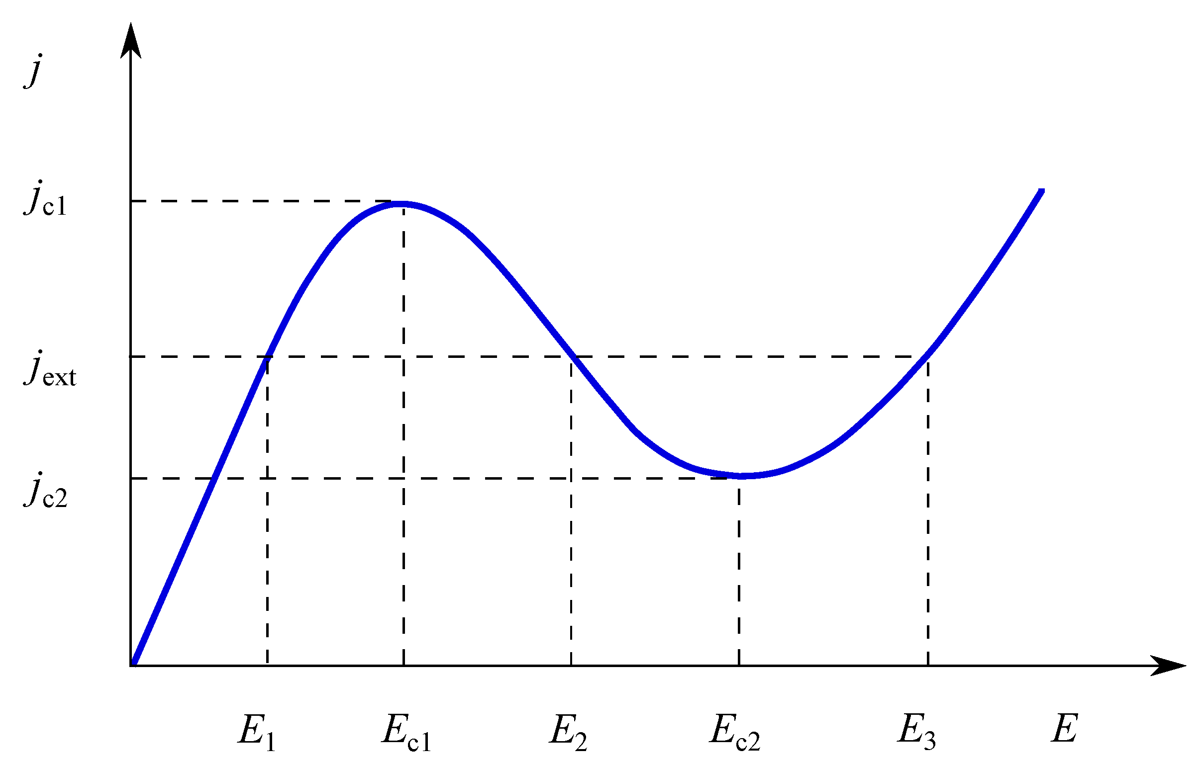
Very briefly, the essence of the phenomenon is as follows. In a strong enough electric field, E, applied to a semiconductor, the conductivity of the sample depends on E, and the current–voltage curve becomes nonlinear. In some cases, calculations based on the assumption of the spatially homogeneous distribution of the current density, j, and E along and across the sample give rise to very unusual behavior of this dependence so that, in a certain area of the E values, an increase in E results in a decrease in j.
In what follows, only one-dimensional cases will be considered, so I can replace
j(
E)
. Then, by definition, the conductivity
. Let us define the differential conductivity as
. Thus, the area mentioned above is characterized with a negative differential conductivity. Here, I will not discuss the microscopic mechanisms explaining the negativeness of
; a detailed description may be found, e.g., in Ref. [
19]. Further increase in
E makes
positive again so that the overall shape of the current–voltage curve resembles letter "
N”, see
Figure 1.
It occurs that the assumption about the spatially uniform distribution of
j and
E in the regions with
is erroneous. This distribution is unstable against small spatially-inhomogeneous perturbations and, eventually, is destroyed owing to their growth. In certain cases, the instability ends up forming a strong field domain bounded by the corresponding layers of charge density. The domain drifts along the sample with a constant speed until it hits the sample edge (anode). The domain disintegrates there, a new one emerges at the opposite side of the sample, and the process repeats. As a result, oscillations with the period
are generated. Here,
L stands for the sample length and
v is the drift speed of the domain. This is the Gunn effect [
9]. It is successfully used in Gunn diodes to generate microwave oscillations [
19].
Let us consider an idealized case of a single traveling strong-field Gunn domain drifting with a constant velocity along an infinitely-large sample. The “strong-field domain” means that the field outside it equals
(see
Figure 1), while inside the domain, it is greater than that. Then, if the voltage applied to the sample is constant, the single domain with a fixed shape is stable, while a configuration with several domains is not. However, if an external source fixes the current in the sample, even the single domain becomes unstable. The instability affects the faces of the domain, which begin to move in opposite directions with respect to the center of the traveling domain. If they move to each other, the domain contracts and, eventually, collapses. If the faces move in the opposite direction, the domain expands and transforms into two traveling layers [
19].
Linear analysis of this secondary instability of a single traveling domain at a fixed current in the circuit was performed by Knight and Peterson [
18]. Mathematically, the stability problem was reduced to the calculation of a gap between the ground and the first excited states in the one-dimensional Schrödinger equation with a complicated potential (see below). To this end, Knight and Peterson employed the Wentzel-Kramers-Brillouin (WKB) approximation. However, this approximation is accurate for highly excited states when the characteristic spatial scale of the wave function oscillations is small relative to the one for the variations of the potential. This is not the case for the ground state. Hence, the accuracy of the results obtained in Ref. [
18] through the WKB method, at least, was questionable. The problem, posed for me by Anisimov, was to check the results of Knight and Peterson employing for the calculations an approximation different from WKB.
If I faced this problem now, quite probably, I would have used the Ritz method supplemented by the orthogonality condition of the wave functions of the ground and excited states [
20]. However, at that time, I was much more ignorant than I am now. Therefore, instead of taking a simple, known way (perhaps, at that time, it was neither simple nor known for me), I decided to go on my own one. Specifically, I decided no less than to find a new method to obtain approximate solutions to the Schrödinger equation opposite to the WKB-method, which could be suitable for the ground and low-excited states. Furthermore, I succeeded in doing that! So, maybe, ignorance is not always bad.
The main idea of the developed approach is somewhat unusual for quantum mechanics, where approximations conventionally are targeted to a wave function, while the potential is given and fixed. However, if one has ground and low-excited states in a complicated potential, the potential has a sharply varying profile relative to that of the wave functions, and the latter is not very sensitive to the fine details of the former. If so, why does one not try to approximate the potential, with some simple shapes, say, with square wells? Then, the Schrödinger equation becomes either exactly solvable or readily treated by perturbation methods.
The most challenging task was to set the first step in this way. The rest was just a matter of not so complicated calculations. I quickly did them and presented the results to Anisimov. “Very well,” he said, “the problem is solved. Write a paper. One more point to be made. Il’ya Mikhailovich Lifshitz has organized a periodic scientific seminar at your Faculty. It takes place every second and fourth Thursday of a month from September to June. I recommend you to contact Il’ya Mikhailovich and ask him to put your talk about this study in the seminar program.”.
Up to now, I remember how difficult it was for me (a fourth-year undergraduate student) to approach such a famous scientist as Il’ya Mikhailovich was and request a talk at his seminar. Finally, I gathered up all my courage and did it. “Excellent,” replied Il’ya Mikhailovich, “Please contact the seminar’s secretary, Mr. Rzhevsky, and ask him to find the nearest free spot in the program. Will 45 minutes be enough for you?”.
To give a 45-min talk in front of an audience of top-rank experts, including a dozen of world-class scientists! My knees turned to jelly, but there was no way to retreat.
It is remarkable that I can vividly remember any moment before and after my talk, but nothing of the talk itself. However, it seems that I stood this test. Moreover, the talk at this seminar was a milestone for my relationship with Il’ya Mikhailovich. Since then, every one of my new results was discussed with him, either through a talk at the seminar or in a private manner at his office at the Kapitza Institute. Later on, I became a close associate and coauthor of Il’ya Mikhailovich [
21]. We even had a joint Ph.D. student. Our close contact lasted until his unexpected premature death of a heart attack in 1982.
However, all this will be later on. At the time I am talking about, I could not imagine even a small part of that.
Thus, the first task (the talk) was complete, but the second remained: I had to write a paper. It was my very first paper, and it took a lot of my time and efforts to do that. Finally, an extended manuscript (in Russian) was submitted to Fizika i Tekhnika Poluprovodnikov (Physics and Technology of Semiconductors).
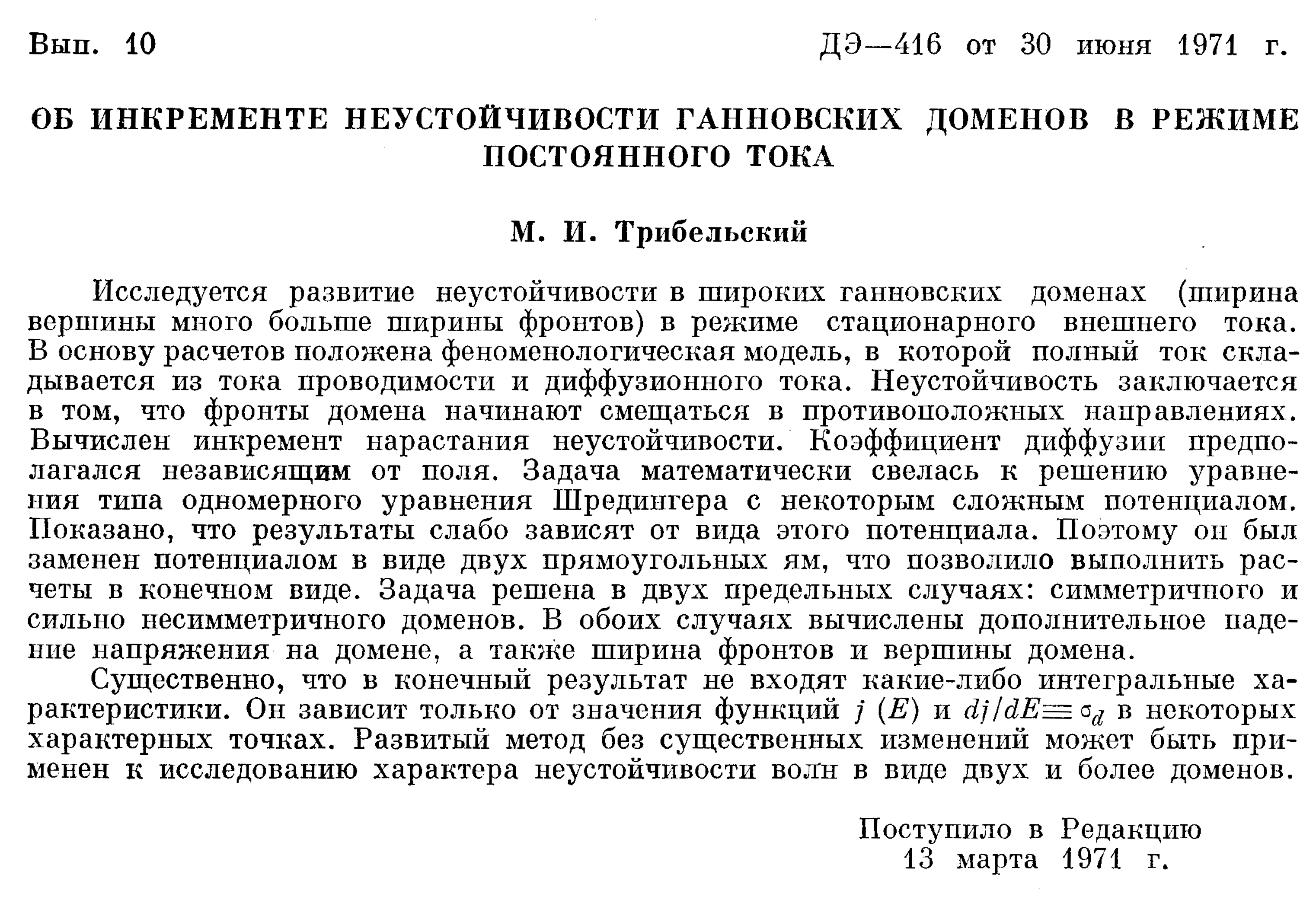
It was the beginning of the bad luck for this paper. At that time, a new publication option was introduced. For some papers (especially lengthy ones), only abstracts were published. The papers themselves were
deposited in specially assigned institutions. If an abstract of such a paper drew somebody’s attention, and he/she was interested in the complete text, a copy of the one could be posted to him/her upon a request. Maybe it was an attempt to reduce the printed size of scientific journals and to solve, at least partly, the eternal Soviet problem of paper deficit. Anyway, my paper was accepted under this condition. Its abstract was published, see
Figure 2, while the full text was deposited at
Research and Development (R&D) Institute Electronics.
Since then, many events have occurred. The country named the Soviet Union does not exist anymore. Regarding
R&D Electronics, I am afraid it has shared the destiny of the country. Now, I am residing within walking distance from the building where
R&D Electronics used to be. It is a shopping mall there. Then, it is quite probable that the full text of my paper has ended up in a nearby scrap-heap, and the abstract reproduced in
Figure 2 is the only remaining piece of the paper.
The English translation reads:
The growth of instability of wide Gunn domains (the width of the top is much larger than the widths of the faces) at the stationary external current regime is inspected. The basis of calculations is the phenomenological model, in which the total current is composed of the conductivity current and the diffusion one. Instability affects the domain faces so that they begin to shift in opposite directions. The instability increment is calculated. The diffusion coefficient is supposed to be independent of the field. Mathematically the stability problem is reduced to a one-dimensional Schrödinger equation with a certain complicated potential. It is shown that the results are weakly dependent on details of this potential. Therefore, the potential is approximated by two square potential wells (separated by a barrier), which made it possible to obtain an explicit expression for the increment. The problem is solved in two limiting cases, namely symmetric and highly asymmetric domains. In both cases, additional drops of voltage on the domain are calculated, as well as the width of the faces and the top of the domain.
It is essential that the final result does not include any integral characteristics of the problem. It depends only on the value of the functions and at certain characteristic points. A developed method without significant changes may be extended to the study of the instability of waves in the form of two or more domains.
The next attempt to publish these results I made after the defense of my Master Science Thesis. An appointed referee of the thesis was another disciple of Landau, Igor Ekhiel’evich Dzyaloshinskii [
22]. After reading the thesis, he said that the results of this level should be available to the international community, and I should publish them abroad in English (when the first draft of the present paper was ready, I learned the sad news: Igor Ekhiel’evich Dzyaloshinskii passed away on 14 July 2021).
To publish abroad, ... it was easier to say than to do. Not to mention poor English, which I had at that time, sending a scientific paper abroad from the Soviet Union was not simple at all. The authors themselves were not eligible to do that. A manuscript had to be sent through specially authorized personnel. The personnel decided whether or not the paper could be submitted abroad, and, if the decision was affirmative, they took care of the submission.
Moreover, prior to the acceptance of the manuscript by the personnel, the authors had to do plenty of paperwork. On top of that, it took 2–3 months on average for mail to be delivered to the addressee. Up to now, I wonder why this was so much. Even if horses delivered the mail; it would not have taken such a long time!
I discussed the matter with Anisimov, and we decided to submit the paper to the East-German journal Physica Status Solidi published in English. There were two reasons for this choice. First, sending a paper to an Eastern bloc country required less paperwork, and chances to get permission for the submission were higher than that in the case of a Western journal. Second, the requirement for the English quality in this journal was not as strict as those in the West. The latter was important since my English was far from being perfect.
Thus, I wrote in English an elaborated version of Ref. [
1] including some new results, did all the required paperwork, gave the bunch of documents to the “authorized personnel,” and... lost control over the submission. Half a year elapsed, but I had not heard anything from the Editors. Then, I sent a postcard to
Physica Status Solidi asking for the status of my paper. A reply came surprisingly fast—in just four months. However, it was pretty unexpected. The Editors informed me that they had never received my manuscript.
By that time, on the one hand, I had already published a paper [
23], where the secondary instability of the Gunn domain was inspected just employing the Ritz method. On the other hand, I got a job and, owing to that, was forced to abandon my study in solid-state physics and focus on an entirely different topic.
Eventually, the results discussed in Ref. [
1] have remained unpublished. Now, fifty years later, I try to realize the advice of Dzyaloshinskii and make these results available to the international community. Perhaps fifty years is a too long period to complete a task, but “that is not lost that comes at last!”.
At the end of these, perhaps lengthy, remarks, I have to say that the results discussed below are not exactly the same as those in Ref. [
1]. First, it is not good to publish the same results twice, even if the fifty years lie between the two publications. Second, I could not do this, even if I wanted to—the original manuscript is lost, and I do not remember all details. Last but not least: now I am a bit more experienced and educated than I was fifty years ago. Therefore, I extracted from this old problem the essential points and generalized them. These points are as follows: (i) the conclusion about the instability of traveling pulses in a broad class of nonlinear diffusion-type problems and (ii) a new method to obtain the bottom-part spectrum of the Schrödinger equation with a complicated potential. A discussion of these two issues is given below.
3. Stability Analysis
The stability analysis performed in Ref. [
18] generalizes a brilliant approach by Zeldovich and Barenblatt for the inspection of the stability of a slow combustion front [
24]. The main idea is as follows. Let us suppose that
, where
is an eigenvalue of the stability problem. If there is a negative
in the problem’s spectrum, it means instability.
Substituting
in Equation (
1) and linearizing the result in small
, one arrives at the eigenvalue problem:
supplemented with the boundary conditions
at
. Then, introducing a new function
connected with
by the relation,
one reduces Equation (
2) to the standard Schrödinger equation:
where
. Let us remark that there is a misprint in the expression for
in Ref. [
19] corrected in Equation (
6).
Note that, since the homoclinic path begins and ends up at the same singular point
and
, the considered steady-state traveling domain solution satisfies the condition
at
. Therefore, as it follows from Equation (
3),
and
, both have the same asymptotic behavior at
. This is important since it means that none of the solutions of the Schrödinger equation generate “false” solutions of the initial stability problem, which may not satisfy the boundary conditions
at
.
Now, the most essential part of the stability analysis begins. If
is a solution of the steady-state version of Equation (
2), then, owing to the translational invariance of the problem
, where
is
any constant, also is its solution, i.e., being substituted in the left-hand side of Equation (
2),
, turns it to zero
identically.
Let us consider the limit . In this case, , and here may be regarded as an infinitesimal perturbation to . The perturbation transforms the steady-state solution into another steady-state solution. This means that such a perturbation is neutrally-stable and should not evolve in time. In other words, it means that is an eigenfunction of the stability problem with zero eigenvalue.
Note that we obtain this result based on the translational invariance solely, without the employment of a specific form of the differential operator in Equation (
2). These neutrally-stable modes generated by a transformation of a continuous group of symmetry are called
Goldstone modes. Since 2008, when the implementation of such a mode in strong-interaction physics (do you remember my remark about interconnections of different fields in physics?) resulted in the Nobel Prize being awarded to Prof. Yoichiro Nambu, they have also been called
Nambu–Goldstone modes.
It is interesting to note that, twenty-five years after the publication of Ref. [
1], I returned to the inspection of the role of Goldstone modes in stability problems. This study resulted in the discovery of a new type of chaos at the onset analogous to the second-order phase transitions in statistical physics, where the mean amplitudes of the turbulent modes played the role of the order parameter [
25,
26,
27].
However, I have departed from the stability analysis of the Gunn domain. It is high time to be back. Actually, not so much remains to be done. Collecting together all mentioned above, one can conclude that
is the eigenfunction of the Schrödinger equation, Equations (
4)–(
6) with zero eigenvalue.
Recall now the oscillation theorem [
20]. The theorem states that, in a one-dimensional Schrödinger equation, the
nth wave function of a discrete spectrum should vanish
n times. Then, it is not a complicated task to show that the integral in the exponent in Equation (
3) always remains finite, i.e.,
never vanishes. Thus, all zeros of
, if any, coincide with those of
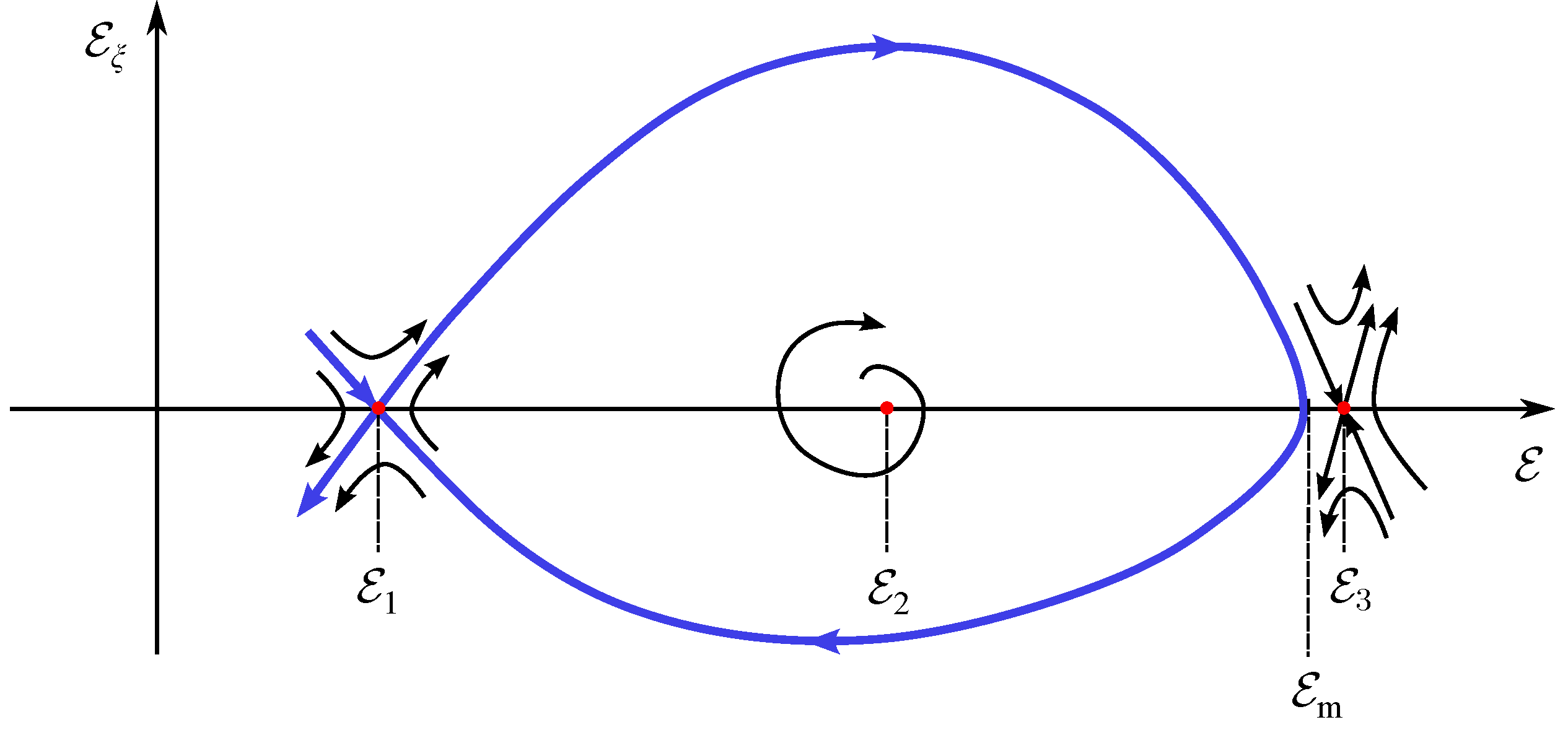
. Finally, since for the traveling domain the profile
has a single maximum (the homoclinic path in the phase plane (
) crosses the
-axis at
, situated in between
and
, see
Figure 3), the product
has a single zero at the value of
corresponding to the maximal field achieved in the domain,
. It means that the wave function (
3) is the one for the first excited state. The “energy” of the ground state should be lower than those for excited states. Since the first excited state has zero “energy” this gives rise to the conclusion that the ground state has negative “energy”, i.e., the spectrum of Equations (
4)–(
6) has a single negative eigenvalue. In other words, the solution
is
unstable with the instability increment equal to the modulus of
, corresponding to the ground state of the Schrödinger equation.
Though the problem in question has several parameters, the actual control parameter, which relatively easily may be varied in an experiment, is the current in the circuit, . Varying , one can change the values of and hence the shape of the traveling domain.
At a certain value of
, the maximal field in the domain,
merges with
, and the homoclinic path in the plane (
) is split into two independent heteroclinic paths connecting the singular points (
) and (
). One of these paths lies entirely in the upper semi-plane. For this solution,
is always positive at any finite
. The other lies entirely in the lower semi-plane and, for it,
at any finite
, see
Figure 3. Each of these solutions corresponds to a traveling charge layer transferring the sample from one steady-state to another steady-state.
It is important that, since, for the layers,
does not vanish at any finite
, the corresponding wave function given by Equation (
7) is the one of the
ground state of the Schrödinger equation. This means that, in contrast to the traveling domain, the traveling layers are
stable [
18,
19].
4. Spectrum of Schrödinger Equation
Thus, to get the value of the instability increment and, hence, the characteristic time for the traveling domain decomposition, one has to obtain the energy level for the ground state in the Schrödinger equation with the complicated potential given by Equation (
6). As it has been mentioned above, the main idea employed in Ref. [
1] to fulfill this task is to approximate the actual smooth potential by a superposition of square potential wells. The parameters of the wells are selected so that the approximated potential keeps all main features of the initial smooth profile. One of the approximation parameters remains free. It is fixed by the condition that, for the first excited state,
.
This procedure reduces the solution of the complicated initial problem to finding the roots of a set of transcendental equations. In the worst case, the latter may be readily done numerically. To illustrate this rather general approach, a simple case of a broad traveling domain is discussed below.
The domain becomes broad when
approaches
. In the phase plane, it corresponds to the shift of the regular point of the path (
) toward the saddle (
). In this case, the domain approximately may be presented as a nonlinear superposition of two layers with opposite charges, and the potential (
6) has a shape of two wells separated by a barrier.
Each well is associated with the corresponding layer. The width of the barrier equals the distance between the layers and is large in the case under consideration. Then, the tunneling through the barrier is exponentially weak. If the tunneling were suppressed entirely, each well would have corresponded to the potential generated by a single layer and, in accordance with the mentioned above, had the ground state with . Thus, it is clear that the level with for the domain occurs due to the finite tunneling resulting in the splitting of the ground states in the two wells with the same value of . Therefore, instead of the employment of a rather cumbersome general procedure of the solution of an entire problem with the finite tunneling, let us, first, neglect the tunneling and consider the solutions of the Schrödinger equation in each square well separately. Then, the finite tunneling is taken into account with the help of perturbation theory.
The values of the parameters of the square wells approximating the smooth profile of the potential may be obtained by inspection of Equation (
6). For example, bearing in mind that at
, the solution
describing the domain satisfies the conditions
;
and that, by definition,
, one immediately obtains that both outer walls of the wells have a height equal to
. Similarly, the barrier height is
. The widths of the wells and the barrier are estimated based on the exact solution describing the domain path in the phase plane obtained in Ref. [
18]. The last remaining parameters are the depths of the wells. They are fixed by the conditions that the ground state in each well has
.
I do not present here these simple but cumbersome calculations. Just note that the problem is rather robust against errors in the approximation of . The robustness is related to the smallness of the split of the ground levels in the wells due to the tunneling and the fact that, at the employed approach, the important condition for the ground state in each separate well holds automatically.
Let us suppose that the wave functions,
, of the ground state for each well are known and that these wave functions satisfy the equations
. Here,
designates the Hamiltonians, whose potentials,
are the corresponding single-well potentials. Let us look for the wave function of the complete problem with the two-well potential in a form of a linear superposition of
:
where
are constants, which should be defined in the course of calculations. Then, since
is an eigenfunction of the complete Hamiltonian
,
Making scalar products with
and taking into account the normalization conditions
, one arrives from Equation (
9) to the following equations for
:
where
and
stand for the corresponding matrix elements. Note that the wave functions
and
are
not orthogonal since they are the eigenfunctions of the
different Hamiltonians, namely,
and
.
The solvability condition requires vanishing of the determinant of Equations (
10) and (
11). This results in a quadratic equation for
. The difference,
, between the two roots of this equation approximately equals the desired instability increment.
This result has completed the instability analysis. However, the exact expression for
is rather cumbersome. Therefore, it is worth simplifying this result, employing the smallness of certain parameters in Equations (
10) and (
11). To this end, I have to estimate the matrix elements and the overlap integrals
.
To calculate the matrix elements, it is convenient to single out from the full double-well square potential,
, the part corresponding to a single well, i.e., to suppose that
, see
Figure 4, where for the first well (left side of
Figure 4),
at
, while, at
, the sum of
and
equals the height of the barrier. Similarly, for the second well (right), the sum
equals the height of the barrier at
, while, at
, the potential
. Thus,
are the single-well potentials, and the corresponding Hamiltonians acting on their wave functions produce zero. Then, the leading terms in the matrix elements are estimated as follows:
where
is the barrier width. The same estimate is true for
(for the sake of simplicity, the widths of the corresponding wells,
, are supposed to be not small). In the same manner, one obtains
Then, in the leading approximation,
Thus, as it could be expected, the value of the instability increment for the broad domain is exponentially small indeed.
Finally, note that, for each single square well, the normalized wave functions
may be readily obtained in the explicit form, including the normalization constant. Then, it is just a matter of more or less routine calculations to improve the accuracy of Equation (
14), taking into account the prefactors and dropped higher-order exponentially small terms.


