Yang–Mills Theory of Gravity


Department of Mathematical Science, Ritsumeikan University, 4-2-28, Kusatsu-Shi, Shiga 525-0034, Japan
Physics 2019, 1(3), 339-359; https://doi.org/10.3390/physics1030025
Submission received: 25 June 2019
/
Revised: 15 October 2019
/
Accepted: 22 October 2019
/
Published: 12 November 2019
(This article belongs to the Section Classical Physics)
Abstract
The canonical formulation of general relativity (GR) is based on decomposition space–time manifold M into , where R represents the time, and Σ is the three-dimensional space-like surface. This decomposition has to preserve the invariance of GR, invariance under general coordinates, and local Lorentz transformations. These symmetries are associated with conserved currents that are coupled to gravity. These symmetries are studied on a three dimensional space-like hypersurface embedded in a four-dimensional space–time manifold. This implies continuous symmetries and conserved currents by Noether’s theorem on that surface. We construct a three-form (D represents covariant exterior derivative) in the phase space on the surface , and derive an equation of continuity on that surface, and search for canonical relations and a Lagrangian that correspond to the same equation of continuity according to the canonical field theory. We find that is a conjugate momentum of and is its energy density. We show that there is conserved spin current that couples to , and show that we have to include the term in GR. Lagrangian, where , and is complex connection. The term includes one variable, , similar to Yang–Mills gauge theory. Finally we couple the connection to a left-handed spinor field , and find the corresponding beta function.
1. Introduction
Gravity can be formulated based on gauge theory by gauging the Lorentz group [1]. For this purpose, we need to fix some base space and consider that the Lorentz group acts locally on Lorentz frames which are regarded as a frame bundle over a fixed base space. We can consider this base space as an arbitrary space–time manifold M with coordinates , and consider the local Lorentz frame as an element in the tangent frame bundle over M. By that we have two symmetries; invariance under continuous transformations of local Lorentz frame, group, and invariance under diffeomorphism of the space–time M, which is originally considered as a base space [2].
Since the group is a subgroup of , the Lagrangian of gravity has an internal gauge symmetry group . Thus the elements of act locally on some spacial Lorentz orthonormal frames , we consider these frames as a basis of the tangent vector bundle on the three-dimensional space-like hypersurface . Using some local coordinate system , on , we expand these basis vectors into , so defining the gravitational field with metric on . Using the isomorphism between Lie algebra of and that of , one can regard also as a local -valued one-form. So we have an vector bundle with real spin connection [3]. These facts can be generated into self-dual and anti-self-dual formalism of general relativity (GR) with complex connection and complex conjugate one-form field .
This paper proceeds as follows: We start with the four-dimensional (4D) Palatini Lagrangian and perform a decomposition based on the decomposition , where R represents the time, and is the three-dimensional (3D) space-like surface, thus we specify the Lagrangian part on . Then we try to show that is independent of time on this surface, we try to prove this fact using the fact that there are no dynamics in the space-like region of M. After that we use to get an equation of continuity on , and search for canonical relations and Lagrangian that correspond to the same equation of continuity according to the canonical field theory. We find that is a conjugate momentum of and is its energy density. We obtain a Lagrangian for the connection in 4-manifold M, then we couple it to a left-handed fermion field and find the beta function.
2. Decomposition Space–Time Manifold M into
The formulation of GR based on decomposition space–time manifold M into is needed for expressing the metric of space–time as a solution of an equation for time evolution, such as in the Hamiltonian formulation. Thus the time evolution is the changing of the geometry of this surface. This decomposition preserves the continuous symmetries (gauge invariance and diffeomorphism invariance) of GR and its canonical quantization, so we can use it for the gauge theory of GR [4,5,6,7].
We define gravitational field as a one-form that is related with metric on an arbitrary space–time manifold M by , with spin connection , where is Lie algebra of Lorentz group . The spin connection defines covariant derivative that acts on all fields which have Lorentz indices :
We start with the GR Lagrangian of the form
where
is the Riemannian curvature tensor and satisfies .
By the decomposition , we decompose this Lagrangian into
where i and j are Lorentz indices for , and . The part
has the gauge symmetry of the group , which is a subgroup of , it also relates to the geometry of the surface under the variation in the direction of subject to , , since it depends only on the metric which is defined on , which is intrinsic geometry.
Since is an anti-symmetric tensor, we can introduce a new one-form field , the Hodge dual of in the internal spin space on the surface ; , it is called the gravitational electric field [8,9]
For example .
For the Lagrangian part on , we use the first one:
The remaining part
associates with the time evolution under the variation in the normal direction of , it is subject to , , and changes the geometry of the surface during the time. Dynamics, such as propagation in the time-like region , and determines how the surface is embedded into the manifold M, which is extrinsic geometry. But the surface is embedded in a space-like region in M; , so there are no dynamics on . We can see this fact by noting that (the covariant derivative of the metric is zero), so
We will rewrite as , for . The formula is more general than since there is , and so its projection onto is zero. This case appears in the diffeomorphism maps of into another space-like surface, as we will see.
We can study the embedding of by letting the time derivative of a position vector on its tangent space be in the direction of the normal to this tangent space . We can see this by considering a position vector that satisfies . Let , where is the normal space to , and is a covariant derivative of with respect to the time . From , we obtain , so . Since , we have , thus we get which means that the points of M do not expand nor contract covariantly in the space-like , but is possible.
Therefore, for a diffeomorphism map of into another space-like surface (consider this as time evolution), it must be
and
This means for each , the covariant propagation does not occur in , but it occurs in
This is a changing in the embedding of in M. Let satisfy , where is matrix notation and n is the normal to . This normal is in the direction of the time, so it carries one index; , thus . It must also satisfy , so . Using this in , we obtain , so we get . Thus we get , and by , we obtain . This formula is for determining .
Let us suggest a formula for determining like
where , and is the full metric. Let us write using matrix notation , its elements are . Let satisfy . Thus we get the inversion
this is obtaining the metric component from ; the changing of the metric with respect to the time. Thus if we fix the metric component , like , we obtain the map . So we have an immersion . In another words, for an immersion , and under some hypotheses, we can construct a metric on using the metric on . Our hypothesis here is .
First we find the matrices then . The matrices are symmetric and satisfy , where the vector is the unit vector in , we can write them in a simple form like
the angles and can be determined to satisfy , thus we obtain
Therefore the matrices can be written in the form
the constants and are determined to satisfy
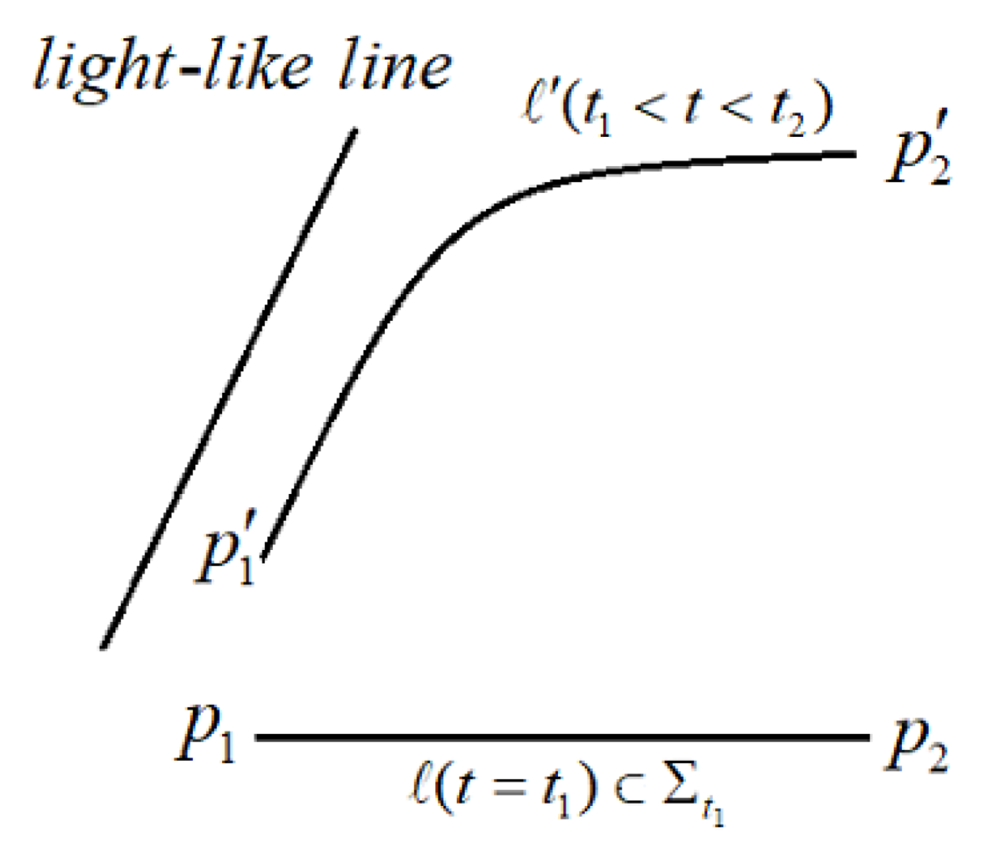
We can consider that as a continuous changing in the embedding of in M;which is a diffeomorphism map. Since the Lagrangian depends only on while the term depends on , thus by the previous discussing we have a map (time evolution), with . As illustrated in the following Figure 1.
Let which propagated to , both surfaces are space-like, but the trajectories of the propagation and lie in the time-like region. The length of ℓ is also increased. Thus, this means that the metric mapped to metric by Equation (6), which means the length is given by
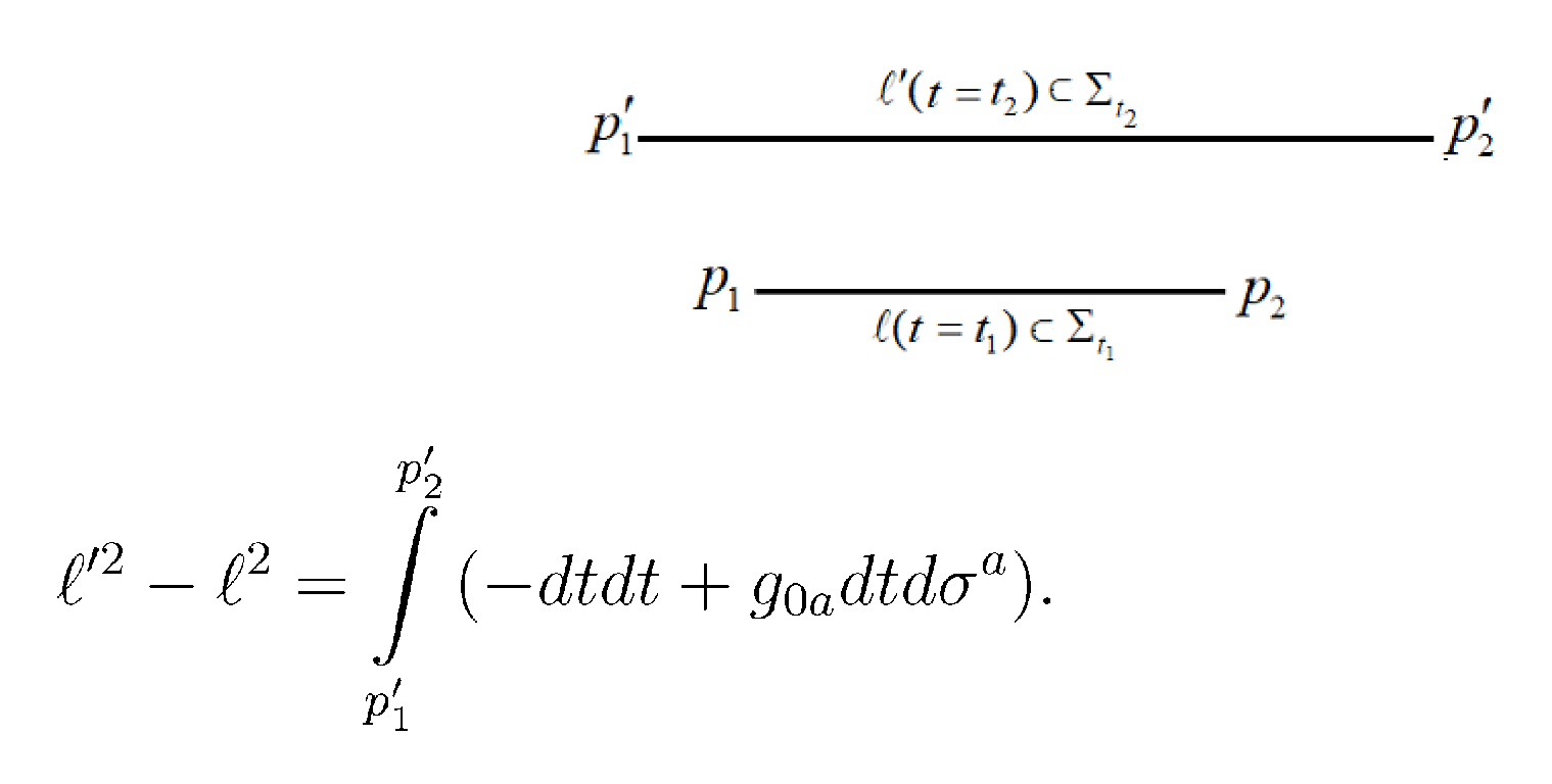
which again can be mapped into a space-like surface by an isometric map such . which results in Figure 2:
The limit corresponds to and , not to (with and ). For example, if two particles and exchange photons with wavelength in , then in they measure a different wavelength, namely . The difference is given by , where we set . Thus the two particles and measure after a time the difference , where is given in Equation (6).
Thus we study the embedding of surface and its changing in manifold M using the metric on and its derivative with respect to the time.
The Lagrangian is a function on the space-like space , therefore, it is independent of time, on . We can see this by using the fact
we have
which is a function on , not on ; which means there are no dynamics on the space-like region .
Let us write , where is a projection of onto a surface , the inner product of V with tangent basis in , defined below in Equation (17), and is three-form in the phase space on . Thus we write
If we write as
with and , we obtain
Since is three-form on , so , if we add it to the last formula, we get
This relates the Lagrangian and with this surface. Under arbitrary transformation , the two Lagrangian parts and will mix. Thus and the basis on transforms as
Therefore, the components of three-form transforms as
To keep the invariance under this transformation, that is still holds, we write the three-form in the phase space on M, and let be its projection onto . Therefore we write
thus we get three-form in the phase space on M, it has internal symmetry. Its projection onto is
We write using self-dual formalism (Plebanski formalism) [11] in which the connection is a three-complex one-form given by
where is self-dual projector given by Equation (3). The curvature which associates with this connection is
On the surface , it is
Also
Thus we have self-dual plus anti-self-dual projection:
where and are the Hermitian conjugate of and . This projection relates to the decomposition of Lie algebra of the Lorentz group into two copies of Lie algebra of [12].
We write the components of the curvature as
where
which motivates introducing a notation of the covariant derivative like [7]
or
so
where the matrix elements are the elements of the generators in the adjoint representation of the group [13]. The coupling constant here is . In general we write this covariant derivative as
Using the projection in Equation (12), we rewrite in the complex phase space as
where we take in consideration only the first part, the second is obtained by taking the Hermitian conjugate. We can write it as three-form on M as done in Equation (9), we obtain
Its projection onto is
where is complex connection, and is a complex one-form as defined in Equation (11).
3. Equation of Continuity on the Hypersurface
We have showed that the Lagrangian is independent of time, on since . This relates to the fact that there are no dynamics in the space-like ; the points of M do not expand nor contract covariantly in this region, . Note that although , but it may be . We had
which shows that the two parts of the Lagrangian and mix by time evolution. Then we wrote as , where is three-form in the phase space on M (Equation (7)), its projection onto is Equation (17)
In self-dual formalism, we obtained , with
Our condition makes sense here because of the decomposition and fixing a coordinate system on the hypersurface , this yields to an equation of continuity on this surface. For this purpose, we take the inner product of the four-form with a tangent basis on the surface at an arbitrary point, we get a one-form co-vector in the direction of the normal to this surface at that point. Then we set , we obtain an equation of continuity on .
Now taking the exterior derivative of Equation (15), we obtain
where . The tri-tangent basic on is , we rewrite it as . The projection of onto this basic is
where is contraction pairing defined by
where the bracket is anti-symmetrization of the indices. Although is zero in manifold M, but the contraction pairing of with basis is not zero as we will see, since we do not sum over the time index as we sum over the spatial indices , because we regard as normal to the surface .
For cotangent basis and tangent basis , this pairing can be defined simply by using inner product like [14]
in which we consider for , so regarding to our gauge.
Starting with the first term
we get
The second term is
Doing the same thing, we get
Adding the two terms, we obtain
Its Hodge dual on the surface with respect to the coordinates is
Also we define the complex two-form field from Equation (3) as
Using them in the last formula, we get
And using
we obtain
With
it becomes
As we suggested before, we let the normal of the surface be in direction of the time , so is in direction of the time. Therefore we set , thus we get
The vector is one-form in the direction of the normal to the surface . It is zero as we mentioned before, thus we get
or
We write it as
The term is scalar, so , the vector is a usual vector field on , it does not carry a Lorentz index, so and , thus we get
using
This equation shows that there is a relation between and in the space on manifold . Usually this relation is written as . We can find that relation by regarding this equation as an equation of continuity with respect to a Lagrangian like that satisfies the action principle and the invariance under continuous symmetries of GR. Therefore we regard as energy density , and as momentum density , where c is constant for satisfying the units. Then we search for a suitable Lagrangian and Hamiltonian with canonical relations that correspond to the same continuity equation according to the quantum fields theory, we do this at the flat-space–time limit and generalize it to an arbitrary curved space–time.
In scalar field theory, the Lagrangian is [15]
the conjugate momentum is . The conserved momentum–energy tensor is
In the flat limit of the space–time, our momentum–energy tensor is
and
comparing it with the momentum , we conclude that our conjugate momentum is [16,17,18,19].
By considering a Lagrangian of the form with corresponding Hamiltonian like and using the action principle and the diffeomorphism invariance on the surface , we obtain the momentum–energy tensor like [16,17,18]
Comparing them with our momentum–energy tensor and , we conclude
Using Equation (22) in Equation (21), we get
therefore we set , so , and , we obtain
which means that is conjugate momentum of . Using it in the Hamiltonian :
then using our energy density , we get the Lagrangian
Therefore
so
where and are defined in Equations (3) and (18). This Lagrangian has a symmetry of the complex group and the self-dual of Lorentz group . The contraction is defined by using the metric . This Lagrangian corresponds to self-dual part of Equation (12). To get the total Lagrangian, we add the Hermitian conjugate, we obtain :
the curvature is the Hermitian conjugate (10). The Lorentz group is , its Lie algebra is reducible and can be decomposed into two copies of the Lie algebra of : .
The complex connection takes values in Lie algebra of , while its Hermitian conjugate takes values in Lie algebra of . Thus the Lorentz invariance is satisfied by the uni-variance under the two groups and [11,12].
To determine the constant c, we write this Lagrangian in the form
by using properties of the projection
the Lagrangian (Equation (25)) becomes , thus . Therefore
this Lagrangian is similar to the Plebanisky Lagrangian, but it is not multiplied by the imaginary number i and does not include the cosmological constant term.
4. Yang–Mills Theory of Gravity
By regarding the local Lorentz symmetry as a gauge symmetry with spin connection (or ) as gauge fields, we recognize Yang–Mills theory in gravity. But not full gravity, since in the Yang–Mills theory, the variables are connections and conserved currents, while in the gravity the metric is also variable. The local Lorentz symmetry generates locally conserved currents, and those currents are coupled to spin connection . This makes the local Lorentz symmetry a gauge symmetry with the Lorentz group as a gauge group. Also, these currents must be conserved and vanish in the vacuum.
From the formula , we can get the inversion by inserting it back, we obtain
We can get the equation of motion from this Lagrangian (Equation (27)) by adding terms like
therefore the and yields and . But by using properties of the self-dual projection from Equation (26), we obtain and , but this does not change the equations of motion.
But as we will see, if there is a Lorentz current, like the spin current of the spinor field, then , therefore to keep , and to also keep , we add a term like . This is done in order to insert back in into the Lagrangian. Therefore we write
where k is a constant can relate to a coupling constant of Lorentz current with the spin connection .
This Lagrangian includes , is given in Equation (18), similarly to Lagrangian in Yang–Mills theory with gauge group , and the self-dual of Lorentz group . It depends only on the connection , thus it describes the changing of the local Lorentz basis. Therefore reads the invariance only under the local Lorentz transformations. Also, it is a topological invariance, so it allows the free propagation of spin connection . But by relating with the triad , and relating with the metric by , this breaks the free propagation of spin connection as free waves, except in the background approximation of the metric, the result is gravitational waves. Similarly to the free electromagnetic field.
By using the properties of self-dual projection, this Lagrangian can be written using the Riemannian tensor as
We find the role of the term by including the interaction of mass-less spinor particles with gravity. Since they are massless, their energies are small so that their interaction with the gravitational field is weak, but their interaction with spin connection takes place. The interaction term is
where is Lorentz current. If we add this term to the Lagrangian
we get
So the equation of motion for is
In self-dual formalism, this equation becomes
These two equations say that the Lorentz current is the source for the gravitational field , but this is not right since the energy is the source for it, also we choose . Thus, these equations do not hold. But if we use the Lagrangian
the equation of motion for becomes
Thus we choose and
The term includes only the spin connection , so the Lorentz current contributes as a source for the spin connection , and so interacts with it. This relate to the fact that we can regard the local Lorentz symmetry as a gauge group with spin connection (or ) as gauge fields. The Lorentz current is conserved since
Furthermore, Equation (30) allows us to calculate a Lorentz current for a given curvature , although the curvatures and are calculated using only the energy–momentum tensor. Although there are Lorentz currents associated with matter, those currents relate to the local Lorentz symmetry.
We need to prove in the vacuum, where is Riemann curvature tensor, it satisfies , and . In the vacuum, we have the equality
where is a Ricci tensor and . This equality is equivalent to another equality [11]:
with Hodge operator
the anti-symmetric tensor is the volume four-form for metric . Therefore in the vacuum, we have
acting by on both sides, with we get
The summing here is over and , while and are fixed. Then multiplying both sides by :
We note that by summing over in for each fixed , we obtain the Bianchi identity , therefore
It becomes
so in the vacuum. Therefore the Lorentz current vanish in the vacuum. Using the self-dual projection, we find
also vanish in the vacuum. Therefore this current associates only with matter. We can also prove this by using the formula , and by setting in the vacuum [11]. Using
with , and
Hodge operator here is with respect to the metric , we get
The first term becomes
and by Bianchi identity , we obtain . Therefore
Since in the vacuum, we get .
Therefore for a Lorentz current that associates with matter, we get
where we used and , with property of Hodge dual twice operation on p-form V in n dimensions: , where , and t is the number of negative eigenvalues of the metric tensor [14]. In our case we have .
Same thing we get for , (Equation (32)):
Therefore
so
The quantity depends on the triads , and on spin connection , while relates matter. Therefore by solving this equation for a given Lorentz current , we get solutions for and . But this formula reads only the contributing of Lorentz current in , there is a contributing of cosmological constant and matter in symmetric part of ; , where T is trace of energy-momentum tensor [12,22]. Since Lorentz current generates local Lorentz transformation, we expect that in Equation (33) is anti-symmetric, this distinguishes contributing of from those of cosmological constant and matter. So we write
thus contributes in anti-symmetric part of , where is vector field in local Lorentz frame.
Let us write , with Lorentz current defined in Equation (28). The relationship (linear) between and can be determined by inserting in Equation (34). It is easier to solve
in region away from matter where , so we can solve it in background approximation, , thus in spherically coordinates. If we assume that the vector field depends only on the radius r, we get
where is constant vector. Therefore the contributing of Lorentz current in the curvature is
therefore the contributing of in is
This formula satisfies , it is similar to electric field . This is similarity between GR and Yang-Mills theory.
The Lorentz current is not associated only with spinor particles, the Lorentz symmetry for arbitrary field produces a global conserved Lorentz current like ([15], section 22)
is energy-momentum tensor in flat space–time. Locally we write this as
where is constant, therefore
The existence of a conserved spin current that couples to lets us to believe in local Lorentz symmetry as a gauge group with spin connection (or ) as gauge fields similarly to Yang–Mills theory.
5. Beta Function
We assume that the interaction of mass-less particles with the gravity is dominated by interaction of their spin current (Lorentz current) with the connection . We can use the Lagrangian to describe the interaction of left-handed fermions with the connection . We choose a representation of in which we have , where are boost generators and are rotation generators [23]. Our connection is a one-form complex given by the self-dual projection of the spin connection according to the decomposition [24]. Therefore
or , where and are real.
For simplicity let us choose , with a constant . Thus the connection becomes
with new generators .
Therefore the coupling of the connection with left-handed spinor field is , where g is coupling constants comes from using the covariant derivative seen in Equation (14). So we write the fermion-gravity Lagrangian as
Using the metric , we obtain
In background space–time, we have , so , where is the Minkowski metric. Therefore the gravity and spinor Lagrangian approximates to
The remaining term includes the interaction with the fluctuated gravitational field , this interaction relates with local invariance under diffeomorphism of M. Let us consider only the part
which is invariant under local Lorentz transformation, the compatible currents take values in , thus is coupled to Lorentz currents. By that we have included only the invariance under local Lorentz transformation and excluded the local invariance under diffeomorphism of M. Thus we describe the GR using Lorentz frames as vector bundle over basis space M with connection .
It is similar to the Lagrangian of Yang–Mills theory for spinor field, but with the generators , so to get results from the usual theory, we just replace the generators with . For example, to get the beta function for our Lagrangian, we use the beta function of Yang–Mills theory for spinor field with symmetry group like , it is given by [15,25]
The numbers and , are given in
where are generators for the fundamental representation of and are generators for the adjoint representation. To get them for our Lagrangian, we have to start with the commutation relation and note that we can multiply both sides by to get
thus we get new anti-symmetric structure constants , although the new generators are not hermitian, but this does not violates the methods of deriving the beta function, the necessary thing in deriving it is keeping , and constants [15,26,27]. Anyway, we will absorb the modification factor into the coupling constant g, so we have gauge group with complex coupling constant like . Therefore we obtain
and
Thus to get beta function for our Lagrangian, we replace with and with , so using this in the beta function
we get
For the group , we have and , so for , we obtain beta function like
Taking in consideration the first statement we obtain
which can be solved for energy scale M as
Usually the coupling constant is real, so for our one, we consider that the interaction strength is governed by the real part of the coupling constant g, this is
thus the behavior of interaction of the left-fermions with the spin connection according to our Lagrangian depends on , if , then , which means that this interaction becomes stronger as the energy increases, until breaking the perturbation at some energy scale. It is natural to consider since we expect in nature; the gravity effects the particles by changing their energies (like accelerating a particle via a gravitational field) not by changing their angular momentums. So from , we have for this case.
But when does the case appear? it appears when , in this case, the gravity induces a rotation of the inertial frame (the Lorentz frame moves with a particle, or the Lorentz frame in which the particle has a constant speed) more than changing the energy of that particle (accelerating). This occurs when there is the smallest distance between two particles which interact by their gravitational field. At this distance, the velocities of the two particles are constant, so the interaction by the gravity is dominated by changing their angular momentum, thus so . This situation appears in the back holes; which is a confinement of .
6. Conclusions
We have considered the spacial Lorentz orthonormal basis as an element in a vector bundle with real spin connection , which takes values in the Lie algebra of group or . We considered this vector bundle as a tangent vector bundle on the hypersurface of constant time , this allowed us to define three-form in the phase space on this surface. By arbitrary transformation of , the three-form becomes on M, but is always satisfied. By doing the same thing, we obtained the equation using self-dual and anti-self-dual formalism. This equation produces an equation of continuity on the hypersurface . We found that is a conjugate momentum of where is its energy density. We saw that we have to include the term in the GR Lagrangian, since there is a conserved spin current that couples to . This is the similarity between GR and Yang–Mills theory of gauge fields. If we can solve the GR equations using only spin current, we may consider GR as Yang–Mills theory of gauge fields on a curved space–time manifold with spin connection as a gauge field.
Conflicts of Interest
The authors declare no conflict of interest.
References
- Montesinos, M.; González, D.; Celada, M.; íaz, B. Reformulation of the symmetries of first-order general relativity. Class. Quant. Grav. 2017, 34, 205002. [Google Scholar] [CrossRef]
- Weatherall, J.O. Fiber Bundles, Yang–Mills Theory, and General Relativity. Synthese 2016, 193, 2389. [Google Scholar] [CrossRef]
- Fleischhack, C. On Ashtekar’s Formulation of General Relativity. J. Phys. Conf. Ser. 2012, 360, 012022. [Google Scholar] [CrossRef]
- Arnowitt, R.; Deser, S.; Misner, C.W. The Dynamics of General Relativity. Gen Relat. Grav. 2008, 40, 1997–2027. [Google Scholar] [CrossRef]
- Wald, R.M. General Relativity; University of Chicago Press: Chicago, IL, USA, 1984; ISBN-13: 978-0226870335. [Google Scholar]
- Ponomarev, V.N.; Barvinsky, A.O.; Obukhov, Y.N. Gauge Approach and Quantization Methods in Gravity Theory; Nauka: Moscow, Russia, 2017; ISBN 978-5-02-040047-4. [Google Scholar] [CrossRef]
- Rosas-Rodriguez, R. Alternative variables for the dynamics of general relativity. Int. J. Mod. Phys. A 2008, 23, 895–908. [Google Scholar] [CrossRef]
- Rovelli, C. Ashtekar formulation of general relativity and loop-space nonperturbative quantum gravity: A report. Class. Quantum Grav. 1991, 8, 1613. [Google Scholar] [CrossRef]
- Rovelli, C. Area is the length of Ashtekar’s triad field. Phys. Rev. D 2013, 87, 089902. [Google Scholar] [CrossRef]
- Rovelli, C. Quantum Gravity; Cambridge University Press: Cambridge, UK, 2004; ISBN 978-0521715966. [Google Scholar]
- Krasnov, K. Plebański formulation of general relativity: A practical introduction. Gen. Relat. Grav. 2011, 43, 1. [Google Scholar] [CrossRef]
- Bennett, D.L.; Laperashvili, L.V.; Nielsen, H.B.; Tureanu, A. Gravity and Mirror Gravity in Plebanski Formulation. Int. J. Mod. Phys. A 2013, 28, 1350035. [Google Scholar] [CrossRef]
- Georgi, H. Lie Algebras in Particle Physics; CRC Press, Taylor & Francis Group: Boca Raton, FL, USA, 2000; ISBN 9780429499210. [Google Scholar] [CrossRef]
- Pope, C. Geometry and Group Theory; Texas A&M University Press: College Station, TX, USA, 2008. [Google Scholar]
- Srednicki, M. Quantum Field Theory; Cambridge University Press: Cambridge, UK, 2007; ISBN 9780521864497. [Google Scholar]
- Struckmeier, J.; Redelbach, A. Covariant Hamiltonian field theory. Int. J. Mod. Phys. E 2008, 17, 435–491. [Google Scholar] [CrossRef]
- Zambrano, G.E.; Pimentel, B.M. Canonical structure of gauge invariance proca’s electrodynamics theory. Momento 2018, 56, 26–44. [Google Scholar] [CrossRef]
- Creutz, M.; Muzinich, I.J.; Tudron, T.N. Gauge fixing and canonical quantization. Phys. Rev. D 1979, 19, 531. [Google Scholar] [CrossRef]
- Utiyama, R. Invariant Theoretical Interpretation of Interaction. Phys. Rev. 1956, 101, 1597. [Google Scholar] [CrossRef]
- Engle, J.; Noui, K.; Perez, A.; Pranzetti, D. Black hole entropy from an SU(2)-invariant formulation of Type I isolated horizons. Phys. Rev. D 2010, 82, 044050. [Google Scholar] [CrossRef]
- Engle, J.; Noui, K.; Perez, A. Black hole entropy and SU(2) Chern-Simons theory. Phys. Rev. Lett. 2010, 105, 031302. [Google Scholar] [CrossRef] [PubMed]
- Tennie, F.; Wohlfarth, M.N.R. Consistent matter couplings for Plebanski gravity. Phys. Rev. D 2010, 28, 104052. [Google Scholar] [CrossRef]
- Başkal, S.; Kim, Y.; Noz, M. Loop Representation of Wigner’s Little Groups. Symmetry 2017, 9, 97. [Google Scholar] [CrossRef]
- Herfray, Y. Pure Connection Formulation, Twistors and the Chase for a Twistor Action for General Relativity. J. Math. Phys. 2017, 58, 112505. [Google Scholar] [CrossRef]
- Herzog, F.; Ruijl, B.; Ueda, T.; Vermaseren, J.A.M.; Vogt, A. The five-loop beta function of Yang–Mills theory with fermions. JHEP 2017, 1702, 90. [Google Scholar] [CrossRef]
- Cui, J.W.; Wu, Y.L. One-Loop Renormalization of Non-Abelian Gauge Theory and beta Function Based on Loop Regularization Method. Int. J. Mod. Phys. A 2008, 23, 2861–2913. [Google Scholar] [CrossRef]
- Peskin, M.E.; Schroeder, D.V. An Introduction to Quantum Field Theory; Westview Press: Boulder, CO, USA, 1995; ISBN 9780201503975. [Google Scholar]
Figure 1.
Propagation of space-like surface.

Figure 2.
Changing distance between two space-like points after propagation.

© 2019 by the author. Licensee MDPI, Basel, Switzerland. This article is an open access article distributed under the terms and conditions of the Creative Commons Attribution (CC BY) license (http://creativecommons.org/licenses/by/4.0/).
Share and Cite
MDPI and ACS Style
Matwi, M.A. Yang–Mills Theory of Gravity. Physics 2019, 1, 339-359. https://doi.org/10.3390/physics1030025
AMA Style
Matwi MA. Yang–Mills Theory of Gravity. Physics. 2019; 1(3):339-359. https://doi.org/10.3390/physics1030025
Chicago/Turabian StyleMatwi, Malik Al. 2019. "Yang–Mills Theory of Gravity" Physics 1, no. 3: 339-359. https://doi.org/10.3390/physics1030025
APA StyleMatwi, M. A. (2019). Yang–Mills Theory of Gravity. Physics, 1(3), 339-359. https://doi.org/10.3390/physics1030025