All articles published by MDPI are made immediately available worldwide under an open access license. No special
permission is required to reuse all or part of the article published by MDPI, including figures and tables. For
articles published under an open access Creative Common CC BY license, any part of the article may be reused without
permission provided that the original article is clearly cited. For more information, please refer to
https://www.mdpi.com/openaccess.
Feature papers represent the most advanced research with significant potential for high impact in the field. A Feature
Paper should be a substantial original Article that involves several techniques or approaches, provides an outlook for
future research directions and describes possible research applications.
Feature papers are submitted upon individual invitation or recommendation by the scientific editors and must receive
positive feedback from the reviewers.
Editor’s Choice articles are based on recommendations by the scientific editors of MDPI journals from around the world.
Editors select a small number of articles recently published in the journal that they believe will be particularly
interesting to readers, or important in the respective research area. The aim is to provide a snapshot of some of the
most exciting work published in the various research areas of the journal.
The question of constructing models for the evolution of clusters that differ in shape based on the Boltzmann’s H-theorem is investigated. The first, simplest kinetic equations are proposed and their properties are studied: the conditions for fulfilling the H-theorem (the conditions for detailed and semidetailed balance). These equations are to generalize the classical coagulation–fragmentation type equations for cases when not only mass but also particle shape is taken into account. To construct correct (physically grounded) kinetic models, the fulfillment of the condition of detailed balance is shown to be necessary to monitor, since it is proved that for accepted frequency functions, the condition of detailed balance is fulfilled and the H-theorem is valid. It is shown that for particular and very important cases, the H-theorem holds: the fulfillment of the Arrhenius law and the additivity of the activation energy for interacting particles are found to be essential. In addition, based on the connection of the principle of detailed balance with the Boltzmann equation for the probability of state, the expressions for the reaction rate coefficients are obtained.
The H-theorem was a subject of study of Ludwig Boltzmann [1]. He connected it with the entropy increase.
Boltzmann devotes the first chapter to an equation that we now term as the spatially homogeneous Boltzmann equation with the dependence of the distribution function only on the magnitude of the velocity (on the square of the velocity or energy, which he calls “living force”). It is for this equation that Boltzmann proves the H-theorem.
The second chapter of this work is remarkable for its simplicity and is called a “replacement of integrals by sums”—the simplest discrete models of the Boltzmann equation appear there. One is similar to the three velocities model, which we now term as the Godunov–Sultangazin model [2].
In the same chapter, the principle of maximum entropy appears, but only as a hint, as an example for one model. Thus, Boltzmann defines the simplest discrete model as what we now term as the Boltzmann extremals [3] (see also [4,5]). In [3,4,5,6,7,8,9,10], it was shown that the stationary solution can be obtained without solving the equation in different cases such as for discrete Boltzmann equations, for general chemical kinetics and for Liouville equations. It is also interesting to note that Boltzmann generalized his H-theorem for chemical kinetics in his work, but modern generalization of chemical kinetic equations was found 100 years later in [11,12,13,14]. The theory was also generalized to the quantum case; see [5,15,16] for review.
Therefore, the classical H-theorem not only substantiates the second law of thermodynamics for the described systems but also provides information about the behavior of solutions. The proof of the H-theorem makes the behavior of solutions of equations clear, since it allows us to find out where they converge with time tending to infinity. This can be done without solving the equations and finding the Boltzmann extremal—the argument of the minimum of the H-function (the functional decreasing along the solutions), provided that the values of the linear conservation laws are fixed. The H-theorem ensures the stability of the obtained stationary solutions (Boltzmann extremals).
We continue the line of Boltzmann’s work, trying to expand the class of equations for which the law of entropy increase can hold, and to investigate the conditions under which the H-theorem is valid. The H-function for the systems considered by Boltzmann is “minus” entropy. The interpretation of entropy as a thermodynamic potential, which increases for an isolated system, suggests a course of action in other situations: considering generalizations of the H-theorem for other models, the physical meaning of the H-function should be specified in each case. Regardless of the physical meaning, H-functions in mathematics are called Lyapunov functionals.
In this paper, we consider a mathematical model designed to describe a supersaturated vapor or solution in which clusters of matter originate and grow. The task is to find out how a solid substance is formed from a multitude of molecules. What we call original particles are what the clusters consist of (these are, for example, molecules and identical nanoparticles), and we consider the problem of aggregating the original particles. The term “solid particle” as a synonym for the terms “cluster” and “aggregate of original particles” is not suitable, since the solid phase does not form immediately: aggregates from a small number of initial particles are not a solid phase. In this case, the equations should generalize the coagulation–fragmentation equations taking into account the shape, being a special case of the general equations of physicochemical kinetics (see Section 2). Immediately, we note that in the considered models of formation of a solid substance the bonds between the original particles may not be chemical, but all the equations considered in the present work have the form of equations of physicochemical kinetics.
Discrete coagulation–fragmentation equations describe the kinetics of cluster growth in which particles can coalesce by pairwise interaction, forming clusters with a larger number of molecules, and can fragment particles with a smaller number of molecules [6,17,18,19]:
Here, is a numerical density (concentration) of particles consisting of molecules at time moment , is a kernel (a constant) of coagulation, and is a kernel (a constant) of fragmentation.
Equation (1) was first derived by Marian Smoluchowski [17] for for all , (the Smoluchowski case). If only one original particle can attach to or separate from another particle, i.e., when , then Equation (1) represents the Becker–Döring equations:
The conditions of the H-theorem for Equation (1) have been investigated in [18,19], and those for the Becker–Döring equations, Equation (2), in [20,21]. It is interesting to rewrite the results of [18,19,20,21] in terms of the Boltzmann extremals [1,4,5], which is the argument of the conditional minimum the H-function, provided that the constants of linear conservation laws are fixed. Namely, according to the H-theorem solutions of the equations converge to the Boltzmann extremals as soon as time tends to infinity.
The description of the nucleation and growth of clusters using Equations (1) and (2) is greatly simplified. Usually, the coefficients in the equations of (1) and (2) do not take into account even the shape of the aggregates and the relief of their surfaces, and therefore such models do not provide the so-called magic numbers of atoms. In the Becker–Döring case, taking into account the shape of clusters should give the magical numbers of atoms [22], and, if properly generalized, equations in (1) describe the coalescence (and fragmentation) of not only the clusters, formed according to the Becker–Döring condition, but also the aggregates formed by aggregates [22,23]. Therefore, we propose, in addition to the number of original particles constituting a cluster, to take the shape as the other parameter.
The objective of this paper is to consider evolutionary models that take into account the shapes of the clusters and investigate the H-theorem for them. This is done in order to create a theory of the emergence of such aggregates from the original particles. The results of this paper demonstrate a way to solve the issue of building the correct (physically justified) models of evolution of clusters having different shapes. This result is not affected by the fact that all the models considered in this paper are spatially homogeneous just as it was in the case of the Boltzmann equation and its discrete models [1,6]. Moreover, although we mean nanoparticles or molecules as the original particles, the results are suitable for any similar structures having a shape with the same interaction as described in the present work. The latter is due to the fact that we never distinguish between the sizes of the original particles (nano- or macro-).
The layout of the paper is as follows. In the second section, we describe the general physicochemical kinetics system of equations and the conditions on the sections are determined when the H-theorem holds [6,7,11], with the results following. In Section 3.1, we derive the simplest models of the evolution of aggregates consisting of the original particles, which differ in shape. Here simplifying the model we reduce the number of parameters in description. In Section 3.2, we investigate the conditions on the coefficients of the equations for validity of the H-theorem. In Section 3.3 it is deduced, that for special but very important cases, the H-theorem is still satisfied: the fulfillment of the Arrhenius law and the additivity of the activation energy for interacting particles are essential here. In this case, we obtain a simple equation for the limit stationary solution. It is the result of Section 3.4 and Section 3.5. In addition, in Section 3.3 we connect the Boltzmann equation for the probability of state with the principle of detailed balance and obtain as for the coefficients of the rates of the processes.
In the simplest models, we present the original particles in the shape of cubes. Of course, the molecules do not have a shape, and the modeling of the original particles in the shape of cubes means that for simplicity we restrict ourselves to only a simple Bravais cubic crystal lattice. This is done for ease of consideration and presentation when considering the simplest models and for illustrations. The main result of the present work (Section 3.3, Section 3.4 and Section 3.5), generally speaking, does not depend on the shape of the original particles: all that is required is that the original particles be the same size and shape. The rigorous formulation of our assumptions is provided in Section 3.3.
2. The Method and Definitions
Here, we describe the general physicochemical kinetics and how the H-theorem holds [6,7,11].
Let there be a mixture of chemically or physically interacting substances or states with spatially homogeneous concentrations. Let us denote the concentration of the -th substance or state, , at the time as .
The equations for complex physicochemical processes in the general form are written as [6,7,11,12,24,25]:
Here, denotes the product , the summation is carried out over some finite set of multi-indices , and and are vectors with non-negative integer components. corresponds to the elementary reaction or physical process:
where in chemistry, is the chemical symbol of the -th reacting substance, in physics, is i-th state, and are the coefficients of reaction rates (reaction constants) in chemistry or process velocity in physics. The coefficients , are called stoichiometric coefficients in chemistry or number of states in physics. Without loss of generality, we can assume that the set is symmetric with respect to permutations and . Meanwhile, some couples may correspond to the zero reaction (processes) rate coefficients: , despite that (the irreversibility of reactions or processes is allowed).
For clarity, let us consider an example of system of equations of physicochemical kinetics that describes one reversible reaction , where , , and are symbols denoting some atoms or complexes of atoms that are different between themselves, which do not change themselves during the reaction. We have that the set consists of two pairs: and , where and . Their components have striking physical and chemical meaning. The first indexes ( and ) correspond to the number of molecules of the substance participating in the reaction, the second ones ( and ) are the numbers of molecules , and the third and fourth ones ( and ) are the numbers of molecules and , respectively. We write the system of equations according to the general Equation (3):
where , , , and are the concentrations of molecules of substances , , , and , respectively, at a moment of time , and the values of vectors and are written out above. There are three linear conservation laws: , , and . The first of them formulates the conservation law of the number of atoms (or complexes of atoms) of the form : N1+N3, the second one is the number of atoms of the form , the second one is the number of atoms of the form B: , and the third law is the number of atoms of the form : . It is easy to verify that a linear operator: is conserved along the solutions of the system under consideration then and only then when the vector is orthogonal to all Boltzmann–Orlov–Moser–Bruno vectors [12,24,25,26,27] . In this example, the Boltzmann–Orlov–Moser–Bruno vector is unique up to a factor: .
Thus, the stoichiometric coefficients are the numbers of molecules participating in the reaction (4). , , are the chemical symbols of the reacting molecules. Linear invariants of a system of physicochemical kinetics equations are the conservation laws of the number of atoms of each type entering into the composition of at least one of the substances participating in the reaction, or a linear combination of these linear conservation laws. More precisely, instead of atoms of each type, different complexes of atoms should be considered, which themselves do not change during the reaction. Note that if the number of molecules , , in an elementary reaction of the Equation (4) is preserved, then , where .
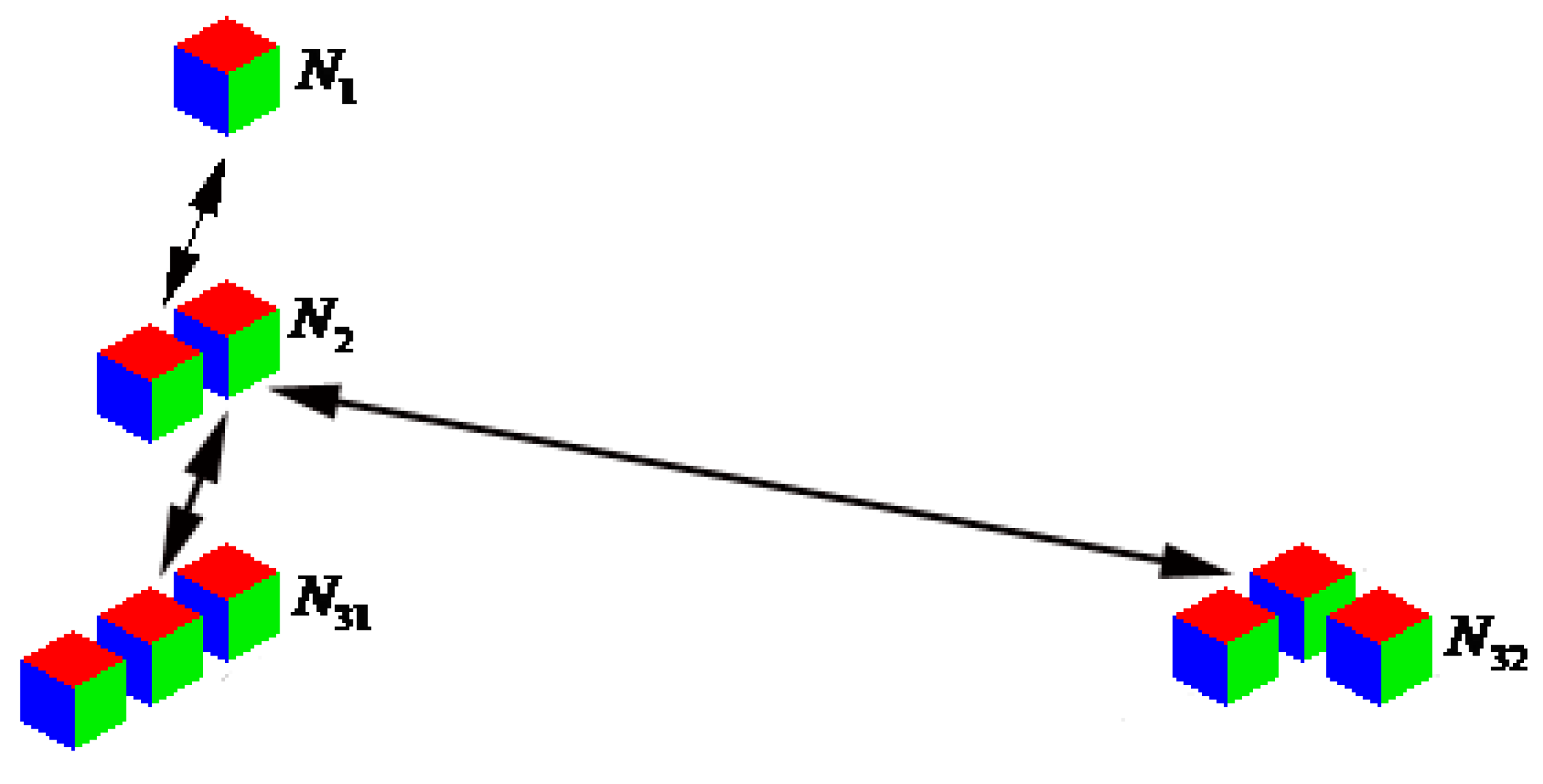
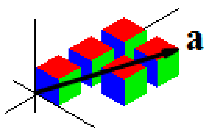
Consider another example, when not only the composition and mass of clusters, but also shape of clusters is taken into account. We confine ourselves to the case of aggregates consisting of no more than three original particles (molecules) and the shapes shown in Figure 1. The original particles are cubes here. We introduce the notation for the cluster concentrations, as shown in Figure 1: is a concentration of individual molecules, the aggregates of two molecules, and and are clusters of two shapes of the three molecules, and arrows indicate three possible reversible reactions.
Then, the evolution equations for these quantities read as:
Instead of the first equation of (5), we can take the conservation law of the number of all molecules in the system:
In (5), , , and are the constants (cross-sections, frequency functions) of the coalescence, and , , and are frequencies of fragmentation. Hereinafter, we write the rate constants of the processes as coefficients in equations as in Equation (3). The meaning of the indices in the coefficients in Equation (5) are clarified in the next section, where we define the notion of a shape consisting from cubes and write out a more general model via Equations (8)–(10).
Note that the systems in Equations (1) and (2) represent the physicochemical kinetics equations with an infinite number of reactions. The constants and in (1) and (2) are the rate coefficients of the processes if , and, if , then each of them gives a doubled reaction constant (in terms of Equation (3)). It is these constants (and not the coefficients of rates of the processes) that were introduced for the convenience of the writing of Equation (1).
In [6,7,11], a classification of the equations of physicochemical kinetics (3) is given according to the entropy principle: . Here C denotes the class of all systems of Equation (3) with a finite number of reactions. E is the class of systems for which the condition of semidetailed balance, or complex balance condition, or dynamical equilibrium is satisfied. This, as shown in [6,7,11,28], guarantees an increase of entropy. Boltzmann introduced the semidetailed balance condition for collisions in 1887 [28] and proved that it guarantees the positivity of the entropy production. The microscopic background for the semidetailed balance was found by Ernst Stueckelberg [29] in the Markov microkinetics of the intermediate compounds present in small amounts and whose concentrations are in quasiequilibrium with the main components. Under these microscopic assumptions, the semidetailed balance condition is just the balance equation for the Markov microkinetics according to the Michaelis–Menten–Stueckelberg theorem formulated by Gorban [30]. For chemical kinetics, this condition (known as the complex balance condition) was introduced by Horn and Jackson in 1972 [11]. is the class of systems of Equation (3) with detailed balance, and S is the class of systems with symmetric reaction constants (i.e., systems for which ). The concepts of detailed and semidetailed balance are explained below.
3. Results
3.1. The Simplest Models for the Evolution of Clusters Differing in Shape
We call the original particles constituting the cluster as adjacent if they have a common face. We assume that a cube attaches to an aggregate or to another original particle only in such a way that it becomes adjacent at least to one other original particle.
In the first simplest model we restrict ourselves to the investigation of modeling the evolution of clusters, differing in shape, for the Becker–Döring case, i.e., when only the original particles coalesce with and fragmentize from the cluster.
Each aggregate is characterized by the number n of constituting original particles. Moreover, for each cluster, we determine the minimum rectangular parallelepiped in which this cluster is placed so that the faces of the cubes, its components, are parallel to the corresponding faces of this parallelepiped. Such rectangular parallelepipeds are characterized by length, width, and height, i.e., the numbers , , , defining the vector , and we consider permutations of triplets of numbers as indistinguishable vectors. It is obvious that:
It makes sense to consider not only the 3-dimensional aggregates of the original particles, but also 2-dimensional ones, since the growth of clusters on the surface and the growth of films are of interest. Then, instead of cubes, we have squares that are connected to each other so that their edges coincide, and the analogue of condition (6) has the form:
In the 1-dimensional case, however, we obtain that , which returns us to the system of Equations (6) and (7). Therefore, we consider , where . Figure 2 shows an example of a vector . Note that in the 1-dimensional case (d = 1), we get the chains consisting of the original particles, and the breaking of one bond between two neighboring original particles in the chain leads to its breaking. This means the processes of agglomeration and fragmentation of chains become essential along with the processes of coalescence and fragmentation of individual original particles to the chain. Therefore, the 1-dimensional case of the evolution of clusters of different mass and shape under the Becker–Döring constraint makes sense to consider only when the growth of chains occurs on the surfaces, and then the system of equations describing the evolution has the form of (2).
For each , we define a finite set as the set of all vectors satisfying the condition (6) when ((7) when ). Thus, a shape is described by a pair , where , . The set of all such pairs we denote by .
Consider the evolution of the concentrations (or numbers) of the clusters having the shape : , . Without loss of generality, we assume here that .
We need to write a system of equations of the type of the physicochemical kinetics with all interactions of the form:
where , , is the zero vector, and () is a vector with one in -th place and zeros in the others. Here the vectors are such that and , and in any other cases, the coefficients of the direct and reverse reactions are assumed to be zero. If , then does not vary, but is increased by one in all four cases: .
For brevity, we introduce the notation for the number of individual original particles: .
The system of equations is:
Thus, here, is the cross-section (frequency function, reaction rate coefficient) of such coalescence of the original particle with the shape , at which increases by the value , so the shape is obtained; is the frequency of fragmentation of the shape into the original particle and the shape .
If for each and every , we do not distinguish the shapes and , then Equations (9) and (10) become the Becker–Döring case, Equation (2). However, our task is to distinguish the aggregates consisting of the original particles not only in mass, but also in shape.
In the second simplest model, we assume that, on the contrary, only rectangular parallelepipeds can coalesce with their identical faces, so that the result is a rectangular parallelepiped again. Thus, clusters without voids are obtained, i.e., Equations (1) and (2) become equalities. In the 3-dimensional case, we have:
For each , we define a finite set as the set of all triples of natural numbers satisfying the condition (11). Thus, due to the condition (11) in this model, a shape is described by a triple of numbers . The concentration (or the number) of aggregates having the shape in time moment is denoted by .
Define the function:
We obtain the following evolution equation for the concentration of the original particles or shape :
For the evolution of the concentration of the shape , we have:
Writing down a similar equation for the evolution of the concentration of an arbitrary shape , we obtain:
The last term here denotes the similar terms for and , which is written for . To avoid a repetition, such terms should be written out only for different numbers from a triplet . In Equations (12)–(14), the coefficients represent the reaction (process) constants.
The second simplest model (14) is a vectorial version of the classical discrete Smoluchowski coagulation–fragmentation equations [17], where some compatibility condition of the vectors is demanded. The compatibility is that the only vectors that can merge are those which differ in one component.
If there is an upper limit for : (), then we have the finite–dimensional system consisting from equations, which we call the M-th approximation of Equations (9) and (10):
Then, the shape is described by a pair , where , . We denote the set of all such pairs by .
Instead of the first equation of (15), we can write the conservation law of all original particles in the system:
For the second model, the -th approximation of (14) reads:
Then, instead of the equation for the evolution of N(1,1,1,t) in (16), we can write the conservation law of all the original particles in the system:
Thus, we obtain the systems of Equations (9), (10) and (14), as well as their M-th approximations (15) and (16). Now let us address the H-theorem point.
We consider the H-theorem for a finite system of equations. This faces the same difficulties with convergence of series for the infinite systems as discussed in [18,19,20,21]. It is important to point out that the detailed study of the H-theorem in this case is a problem for a separate paper. Nevertheless, our results involve the detailed balance and so are valid regardless of the finiteness of the systems in question.
3.2. The Conditions of Detailed and Semidetailed Balance
The condition of the detailed balance for the general system of equations of physicochemical kinetics (3) is actually the condition for the coefficients: let there exist at least one positive solution of the following system of equations:
This assumes that the rate of the direct reaction is equal to the rate of the reverse reaction for all the reactions. The number of equations in the detailed balance condition is equal to the number of reactions which is half of the number of pairs in set , while the number of unknowns equals .
The condition of detailed balance in the case of Equations (9) and (10) takes the following form: let there be at least one solution () of the system:
where and for all .
The condition of semidetailed balance [6,7,11,24,28,29] is a condition when there is at least one positive solution of the following system of equations:
Here, is defined so that with some . The sum runs only over those multi-indices for which either or . The sum of the rates of all reactions with initial state is equal to the sum of all rates of reactions with final state . The number of equations in the condition of semidetailed balance is half of the number of different vectors in pairs .
The condition of semidetailed balance in the case of Equations (9) and (10) leads to the two types of relations:
and:
Note that the relations of the form of (18) determine the recursion: expresses through and if .
The condition of detailed balance as well as the condition of semidetailed balance imposes restrictions on the cross-sections. If we consider these conditions for the M-th approximation of the Equations (9) and (10), i.e., for (15), then, this case contains some restrictions of the original case remaining unchanged. Therefore, it is advisable to consider examples of systems of the form (15).
Consider an example when : each of shapes with and is unique, there are two shapes with , and there are three shapes with in the 2-dimensional case and four shapes in the 3-dimensional case.
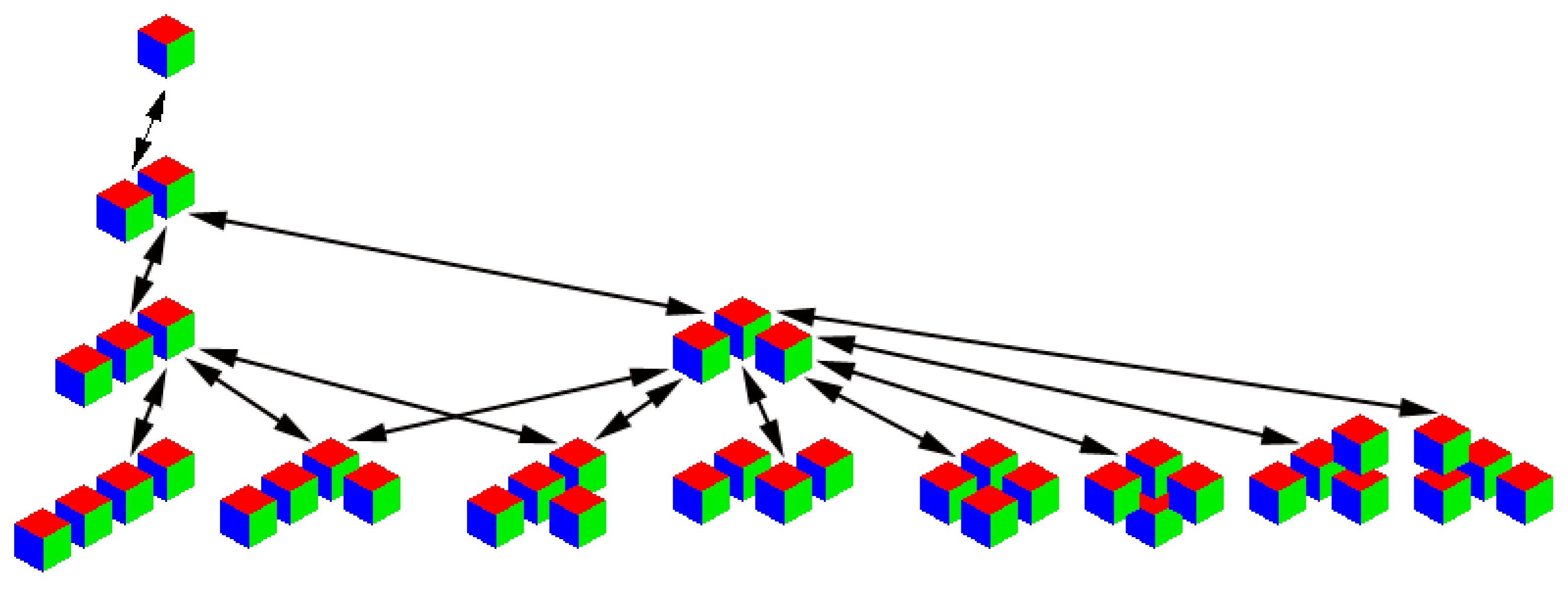
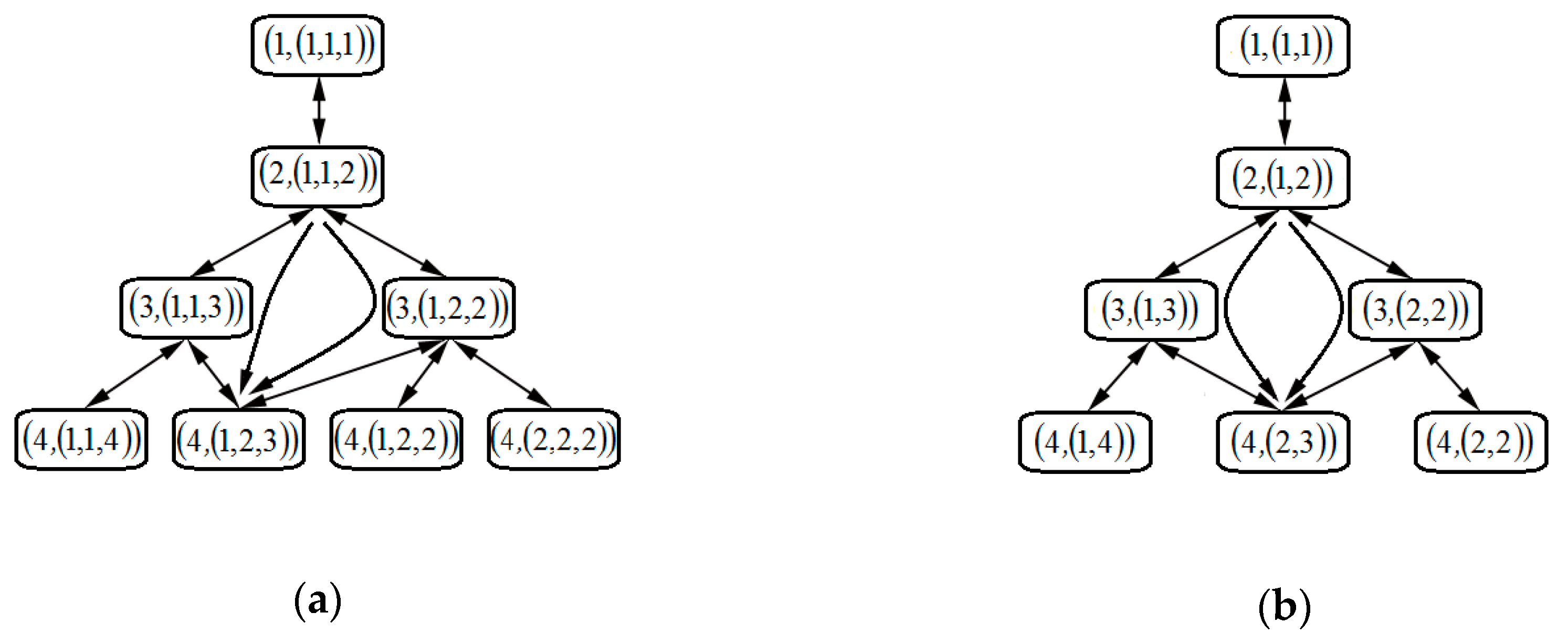
Natural shapes from cubes with and reactions are shown in Figure 3, and a similar scheme (graph) for our model for the 3- and 2-dimensional cases is shown in Figure 4a,b, respectively. The naturalness is defined as follows: the clusters have the same shape if they are transferred into each other by transformation of motion that does not change the orientation in space. The fact that the original particles have a reaction with a specific shape is not depicted here.
Due to the condition of detailed balance in this example (), we have the following restriction on cross-sections for (Figure 4a):
which comes from the fact that starting from the node one gets the node in two different ways. Restrictions on the cross-sections come in play as soon as the resulting graph is not a tree, i.e., contains various reaction paths.
In the case of shapes, the graph in Figure 3 is different, and the condition of detailed balance leads to the two relations (similar to (20)).
The case of a stationary solution, when there are neither detailed nor semidetailed balances, is shown in Figure 5, which corresponds not only to Figure 3 but also to Figure 4.
Let us consider an example for this situation, i.e., a system of equations where only aggregates shown in Figure 5 are considered. Simply let us record the equations by entering notations for cluster concentrations, as shown in Figure 5 (and as it was given in the example in the introduction): is the number of aggregates of two original particles, and are the concentrations of aggregates of two types of three original particles, and of four. Then, we obtain a counterpart of (15):
replacing the evolution equation of concentration N1 with the conservation law of the number of all original particles in the system:
Obviously, the condition that the vector is a stationary solution of (21) and (22) is equivalent to the fact that, for some number , the vector satisfies the system
and:
In Figure 5, the directions of the arrows indicate the direction of the process: coalescence prevails with the original particle or fragmentation. If and only if all four reactions in Figure 5 have the same magnitude of “dominance”, then one obtains the stationary solution that satisfies (23). Indeed, the number of arrows “up” is equal to the number of arrows “down” and, therefore, the number of original particles is preserved. For the aggregates from the original particles, this is also immediately apparent from Figure 5, where exactly one arrow comes and goes to each vertex of the graph. The directions of the arrows in Figure 5 correspond to in (23). The detailed balance (the semidetailed balance) is the case when the value of the “predominance” of all reactions is zero: .
If the of value is fixed, then (23) becomes a linear system. The condition of detailed balance of Equation (20) is the condition that the determinant of this system is zero.
In its turn, if the determinant of this system is zero, one obtains positive stationary solutions that satisfy the detailed balance condition, which is the solution of Equations (23) and (24) with . By virtue of the H-theorem, we obtain that such a stationary solution is unique and stable, if the value of the constant in (22) is fixed according to the initial data.
If the determinant is not zero, then there are no stationary solutions satisfying the condition of the detailed balance (except a trivial one when the vector is zero). However, in this case, for each positive value of in (22), we can find the stationary solution (21). As soon as the system of (23) is solved, as a linear system for fixed , the value of the constant is uniquely determined by the relationship (24) through the value , and so the value is calculated according to (22).
For Equation (14), the condition of semidetailed balance coincides with the condition of the detailed balance and has the form:
In general, for equations of the type of coagulation–fragmentation equations, it is typical that the condition of semidetailed balance coincides with the condition of detailed balance.
In the simplest models in Section 3.1, it is not yet clear what to take as a section, and it can be considered that the conditions of detailed or semidetailed balances are valid. Thus, we first need to consider the natural shapes of the original particles such as in Figure 3 and sections for them resulting from the physical models. Although we do not know how many shapes and how many ways there are of obtaining each of them from others, it is possible to prove that the condition of detailed balance for a specific physical model of the sections is fulfilled. First, we consider an anisotropic original particle; for these, the validity of condition of detailed balance is proven. Then, we do a transition to the isotropic case. We prove that the condition of detailed balance is maintained. This gives a method of obtaining kinetic equations describing the evolution of clusters of different masses and shapes.
After that, we prove the H-theorem under the condition of semidetailed balance (18) and (19). Then, the H-theorem is obtained under the condition of detailed balance, since Equations (18) and (19) are a consequence of the condition of Equation (17). For the second model, we consider the H-theorem under the condition of detailed balance (25), which coincides with the condition of semidetailed balance.
3.3. The Condition of Detailed Balance, the Arrhenius Law and the Model of the Evolution of Clusters Differing in Shape
The condition of detailed balance for the general system of physicochemical kinetics Equation (3) is:
If we (formally) put:
Equation (26) can be rewritten in the following form:
where , is the energy of the state participating in reactions of the form (4), is the Boltzmann constant, is the temperature of the medium, and is the canonical partition function. Equation (27) is the Boltzmann equation for the probability of a given state. We connect the Boltzmann equation with the principle of the detailed balance and obtain that as soon as the principle of detailed equilibrium is satisfied, then the reaction constants can be written in the form:
where are symmetric coefficients.
In 1889, in “On the reaction rate of the inversion of cane sugar under the influence of acids”, Svante Arrhenius posited the relationship of the dependence of the rate constant of the chemical reaction on temperature [31], which today is called the Arrhenius equation or Arrhenius law (actually originally proposed by Vant Goff) [32,33]. The Arrhenius law for the system of equations of chemical kinetics (3) has the form:
Here, is the activation energy of the reaction in Equation (4). The activation energy is the energy of molecules in a collision, the level of which is sufficient to carry out the chemical reaction of Equation (4). Here, as is shown below, the coefficients are asymmetric: , unlike in Equation (29).
From (30), we obtain that, for the equilibrium, the following relations for the reaction rate constants hold true:
Note that (31) is a more general condition than (30) in cases, where the rate constants of all reactions are given.
Let for all :
i.e., the activation energy is an additive quantity. Then, relationship (31) takes the form:
Comparing Equations (28) and. (33), we obtain that .
Generally, one can explain the relationship (32) and follow more closely the concept of the activation energy as soon as the concept of the so-called energy diagrams of reactions is used.
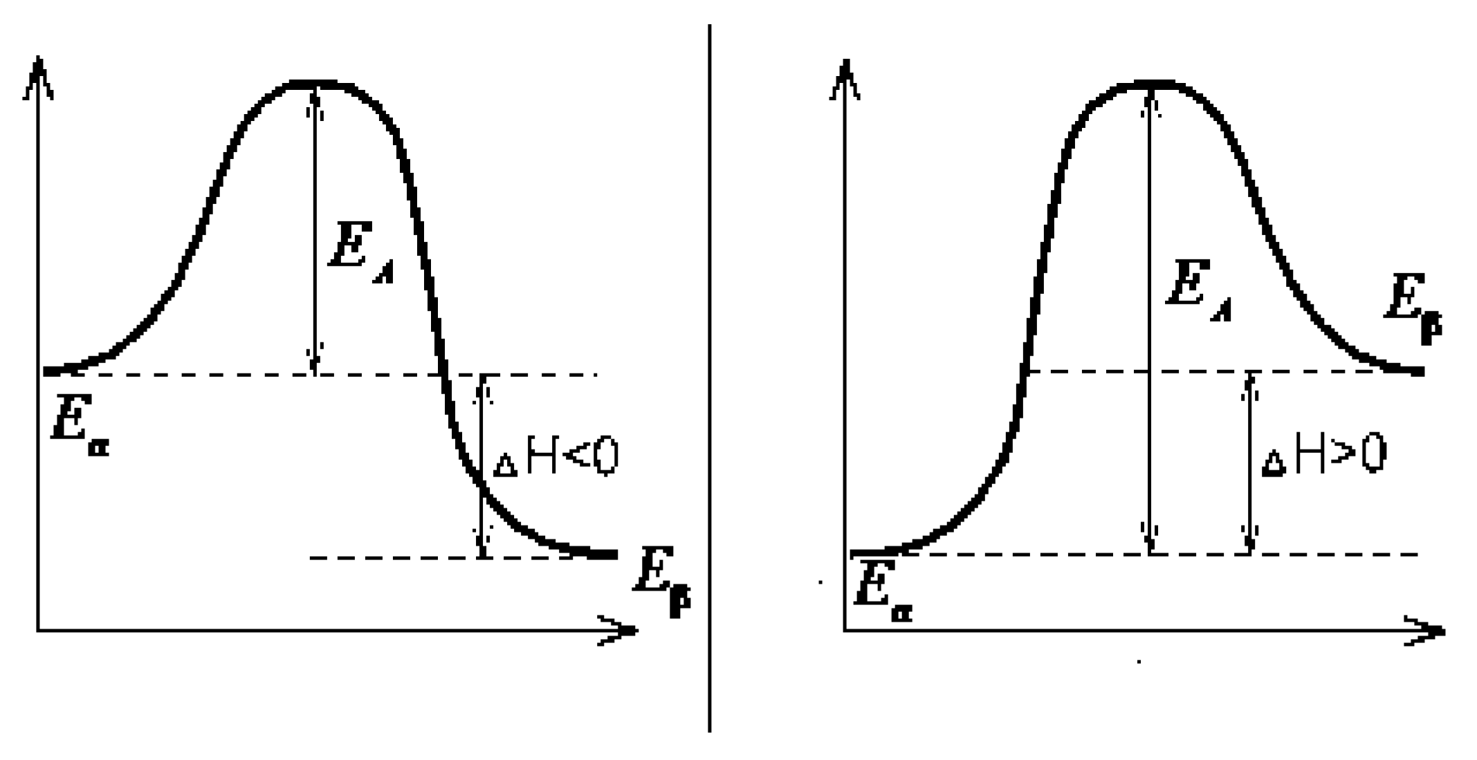
If the activation energy of reaction in Equation (4) (see Figure 6), then the activation energy of the inverse reaction is , where is the energy of the initial complex and is the energy of the final product . Therefore, relationship (32) is satisfied: . This is the variation in enthalpy as a result of the reaction (see Figure 6).
Theorem1.
Let relationship (33) hold for all. Let, then, that for the system:
there is a positive stationary solutionthat satisfies the condition of detailed balance:, .
Then:
(a) For Equation (3),
there is a stationary solution: , satisfying the detailed balance condition (26);
(b) The H-function for Equation (3) differs from the H-function for Equation (34):
by the amount, i.e., has the form:
The H-function (35) does not increase by the solution of Equation (3):. All stationary solutions of Equation (3) satisfy equalities of Equation (26);
(c) Equation (3) hasconservation laws of the form (), whereis the dimension of the linear envelope of the vectors(Boltzmann–Orlov–Moser–Bruno vectors [16,26,27]), and the vectorsare orthogonal to all : . The stationary solution of Equation (3) is unique, all the constantsare fixed, and it is given by:
whereare determined by thevalues;
(d) Such a stationary solution exists ifis determined by the initial condition—a vector with non-negative components: . A solutionwith this initial condition exists for all, is unique, and tends to the stationary solution (36).
Proof.
The H-theorem for the chemical kinetics equations with a finite number of reactions under the condition of detailed balance was considered in [6,7]. By virtue of it, the Theorem 1 is obvious. □
From (31) and the detailed balance conditions, , we obtain the basic equation of thermodynamics:
where . is entropy change as a result of the reaction.
Now we consider the frequency functions for our case, analyze them in terms of relationships (30) and (32), and check the fulfillment of the condition of detailed balance for them.
Frequency functions in general form are unknown, but according to numerous observations, in the case of gases (vapors) they look like (40) and (41) below, see [23]. In this section, we show that the condition of detailed balance is satisfied for such sections.
In addition, we explain how the frequency functions are obtained from theoretical considerations. There are two main theories of molecular kinetics, namely, the theory of active collisions and the theory of an activated complex [32,33,34,35,36,37].
According to the first of these, so-called active collisions lead to chemical reactions—collisions of those particles for which the value of the energy of relative motion along the line of the centers of the colliding particles exceeds a certain value, the activation energy.
The basic equations of the theory of active collisions were obtained by Max Trautz in 1916 [34] and William Lewis in 1918 [35]. A comparison of the total number of collisions and the number of active collisions shows that a large number of inactive collisions occur between the acts of reactions that require activation energy. Therefore, it is assumed that the particle velocity distribution functions are equilibrium or Maxwellian, and chemical transformations do not violate this statistical equilibrium.
Then, within the framework of the theory of active collisions, the equations of chemical kinetics (for the case of pairing interactions) can be obtained from the Boltzmann equation [10] as in the transition to hydrodynamics in the case of a zero order approximation in the Chapman–Enskog method (transition to Euler equations) [6]. Indeed, we present the collision integral as a sum of all elastic (inactive) collisions and the integral of inelastic (active) collisions. Then, substituting the Maxwell distribution into such equations (written for each i-th type of particles), integrals of the first type vanish, and the second (after integrating both parts of the equation over the space of velocities) gives the right-hand side of the i-th equation of the system of (3). As a result, in spatially homogeneous cases, one obtains equations of (3).
For simplicity, we restrict ourselves to the study of modeling the evolution of clusters, which differ in shape, for the Becker–Döring case, i.e., when only the original particles coalesce with and fragmentize from the aggregate.
Thus, in our problem, the cross-section for coalescence is a shape with the original particle that can be modeled using the theory of active collisions (see below). When considering the fragmentation, one has to apply the theory of an activated complex: the original particles fragmentize from the aggregates not because they are knocked out by environmental particles by direct collision, but because the entire aggregate is in a disturbed state due to collisions with particles of the medium and emits those initial particles off their surface, the energy of which is greater than the activation energy of the process, the binding energy with the rest of the aggregate particles.
The surface of an aggregate consisting of original particles defines a set of “seats” for coalescence with a single original particle, which results in the aggregate consisting of the original particles.
Let us introduce the notation for the combinatorial numbers, which arise in the consideration of shapes and transitions between them as a result of coalescence with or departure of a single original particle. Let a shape be obtained from a shape by the addition of one original particle. Let denote the number of ways to obtain shape from shape (the number of “seats” of shape , which after coalescence with a single original particle gives shape ). Here, the superscript “(1)” denotes the original particle. We denote a number of ways of obtaining from in the result of the fragmentation of a single original particle from through .
For example, from Figure 1, we can see that for and for , where“(2)” denotes dimmer, because a cube has six faces, i.e., six “seats”, and a square has four sides, i.e., four “seats” in the 2-dimensional case.
Generally speaking, . Indeed, as can be seen from Figure 1, for the reaction of formation of one (left) of the shapes of aggregates, consisting of three original particles, as a result of coalescence an original particle with an aggregate of the two original particles, both these numbers are equal to two, and for the reaction of formation of the other (right) shape , and for ( for ).
Let us consider the case of anisotropic particles. First, let us define what the anisotropy means using an example where the original particles are cubes, and then get a common definition of the anisotropic particles. Anisotropic shapes can be represented, for example, by means of the following mental model. We can represent anisotropic shapes as particles consisting not of cubes but of rectangular parallelepipeds, whose length, width, and height are different and the opposite faces are numbered “1” and “2”. The point is that all faces of original particles are different. These particles coalesce with a single original particle only so that faces of integrating original particles are the same by size and have different numbers: a face numbered “1” can merge with a face with the same size numbered “2” (or “2” vs. “1”). In this case, one obtains: .
For shapes, consisting of such original particles, and are equal to 1. Here, we notice a feature where, for straight chains of molecules, they are equal to 2, while the relationship is always satisfied. This gives a generalization of the definition of anisotropy from the case of cubes to the arbitrary shapes of the original particles. The definition is simple: .
For the coalescence of an aggregate, consisting of original particles, with a single original particle that results into the aggregate consisting of the original particles, each “seat” corresponds to an effective section of interaction. As a result, an original particle occupies the “seat” if its energy is sufficient for such a reaction. We use the assumption that all such sections can be considered identical, i.e., independent of the “seat”. We denote them through .
Let us calculate the number of collisions of the “seat” with the flow of original particles falling onto the aggregates at a relative speed and consider the velocity distributions to be Maxwell distribution. Then, the corresponding average number of collisions of the original particles of mass with aggregate of original particles is equal to , where is the average of the absolute value of the relative velocity of original particles and aggregates, is their reduced mass, and here is the concentration, but not the number of original particles.
Therefore, if all the collisions result in the attachment of the original particle to the aggregate, then the rate constant for the reaction of coalescence of a shape with an original particle, which results in a shape , is equal to
since the number of “seats” of shape , resulting in shape , as soon as the original particle is attached, is equal to .
According to the theory of active collisions, it is believed that only those original particles for which the kinetic energy of relative motion along the line of centers of the colliding particles is greater than the activation energy E1 enter the reaction. Therefore, to calculate the rate constant coalescence of shape X with the original particle, we obtain the value (37) multiplied by some function of . This function has the form:
where g is a certain function, g(0) = 1, and significant dependence upon is included in the second factor. Therefore, by virtue of Equations (37) and (38), we have:
The activation energy may depend on the mass of an aggregate, , but we suppose that there is no dependence on the shape. Note that depends on even if , since depends on the .
Therefore, calculating the coalescence cross-sections , we restrict ourselves to the case of gases and the Maxwell–Smoluchowski model, since there are still no well-founded models for liquids. According to Maxwell, the collision cross-sections (for gases) are proportional to the surface area, and therefore a multiplicative coefficient appears in Equations (37) and (39). Smoluchowski accepted that if only the fraction of molecules falling on a particle leads to their coalescence with the particle, then the rate of coalescence must also change the factor (38) [17]. From the point of view of the theory of active collisions, this factor returns us to the Arrhenius law in the relationship (39).
If we neglect the difference of the function from one (due to the fact that ), then only in Equation (39) determines the fraction of active collisions. We assume that only the exponential factors in (30) determine the portion of active collisions. Then, Equation (34) describes the case with each collision leading to a reaction.
The frequency of fragmentation of shape to the original particle and shape is equal to [23]:
where is the Planck’s constant, is the correction factor, indices number original particles, constituting shape , the fragmentation of each of which gives shape , and is the activation energy of separation of the -th original particles of such type. In the second equality in (40), we have taken into account that does not depend on : is the activation energy for the fragmentation of the original particle from shape , a result of which is shape . The theoretical substantiation of the expression of (40), as already noted, is given by the theory of the activated complex [32,33,36,37].
At the same time, the activation energy of fragmentation is advisable to search in the form of the sum of activation energies required to break the connection with each of the nearest neighbors (close-range interaction): , , and overcome the attraction to all the original particles constituting the cluster (long-range interaction), the energy of which is :
is sought in the form:
which allows an extrapolation to the Gibbs–Thomson equation [23]. This equation forms the basis of the classical theory of nucleation. Here, is the activation energy of overcoming the attraction to an infinitely large particle, and and are the coefficients describing the decrease in attraction due to the decrease of . As is shown below, the form of the long-range interaction is completely irrelevant.
So far, we considered a pair of arbitrary shapes, one obtained from another by coalescence or fragmentation of one original particle, and termed them and . Now, consider a single arbitrary shape, which, in particular, may coincide with or , and term it .
Consider in a shape for each original particle, its component, the sum of the activation energies necessary for breaking the connection with each of the nearest neighbors. Let us sum them over all the original particles of shape and divide the obtained value by two, so that there are no duplicates in the summation of energies. Then, the energy calculated in this way can be called the energy of the close-range interaction of shape , . Thus, for every shape , the energy of close-range interaction is determined.
Then, the first term in (41) is the difference between the energies of the close-range interaction of shapes and . The second term, , can be interpreted as the increment of energy of the long-range interaction in the transition from the shape, consisting of original particles, to the shape consisting of original particles.
One may not separate the energies of the close-range and long-range interactions. This corresponds to the fact that in Equation (41), the neighbors closest to the considered original particle of the cluster, consisting of original particles, are all of its other original particles, i.e., , and .
Thus, generally speaking, for each shape we attribute the energy of the close-range interaction , for which the following condition of the additivity is fulfilled:
Then, by virtue of Equations (40) and (42), we obtain that:
where .
In virtue of Equations (39) and (43) for equilibrium constants , the following form of relations (33) is valid:
If , then it is impossible to talk about the fulfillment of additivity Equation (32), and Theorem 1 cannot be directly applied. However, dependence can be made in the pre-exponential factor . As such, Theorem 1 is applicable, and the only thing that remains to be checked is the implementation of the detailed balance for the equilibrium constants , corresponding to the equilibrium constants .
The condition of detailed balance for some model of shapes is satisfied if all possible relations are similar to Equation (20) for this model. We must prove that these relations are valid for any two (different) paths along the edges of the graph from the shapes (as in Figure 3) such that their beginnings and their ends coincide: and . The number of fractions on the right and left sides of such relations is the same and equal to the difference in the number of original particles in and , i.e., . For anisotropic original particles () in the right and left parts of such relations, there are identical expressions, and therefore the condition of detailed balance is satisfied, even if in (43) depends on . For isotropic particles, it is to show that the following relations are valid:
For each isotropic shape , we consider the set of all different anisotropic forms that give shape . We denote the cardinality of this set as .
Consider two isotropic shapes: and , where is obtained from by the attachment of original particles (with ways, and is obtained from by fragmentation of an original particle by ways). Consider a graph consisting of a set of vertices and all edges (reactions) connecting vertices from a set with vertices from . The number of such edges, emanating from the vertices belonging to , is , and this number is for the edges which emanate from the vertices belonging to . Therefore:
Note that it is namely due to the fact of the validity of the relations of the form of (45) that the system of kinetic equations for isotropic shapes can be derived from the evolution equations for anisotropic shapes. For this, for each isotropic shape all the anisotropic shapes from the set are identified, and the sum of all their concentrations is the concentration of shape . Then, by virtue of (45) equations for isotropic forms with correct cross-sections (containing the correct values of the coefficients , ) are obtained from the evolution equations for anisotropic forms.
In virtue of the relationship (45), Equation (44) is equivalent to:
which actually seems to be obvious.
This means that the condition of detailed balance is valid for the kinetic equations of evolution of both anisotropic and isotropic shapes from the original particles.
Therefore, the following is proven.
Theorem2.
Let the Becker–Döring case be considered, and the frequency functions are defined by Equations (39) and (43), being customary for gases (i.e., calculated according to the theory of active collisions and the theory of an activated complex), namely:
Let the assumption of independence of values of the cross-sections from the “seats” formulated above be valid. Then the conditions of detailed balance and the H-theorem are fulfilled.
3.4. The Linear Conservation Laws and the Convergence to the Equilibrium
The consequence of the H-theorem for the equations is the convergence of solutions to the Boltzmann extremal [1,3], i.e., to the argument of the conditional minimum of the H-function, provided that the constants of linear conservation laws are fixed. The role of linear laws remains somewhat mysterious, but they turn out to be regulators in various situations [1,3,6].
Lemma1.
The number (concentration) of all original particles is the only linear conservation law for the system in Equation (15):
and for Equation (16):
if the condition of detailed or semidetailed balance is valid.
Proof.
We first consider the first of our models—the system in Equation (15). Reactions (8) can be written in the form of (18):
The linear functional for Equation (15) has the form:
It is preserved along the solutions of (15) if vector is orthogonal to all the Boltzmann–Orlov–Moser–Bruno vectors (see Section 2 and Theorem 1c) [6,7,16,26,27]. Here, the condition of orthogonality gives the relations , where and . All such relations lead to an arithmetic progression on , and for any shape one gets: , i.e., the conservation law of the number of all original particles, , is the unique linear conservation law (up to a multiplicative constant). □
Similarly, for Equation (16), for the conditions of orthogonality of vector to the Boltzmann–Orlov–Moser–Bruno vectors, one obtains the following relations for any shape , :
where . From these by induction we get that , i.e., the only linear conservation law is the conservation law for the number of all original particles.
It is clear that for more complex models than those represented by Equations (15) and (16), the uniqueness of the conservation law of the number of all original particles can be proven the same way.
3.5. The Boltzmann Principle for the Simplest Model of the Evolution of Clusters of Different Masses and Shapes
Consider the system of equations in (15).
Let us show, for example, that the H-function:
decreases by the nonstationary solutions of Equation (15) under the condition of detailed balance (3):
The H-theorem for physicochemical kinetics equations with a finite number of reactions, under the condition of semidetailed balance was considered in [6,7,11]. Taking into account Lemma 1, we obtain the following formulation for the first of our simplest models.
Theorem3.
Let the coefficients for Equation (15) be such that there exists at least one positive solutionof the system of Equations (18) and (19).
Then:
(a) H-function (49) decreases by the solutions of (15):. All stationary solutions of Equation (15) satisfy the equalities of Equations (18) and (19);
(b) Equation (15) has a unique linear integral (an invariant of the form), and it is the conservation law of the number of all original particles:. The stationary solution of the system of Equation (15) is unique if we fix a constantand is given by the equation for the Boltzmann extremals (the argument of the minimum of H-function, provided that the constants of linear conservation laws are fixed):
whereis uniquely determined by the value of;
(c) Such a stationary solution exists if the constant of the conservation law of the number of all initial particles is determined by the initial condition. A solutionwith this initial condition exists for all, is unique, and tends to a stationary solution (50).
For the second of our simplest models, i.e,. for Equation (16), by Lemma 1, Theorem 3 is valid without changing, provided that there exists at least one positive solution of the system of Equation (25).
Thus, we obtain what the arbitrary solution of Equations (15) and (16) tends toward as soon as time tends to infinity. It is important to stress that this is deduced directly from the Boltzmann variational principle without solving the systems.
4. Conclusions
The main results are as follows: (1) we proposed a new model (or even a group of models) describing the shape of crystals; (2) we clarified the conditions for the applicability of the H-theorem to this group of models; (3) it was found that the Arrhenius condition implies a detailed balance for the new proposed simple models and for the general case of models.
Thus, we considered the issue of building correct (physically grounded) models of the evolution of cluster distribution functions for shapes based on the H-theorem (Boltzmann), which is being actively studied and is currently used in many mathematical problems of the natural sciences. We show that when building the models, it is necessary to monitor the fulfillment of the condition of detailed balance.
For simplicity, in Section 3, our study is limited to modeling the evolution of clusters that differ in shape for the Becker–Döring case, that is, when only the original particles coalesce with and are fragmented from the aggregate. It is interesting to generalize the result obtained (Theorem 2) to the case of the formation (and fragmentation) of aggregates consisting of agglomerates.
The simplest models of evolution of clusters, differing by shapes, are proposed in Section 3.1. The significance of these models is that the form of equations is the same as in the case of more detailed models.
It is of interest to generalize the results obtained to nonlinear systems with discrete time, in particular, even to construct discrete models of the Boltzmann equation with discrete time and to transfer the condition of semidetailed balance to discrete time. Consideration of the H-theorem for nonlinear systems with discrete time, in particular, even for the system of Becker–Döring equations, becomes an extremely important and urgent task, since computer modeling plays a key role in solving the fundamental problem of creating new materials [22,23]. In the linear case, when passing from continuous to discrete time, we have a transition from a Markov process to a Markov chain, and the H-theorem in this case is valid, as investigated earlier (see [8] and references therein). In the nonlinear case, it is valid in rare cases for explicit time discretization [8], and for the implicit case as investigated in [9].
These questions, as well as the results of the current work, clarify the point of constructing correct (physically grounded) kinetic models for the evolution of clusters differing in mass and other parameters.
At the same time, both for experimenters and calculators who deal with problems of modeling the evolution of such structures (for example, the problem of their optimal synthesis [22,23,38]), is extremely important that the number of parameters (numbers or functions) remain minimal (we have , , and activation energy in (46)), since the addition of at least one parameter or correction factor significantly increases the computational complexity of the problem.
Author Contributions
I.M. gave the general statement of the problem. All sections except Section 3.3 were written collectively during the authors’ discussions. V.V. linked the Boltzmann equation with the principle of detailed balance in Section 3.3. The remaining results in Section 3.3 were obtained by S.A. and J.B.
Funding
This paper was supported by the Ministry of Education and Science of the Russian Federation on the program to improve the competitiveness of Peoples’ Friendship University of Russia (RUDN-University) “5–100” among the world’s leading research and educational centers in 2016–2020.
Conflicts of Interest
The authors declare no conflicts of interest. The founding sponsors had no role in the design of the study; in the collection, analyses, or interpretation of data; in the writing of the manuscript, and in the decision to publish the results.
References
Boltzmann, L. Weitere Studien über das Wärmegleichgewicht unter Gasmolekülen. In Kinetische Theorie II; Vieweg Verlag: Wiesbaden, Germany, 1970; pp. 115–125. [Google Scholar] [CrossRef]
Godunov, S.K.; Sultangazin, U.M. On discrete models of the kinetic Boltzmann equation. Russ. Math. Surv.1971, 26, 1–56. [Google Scholar] [CrossRef]
Vedenyapin, V.V. Time averages and Boltzmann extremals. Dokl. Math.2008, 78, 686–688. [Google Scholar] [CrossRef]
Adzhiev, S.Z.; Vedenyapin, V.V. Time averages and Boltzmann extremals for Markov chains, discrete Liouville equations, and the Kac circular model. Comput. Math. Math. Phys.2011, 51, 1942–1952. [Google Scholar] [CrossRef]
Vedenyapin, V.V.; Adzhiev, S.Z. Entropy in the sense of Boltzmann and Poincaré. Russ. Math. Surv.2014, 69, 995–1029. [Google Scholar] [CrossRef]
Sinitsyn, A.; Dulov, E.; Vedenyapin, V. Kinetic Boltzmann, Vlasov and Related Equations; Elsevier Science: Waltham, MA, USA, 2011. [Google Scholar] [CrossRef]
Batishcheva, Y.G.; Vedenyapin, V.V. The second law of thermodynamics for chemical kinetics. Mat. Model.2005, 17, 106–110. [Google Scholar]
Adzhiev, S.Z.; Melikhov, I.V.; Vedenyapin, V.V. The H-theorem for the physico-chemical kinetic equations with explicit time discretization. Phys. A Stat. Mech. Appl.2017, 481, 60–69. [Google Scholar] [CrossRef]
Adzhiev, S.Z.; Melikhov, I.V.; Vedenyapin, V.V. The H-theorem for the physico-chemical kinetic equations with discrete time and for their generalizations. Phys. A Stat. Mech. Appl.2017, 480, 39–50. [Google Scholar] [CrossRef]
Horn, F.; Jackson, R. General mass action kinetics. Arch. Ration. Mech. Anal.1972, 47, 87–116. [Google Scholar] [CrossRef]
Vol’pert, A.I.; Hudjaev, S.I. Analysis in Classes of Discontinuous Functions and Equations of Mathematical Physics; Springer Netherlands: Dordrecht, The Netherlands, 1985. [Google Scholar]
Gorban, A.N.; Kaganovich, B.M.; Filippov, S.P.; Keiko, A.V.; Shamansky, V.A.; Shirkalin, I.A. Thermodynamic Equilibria and Extrema: Analysis of Attainability Regions and Partial Equilibria in Physicochemical and Technical Systems; Springer-Verlag: New York, NY, USA, 2001. [Google Scholar]
Losev, S.A.; Potapkin, B.V.; Macheret, S.O.; Chernyi, G.G. (Eds.) Physical and Chemical Processes in Gas Dynamics: Physical and Chemical Kinetics and Thermodynamics of Gases and Plasmas, Volume 2; American Institute of Aeronautics and Astronautics: Washington, DC, USA, 2004. [Google Scholar]
Vedenyapin, V.V.; Mingalev, I.V.; Mingalev, O.V. On discrete models of the quantum Boltzmann equation. Russ. Acad. Sci. Sb. Math.1995, 80, 271–285. [Google Scholar] [CrossRef]
Vedenyapin, V.V.; Orlov, Y.N. Conservation laws for polynomial hamiltonians and for discrete models of the Boltzmann equation. Theor. Math. Phys.1999, 121, 1516–1523. [Google Scholar] [CrossRef]
Smoluchowski, M. Versuch einer mathematischen Theorie der Koagulationskinetik kolloider Losungen. Z. Phys. Chem.1917, 92, 129–168. [Google Scholar] [CrossRef]
Carr, J. Asymptotic behavior of solutions to the coagulation-fragmentation equations. I. The strong fragmentation case. Proc. R. Soc. Edinb. Sect. A Math.1992, 121, 231–244. [Google Scholar] [CrossRef]
Carr, J.; da Costa, F.P. Asymptotic behavior of solutions to the coagulation-fragmentation equations. I. Weak fragmentation. J. Stat. Phys.1994, 77, 89–123. [Google Scholar] [CrossRef]
Ball, J.M.; Carr, J.; Penrose, O. The Becker-Döring cluster equations: Basic properties and asymptotic behavior of solutions. Commun. Math. Phys.1986, 104, 657–692. [Google Scholar] [CrossRef]
Ball, J.M.; Carr, J. Asymptotic behavior of solutions to the Becker-Döring equations for arbitrary initial data. Proc. R. Soc. Edinb. Sect. A Math.1988, 108, 109–116. [Google Scholar] [CrossRef]
Melikhov, I.V. The evolutionary approach to creating nanostructures. Nanosyst. Phys. Chem. Math.2010, 1, 148–155. [Google Scholar]
Malyshev, V.A.; Pirogov, S.A. Reversibility and irreversibility in stochastic chemical kinetics. Russ. Math. Surv.2008, 63, 1–34. [Google Scholar] [CrossRef]
Gasnikov, A.V.; Gasnikova, E.V. On entropy-type functionals arising in stochastic chemical kinetics related to the concentration of the invariant measure and playing the role of Lyapunov functions in the dynamics of quasiaverages. Math. Notes2013, 94, 854–861. [Google Scholar] [CrossRef]
Moser, J.K. Lectures on Hamiltonian Systems; American Mathematical Society; New York University: New York, NY, USA, 1968. [Google Scholar]
Bruno, A.D. The Restricted 3-Body Problem: Plane Periodic Orbits; Walter de Gruyter: Berlin, Germany, 1994. [Google Scholar]
Boltzmann, L. Neuer Beweis Zweier Sätze Über Das Wärmegleichgewicht Unter Mehratomigen Gasmolekülen; K.K. Hof-und Staatsdruckerei: Vienna, Austria, 1887. [Google Scholar] [CrossRef]
Stueckelberg, E.C.G. Theoreme H et unitarite de S. Helv. Phys. Acta1952, 25, 577–580. [Google Scholar] [CrossRef]
Melikhov, I.V.; Rudin, V.N.; Kozlovskaya, E.D.; Adzhiev, S.Z.; Alekseeva, O.V. Morphological memory of polymers and their use in developing new materials technology. Theor. Found. Chem. Eng.2016, 50, 260–269. [Google Scholar] [CrossRef]
Arrhenius, S. Über die Reaktionsgeschwindigkeit bei der Inversion von Rohrzucker durch Säuren. Z. Phys. Chem.1889, 4U, 226–248. [Google Scholar] [CrossRef]
Stiller, W. Arrhenius Equation and Non-Equilibrium Kinetics: 100 Years Arrhenius Equation; B.G. Teubner Verlagsgesellschaft mbH: Stuttgart, Germany, 1989. [Google Scholar]
Laidler, K.J.; Klng, M.C. The Development of Transition-State Theory. J. Phys. Chem.1983, 87, 2657–2664. [Google Scholar] [CrossRef]
Trautz, M. Das Gesetz der Reaktionsgeschwindigkeit und der Gleichgewichte in Gasen. Bestätigung der Additivität von Cv-3/2R. Neue Bestimmung der Integrationskonstanten und der Moleküldurchmesser. Z. Anorgan. Allgem. Chem.1916, 96, 1–28. [Google Scholar] [CrossRef]
Lewis, W.C.McC. LXX.—Studies in catalysis. Part V. Quantitative expressions for the velocity, temperature-coefficient, and effect of the catalyst from the point of view of the radiation hypothesis. J. Chem. Soc. Trans.1916, 109, 796–815. [Google Scholar] [CrossRef]
Kubasov, A.A. Chemical Kinetics and Catalysis, Part 2: Theoretical Foundations of Chemical Kinetics; Lomonosov Moscow State University: Moscow, Russia, 2005. [Google Scholar]
Belousov, N.V. Chemical Kinetics: The Electronic Course for Universities; IPK SFU: Krasnoyarsk, Russia, 2009. [Google Scholar]
Gorban, A.N.; Shahzad, M. The Michaelis–Menten– Stueckelberg Theorem. Entropy2011, 13, 966–1019. [Google Scholar] [CrossRef]
Figure 1.
The aggregates, consisting of no more than three original particles (cubes), and their concentrations. is a concentration of individual molecules, are aggregates of two molecules, and and are clusters of two shapes of the three molecules. The arrows indicate three possible reversible reactions.
Figure 2.
The example of the vector , characterizing the shape of the particle consisting of original particles. Here, , .
Figure 2.
The example of the vector , characterizing the shape of the particle consisting of original particles. Here, , .
Figure 3.
The aggregates, consisting of no more than four original particles.
Figure 3.
The aggregates, consisting of no more than four original particles.
Figure 4.
The shapes of aggregates, consisting of no more than four original particles, for the first simplest d-dimensional model: (a) , (b) .
Figure 4.
The shapes of aggregates, consisting of no more than four original particles, for the first simplest d-dimensional model: (a) , (b) .
Figure 5.
The minimum set of aggregates, for which the condition of detailed and semidetailed balance can be not valid, and their concentrations. Directions of the arrows indicate which of the direction of the process prevails: coalescence with the original particle or fragmentation.
Figure 5.
The minimum set of aggregates, for which the condition of detailed and semidetailed balance can be not valid, and their concentrations. Directions of the arrows indicate which of the direction of the process prevails: coalescence with the original particle or fragmentation.
Figure 6.
The energy diagram of the reaction: is the activation energy of reaction, is the energy of the initial complex , is the energy of the final product , and is the variation in enthalpy as a result of the reaction.
Figure 6.
The energy diagram of the reaction: is the activation energy of reaction, is the energy of the initial complex , is the energy of the final product , and is the variation in enthalpy as a result of the reaction.
Adzhiev, S.; Batishcheva, J.; Melikhov, I.; Vedenyapin, V.
Kinetic Equations for Particle Clusters Differing in Shape and the H-theorem. Physics2019, 1, 229-252.
https://doi.org/10.3390/physics1020019
AMA Style
Adzhiev S, Batishcheva J, Melikhov I, Vedenyapin V.
Kinetic Equations for Particle Clusters Differing in Shape and the H-theorem. Physics. 2019; 1(2):229-252.
https://doi.org/10.3390/physics1020019
Chicago/Turabian Style
Adzhiev, Sergey, Janina Batishcheva, Igor Melikhov, and Victor Vedenyapin.
2019. "Kinetic Equations for Particle Clusters Differing in Shape and the H-theorem" Physics 1, no. 2: 229-252.
https://doi.org/10.3390/physics1020019
APA Style
Adzhiev, S., Batishcheva, J., Melikhov, I., & Vedenyapin, V.
(2019). Kinetic Equations for Particle Clusters Differing in Shape and the H-theorem. Physics, 1(2), 229-252.
https://doi.org/10.3390/physics1020019
Article Metrics
No
No
Article Access Statistics
For more information on the journal statistics, click here.
Multiple requests from the same IP address are counted as one view.
Adzhiev, S.; Batishcheva, J.; Melikhov, I.; Vedenyapin, V.
Kinetic Equations for Particle Clusters Differing in Shape and the H-theorem. Physics2019, 1, 229-252.
https://doi.org/10.3390/physics1020019
AMA Style
Adzhiev S, Batishcheva J, Melikhov I, Vedenyapin V.
Kinetic Equations for Particle Clusters Differing in Shape and the H-theorem. Physics. 2019; 1(2):229-252.
https://doi.org/10.3390/physics1020019
Chicago/Turabian Style
Adzhiev, Sergey, Janina Batishcheva, Igor Melikhov, and Victor Vedenyapin.
2019. "Kinetic Equations for Particle Clusters Differing in Shape and the H-theorem" Physics 1, no. 2: 229-252.
https://doi.org/10.3390/physics1020019
APA Style
Adzhiev, S., Batishcheva, J., Melikhov, I., & Vedenyapin, V.
(2019). Kinetic Equations for Particle Clusters Differing in Shape and the H-theorem. Physics, 1(2), 229-252.
https://doi.org/10.3390/physics1020019
