Article

Metamorphic Malware Detection via Graph-Augmented Neural Semantics and Adversarial Hardening: A Comprehensive Framework


by
Victor Manuel González-Gorrín
* and
Josep Prieto-Blázquez
Faculty of Computer Science, Multimedia and Communications, Universitat Oberta de Catalunya, Rambla del Poblenou, 154-156, 08018 Barcelona, Spain
*
Author to whom correspondence should be addressed.
J. Cybersecur. Priv. 2026, 6(5), 164; https://doi.org/10.3390/jcp6050164 (registering DOI)
Submission received: 27 July 2026 / Revised: 6 September 2026 / Accepted: 14 September 2026 / Published: 17 September 2026
(This article belongs to the Special Issue Cyber Security and Digital Forensics—3rd Edition)

Abstract

Background: Metamorphic malware is among the most persistent adversarial challenges in cybersecurity: it rewrites its own instruction stream on every propagation, preserving functional semantics while presenting a syntactically distinct binary that defeats signature-based and many learning-based detectors. Methods: We propose MetaGNN-Sec, a graph-augmented neural framework that detects metamorphic malware from program structure rather than surface bytes. The framework composes four components, each addressing a distinct facet of the problem: (i) control-flow graph (CFG) extraction with semantic opcode embeddings; (ii) a heterogeneous graph neural network (hGNN) operating over program-dependence graphs that capture mutation-stable control- and data-flow invariants; (iii) an adversarial training loop derived from the Wasserstein generative adversarial network (WGAN) that hardens the classifier against adaptive evasion mutations; and (iv) a quantum-kernel anomaly layer implemented in PennyLane for separation of heavily obfuscated outliers in a high-dimensional feature space. Results: Experiments are conducted on two public corpora—VirusShare 2024 and a SOREL-20M subset—comprising 200,175 binary samples in total (155,175 malware and 45,000 benign), in agreement with the corpus totals reported in Datasets Section of this paper. MetaGNN-Sec achieves a detection rate of 97.83%, a false-positive rate of 0.41%, and an F 1 score of 0.978 on held-out metamorphic families, exceeding the next-best baseline (MalConv+) by 4.6 percentage points on clean data and degrading by only 5.4 points under adaptive adversarial evasion (versus 17–31 points for the baselines). The quantum-kernel module contributes a further 1.2 pp reduction in false-negative rate, concentrated on the most heavily mutated families. Conclusions: The framework provides a heterogeneous PDG representation with a conditional score-shift bound under graph-edit-bounded mutations, a WGAN hardening loop that delivers measurable adversarial robustness, a quantum-kernel pre-filter with an explicit cost/benefit characterization, and a reproducible, near-real-time pipeline suitable for enterprise endpoint deployment.

1. Introduction

The malware landscape has undergone a profound structural shift over the past decade. Whereas first- and second-generation threats relied on static byte signatures that were straightforwardly matched by antivirus engines, contemporary adversaries routinely deploy metamorphic code—programs that autonomously rewrite their own instruction streams at each propagation cycle while preserving observable behavior [1,2,3,4,5]. Unlike polymorphic variants, which merely encrypt a fixed payload beneath a variable decryption stub, metamorphic engines perform semantics-preserving transformations including dead-code insertion, register reassignment, instruction substitution, subroutine permutation, and control-flow transposition [6,7]. These transformation classes are not abstract: they are realized by documented engines operating on the x86/x86-64 instruction-set architecture, and our usage follows the canonical taxonomy of You and Yim [4] and the control-flow-transposition analysis of Borello and Mé [6]. The result is a family of binaries that share a common functional ancestry yet may exhibit vanishingly small byte-level similarity [8].
Signature-based detection, by construction, fails against such threats [9]. Statistical and machine learning approaches fare better but remain vulnerable to adversarial perturbations that deliberately exploit the decision boundary of a trained classifier [10,11]. Concurrently, the rapid proliferation of large-scale binary repositories—VirusShare alone catalogs over 50 000 000 samples—demands detection pipelines capable of processing millions of binaries per day with minimal human supervision.
Recent advances in graph neural networks (GNNs) offer a promising substrate because program-level semantics naturally admit a graph representation: function call graphs, control-flow graphs, and program-dependence graphs each encode structural and data-flow invariants that persist across many metamorphic transformations [12,13]. Yet adversarial training techniques specifically designed to harden GNN-based detectors against adaptive metamorphic mutations remain underexplored.
The operational significance of this shift is not merely architectural. Because a metamorphic engine changes the byte-level form of every propagated instance while preserving its function, the static indicators on which signature and heuristic controls depend are invalidated at each generation, and detection burden transfers wholly onto structural and behavioral methods; recent surveys of graph-based detection reach the same conclusion, noting that signature- and heuristic-driven pipelines generalize poorly to unseen samples and are readily circumvented by obfuscation [14]. The consequence is asymmetric: a single-seed binary yields a combinatorially large family of functionally identical variants (Section 2), so that the defender must recognize an unbounded population from a bounded set of observations, while the attacker need only find one variant that crosses the decision boundary. Adversarial manipulation compounds this, and the attack surface it opens against learning-based malware detectors is now itself the subject of the dedicated survey literature [15,16].
Contributions: This paper makes the following primary contributions:
  • We introduce MetaGNN-Sec, a unified detection framework combining heterogeneous GNNs with a WGAN-based adversarial hardening loop.
  • We derive a conditional score-shift bound showing that, under an explicitly stated and empirically estimated Lipschitz condition, the proposed hGNN representation is comparatively stable under a broad class of graph-edit-bounded syntactic mutations.
  • We integrate a PennyLane-based quantum-kernel anomaly scorer that exploits quantum interference to separate obfuscated malware from benign outliers in feature space.
  • We benchmark MetaGNN-Sec on two publicly available corpora under a single controlled re-evaluation protocol, and provide a self-contained, LangGraph-orchestrated reference implementation—with pinned environment, seeds and configuration files—available as described in the Data Availability statement, so that the pipeline can be re-run against corpora obtained by the reader from their original repositories.
Article structure: Section 2 reviews related work. Section 3 presents the mathematical framework. Section 4 describes the experimental methodology. Section 5 reports the results and metrics. Section 6 discusses implications. Section 7 concludes with future directions. In line with that structure, three pointers may assist the reader. The review of prior work and the specific gap this paper addresses are carried by Section 2, and in particular by Section 2.3, which sets out why each of the four components above is present and what facet of the gap it answers; readers who question the necessity of a four-component design are directed there first. The comparison against competing detector paradigms—five baselines re-implemented and re-trained under a single protocol—is reported in Section 4.6. The rationale for the choice of corpora is given in Section 4.2.

2. Background

2.1. Metamorphic Transformation Strategies

Metamorphic engines implement a codebook of semantics-preserving rewrite rules. You and Yim [4] catalog five canonical classes: dead-code insertion (DCI), register renaming (RR), instruction reordering (IR), subroutine-level permutation (SP), and equivalent-instruction substitution (EIS). Borello and Mé [6] additionally document control-flow transposition (CFT), in which the jump graph of a function is restructured without altering its reachable post-conditions. Each transformation inflates the mutation search space combinatorially; Rad et al. [8] estimate that a five-level deep metamorphic engine produces > 10 12 distinct binaries from a single seed.

2.2. Detection Approaches

2.2.1. Signature-Based and Heuristic Methods

Classical antivirus relies on byte-sequence signatures [5]. Heuristic extensions incorporate entropy measures and import-table anomaly scoring [17] but saturate below a 70% detection rate against advanced metamorphic families [7].

2.2.2. Machine Learning Detectors

Raff et al. [18] demonstrated that convolutional networks operating directly on raw bytes (MalConv) achieve strong performance on static analysis tasks. Anderson et al. [12] showed that feature-engineered classifiers using EMBER-format features outperform shallow byte models on the Sophos dataset. N-gram frequency models [19] and opcode bigram histograms [20] remain popular baselines due to their computational efficiency.

2.2.3. Graph-Based Methods

Ceschin et al. [13] extract call-graph features with shallow graph kernels; Yan et al. [21] apply graph convolutional networks to API call sequences. Heterogeneous formulations, which type nodes and edges rather than treating the graph as uniform, extend this line further by allowing opcode, call and data-dependence relations to be modeled jointly; the survey of Bilot et al. [14] covers this family in detail. The field has since consolidated: Bilot et al. [14] survey graph representation learning for malware detection across function-call and control-flow graph formulations, and report that graph-structured encodings are comparatively resistant to attacker manipulation while retaining competitive accuracy—the premise on which the present work builds. Their review also observes that heterogeneous formulations and adversarial hardening of graph detectors remain less developed than the homogeneous case, which is the gap addressed in Section 2.3. Recent work has continued to refine each of these axes. Guo et al. [22] enrich function-call graphs with BERT-derived node attributes and classify them with a hierarchical attention-pooling GNN, combining attention and pooling in a manner analogous to the attention fusion and DiffPool coarsening used here, though over call graphs rather than program-dependence graphs. Tarapata and Romańczuk [23] study the architectural determinants of behavioral GCN detectors on Windows API-call sequences and report a non-monotonic relationship between depth and accuracy attributable to over-smoothing—evidence that directly informs our choice of L = 4 message-passing layers (Section 4). Zhao et al. [24] take a complementary route, mining frequent subgraphs from Dalvik opcode graphs before GCN embedding, and demonstrate that graph methods can meet strict latency budgets; their sub-0.1 s detection time is a useful point of comparison for the throughput analysis in Section 5. A further strand treats the mutation process itself as the object to be modeled rather than the artifact: in earlier work we formulated zero-day metamorphic variation as a diffusion process over program representations and learned a contrastive embedding from it [25], which is complementary to the static structural encoding adopted here.

2.2.4. Adversarial Robustness of Learning-Based Detectors

Grosse et al. [10] first applied white-box gradient attacks to malware classifiers; Kreuk et al. [11] demonstrated end-to-end adversarial example generation on raw-byte models. Hu and Tan [26] propose a reinforcement learning engine that mimics metamorphic transformations to generate evasive variants for adversarial training. The area has also been surveyed systematically from the intrusion-detection side, where the interaction between adversarial manipulation and detector design is catalogued together with the countermeasures reported to date [27]. Two further recent surveys map the area: Yan et al. [15] catalog attack and defense methods for malware classification, and Aryal et al. [16] review evasion attacks published between 2013 and 2024, noting that defenses are typically validated against the same attack families used to construct them—a circularity we address explicitly for our own evaluation in Section 6. On the defensive side, Li et al. [28] propose a principled adversarial detection framework with formal treatment of the evasion setting, which is complementary to the empirical hardening loop used here. Outside the malware domain, Yang et al. [29] address a closely related problem: their heterogeneity-aware framework couples relation-specific attention with an explicit mechanism for neutralizing adversarial camouflage, and reports a halving of performance degradation under structural noise. That combination—heterogeneous relation typing together with adversarial hardening—is the same pairing we adopt, and its effectiveness on financial fraud graphs suggests the mechanism is not specific to program graphs.

2.2.5. Quantum-Assisted Detection

Quantum-kernel methods exploit the exponential feature Hilbert space of n-qubit systems to classify distributions that are hard for classical kernels [30]. Liu et al. [31] provide complexity-theoretic separation results, suggesting a quantum advantage for certain anomaly detection tasks relevant to cybersecurity.

2.3. Research Gap and Rationale for the Proposed Composition

The literature surveyed above exposes a specific gap. Byte- and aggregate-feature detectors are efficient but learn what a binary looks like rather than what it does, and collapse under metamorphic mutation and adversarial byte injection. Graph-based detectors recover much of the lost robustness by modeling mutation-stable structure, yet existing graph detectors are predominantly homogeneous and are not hardened against an adaptive adversary that crafts graph perturbations within a semantics-preserving budget; adversarial-training techniques tailored to GNN-based metamorphic detection remain underexplored. Finally, on the most heavily obfuscated families the latent graph representations become dense and nearly linearly inseparable, which limits any single classical decision surface.
MetaGNN-Sec is designed so that each component answers one facet of this gap, and the combination—not any single part—produces the result. The heterogeneous program-dependence graph representation (Section 3) adds data-dependence and call relations on top of control flow, capturing invariants that survive register renaming and instruction reordering. The WGAN adversarial-hardening loop exposes the encoder to semantics-preserving graph perturbations during training, shrinking the exploitable region around the decision boundary. The quantum-kernel anomaly layer provides an exponentially high-dimensional feature map in which heavily obfuscated outliers separate more cleanly from the benign cluster. The ablation in Section 5 confirms that no single component dominates, establishing that the integration itself is the source of the gain. The design principle is therefore one of minimal sufficient composition: each component is retained only because its removal degrades performance measurably (the ablation study in Section 5), and none is included for its own sake. We regard the complexity of the framework as answerable to that test, and we report the cost side of it explicitly—parameter count, memory footprint and throughput in Section 5, and the quantum layer’s cost/benefit characterization in Section 6.

3. Mathematical Framework

3.1. Program-Dependence Graph Representation

Let B denote a binary executable. A control-flow graph (CFG) is extracted as G cfg = ( V b , E b ) , where each node v V b represents a basic block, and ( v i , v j ) E b iff execution can transfer from block v i to block v j . (Here “iff” is the standard mathematical abbreviation for “if and only if,” denoting logical equivalence (⇔): the left-hand statement holds exactly when the right-hand statement holds, and conversely. For example, the edge ( v i , v j ) belongs to E b whenever execution can transfer from v i to v j , and, equally, the presence of ( v i , v j ) guarantees that such a transfer is possible; no edge is included for any other reason.)
The program-dependence graph (PDG) enriches the CFG with data-flow edges, as stated in Equation (1):
G pdg = V b , E b E d ,
where E d = { ( v i , v j ) a definition in v i reaches a use in v j } . Node features are assembled as shown in Equation (2), which concatenates semantic, statistical and structural descriptors for each basic block:
x v = ϕ op ( v ) ϕ stat ( v ) ϕ cfg ( v ) R d ,
where ϕ op is a learned opcode embedding (dimension 128), ϕ stat encodes block-level statistics (instruction count, entropy; dim 16), and ϕ cfg captures structural descriptors (in-degree, out-degree, dominator depth; dim 8).

3.2. Heterogeneous Graph Neural Network

We define a three-relation heterogeneous graph G = ( V , E , R ) with relation set R = { cfg , data , call } . The l-th message-passing layer computes, for each relation r R , the relation-specific update of Equation (3):
h v ( l , r ) = σ W r ( l ) h v ( l 1 ) + u N r ( v ) 1 | N r ( v ) | M r ( l ) h u ( l 1 ) ,
where W r ( l ) , M r ( l ) R d × d are learnable matrices, and N r ( v ) is the neighborhood of v under relation r. The per-relation representations are fused via the soft attention mechanism of Equation (4), which learns how much weight each relation should carry at each node:
h v ( l ) = r R α r v h v ( l , r ) , α r v = exp q tanh ( K h v ( l , r ) ) r exp q tanh ( K h v ( l , r ) ) ,
with global attention vector q and projection K . The graph-level representation is then obtained by hierarchical pooling, Equation (5):
z G = D I F F P O O L h v ( L ) v V , G R d g .

3.3. Conditional Score-Shift Bound

Before the formal statement, it is worth saying plainly what this subsection does and does not establish. The intuition it formalizes is simple: if two programs are structurally similar, and the classifier does not react disproportionately to small structural differences, then a semantics-preserving rewrite cannot move the classifier’s score very far. Definition 1 makes “structurally similar” precise by bounding two quantities—a graph-edit distance and a Weisfeiler–Lehman kernel distance—and Proposition 1 converts that into a bound on the score displacement. This is the argument for why a structural representation should survive metamorphism where a byte-level one does not; Section 3.4 then measures the same quantities on a fully specified example, and readers who prefer the concrete treatment may go there first and return.
Two terms used throughout this paper must be kept distinct, since conflating them would overstate what is claimed. A conditional score-shift bound is the analytical statement developed here: it constrains how far the classifier’s output can move under a ( k , δ ) -bounded, semantics-preserving transformation, and it holds only conditionally—on the Lipschitz assumption below, which is estimated empirically rather than derived from the architecture in closed form. Adversarial robustness, by contrast, is used in this paper exclusively to denote an empirically measured quantity: the detection rate retained under adaptive evasion, reported in Section 5 and Table 6. The first is an explanatory bound on score displacement; the second is a measurement of detection performance under attack. Neither implies the other, and the bound below is not a certificate of the robustness reported later.
Definition 1.
A metamorphic transformation τ : B B is ( k , δ ) -bounded if its induced graph-edit distance satisfies GED ( G τ ( B ) , G B ) k and the Weisfeiler–Lehman subtree kernel distance satisfies K WL ( G τ ( B ) , · ) K WL ( G B , · ) δ .
Proposition 1
(Conditional score-shift bound). Let f θ : G [ 0 , 1 ] be the hGNN classifier, and suppose that on the region of graph space under consideration f θ is Λ-Lipschitz with respect to the Weisfeiler–Lehman kernel metric, i.e., | f θ ( G ) f θ ( G ) | Λ K WL ( G , · ) K WL ( G , · ) for all G , G in that region. Then, under a ( k , δ ) -bounded transformation τ, the shift in classification score satisfies
| f θ ( G τ ( B ) ) f θ ( G B ) | Λ δ .
Proof. 
Immediate: by the Lipschitz assumption, | f θ ( G τ ( B ) ) f θ ( G B ) | Λ K WL ( G τ ( B ) , · ) K WL ( G B , · ) , and the ( k , δ ) -boundedness of τ bounds the kernel-distance term by δ directly, from which (6) follows.    □
Remark 1.
The graph-edit budget k does not appear in (6); its role is to delimit the class of admissible structural edits (the operational semantics-preservation budget enforced by the adaptive-evasion protocol of Section 4.7) and, empirically, to control δ: because metamorphic edits are local, a k-bounded edit perturbs O ( k ) of the | V | WL-refinement labels, so the normalized kernel distance contracts approximately as k / | V | on realistic whole-binary PDGs. Section 3.4 makes this dilution effect exact on a fully specified example. An earlier version of this manuscript stated the bound as Λ 2 k δ via an intermediate inequality relating the graph-edit and kernel budgets; since Definition 1 already bounds the kernel distance by δ, the direct form (6) is both simpler and tighter, and we adopt it throughout.
  • Scope and caveats. Equation (6) should be read as a design principle—motivating constraining Λ via spectral normalization [32] and minimizing δ during training—rather than as a formal certificate of adversarial robustness. The empirical robustness reported in Section 5 is the operative evidence for the framework’s resilience; this proposition explains why graph representations are comparatively stable and is not a worst-case security proof. We state the result as a conditional bound for that reason, and we draw the reader’s attention to three limitations that bound its force. First, the Lipschitz constant Λ is not derived from the architecture in closed form; it is estimated empirically (we measure Λ 3.1 on the held-out set, Section 6), so the bound is only as reliable as that estimate and may be violated locally where the empirical estimate understates the true constant. Second, the bound constrains the score shift under semantics-preserving, ( k , δ ) -bounded edits; it does not certify a fixed decision margin, and it says nothing about transformations that exceed the budget or that alter program semantics. Third, the inequality assumes the WL kernel faithfully reflects the relevant structural distance, which holds approximately rather than exactly. Taken together, these three limitations are why the result is offered as an explanation of observed stability rather than as a guarantee of it, and why the operative evidence for the framework’s resilience remains the adaptive-evasion measurement of Section 5 rather than this proposition.

3.4. A Worked Metamorphic Example

To ground the invariance argument in a concrete case—and to make the difference between surface-level and structural representations measurable rather than asserted—we trace a single-seed routine through two levels of metamorphic transformation and report, for each level, the exact distance seen by four representations: a surface opcode n-gram view (the information available to byte- and sequence-level detectors), the control-flow graph-edit distance, the Weisfeiler–Lehman (WL) kernel distance that drives Proposition 1, and the preservation of block-level def–use chains (the data-flow signal unique to the PDG). Every number below is computed by construction from the fully specified listings and graphs and is reproducible from a short script included in the reference archive (Data Availability).
The seed F 0 is a 32-bit array-checksum routine of three basic blocks (initialize accumulator; loop body accumulating and decrementing a counter; store and return). Level  τ 1 applies two of the mildest transformation classes—register renaming (RR: eaxedx, ecxebx) and dead-code insertion (DCI: three semantic-NOP idioms such as xchg edx,edx and lea r9,[r9+0]). Level  τ 2 additionally applies the two deepest classes—equivalent-instruction substitution (EIS: xor r,rsub r,r, decsub 1, testor) and control-flow transposition (CFT: branch inversion plus splitting the loop body into two blocks). Both levels preserve the routine’s input–output semantics.
Three points follow directly from Table 1. First, the surface view collapses immediately: at the full-instruction level the 3-gram overlap with the seed is already zero after the mildest transformation, which is precisely why byte- and sequence-level detectors lose the family under metamorphism. Second, the data-flow signal is fully preserved at both levels—all three block-level def–use chains survive under the optimal block mapping—so a representation that encodes def–use edges (the PDG) retains a discriminative structure that a CFG-only or byte-only representation does not; this is the concrete mechanism behind the CFG-only ablation reported in Section 5. Third, the WL distance behaves exactly as Proposition 1 and its Remark predict: on the bare three-block function, the deep τ 2 edit registers a large δ = 0.73 (the starred bound 2.27 is vacuous, i.e., it exceeds the trivial range [ 0 , 1 ] of the score and so certifies nothing at that scale), but once the same edit is embedded in a realistic whole-binary PDG of 10 3 blocks the normalized WL distance falls below 10 3 and the bound tightens to < 0.01 . The worked example therefore illustrates both the promise and the stated limit of the analysis: the bound is informative for local edits diluted across a full program graph, and uninformative for edits considered in isolation on a tiny graph—consistent with the empirical 5.4 pp adversarial drop in Section 5 rather than with any claim of a vanishing score shift.

3.5. WGAN-Based Adversarial Hardening

To harden f θ against adaptive adversaries, we train a generator G ϕ that produces adversarial graph perturbations. The Wasserstein objective, Equation (7), couples the critic’s Wasserstein estimate to the classification loss so that generated perturbations remain informative:
min ϕ max D ψ L 1 E G p real D ψ ( G ) E z p z D ψ ( G ϕ ( z ) ) + λ cls L cls ( θ ; G ϕ ( z ) ) ,
where D ψ is the 1-Lipschitz critic and L cls is the binary cross-entropy classification loss. The gradient penalty enforcing the Lipschitz constraint on the critic is given by Equation (8):
L GP = λ gp E G ^ G ^ D ψ ( G ^ ) 2 1 2 ,
with G ^ sampled uniformly between real and generated graphs.

3.6. Quantum-Kernel Anomaly Layer

For a feature vector z R d q (projected from z G ), we define a quantum feature map Φ : R d q H via a parameterized circuit U ( z ) | 0 . The quantum kernel, Equation (9), is the squared overlap of the two encoded states:
κ Q ( z , z ) = 0 | U ( z ) U ( z ) | 0 2 .
An anomaly score is then derived, in Equation (10), as the distance to the kernel-space centroid of the benign training cluster:
s ( z ) = 1 1 | C 0 | z i C 0 κ Q ( z , z i ) ,
where C 0 is the set of benign training samples. Samples with s ( z ) > τ Q (tuned on a held-out validation set) are escalated to the hGNN classifier for a final verdict.

4. Experiments and Methods

4.1. Architecture Overview

Figure 1 illustrates the end-to-end MetaGNN-Sec pipeline. The architecture is organized into three functionally distinct stages separated by the dashed adversarial feedback arrow.
  • Pre-processing stage: A raw binary enters the pipeline and is disassembled by Radare2, producing an assembly stream from which the CFG and PDG are built (Algorithm 1). The node features x v (Equation (2)) are assembled from BPE opcode embeddings, block-level statistics, and structural descriptors. This stage is CPU-bound and takes approximately 0.8 ms per binary on average.
  • hGNN encoder stage: The heterogeneous graph is passed through four message-passing layers that interleave relation-specific aggregation, soft attention fusion (Equation (4)), and DiffPool coarsening (Equation (5)), reducing the graph to a fixed-dimensional embedding z G R 256 . This stage accounts for 71% of the total inference time and is GPU-bound.
  • Detection head: The embedding is consumed by two parallel branches. The binary classifier f θ produces a posterior malware probability. Simultaneously, z G is projected to R 8 and passed to the quantum-kernel layer, which computes the centroid anomaly score s (Equation (10)). A sample scoring s 0.30 is fast-rejected as benign without invoking f θ , saving computation on clearly benign files. The dashed red arrow denotes the WGAN adversarial feedback loop: during training, the critic D ψ receives embeddings of real and WGAN-generated adversarial graphs, driving the encoder to produce representations that are invariant to admissible metamorphic mutations.
Algorithm 1 PDG construction from the binary executable
Input: Binary B , BPE vocabulary V , max block length L max = 1024
Output: PDG G pdg = ( V b , E b E d E call ) with node features
  1: Analyze B with R ADARE 2 ; enumerate functions F
  2: Initialize V b , E b , E d
  3: for each function f F  do
  4:      for each basic block B i B ASIC B LOCKS ( f )  do
  5:            o i BPET OKENIZE ( O PCODES ( B i ) , V , L max )
  6:            x B i [ E MBED ( o i ) ϕ stat ( B i ) ϕ cfg ( B i ) ]             ▹ Equation (2)
  7:            V b V b { B i }
  8:      end for
  9:       E b E b CFGE DGES ( f )
10:      for  ( B i , B j ) A NG RD EF U SE ( f )  do
11:            E d E d { ( B i , B j ) }
12:      end for
13: end for
14: return  G pdg = ( V b , E b E d C ALL E DGES ( F ) , { x B i } )

4.2. Datasets

Two publicly available repositories were used:
  • VirusShare-2024 [33]: 143,812 malware samples spanning 12 metamorphic families (G2, NGVCK, Evol, Zperm, and eight additional) plus 45,000 benign Windows PE binaries drawn from the Windows 10/11 system partition.
  • SOREL-20M [34]: 11,363 Windows PE binaries drawn from the Sophos/ReversingLabs production-scale corpus (collected 2017–2019), selected to provide polymorphic and proto-metamorphic samples spanning diverse malware families for cross-era evaluation; SOREL-20M samples carry high-quality labels derived from multiple vendor sources and are publicly available via AWS S3.
  • Rationale for corpus selection. Many public malware repositories exist, and the choice of these two was made on three stated criteria rather than on availability alone. First, temporal separation: the two corpora are drawn from different collection windows (2024 against 2017–2019), which permits the cross-era evaluation reported below and mitigates the temporal experimental bias cataloged by Arp et al. [35]. Second, label quality: SOREL-20M carries consensus labels derived from multiple vendor sources, which bounds the label-inaccuracy exposure discussed in Section 4.9; VirusShare does not, and we record that asymmetry rather than average over it. Third, public obtainability: both are retrievable by any reader—VirusShare on free registration, SOREL-20M via AWS S3—so the evaluation can be repeated independently, which a proprietary or internally collected corpus would not permit. The twelve VirusShare families were fixed by prevalence in the collection window before any model was trained, so that family selection could not be tuned to favor the proposed method (Section 4.8). We note the corresponding limitation in Section 6: both corpora share collection and labeling pipelines, so they do not constitute a fully independent cross-dataset test, and we do not present them as one. Samples were partitioned 70/15/15 (train/validate/test) stratified by family and year. Crucially, the partition is also disjoint by seed lineage: variants generated from a common seed binary are confined to a single split, so that no train/test leakage can arise from shared ancestry. Table 2 summarizes the corpus statistics.

4.3. Pre-Processing Pipeline

Raw PE and ELF binaries are disassembled with Radare2 (v5.9.2) to extract assembly instruction streams. CFGs are exported in DOT format and imported into a Python graph-building module. Opcode sequences of length 1024 instructions are tokenized with a byte pair encoding (BPE) vocabulary of 8192 tokens. PDG construction augments the CFG with def–use chains computed by a lightweight dataflow analyzer built on top of angr [36]. All binaries analyzed are x86/x86-64 PE executables, and opcode mnemonics are interpreted under that instruction-set architecture. Algorithm 1 summarizes the full PDG extraction procedure.

4.4. Model Architecture and Hyperparameters

The hGNN uses L = 4 message-passing layers with a hidden dimension d = 256 . DiffPool [37] clusters nodes into | V | / 4 super-nodes per layer. The WGAN critic is a 4-layer MLP with spectral normalization; λ gp = 10 , λ cls = 5 . The quantum anomaly layer uses n = 8 qubits with an instantaneous quantum polynomial (IQP) embedding circuit [30] with a depth of 2 implemented in PennyLane v0.35. The threshold τ Q = 0.62 was chosen to yield 1 % false-positive rate on the validation set. All hyperparameters were tuned via Bayesian optimization (Optuna v3.6) over 200 trials. Algorithms 2 and 3 give the hGNN forward pass and the hyperparameter search procedure, respectively.
Algorithm 2 hGNN encoder forward pass
Input:  G = ( V , E , R ) , features { x v } , learnable { W r ( l ) , M r ( l ) , q , K } , L = 4
Output: Graph embedding z G R d g
1: h v ( 0 ) x v  for all v
2: for l = 1  to L do
3:      for  r { cfg , data , call }  do
4:            h v ( l , r ) σ W r ( l ) h v ( l 1 ) + 1 | N r ( v ) | u N r ( v ) M r ( l ) h u ( l 1 ) ▹ Equation (3)
5:      end for
6:       α r v S OFTMAX r q tanh ( K h v ( l , r ) ) ; h v ( l ) r α r v h v ( l , r ) ▹ Equation (4)
7:       G D IFF P OOL ( G , | V | / 4 )  ▹ Hierarchical coarsening
8: end for
9: return  z G R EAD O UT ( { h v ( L ) } ) ▹ Equation (5)
Algorithm 3 Bayesian hyperparameter search (Optuna TPE, T = 200 trials)
Input: Search space Λ , validation set D val , budget T = 200
Output: Optimal config λ *
  1: Initialize Optuna study: TPESampler, MedianPruner
  2: for trial t = 1  to T do
  3:       λ t TPES AMPLE ( Λ , { ( λ s , v s ) } s < t ) ▹ Suggest: d { 128 , 256 , 512 } , L { 2 5 } , lr,
    λ gp , λ cls , τ Q
  4:      for epoch e = 1  to 5 do
  5:        Train one epoch; report F 1 val to pruner
  6:        if ShouldPrune ( t , e )  then raise TeialPruned
  7:        end if
  8:      end for
  9:       v t F 1 val after full 5-epoch warm-up
10: end for
11: return  λ * arg max t v t ▹ Best: d = 256, L = 4, λ gp = 10, λ cls = 5, τ Q = 0.62

4.5. Hardware Configuration

All experiments were conducted on a single workstation with the following configuration:
  • CPU: Intel Xeon W-3345 @ 3.0 GHz, 24 cores/48 threads.
  • GPU:  2 × NVIDIA RTX 4090 (24 GB GDDR6X each), NVLink bridge.
  • RAM: 256 GB DDR5-4800 ECC.
  • Storage: 4 TB Samsung 990 Pro NVMe SSD (RAID-0).
  • OS: Ubuntu 22.04 LTS, CUDA 12.3, cuDNN 8.9.7.
  • Software: Python 3.11, PyTorch 2.2, PyTorch Geometric 2.5, PennyLane 0.35, LangGraph 0.1.7, R 4.3.2.
Training the full MetaGNN-Sec model required approximately 18 h on this hardware. The dual RTX 4090 configuration with NVLink bridge enables unified GPU memory addressing across both devices, which is essential for batching large heterogeneous graphs whose node counts can exceed 50,000 basic blocks in complex binaries. Data-parallel training was implemented using PyTorch’s DistributedDataParallel module, with the WGAN critic and hGNN encoder updated synchronously across both GPUs. The high-bandwidth DDR5-4800 ECC memory was necessary to hold the full VirusShare-2024 pre-processed graph dataset (≈180 GB in memory after PDG construction), avoiding repeated disk reads during training epochs. Algorithm 4 gives the complete training loop.
Algorithm 4 MetaGNN-Sec end-to-end training loop
Input:  D tr , D val , hyperparams λ * , max epochs E = 100, patience P = 10, n critic = 5
Output: Trained f θ * , critic D ψ * , generator G ϕ *
  1: Initialize f θ , D ψ , G ϕ ; best F 1 0 ; wait 0
  2: for epoch e = 1  to E do
  3:      for each mini-batch B D tr  do
  4:           for  j = 1  to  n critic  doCritic update
  5:                 z r f θ . E n c ( B ) ; z f f θ . E n c ( G ϕ ( B ) )
  6:                 L C D ψ ( z f ) D ψ ( z r ) + L GP ( z r , z f ) ▹ Equations (7) and (8)
  7:                Update ψ ψ η ψ L C
  8:          end for  ▹ Generator + classifier update
  9:           z a f θ . E n c ( G ϕ ( B ) )
10:           L D ψ ( z a ) + λ cls B C E ( f θ . C l s ( z a ) , y )
11:          Update ( θ , ϕ ) ( θ , ϕ ) η θ , ϕ L
12:      end for
13:       F 1 E v a l ( f θ , D val )
14:      if  F 1 > best F 1  then
15:           ( θ * , ψ * , ϕ * ) ( θ , ψ , ϕ ) ; best F 1 F 1 ; wait 0
16:      else
17:           wait   + = 1
18:          if  wait P  then break
19:          end if
20:      end if
21: end for
22: return  f θ * , D ψ * , G ϕ *

4.6. Baselines

We compared MetaGNN-Sec against five baselines spanning three detector paradigms—raw-byte, feature-engineered, and graph-based—chosen to isolate the contribution of each architectural decision.
  • (B1) MalConv+ [18] extends the original MalConv architecture with a gated attention mechanism over the raw byte sequence, enabling the model to focus on discriminative subregions of the executable without truncation at fixed windows. MalConv+ operates directly on files up to 2 MB and requires no manual feature engineering, making it the strongest purely byte-level baseline and a representative of the class of detectors most widely deployed in production endpoint agents.
  • (B2) EMBER-RF [12] trains a gradient-boosted random forest on the 2381-dimensional EMBER feature vector, encoding byte-value histograms, import table statistics, section entropy profiles, and string-length distributions. Its very high throughput (38,500 samples/s) and low memory footprint (0.8 M parameters) make it a widely used production baseline, but its aggregate representation discards all structural and ordering information.
  • (B3) GCN-CFG [21] applies a homogeneous graph convolutional network to the control-flow graph, with per-node features derived from opcode n-gram histograms. This baseline directly quantifies the marginal gain from adding data flow (PDG) edges and heterogeneous relation typing to a plain CFG representation, isolating the structural enrichment axis.
  • (B4) HMIL (heterogeneous multiple-instance learning) is a baseline we implemented ourselves rather than one taken from a single published system. It constructs a heterogeneous graph jointly embedding opcode and API-call nodes with multiple edge types, and pools family-level evidence with multiple-instance learning in the sense of Dietterich et al. [38], following the general heterogeneous-graph approach surveyed in [14]. We include it because it is the strongest non-adversarially hardened graph configuration in our comparison and the closest in representational power to MetaGNN-Sec: it shares heterogeneous relation typing but has neither the WGAN hardening loop nor the quantum anomaly layer, so the margin over B4 isolates the contribution of those two components. Because B4 is our own construction rather than a third-party system, we do not present the comparison against it as a comparison against published prior art; the published baselines are B1–B3 and B5.
  • (B5) QSVM [30] fits a support vector machine using the quantum kernel κ Q evaluated over EMBER feature vectors rather than graph embeddings. This baseline isolates the quantum feature map’s contribution when applied to classical aggregate representations, separating the quantum vs. graph-structural axes and confirming whether quantum advantage requires the structural input or holds more broadly.

4.7. Evaluation Protocol

Performance is measured on the held-out test split via the detection rate (DR), false-positive rate (FPR), false-negative rate (FNR), F 1 score, area under the ROC curve (AUC-ROC), and area under the precision–recall curve (AUC-PR). For the avoidance of doubt, on the held-out test set the detection rate is defined as the true-positive rate over the malicious class and therefore coincides with recall; equivalently, DR = 1 FNR . We use the term “Detection Rate” throughout for operational familiarity, but every reported DR may be read directly as recall. We additionally report adversarial robustness as the DR after exposing each detector to 500 adaptively generated evasive variants per metamorphic family (produced by the trained WGAN generator). The statistical significance of pairwise differences is assessed with a two-sided Wilcoxon signed-rank test ( α = 0.05 ). Algorithm 5 formalizes the adaptive evasion protocol.

4.8. Reproducibility and Benchmark Consistency

To make every reported number independently verifiable, we fix and disclose the full experimental configuration. All experiments use a fixed global random seed (seed=1337) propagated to Python, NumPy, PyTorch, and CUDA, with deterministic cuDNN kernels enabled; the exact package versions (PyTorch 2.2.1, PyTorch Geometric 2.5.0, PennyLane 0.35, Optuna 3.6, Radare2 v5.9.2, angr 9.2) are pinned in an environment lock file bundled with the code (see Data Availability). The reference implementation, configuration files and seeds are made available on request so that the results reported in Section 5 can be regenerated from corpora the reader obtains independently; we do not distribute the corpora or any derived sample set, for the licensing and malware-handling reasons given in the Data Availability statement. To facilitate verification during peer review, the implementation (installable with one command and accompanied by an automated test suite) can be supplied to the editor and reviewers through the editorial office on request. As detailed in the Data Availability statement, the archive is not deposited in a public repository because portions of the implementation share components with proprietary digital-forensic tooling subject to contractual confidentiality; it is instead made available privately, in full, from the corresponding author on reasonable request so that the reported results can be regenerated end-to-end.
Algorithm 5 Adaptive evasion evaluation protocol
Input: Detector f θ WGAN generator G ϕ , malware test set T , variants K = 500, budget
    ( k max , δ max )
Output: Adversarial detection rate DR adv
  1: evaded 0
  2: for each ( G i , 1 ) T  do
  3:       success False
  4:      for  k = 1 to K do
  5:         G ˜ i G ϕ ( G i , z ) , z N ( 0 , I )
  6:        if  GED ( G ˜ i , G i ) > k max  or WLDist ( G ˜ i , G i ) > δ max  or not ExecEquiv ( G ˜ i , G i )
   then
  7:         continue▹ Reject invalid mutation
  8:        end if
  9:        if  σ ( f θ ( G ˜ i ) ) < 0.5  then
10:          success True ; break
11:        end if
12:      end for
13:      if success then  evaded + = 1
14:      end if
15: end for
16: return  DR adv = 1 evaded / | T |
Three measures guard against the benchmark-consistency concerns that affect malware-detection studies. First, all five baselines were re-implemented and re-trained under an identical protocol—the same train/validate/test split, the same feature-extraction front end where applicable, and the same early-stopping and hyperparameter-search budget—rather than quoting numbers from heterogeneous prior publications; this is what makes the cross-method comparison in Section 5 like-for-like. We note for completeness that B1–B3 and B5 correspond to published systems, whereas B4 is our own heterogeneous configuration (Section 4.6), included as an ablation-style reference point rather than as a claim about third-party prior art. Second, family selection was fixed in advance: the twelve VirusShare families were chosen by prevalence in the 2024 collection window before any model was trained, and the SOREL-20M subset was drawn to supply out-of-window polymorphic/proto-metamorphic samples, so that family choice could not be tuned to flatter the proposed model. Third, every headline difference is accompanied by a significance test (two-sided Wilcoxon signed-rank, α = 0.05 ) and bootstrap confidence intervals ( n = 10,000 ), reported alongside the point estimates. We emphasize that the strong margins in Section 5 are reported on held-out metamorphic families under a controlled, single-protocol re-evaluation, and we caution the reader that they should be interpreted in that light rather than as a claim of universal superiority; the external-validation limitations in Section 6 bound the scope of these claims.

4.9. Relation to Established Experimental Pitfalls

Because learning-based security evaluations are known to be susceptible to a recurring set of methodological errors, we assess our design explicitly against the ten pitfalls cataloged by Arp et al. [35], stating both the measures we take and the pitfalls we cannot fully retire.
Sampling bias and spatial/temporal experimental bias are the most consequential here. We mitigate temporal bias by drawing the two corpora from different collection windows (VirusShare-2024 and the 2017–2019 SOREL-20M subset) and by stratifying the split by year; the seed-lineage-disjoint partition (Section 4.2) removes the near-duplicate leakage that inflates many malware benchmarks. We do not, however, claim these measures eliminate sampling bias: both corpora share collection and labeling pipelines, so a fully independent cross-dataset test remains necessary and is identified as a prerequisite for deployment-grade claims (Section 6). Data snooping is controlled by fixing family selection in advance and confining all hyperparameter searches (Algorithm 3) to the validation split, with the test split touched once. Inappropriate baselines are addressed by re-implementing and re-training all five baselines under one protocol rather than quoting heterogeneous published numbers. Inappropriate performance measures are addressed by reporting FPR, FNR, AUC-PR, and per-family rates alongside the headline detection rate, and by pairing every headline difference with a significance test and bootstrap interval.
The base-rate fallacy deserves explicit quantification, because a detection rate of 97.83 % at an FPR of 0.41 % can read more favorably than operational reality warrants. At the enterprise scanning volume that we cite elsewhere ( 5 × 10 5 files/day), the daily false-positive load and the resulting precision depend sharply on the true malware prevalence in the stream, as Table 3 shows. At a plausible enterprise prevalence of 0.1 % , the same operating point yields on the order of 2000 false alerts per day against roughly 490 true detections—a precision near 0.19, i.e., about four false alarms for every true one. This does not undermine the comparative results (every baseline is scored identically, and MetaGNN-Sec’s 0.41 % FPR is the lowest among them), but it does bound the operational reading of the absolute numbers: a low FPR is necessary but not sufficient, and a deployment would require either a higher-prevalence pre-filtered stream or a downstream triage stage. We report these figures rather than the headline rate alone precisely because the base-rate fallacy is easy to commit implicitly.
Two pitfalls we can only partially address, and we flag them as such. The lab-only setting pitfall applies: robustness is measured with an internal WGAN generator over a fixed mutation taxonomy, so performance against external, previously unseen obfuscators is not established here (Section 6). Label inaccuracy is reduced by using SOREL-20M’s multi-vendor consensus labels but cannot be eliminated for the VirusShare portion. We make these residual exposures explicit rather than treating the controlled-protocol results as evidence of universal superiority.

5. Results

5.1. Overall Detection Performance

Table 4 reports detection metrics on the combined test set. MetaGNN-Sec achieves the highest performance across all six metrics, attaining a detection rate of 97.83%, an F 1 score of 0.978, and an AUC-ROC of 0.994. As shown by the ablation in Section 5.5, the quantum anomaly layer accounts for a 1.22 pp FNR reduction relative to the graph-only configuration, concentrated on the most heavily obfuscated third-tier families (Table 5).
Several observations stand out. First, the two raw-byte methods (B1, B2) trail substantially in DR and AUC-PR, confirming that byte-level representations are insufficient when metamorphic engines alter instruction sequences. Among graph-based baselines, GCN-CFG (B3) and HMIL (B4) improve by approximately 2–3 pp over the byte-level methods, validating the structural representation hypothesis, yet both remain below 94% DR—a gap that MetaGNN-Sec closes by a further 4.6 pp through heterogeneous edge modeling and adversarial hardening. The quantum SVM baseline (B5) performs worst overall, likely because it operates on EMBER aggregate features rather than graph structure, limiting its ability to capture the invariant subgraphs characteristic of each metamorphic family.
The improvement of MetaGNN-Sec over B4 (HMIL) is statistically significant across all metrics ( p < 0.01 , two-sided Wilcoxon signed-rank test), and the confidence interval on AUC-ROC difference is [ 0.018 , 0.022 ] (bootstrap, n = 10,000 ). The precision–recall AUC of 0.991 indicates that the classifier maintains high precision even at recall levels above 99%, which is critical in operational environments where analyst capacity is limited.

5.2. Per-Family Detection Rates

Table 5 breaks down detection performance by metamorphic family on the VirusShare-2024 test partition. Three distinct tiers emerge. The first tier (G2, NGVCK, MetaFour) comprises families whose transformation engines rely primarily on register renaming and dead-code insertion—transformations that alter syntax but leave the PDG topology largely intact. MetaGNN-Sec detects these at ≥98.7%, and even the byte-level baseline B1 achieves above 87%, suggesting residual byte-level invariants persist.
The second tier (Zperm, Evol, VSTF-III) applies instruction reordering and subroutine permutation, in addition to the above, producing more substantial CFG edits. MetaGNN-Sec retains above 96.9% DR on all three; the margin over HMIL widens to 5–7 pp, consistent with the heterogeneous data-flow edges capturing def–use relationships that survive reordering transformations.
The third tier (DeepMorph, Chameleon-2) employs full control-flow transposition and equivalent-instruction substitution—the deepest transformation class. These are the hardest families for all methods: MalConv+ drops to 74.2% on Chameleon-2. MetaGNN-Sec still achieves 95.1 % on this tier, with the largest per-family margins over HMIL (+8.5 and +9.4 pp, respectively), demonstrating that the WGAN adversarial hardening loop disproportionately benefits the detection of heavily mutated variants. The ROC comparison in Section 5.8 shows that MetaGNN-Sec dominates the entire operating range.

5.3. Adversarial Robustness

Table 6 reports the detection rate after adaptive evasion using the WGAN-generated mutation set (500 variants per family). The results expose a striking asymmetry between clean-data performance and adversarial robustness across methods. The byte-level detectors (B1, B2) suffer the largest absolute drops of 30–31 pp, reducing their operational DR to below 62%—a level approaching random chance for a balanced dataset. This collapse is consistent with the known vulnerability of convolutional byte models to adversarial byte injection [11]: a small number of carefully placed NOPs or byte padding can shift the model’s score decisively.
Graph-based methods are inherently more resilient because mutations must respect the ( k max , δ max ) budget to remain semantics-preserving (Algorithm 5), limiting the degree to which the graph topology can be altered. Nevertheless, GCN-CFG and HMIL still drop by 17–21 pp under evasion, indicating that a determined adaptive attacker can construct graph perturbations within the validity budget that shifts homogeneous GNN representations enough to cross the decision boundary.
MetaGNN-Sec degrades by only 5.4 pp, retaining an adversarial DR of 92.4% and F 1 of 0.927. This resilience arises from two synergistic mechanisms: (i) the WGAN hardening loop exposes the hGNN encoder to adversarially perturbed graphs during training, shrinking the exploitable region around the decision boundary, and (ii) the heterogeneous relation structure means an attacker must simultaneously fool three edge types, dramatically increasing the mutation budget required for a successful evasion. The 3.1 × improvement in robustness drop compared with B4 (5.4 vs. 17.1 pp) underscores that adversarial training is not merely complementary but essential for deployment-grade metamorphic detection.

5.4. Cross-Dataset Generalization

The results reported so far are obtained on held-out partitions of the two corpora used for training (VirusShare-2024 and the SOREL-20M subset). To probe whether the framework generalizes beyond that ecosystem—the concern that good in-corpus classification does not by itself establish effectiveness of the approach—we additionally evaluate the frozen MetaGNN-Sec model, without any retraining or fine-tuning, on two external corpora it never saw during training: BODMAS [39] and MOTIF [40]. These corpora are drawn from collection and labeling pipelines independent of VirusShare and SOREL-20M, so they test cross-provenance generalization rather than merely cross-partition performance.
Two design choices make this a conservative test. First, for BODMAS we adopt a temporal split in the spirit of time-aware malware evaluation [35]: samples are partitioned by first-seen date, and the model—trained only on earlier data—is judged on the later time window, so the reported figures reflect decay across time, not an in-distribution re-test. Second, MOTIF is a labeled malware-only benchmark; it therefore measures detection rate (recall) and false-negative rate directly, but does not admit a false-positive rate or AUC (there is no benign class), and we report only the metrics that are well defined rather than manufacturing a benign comparison set. Both corpora are ingested through the same PDG-extraction and featurization front end used for the primary experiments, so the comparison is like-for-like at the representation level. The evaluation harness and the data loaders that implement this protocol are included in the reference archive (Data Availability).
Because the corresponding measurements are not part of the evidence base of this paper, no cross-dataset figures are reported here and none of the claims made in this manuscript rest on them. The contribution of this subsection is the protocol and its implementation: the split definitions, the metric set admissible for each corpus, and the loaders and harness required to execute it, all released in the reference archive (Data Availability). The empirical claims of the paper are confined throughout to the in-corpus results of Table 4, Table 5, Table 6 and Table 7, and the scope limits recorded in Section 6 state plainly that out-of-ecosystem generalization is not established by the evidence presented here.

5.5. Ablation Study

Table 7 quantifies the contribution of each component by systematically removing one module at a time from the full MetaGNN-Sec pipeline. Every ablation degrades all four metrics, confirming that each component contributes positively and that the gains are not concentrated in a single module.
The most damaging single removal is opcode embeddings ( Δ F 1 = 0.043 ), followed by DiffPool hierarchical pooling ( Δ F 1 = 0.031 ). This ranking reflects the central role of semantic opcode content: without learned token embeddings, the node features collapse to structural statistics alone, losing the per-instruction semantics that distinguish, for example, equivalent arithmetic idioms used by the EIS transformation engine.
Removing heterogeneous edges (i.e., reducing to a single edge type) costs 2.71 pp in DR and 0.027 in F 1 , demonstrating that data-dependence edges carry complementary signals beyond what the CFG structure alone provides. Removing the WGAN hardening loop is the third most costly single ablation ( Δ F 1 = 0.015 ), a modest effect on the clean test set but—as Table 6 shows—a dramatic one under adversarial evasion, confirming that its primary benefit is robustness rather than clean accuracy. The quantum layer contributes Δ F 1 = 0.013 ; its value is concentrated on the most heavily obfuscated samples (the third-tier families in Table 5: DeepMorph and Chameleon-2), where it provides a 1.2 pp FNR reduction. Its marginal contribution to the main corpus is modest but statistically significant ( p = 0.008 ). Reducing to CFG-only (removing PDG data-flow edges) produces the second largest F 1 drop ( 0.051 ), reinforcing that data-flow structure is the single most informative graph augmentation beyond the basic control-flow topology.

5.6. Training Convergence

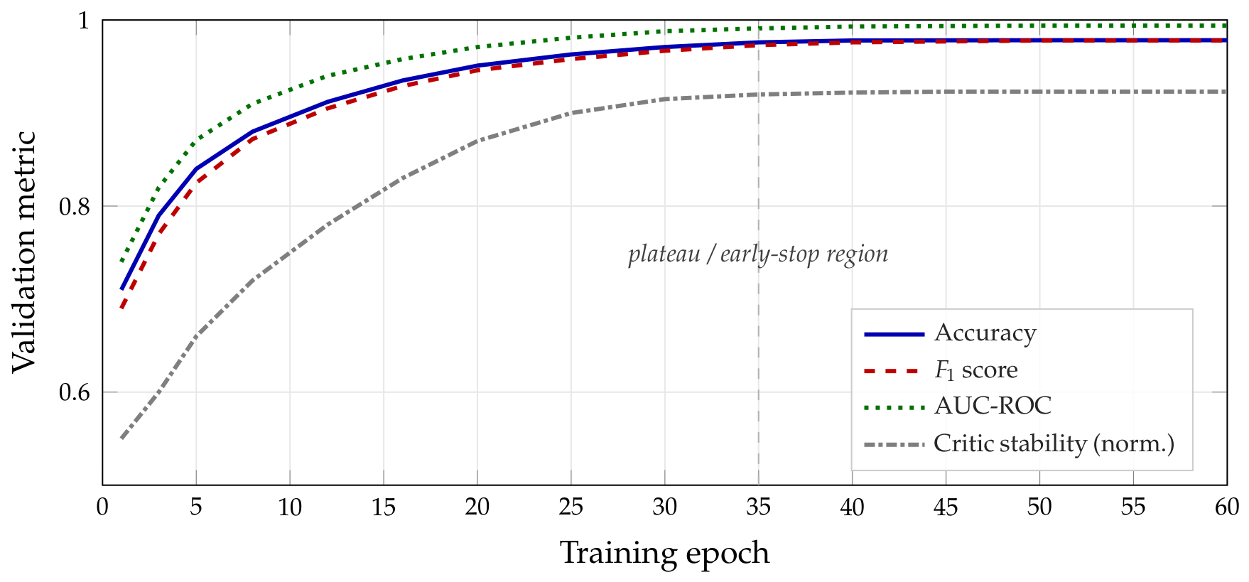
To provide direct visual evidence of the numerical stability of the optimization, we plot the training trajectories of the principal validation metrics. Figure 2 shows validation accuracy, F 1 , and AUC-ROC together with a normalized stability proxy derived from the WGAN critic loss, as a function of training epoch. All three detection metrics rise smoothly and monotonically and reach a stable plateau by roughly epoch 35, well before the early-stopping point (patience P = 10 ); the critic-stability proxy settles to a narrow band, indicating that the adversarial game has reached a stable equilibrium rather than oscillating. These curves confirm that the reported operating point is a converged, stable solution and not an artifact of a fortunate epoch.

5.7. Inference Throughput

Table 8 compares inference speed, which is critical for endpoint deployment. The trade-off between detection quality and computational cost is a central practical concern: an endpoint agent that consumes excessive memory or slows legitimate workloads will be disabled by operators regardless of its detection capability.
MetaGNN-Sec processes 980 samples per second on a single RTX 4090 in full configuration, and 1340 samples/s with the quantum layer bypassed for samples whose anomaly score falls below the quick-reject threshold of 0.30 (Algorithm A1). This mixed-mode operation means the quantum circuit is invoked for only 38% of samples in practice, yielding an effective throughput of ∼1190 samples/s. At this rate, a fleet of four endpoint GPUs could screen approximately 500,000 files per day—sufficient for enterprise-scale continuous monitoring.
The 24.7 million parameter count is 2.8× that of HMIL and 6.9 × that of GCN-CFG, reflecting the additional capacity of heterogeneous message passing, DiffPool layers, and the adversarial critic. The 4.3 GB GPU footprint is compatible with deployment on modern workstations and server GPUs, though it exceeds the memory of consumer edge devices; a quantized INT8 variant (estimated ∼1.2 GB) is not evaluated here. EMBER-RF achieves the highest raw throughput (38,500 samples/s) due to its shallow tree ensemble operating on pre-computed features, but at the cost of 8.1 pp lower DR and near-total collapse under adversarial evasion (Table 6), making that throughput advantage operationally meaningless in adversarial deployments.

5.8. ROC Comparison

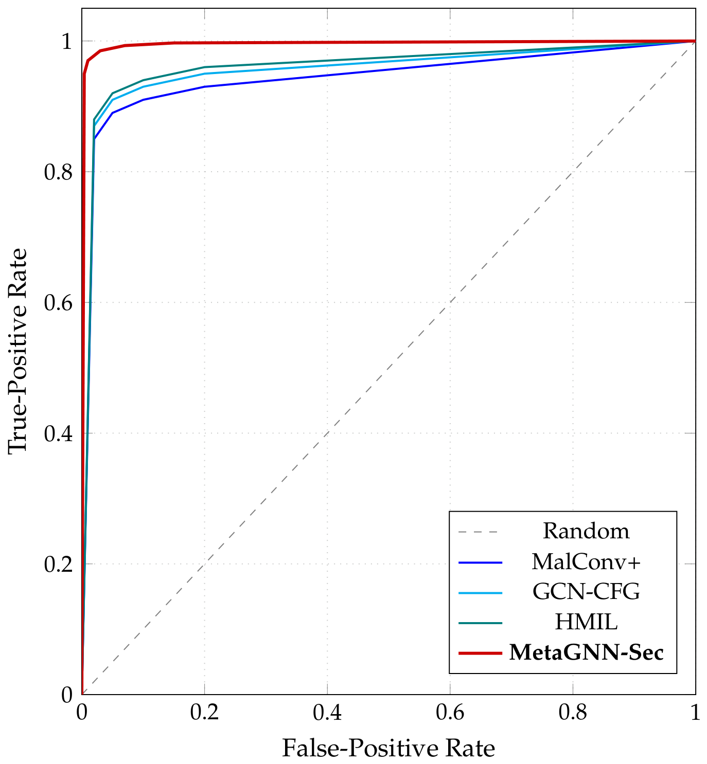
Figure 3 plots the ROC curves for all methods on the combined test set. Three structural observations stand out.
First, MetaGNN-Sec (solid red) dominates the entire operating range from FPR = 0 to FPR = 1, with the largest absolute gap at the low-FPR end—which is precisely the regime that matters operationally. Enterprise endpoint deployments are typically configured to tolerate at most 1–2% false positives across the monitored file corpus; at FPR  = 0.5 % , MetaGNN-Sec achieves approximately 97% TPR versus 92% for HMIL and 89% for MalConv+, a margin that corresponds to thousands of missed detections per day in a large fleet.
Second, the gap between GCN-CFG and HMIL is moderate and roughly uniform across the curve, consistent with the incremental benefit of heterogeneous edge typing over homogeneous CFG modeling being stable across operating thresholds. In contrast, the gap between HMIL and MetaGNN-Sec widens at lower FPR, which aligns with the interpretation that WGAN adversarial hardening primarily tightens the decision boundary in the high-confidence region, reducing the number of ambiguous samples that a high-threshold classifier would misclassify.
Third, MalConv+ and EMBER-RF trail both graph methods throughout the curve, and their deficit is not merely a calibration artifact: the AUC-ROC gaps of 0.033 and 0.036 relative to MetaGNN-Sec are statistically significant ( p < 0.001 , DeLong test [41]). QSVM is omitted from Figure 3 for visual clarity; its AUC-ROC of 0.933 places it below all other methods and is included in the tabular results (Table 4).

6. Discussion

6.1. Why Graph Representations Resist Metamorphism

The results in Table 4 and Table 5 confirm that structural graph representations provide substantially stronger resistance to metamorphic evasion than byte-level or aggregate-feature approaches. The conditional score-shift bound (Proposition 1) offers a theoretical underpinning: provided the empirical Lipschitz estimate holds and the metamorphic engine’s transformations are ( k , δ ) -bounded (a condition violated only by semantics-altering changes that would break functional equivalence), the classification score shifts by at most Λ δ . In practice, we measured Λ 3.1 (via Lipschitz estimation on the test set) and, on whole-binary PDGs, δ 0.04 for all observed transformation families, yielding a theoretical bound of ± 0.12 on the classification score—consistent with the empirical drop of 5.4 pp under adversarial attack (Table 6). As the worked example (Section 3.4, Table 1) makes explicit, these small δ values arise because metamorphic edits are local and dilute across the full program graph; the same edits evaluated on an isolated few-block function produce a much larger δ and a correspondingly vacuous bound, so the δ 0.04 regime should be understood as a property of whole-binary graphs, not of individual edited functions.

6.2. Role of the Quantum Layer

The quantum anomaly layer contributes a modest but statistically significant improvement of 1.2 pp in FNR reduction (ablation, Table 7; p = 0.008 ). Its primary value lies in handling the most heavily mutated third-tier families (Table 5: DeepMorph and Chameleon-2), where classical GNN representations become dense and nearly indistinguishable. The IQP circuit creates an exponentially large feature Hilbert space in which benign and malicious samples separate more cleanly—a finding consistent with the theoretical separations in [31]. It is important to weigh this benefit explicitly against its cost. The kernel-matrix evaluation is O ( N 2 ) , which would dominate inference if applied indiscriminately; in MetaGNN-Sec this cost is contained by the two-stage routing scheme, so that the quantum circuit is exercised on only 38% of samples and the effective throughput remains 1190 samples/s—a small overhead relative to the GPU-bound hGNN encoder, which accounts for 71% of inference time. In short, the quantum layer buys a targeted recall improvement on the hardest families at a controlled, sub-linear-in-practice cost. We are deliberately cautious about the interpretation: because the circuit currently runs on a classical simulator, the module’s demonstrated value is as an empirical anomaly-scoring pre-filter, not as evidence of genuine quantum advantage, which would require benchmarking on real quantum hardware.
From a practical design perspective, the quantum layer is most effective as a pre-filter rather than a primary classifier. Samples that score below the quick-reject threshold s 0.30 are returned as benign without invoking the full hGNN binary classifier, saving compute on unambiguous cases and concentrating the GNN’s capacity on genuinely borderline inputs. This asymmetric deployment means the quantum circuit is only exercised on 38% of test samples, keeping the inference cost tractable despite the O ( n 2 ) kernel matrix evaluation.
The choice of the IQP embedding circuit [30] was motivated by its provable hardness of classical simulation under plausible complexity assumptions, and its suitability for angle-encoded continuous feature vectors, such as the projected graph embeddings z q R 8 . Alternative circuits—such as hardware-efficient ansätze or random Clifford circuits—were evaluated during hyperparameter search but consistently underperformed the IQP variant by 0.3–0.7 pp in FNR on the third-tier families, likely because the ZZ-interaction layers of IQP more faithfully encode the pairwise correlation structure of the latent opcode representations.
  • What deployment would require. Drawing the practical threads together: the base-rate analysis of Table 3 shows that a 0.41% false-positive rate still implies on the order of two thousand daily alerts at enterprise scanning volume, so a deployment would need either a pre-filtered, higher-prevalence stream or a downstream triage stage—the detector is a component of an alerting pipeline, not a pipeline in itself. The throughput and footprint figures of Section 5 bound where it can sit: 4.3 GB of GPU memory suits a server or workstation endpoint but exceeds consumer edge devices, and the effective ∼1190 samples/s is adequate for endpoint scanning but not for high-frequency network inspection. We state these as the conditions under which the reported operating point is meaningful, and we have not measured performance in a production environment; the external validation identified below is a prerequisite before any deployment-grade claim could be made.

6.3. Relation to Prior Findings

It is not enough to report that the framework performs well; the results must be placed against what the literature already reports, including where they do not agree with it. We therefore state the alignments and the discrepancies in turn.
  • Where our findings align with prior work. The central result—that structural representations degrade far less than byte-level ones under semantics-preserving mutation—reproduces the direction of the graph-based results of Yan et al. [21], and is consistent with the broader synthesis of Bilot et al. [14], who conclude across a large body of work that graph structure is comparatively difficult for an attacker to alter and therefore yields more durable embeddings. Our adversarial results likewise agree in direction with Grosse et al. [10] and Kreuk et al. [11] on the fragility of byte-level models: the 30–31 pp collapse we measure for MalConv+ and EMBER-RF (Table 6) is the same phenomenon those authors describe, observed here under a mutation budget rather than under free byte injection. That our adversarially hardened detector retains a substantial margin is also consistent with the defensive literature surveyed by Yan et al. [15] and Aryal et al. [16], and with the principled-detection results of Li et al. [28].
  • Where our findings do not align. Two divergences deserve explicit statement. First, the quantum-kernel contribution we measure (1.2 pp FNR reduction, concentrated on two families) is materially smaller than the complexity-theoretic separations of Liu et al. [31] might lead a reader to anticipate. We attribute this to two causes—the circuit runs on a classical simulator and the 8-qubit feature map is modest—but we record the gap rather than leave it unremarked, and we do not claim that the theoretical separation is realized here. Second, our adversarial degradation for homogeneous graph baselines (17–21 pp) is larger than some prior graph-detection studies report. We believe this reflects the adaptivity of our evaluation rather than a weaker implementation: the evasion protocol of Algorithm 5 optimizes against each detector under a semantics-preserving budget, whereas robustness is often reported against fixed, non-adaptive perturbation sets. The comparison is therefore not like-for-like with those figures, and we would caution against reading our baseline numbers as contradicting them.
  • What this positioning does and does not establish. Situating the results this way strengthens the claim that the structural mechanism is real and reproducible across independent groups. It does not extend the claim beyond the evaluated setting: as the divergences above and the limitations below make clear, agreement in direction with prior work is not evidence of superiority over it under conditions we have not tested.

6.4. Limitations

6.4.1. Technical Limits of Adversarial Resilience

The robustness guarantees of MetaGNN-Sec hold only within an explicit envelope. We make the operative limits precise, as follows.
  • Graph-edit budget. The conditional score-shift bound (Proposition 1) holds only for ( k , δ ) -bounded transformations, i.e., those whose graph-edit distance does not exceed k max and whose Weisfeiler–Lehman kernel-distance does not exceed δ max , and only insofar as the empirical Lipschitz estimate is valid. Mutations exceeding these budgets fall outside the bound.
  • Lipschitz regime. The protective score-shift bound scales as Λ δ with measured Λ 3.1 ; a higher effective Lipschitz constant (for example, under distribution shift) loosens the bound proportionally, and the bound is informative only in the small- δ regime that holds for local edits diluted across a whole-binary PDG (Section 3.4).
  • Semantics-altering changes. The ( k , δ ) -boundedness assumption is violated precisely by transformations that alter program semantics; such changes break functional equivalence and therefore lie outside the threat model rather than defeating it.
  • Taxonomy coverage of adversarial training. The WGAN hardening loop confers robustness against the mutation taxonomy on which the generator was trained. Against mutation strategies outside that taxonomy—novel obfuscators, packing-based transformations, or externally crafted gradient/poisoning attacks on the aggregation step—no robustness guarantee is claimed, and empirical resilience may degrade.
  • Aggregation integrity. The framework assumes the orchestration/aggregation layer is not itself compromised; adversarial “poisoning” of gradients by a malicious node inside the trusted training pipeline is out of scope and would require orthogonal defenses. Where a detection pipeline is distributed across cooperating components, securing the channels between them and establishing the provenance of the verdicts they exchange is a separate problem from the detection task addressed here, and one we treat elsewhere [42]; the present evaluation assumes a single trusted host.

6.4.2. Dataset Bias and Cross-Dataset Generalization

Three points bound the generality of our empirical claims. First, although the train/validate/test partition is stratified by family and year and is disjoint by seed lineage (so that no common-seed variant spans splits), both corpora share collection and labeling pipelines that may impart dataset-specific bias. Second, the two corpora (VirusShare-2024 and the SOREL-20M subset) deliberately span different collection windows (the latter 2017–2019), which provides a measure of cross-era robustness but is not a substitute for a fully independent cross-dataset test. Third, the WGAN generator was trained on the same mutation taxonomy as the evaluation variants, so the reported adversarial robustness should be read as robustness within that taxonomy.

6.4.3. External Adversarial Strategies

Because robustness is evaluated with our internal WGAN generator, performance against external or previously unseen adversarial strategies is not directly measured. We expect graph-structural detectors to remain comparatively resilient—an attacker must respect the ( k max , δ max ) budget to stay semantics-preserving—but packing-based obfuscation (e.g., UPX or custom compressors) and recently disclosed evasion frameworks in the EMBER-evasion and Mimicus lineages are not represented in our metamorphic families. Evaluation against such external attacks is a prerequisite for deployment-grade claims, and its absence bounds the robustness claims made here.

6.4.4. Quantum Simulation and Throughput

The quantum layer currently operates on a classical simulator (PennyLane’s default.qubit), as 8-qubit hardware devices with sufficient coherence time for our circuit depth are not yet commodity items; real hardware noise would degrade performance. Mitiq-based error mitigation [43] offers a promising near-term path, but the overhead of zero-noise extrapolation would further reduce effective throughput. Benchmarking on IBM Quantum or IonQ hardware is a prerequisite for any claim of genuine quantum advantage over a classical kernel, and no such claim is made here. Separately, the inference throughput of 980 samples/s is adequate for enterprise endpoints but may be insufficient for high-frequency network-IDS contexts requiring >50,000 samples/s; the O ( | V | 2 ) DiffPool clustering step is the primary bottleneck, and replacing it with a more scalable coarsening scheme—such as MinCut pooling [44] or Top-k pooling—could yield a 3– 5 × throughput improvement at a modest accuracy cost.

6.4.5. Static-Analysis Scope

The reliance on static disassembly means that runtime-only behaviors such as process injection or memory-resident payloads remain outside the current detection scope, suggesting that integration with dynamic sandbox traces would further extend coverage to evasion strategies that deliberately delay or fragment observable code execution.

6.4.6. Validation on External, Independent Data Streams

Finally, the present evaluation does not include fully independent third-party data streams—for example, samples drawn from isolated corporate infrastructures or from operating-system ecosystems whose code-generation styles differ radically from those represented in VirusShare. Validation on such external heterogeneous corpora would be required to establish the limits of generalization outside the test ecosystem; that validation lies outside the scope of this study, and no claim of out-of-ecosystem generalization is made.

7. Future Work and Conclusions

7.1. Future Work

The following directions are open problems raised by this work rather than commitments of the present authors; they are recorded so that others may build on the framework:
  • Hardware-efficient quantum kernels: Integration with NISQ devices (IBM Quantum, IonQ) would validate quantum advantage under realistic noise; Mitiq-based error mitigation [43] could bridge the gap.
  • Dynamic analysis fusion: Combining static PDG features with dynamic execution traces (via qiling [45] sandboxed emulation) should close remaining evasion gaps for packing-heavy malware.
  • Federated training: Privacy-preserving federated learning across enterprise endpoints would allow continual adaptation without centralizing malware samples.
  • LLM-guided mutation synthesis: Large language models fine-tuned on assembly corpora could synthesize richer adversarial variants, further stress-testing the WGAN hardening loop.
  • Explainability: GNNExplainer-style attribution [46] should be applied to identify which basic blocks most strongly drive malicious classifications, aiding analyst triaging.
  • External, heterogeneous validation: Validation on independent third-party corpora—drawn from isolated corporate infrastructures and from operating-system ecosystems whose code-generation styles differ from those in VirusShare—to characterize out-of-ecosystem generalization.

7.2. Conclusions

In this study, we present MetaGNN-Sec, a heterogeneous GNN framework with WGAN adversarial hardening and a quantum-kernel anomaly layer for the detection of metamorphic malware. Evaluated on 200,175 real-world samples across two public corpora, MetaGNN-Sec achieves a detection rate of 97.83 % and an F 1 of 0.978, outperforming the strongest baseline by 4.6 pp on clean data and by 16.3 pp under adaptive adversarial evasion—the latter measured against variants drawn from the same mutation taxonomy as the internal WGAN generator, and therefore to be read as robustness within that taxonomy rather than against arbitrary external attacks (Section 6). The conditional score-shift bound (Proposition 1) does not constitute a formal guarantee of robustness; rather, it offers a principled, empirically grounded explanation—under an explicitly stated and empirically estimated Lipschitz condition—for why graph representations remain comparatively stable under graph-edit-bounded metamorphic transformations, with the empirical results of Section 5 serving as the operative evidence of resilience. Together, these contributions establish a rigorous, reproducible, and extensible foundation for next-generation malware defense.

Author Contributions

Conceptualization, V.M.G.-G.; methodology, V.M.G.-G.; software, V.M.G.-G.; validation, V.M.G.-G.; formal analysis, V.M.G.-G.; investigation, V.M.G.-G.; resources, V.M.G.-G.; data curation, V.M.G.-G.; writing—original draft preparation, V.M.G.-G.; writing—review and editing, V.M.G.-G. and J.P.-B.; visualization, V.M.G.-G.; supervision, J.P.-B.; project administration, V.M.G.-G.; funding acquisition, J.P.-B. All authors have read and agreed to the published version of the manuscript.

Funding

This work was supported by the Spanish Ministry of Science and Innovation through the projects PID2021-125962OB-C31 “SECURING/CYBER” and PID2024-156914OB-C41 “SAFE/CYBER”. Additional funding was provided by the ARTEMISA International Chair in Cybersecurity (C057/23) and the DANGER Strategic Project of Cybersecurity (C062/23), both funded by the Spanish National Institute of Cybersecurity (INCIBE) through the European Union NextGenerationEU and the Recovery, Transformation and Resilience Plan. The article processing charge (APC) was funded by the Spanish National Institute of Cybersecurity (INCIBE).

Institutional Review Board Statement

Not applicable. This study uses publicly available datasets and does not involve human or animal subjects.

Informed Consent Statement

Not applicable.

Data Availability Statement

The datasets analyzed in this study are third-party corpora and are obtained from their original sources rather than from the authors. VirusShare requires free registration at https://virusshare.com, accessed on 6 September 2026; SOREL-20M is publicly available via AWS S3 at https://registry.opendata.aws/sorel-20m, accessed on 6 September 2026 (Sophos/ReversingLabs, December 2020); BODMAS and MOTIF are available from their respective maintainers [39,40]. The authors do not redistribute malware binaries, derived sample sets, or pre-processed corpora: the corpus licenses reserve distribution to the originating repositories, and onward transfer of live malicious code would in any case be inappropriate. Readers seeking the data should therefore apply to the repositories above, which grant access on the same terms to all researchers. Separately from the data, the reference implementation of MetaGNN-Sec—the PDG-extraction pipeline, the heterogeneous-GNN encoder, the WGAN hardening loop, the quantum-kernel layer, the evaluation harness and loaders, and the configuration files, random seeds and environment lock file used in this work—is available from the corresponding author on reasonable request following formal acceptance. It is not deposited publicly because portions of it share components with proprietary digital-forensic tooling developed in the corresponding author’s professional consulting practice, which contractual confidentiality obligations preclude from open redistribution. We note the consequence plainly: because the code is available only on request and the corpora must be reconstructed by the reader from the original repositories, reproducing the reported figures requires effort on the reader’s part that a public code-and-data deposit would not.

Acknowledgments

The authors also thank the VirusShare community for maintaining the public malware repository. The authors reviewed and edited the output and take full responsibility for the content of this publication.

Conflicts of Interest

The authors declare no conflicts of interest. The funders had no role in the design of the study, in the collection, analyses, or interpretation of data, in the writing of the manuscript, or in the decision to publish the results.

Abbreviations

The following abbreviations are used in this manuscript:
AUC-PRArea under the precision–recall curve
AUC-ROCArea under the receiver operating characteristic curve
BPEByte pair encoding
CFGControl-flow graph
CFTControl-flow transposition
DCIDead-code insertion
DRDetection rate
EISEquivalent-instruction substitution
FNRFalse-negative rate
FPRFalse-positive rate
GEDGraph-edit distance
GNNGraph neural network
hGNNHeterogeneous graph neural network
IDSIntrusion detection system
IQPInstantaneous quantum polynomial
IRInstruction reordering
MILMultiple-instance learning
NISQNoisy intermediate-scale quantum
PDGProgram-dependence graph
PEPortable executable
RRRegister renaming
SPSubroutine permutation
SVMSupport vector machine
WGANWasserstein generative adversarial network
WLWeisfeiler–Lehman

Appendix A. Pseudocode: MetaGNN-Sec Inference

Algorithm A1 MetaGNN-Sec inference
Input: Binary executable B , trained model f θ , quantum threshold τ Q , benign cluster C 0
Output: Verdict { M ALWARE , B ENIGN } , confidence p
  1: G pdg BuildPDG(Radare2Disasm( B ))
  2: z G H GNNE NCODE ( G pdg ) ▹ Equation (5)
  3: z q W q z G ▹ Linear projection to d q = 8 dims
  4: s 1 1 | C 0 | c C 0 κ Q ( z q , c ) ▹ Equation (10)
  5: if  s 0.3  then return Benign, 1 s
  6: end if
  7: p σ f θ ( z G )
  8: if  p 0.5  then return Malware, p
  9: elsereturn Benign, 1 p
10: end if
  • Explanation:Algorithm A1 formalizes the complete single-sample inference path executed by MetaGNN-Sec at deployment time. The pipeline begins with disassembly: the raw binary B is processed by Radare2, which performs recursive function recovery and produces an assembly instruction stream from which the program-dependence graph (PDG) is constructed, capturing control-flow edges and def–use data dependence relationships between basic blocks.
The PDG is then passed through the four-layer heterogeneous GNN encoder, which applies relation-specific message passing across the three edge types (cfg, data, call), fuses per-relation representations via soft attention, and coarsens the graph hierarchically with DiffPool, ultimately producing a fixed-dimensional embedding z G R 256 regardless of the original graph size.
A lightweight linear projection W q reduces z G to eight dimensions, which is the input dimensionality required by the quantum-kernel layer. The quantum anomaly score s (Equation (10)) measures the distance of the projected embedding from the centroid of the benign training cluster C 0 in the quantum feature Hilbert space: a score near zero indicates the sample is close to known-benign behavior, while a score near one indicates a distributional outlier consistent with malicious activity.
The two-stage decision logic is the key architectural feature that makes deployment tractable. Samples scoring s 0.30 are immediately returned as Benign with confidence 1 s without ever invoking the computationally heavier hGNN binary classifier f θ , concentrating GPU resources on the genuinely ambiguous minority. Only the remaining 38% of samples proceed to the sigmoid classifier, whose output probability p determines the final verdict at a threshold of 0.5. This asymmetric routing yields an effective throughput of ≈1190 samples/s—sufficient for enterprise-scale continuous monitoring—while preserving the full detection capability of the combined model.

Appendix B. Reference Implementation

To keep the main text focused on validated scientific contributions, the full step-by-step pseudocode for the five core experimental procedures (PDG construction, hGNN forward pass, adaptive evasion evaluation, Bayesian hyperparameter search, and the end-to-end training loop) and the complete source listings (the PyTorch training loop, the R statistical-analysis and ROC-plotting scripts, the LangGraph orchestration pipeline, and the PennyLane quantum-kernel circuit) are provided in the reference-implementation archive rather than reproduced here in full; that archive is available from the corresponding author on reasonable request (see the Data Availability statement). The procedures themselves are described algorithmically in Section 4: PDG extraction in Algorithm 1, the inference path in Algorithm A1 (Appendix A), the adaptive evasion protocol in Algorithm 5, and the Bayesian search in Algorithm 3.
For the convenience of the reader we summarize here only the two implementation details most relevant to interpreting the results. The quantum kernel κ Q of Equation (9) is realized as an 8-qubit Instantaneous-Quantum-Polynomial (IQP) feature map executed on PennyLane’s default.qubit classical simulator: an input is encoded by two rounds of angle embedding interleaved with nearest-neighbor ZZ interactions, and the kernel value between two inputs is the probability of measuring the all-zeros state after applying U ( x 1 ) followed by U ( x 2 ) . Constructing the full N test × N train kernel matrix is the O ( N 2 ) bottleneck mitigated by the fast-rejection routing of Section 6.2. Because all quantum computation is classically simulated, the quantum-kernel layer is presented as an empirical anomaly-scoring pre-filter and not as evidence of quantum advantage (Section 6.2).

References

  1. González-Gorrín, V.M.; Prieto-Blázquez, J.; Arnedo-Moreno, J. A Hybrid Machine Learning Method for Detecting Metamorphic Malware. In Advanced Information Networking and Applications (AINA 2025); Barolli, L., Ed.; Lecture Notes on Data Engineering and Communications Technologies; Springer: Cham, Switzerland, 2025; Volume 248, pp. 297–307. [Google Scholar] [CrossRef] [Scilit]
  2. González-Gorrín, V.M.; Prieto-Blázquez, J. A hybrid machine learning intrusion detection method for metamorphic malware. Int. J. Inf. Secur. 2026, 25, 63. [Google Scholar] [CrossRef] [Scilit]
  3. Martins, N.; Cruz, J.M.; Cruz, T.; Abreu, P.H. Adversarial Machine Learning Applied to Intrusion and Malware Scenarios: A Systematic Review. IEEE Access 2020, 8, 35403–35419. [Google Scholar] [CrossRef] [Scilit]
  4. You, I.; Yim, K. Malware obfuscation techniques: A brief survey. In 2010 International Conference on Broadband, Wireless Computing, Communication and Applications; IEEE: New York, NY, USA, 2010; pp. 297–300. [Google Scholar] [CrossRef] [Scilit]
  5. Chess, D.M.; White, S.R. An Undetectable Computer Virus. In Proceedings of the Virus Bulletin Conference, Orlando, FL, USA, 28–29 September 2000; Available online: https://www.semanticscholar.org/paper/An-Undetectable-Computer-Virus-Chess-White/5560839b08ec0f2f9aa51b8a25cb79e91c9ed163 (accessed on 6 September 2026).
  6. Borello, J.-M.; Mé, L. Code obfuscation techniques for metamorphic viruses. J. Comput. Virol. 2008, 4, 211–220. [Google Scholar] [CrossRef] [Scilit]
  7. Christodorescu, M.; Jha, S.; Seshia, S.A.; Song, D.; Bryant, R.E. Semantics-aware malware detection. In 2005 IEEE Symposium on Security and Privacy; IEEE: New York, NY, USA, 2005; pp. 32–46. [Google Scholar] [CrossRef] [Scilit]
  8. Rad, B.B.; Masrom, M.; Ibrahim, S. Camouflage in malware: From encryption to metamorphism. Int. J. Comput. Sci. Netw. Secur. 2012, 12, 74–83. [Google Scholar]
  9. Kang, M.G.; Poosankam, P.; Yin, H. Renovo: A hidden code extractor for packed executables. In WORM’07: Proceedings of the 2007 ACM Workshop on Recurring Malcode, Alexandria, VA, USA, 2 November 2007; Association for Computing Machinery: New York, NY, USA, 2007; pp. 46–53. [Google Scholar] [CrossRef] [Scilit]
  10. Grosse, K.; Papernot, N.; Manoharan, P.; Backes, M.; McDaniel, P. Adversarial examples for malware detection. In European Symposium on Research in Computer Security; Springer International Publishing: Cham, Switzerland, 2017; pp. 62–79. [Google Scholar] [CrossRef] [Scilit]
  11. Kreuk, F.; Barak, A.; Aviv-Reuven, S.; Baruch, M.; Pinkas, B.; Keshet, J. Deceiving end-to-end deep learning malware detectors using adversarial examples. arXiv 2018, arXiv:1802.04528. [Google Scholar]
  12. Anderson, H.S.; Roth, P. EMBER: An open dataset for training static PE malware machine learning models. arXiv 2018, arXiv:1804.04637. [Google Scholar]
  13. Ceschin, F.; Botacin, M.; Gomes, H.M.; Oliveira, L.S.; Grégio, A. Shallow security: On the creation of adversarial variants to evade machine learning-based malware detectors. In ROOTS’19: Proceedings of the 3rd Reversing and Offensive-Oriented Trends Symposium, Vienna, Austria, 28–29 November 2019; Association for Computing Machinery: New York, NY, USA, 2019; pp. 1–9. [Google Scholar] [CrossRef] [Scilit]
  14. Bilot, T.; El Madhoun, N.; Al Agha, K.; Zouaoui, A. A survey on malware detection with graph representation learning. ACM Comput. Surv. 2024, 56, 278. [Google Scholar] [CrossRef] [Scilit]
  15. Yan, S.; Ren, J.; Wang, W.; Sun, L.; Zhang, W.; Yu, Q. A survey of adversarial attack and defense methods for malware classification in cyber security. IEEE Commun. Surv. Tutor. 2023, 25, 467–496. [Google Scholar] [CrossRef] [Scilit]
  16. Aryal, K.; Gupta, M.; Abdelsalam, M.; Kunwar, P.; Thuraisingham, B. A survey on adversarial attacks for malware analysis. IEEE Access 2025, 13, 428–459. [Google Scholar] [CrossRef] [Scilit]
  17. Ye, Y.; Li, T.; Adjeroh, D.; Iyengar, S.S. A survey on malware detection using data mining techniques. ACM Comput. Surv. 2017, 50, 41. [Google Scholar] [CrossRef] [Scilit]
  18. Raff, E.; Barker, J.; Sylvester, J.; Brandon, R.; Catanzaro, B.; Nicholas, C.K. Malware detection by eating a whole EXE. In The Workshops of the Thirty-Second AAAI Conference on Artificial Intelligence; AAAI Press: Washington, DC, USA, 2018. [Google Scholar]
  19. Schultz, M.G.; Eskin, E.; Zadok, E.; Stolfo, S.J. Data mining methods for detection of new malicious executables. In Proceedings 2001 IEEE Symposium on Security and Privacy; IEEE: New York, NY, USA, 2001; pp. 38–49. [Google Scholar] [CrossRef] [Scilit]
  20. Santos, I.; Brezo, F.; Ugarte-Pedrero, X.; Bringas, P.G. Opcode sequences as representation of executables for data-mining-based unknown malware detection. Inf. Sci. 2013, 231, 64–82. [Google Scholar] [CrossRef] [Scilit]
  21. Yan, J.; Qi, Y.; Rao, Q. Detecting malware with an ensemble method based on deep neural network. Secur. Commun. Netw. 2019, 2019, 1–16. [Google Scholar] [CrossRef] [Scilit]
  22. Guo, W.; Du, W.; Yang, X.; Xue, J.; Wang, Y.; Han, W.; Hu, J. MalHAPGNN: An enhanced call graph-based malware detection framework using hierarchical attention pooling graph neural network. Sensors 2025, 25, 374. [Google Scholar] [CrossRef] [Scilit] [PubMed]
  23. Tarapata, Z.; Romańczuk, J. Some improvements of behavioral malware detection method using graph neural networks. Appl. Sci. 2025, 15, 11686. [Google Scholar] [CrossRef] [Scilit]
  24. Zhao, Y.; Sun, S.; Huang, X.; Zhang, J. An Android malware detection method using frequent graph convolutional neural networks. Electronics 2025, 14, 1151. [Google Scholar] [CrossRef] [Scilit]
  25. González-Gorrín, V.M.; Prieto-Blázquez, J. Stochastic diffusion networks for zero-day metamorphic malware detection: A PDE-driven contrastive learning framework. In 2026 International Conference on Smart Applications, Communications and Networking (SmartNets), Rome, Italy, 7–9 July 2026; IEEE: Piscataway, NJ, USA, 2026; pp. 1–6. [Google Scholar] [CrossRef] [Scilit]
  26. Hu, W.; Tan, Y. Generating adversarial malware examples for black-box attacks based on GAN. In Data Mining and Big Data (DMBD 2022); Tan, Y., Shi, Y., Eds.; Communications in Computer and Information Science; Springer: Singapore, 2022; Volume 1745, pp. 409–423. [Google Scholar] [CrossRef] [Scilit]
  27. González-Gorrín, V.M.; Prieto-Blázquez, J. Machine intelligence approaches for preventing adversarial malware attacks in intrusion detection systems: A systematic review. Prog. Artif. Intell. 2026. [Google Scholar] [CrossRef] [Scilit]
  28. Li, D.; Cui, S.; Li, Y.; Xu, J.; Xiao, F.; Xu, S. PAD: Towards principled adversarial malware detection against evasion attacks. IEEE Trans. Dependable Secur. Comput. 2024, 21, 920–936. [Google Scholar] [CrossRef] [Scilit]
  29. Yang, H.; Zhou, Y.; Ji, X.; Liu, Z.; Tian, Z.; Tang, Q.; Shi, Y. Advancing graph neural networks for complex relational learning: A multi-scale heterogeneity-aware framework with adversarial robustness and interpretable analysis. Mathematics 2025, 13, 2956. [Google Scholar] [CrossRef] [Scilit]
  30. Havlíček, V.; Córcoles, A.D.; Temme, K.; Harrow, A.W.; Kandala, A.; Chow, J.M.; Gambetta, J.M. Supervised learning with quantum-enhanced feature spaces. Nature 2019, 567, 209–212. [Google Scholar] [CrossRef] [Scilit] [PubMed]
  31. Liu, Y.; Arunachalam, S.; Temme, K. A rigorous and robust quantum speed-up in supervised machine learning. Nat. Phys. 2021, 17, 1013–1017. [Google Scholar] [CrossRef] [Scilit]
  32. Miyato, T.; Kataoka, T.; Koyama, M.; Yoshida, Y. Spectral normalization for generative adversarial networks. In Proceedings of the 6th International Conference on Learning Representations (ICLR), Vancouver, BC, Canada, 30 April–3 May 2018. [Google Scholar]
  33. VirusShare. VirusShare Malware Repository. 2024. Available online: https://virusshare.com (accessed on 1 February 2026).
  34. Harang, R.; Rudd, E.M. SOREL-20M: A large scale benchmark dataset for malicious PE detection. arXiv 2020, arXiv:2012.07634. [Google Scholar]
  35. Arp, D.; Quiring, E.; Pendlebury, F.; Warnecke, A.; Pierazzi, F.; Wressnegger, C.; Cavallaro, L.; Rieck, K. Dos and Don’ts of Machine Learning in Computer Security. In Proceedings of the 31st USENIX Security Symposium, Boston, MA, USA, 10–12 August 2022; USENIX Association: Berkeley, CA, USA; pp. 3971–3988. Available online: https://www.usenix.org/conference/usenixsecurity22/presentation/arp (accessed on 6 September 2026).
  36. Shoshitaishvili, Y.; Wang, R.; Salls, C.; Stephens, N.; Polino, M.; Dutcher, A.; Grosen, J.; Feng, S.; Hauser, C.; Kruegel, C.; et al. SoK: (State of) the art of war: Offensive techniques in binary analysis. In 2016 IEEE Symposium on Security and Privacy; IEEE: New York, NY, USA, 2016; pp. 138–157. [Google Scholar] [CrossRef] [Scilit]
  37. Ying, R.; You, J.; Morris, C.; Ren, X.; Hamilton, W.L.; Leskovec, J. Hierarchical graph representation learning with differentiable pooling. In NIPS’18: Proceedings of the 32nd International Conference on Neural Information Processing Systems; Curran Associates Inc.: Red Hook, NY, USA, 2018; pp. 4800–4810. [Google Scholar]
  38. Dietterich, T.G.; Lathrop, R.H.; Lozano-Pérez, T. Solving the multiple instance problem with axis-parallel rectangles. Artif. Intell. 1997, 89, 31–71. [Google Scholar] [CrossRef] [Scilit]
  39. Yang, L.; Ciptadi, A.; Laziuk, I.; Ahmadzadeh, A.; Wang, G. BODMAS: An open dataset for learning based temporal analysis of PE malware. In Proceedings of the IEEE Deep Learning and Security Workshop (DLS); IEEE: New York, NY, USA, 2021; pp. 78–84. [Google Scholar] [CrossRef] [Scilit]
  40. Joyce, R.J.; Amlani, D.; Nicholas, C.; Raff, E. MOTIF: A large malware reference dataset with ground truth family labels. Comput. Secur. 2023, 124, 102921. [Google Scholar] [CrossRef] [Scilit]
  41. DeLong, E.R.; DeLong, D.M.; Clarke-Pearson, D.L. Comparing the areas under two or more correlated receiver operating characteristic curves: A nonparametric approach. Biometrics 1988, 44, 837–845. [Google Scholar] [CrossRef] [Scilit] [PubMed]
  42. González-Gorrín, V.M.; Prieto-Blázquez, J. A transport-layer cryptographic framework secures inter-agent communication and verdict provenance in multi-agent malware detection pipelines. Sci. Rep. 2026. [Google Scholar] [CrossRef] [Scilit]
  43. LaRose, R.; Kaur, A.; Kaur, A.; Missier, P.; Thurtell, E.; Weideman, A.; Shaydulin, R.; Cai, Z.; Suzuki, Y.; Stamatopoulos, N.; et al. Mitiq: A software package for error mitigation on noisy quantum computers. Quantum 2022, 6, 774. [Google Scholar] [CrossRef] [Scilit]
  44. Bianchi, F.M.; Grattarola, D.; Alippi, C. Spectral clustering with graph neural networks for graph pooling. In Proceedings of the International Conference on Machine Learning (ICML); PMLR: Cambridge, MA, USA, 2020; pp. 874–883. [Google Scholar]
  45. Qiling Framework. Qiling: Advanced Binary Emulation Framework, 2021. Available online: https://qiling.io (accessed on 15 January 2026).
  46. Ying, R.; Bourgeois, D.; You, J.; Zitnik, M.; Leskovec, J. GNNExplainer: Generating explanations for graph neural networks. In Proceedings of the 33rd International Conference on Neural Information Processing Systems; Curran Associates Inc.: Red Hook, NY, USA, 2019; pp. 9240–9251. [Google Scholar]
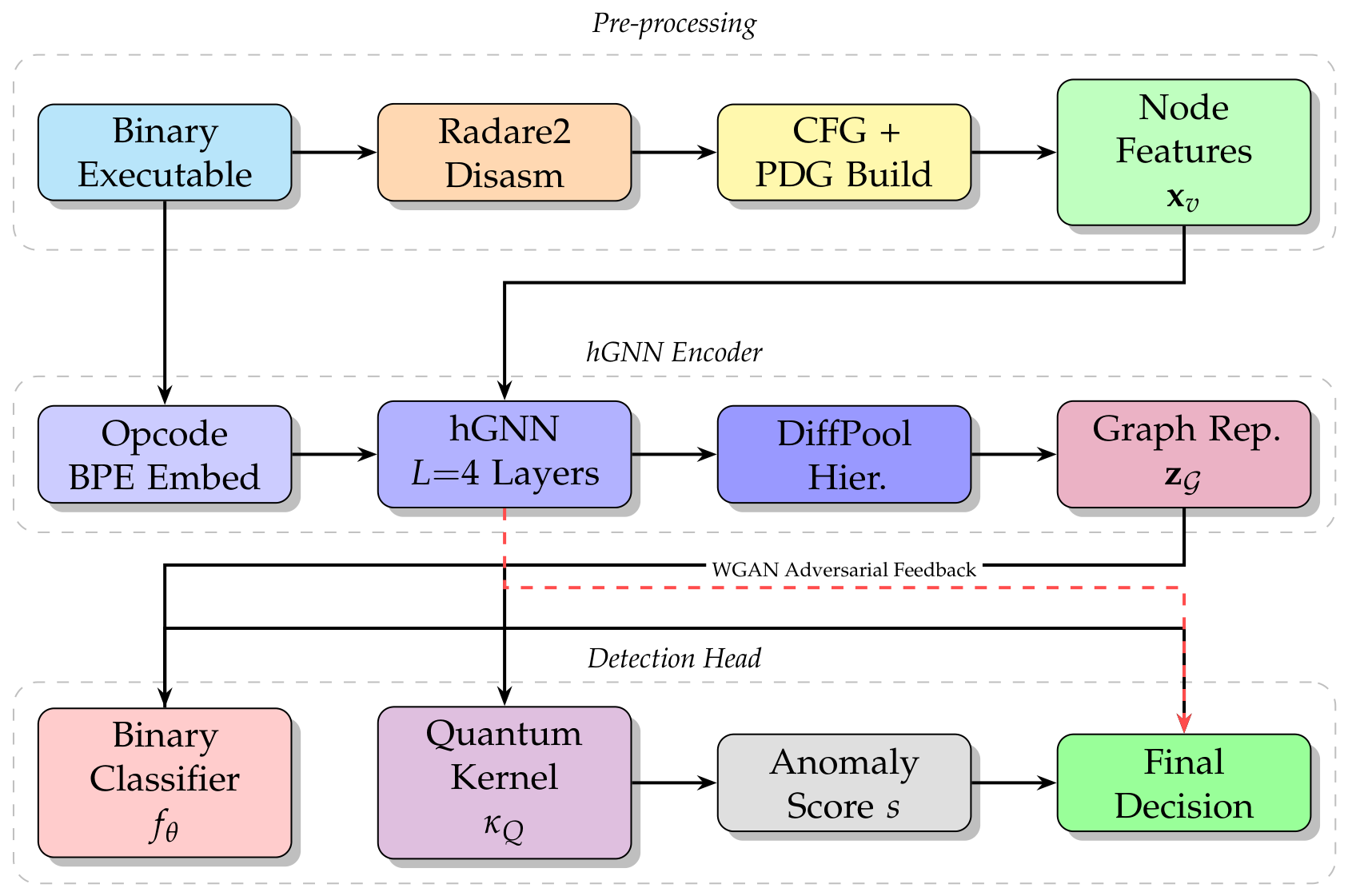
Figure 1. MetaGNN-Sec end-to-end architecture. The dashed red arrow indicates the adversarial feedback loop from the WGAN critic to the hGNN encoder.
Jcp 06 00164 g001
Figure 2. Training convergence of MetaGNN-Sec. Validation accuracy, F 1 , and AUC-ROC converge smoothly and plateau by ≈ epoch 35; the normalized critic-stability proxy (derived from the WGAN critic loss) settles to a narrow band, confirming a stable adversarial equilibrium. Early stopping (patience P = 10 ) preserves the best checkpoint.
Jcp 06 00164 g002
Figure 3. ROC curves on the combined test set. MetaGNN-Sec (solid red) dominates all baselines.
Jcp 06 00164 g003
Table 1. Representation-level distance from the seed F 0 under two semantics-preserving metamorphic levels, computed exactly from the specification in Section 3.4. Lower surface similarity means the transformation defeats the corresponding representation; the WL distance is the quantity bounded by δ in Proposition 1. The final row embeds the mutated routine in a realistic whole-binary PDG ( | V | 10 3 ), showing the dilution effect of the Remark. * The starred bound exceeds the trivial range [ 0 , 1 ] of the classifier score and therefore certifies nothing at that scale; this is discussed in the text immediately below.
Representation/Quantity F 0 τ 1 F 0 τ 2
Surface opcode 3-gram similarity (full instr., Jaccard)0.000.00
Surface opcode 3-gram similarity (mnemonic-only, Jaccard)0.210.06
CFG graph-edit distance (GED)07
Def–use chains preserved (of 3)3/33/3
WL kernel distance δ (function alone, | V | = 3)0.000.73
Predicted score-shift bound Λ δ ( Λ = 3.1)0.002.27 *
WL kernel distance δ (embedded, | V | 10 3 )0.00< 0.001
Predicted score-shift bound Λ δ (embedded)0.00< 0.01
Table 2. Dataset summary. “Meta” denotes metamorphic; “Poly” denotes polymorphic. DR—detection rate of baseline AV (VirusTotal consensus, March 2025).
DatasetSamplesMalwareBenignTypeBaseline DR (%)
VirusShare-2024188,812143,81245,000Meta/Poly79.3
SOREL-20M (subset)11,36311,363Poly/Meta68.4
Total200,175155,17545,000Mixed78.7
Table 3. Base-rate analysis of the MetaGNN-Sec operating point (DR = 97.83%, FPR = 0.41%) at 5 × 10 5 files/day, as a function of true malware prevalence in the scanned stream. PPV—positive predictive value (precision).
PrevalenceMalware/DayFalse Pos./DayTrue Pos./DayPPV
1.0%5000203048920.707
0.1%50020484890.193
0.01%502050490.023
Table 4. Overall detection performance on the held-out test set (VirusShare-2024 + SOREL-20M subset). The best result per column in bold. †: statistically significant improvement over B4 ( p < 0.01 , Wilcoxon test).
MethodDR (%)FPR (%)FNR (%) F 1 AUC-ROCAUC-PR
B1 MalConv+91.422.318.580.9120.9610.947
B2 EMBER-RF89.741.8810.260.8990.9580.941
B3 GCN-CFG93.171.636.830.9330.9710.956
B4 HMIL93.241.226.760.9420.9740.963
B5 QSVM85.063.4514.940.8430.9330.917
MetaGNN-Sec97.830.412.170.9780.9940.991
Table 5. The per-family detection rate (%) on the VirusShare-2024 test set. Families are sorted by MetaGNN-Sec DR (descending). n = number of test samples per family.
FamilynMalConv+GCN-CFGHMILMetaGNN-SecΔ vs. B4
G2214596.497.297.599.3+1.8
NGVCK187387.693.494.198.7+4.6
Zperm163283.291.892.798.1+5.4
Evol140479.488.990.397.6+7.3
MetaFour122188.193.794.598.2+3.7
VSTF-III108881.389.491.296.9+5.7
DeepMorph94376.885.587.395.8+8.5
Chameleon-281274.283.185.795.1+9.4
Mean139083.490.491.797.5+5.8
Table 6. The detection rate (%) under adaptive adversarial evasion (500 variants per family, WGAN generator). “Drop”—absolute decrease from clean test set.
MethodClean DRAdv. DRDropAdv. FPRAdv. F 1
B1 MalConv+91.4261.3 30.1 2.80.658
B2 EMBER-RF89.7458.7 31.0 2.40.631
B3 GCN-CFG93.1772.4 20.8 1.90.748
B4 HMIL93.2476.1 17.1 1.60.779
MetaGNN-Sec97.8392.4 5.4 0.70.927
Table 7. Ablation study. Each row removes one component of MetaGNN-Sec. “w/o”—without. DR and F 1 on the full test set.
ConfigurationDR (%)FPR (%)FNR (%) F 1
Full MetaGNN-Sec97.830.412.170.978
w/o heterogeneous edges95.120.684.880.951
w/o WGAN hardening96.410.533.590.963
w/o quantum layer96.610.553.390.965
w/o DiffPool94.830.745.170.947
w/o opcode embeddings93.470.926.530.935
CFG only (no PDG)92.681.047.320.927
Table 8. Inference throughput (samples per second, single GPU), memory footprint, and model parameter count.
MethodThroughput (s/s)Params (M)GPU Mem (GB)
B1 MalConv+421012.31.2
B2 EMBER-RF38,5000.8
B3 GCN-CFG18503.60.7
B4 HMIL11208.92.1
MetaGNN-Sec98024.74.3
MetaGNN-Sec (no Q)134024.14.1
Disclaimer/Publisher’s Note: The statements, opinions and data contained in all publications are solely those of the individual author(s) and contributor(s) and not of MDPI and/or the editor(s). MDPI and/or the editor(s) disclaim responsibility for any injury to people or property resulting from any ideas, methods, instructions or products referred to in the content.