
Detecting Jamming in Smart Grid Communications via Deep Learning

 ,
,  ,
,  and
and
Abstract
1. Introduction
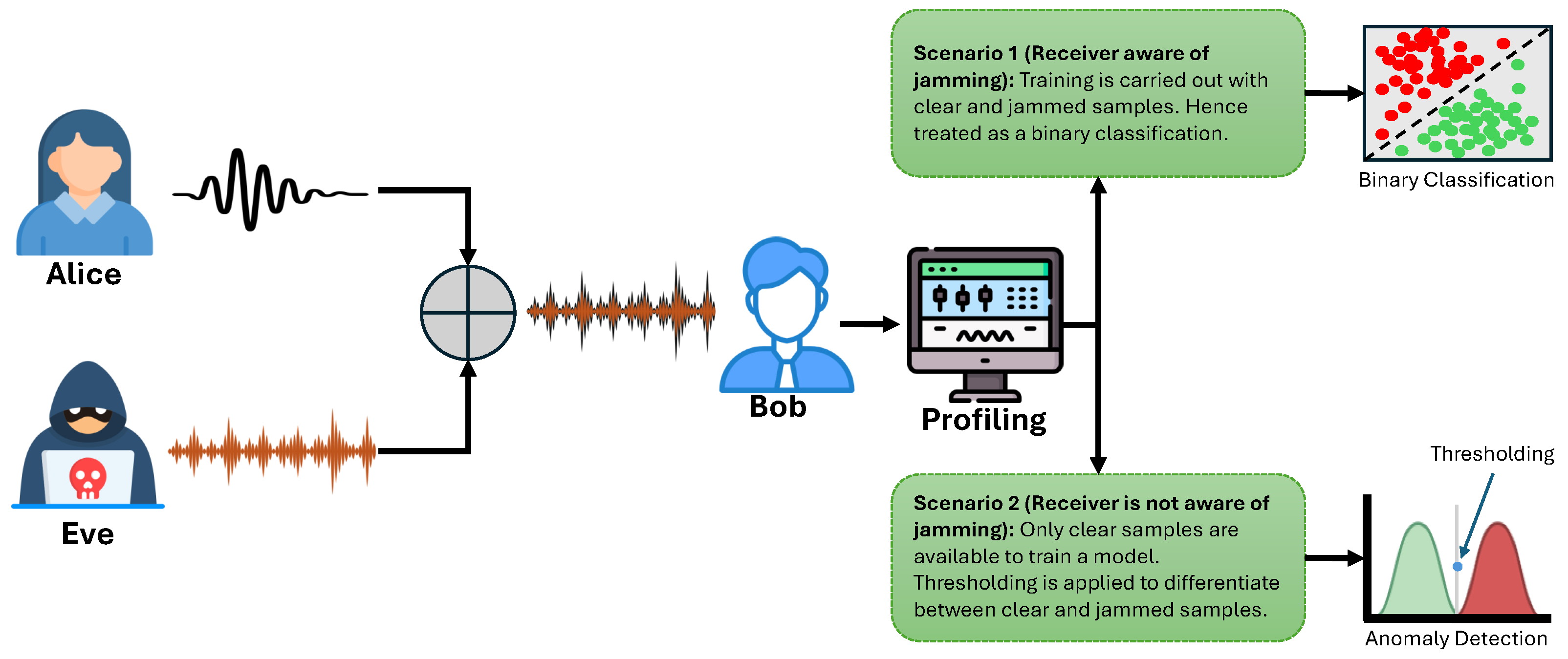
- We consider a brand new scenario that includes “jamming unawareness” during the training of the model, and we compare this scenario with the one previously proposed.
- We improve our system model by formulating the jamming detection as an anomaly detection problem.
- We compare the multi-class classification solution from our previous work with the new one-class classification (based on autoencoders).
- We expand our performance analysis considering multiple parameters, such as channel quality (Signal-to-Noise Ratio (SNR)), training metrics, the level of the Relative Jamming Power (RJP), and the distance of the receiver from the jammer.
2. Related Work

| Paper | Jamming Signal | Technique | Scenario | Signal Representation | Application | Jamming Detection in Regime | Adversary Proximity | Jamming | |
|---|---|---|---|---|---|---|---|---|---|
| Jamming-Pattern-Aware | Jamming-Pattern-Unaware | ||||||||
| Our | AWGN | Spare Autoencoders/CNN | ✓ | ✓ | I−Q Samples | PLC | No-BER | ✓ | ✓ |
| [40] | Sine, Gauss | CNN | ✓ | ✗ | I−Q Samples | Wireless Network | BER | ✓ | ✓ |
| [19] | Sine and Gaussian | Sparse Autoencoder | ✗ | ✓ | I−Q samples | Drone | BER | ✓ | ✓ |
| [35] | AWGN | Gentic CUSUM | ✓ | ✗ | - | Smart Grid | - | ✗ | ✗ |
| [29] | Random | Statistical Process Control | ✓ | ✗ | PDR | Opputnistic Network | Low PDR | ✗ | ✗ |
| [30] | Constant, Reactive, random | Gradient Boosting Algorithm | ✓ | ✗ | PDR and RSS | Ad hoc network | Low PDR | ✓ | ✓ |
| [32] | Constant, Reactive, random | Shallow Neural Network | ✓ | ✗ | PDR | Wireless Network | Low PDR | ✗ | ✓ |
| [33] | Random | Random Forest | ✓ | ✗ | RSSI | Wireless Network | - | - | - |
| [20] | Gaussian | Euclidean Distance | ✓ | ✗ | RSSI and Packet Loss Rate | AMI | Packet Loss Rate | ✗ | ✗ |
| [34] | - | Autoencoder | ✗ | ✓ | Time series data | ICS | - | - | - |
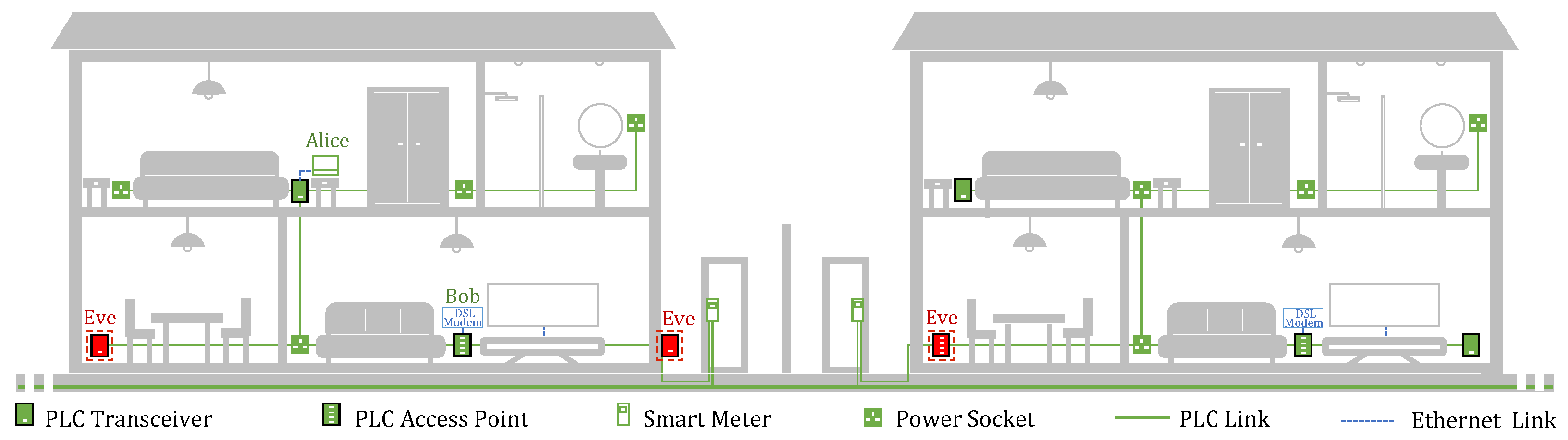
3. Scenario and Adversary Model
4. Background
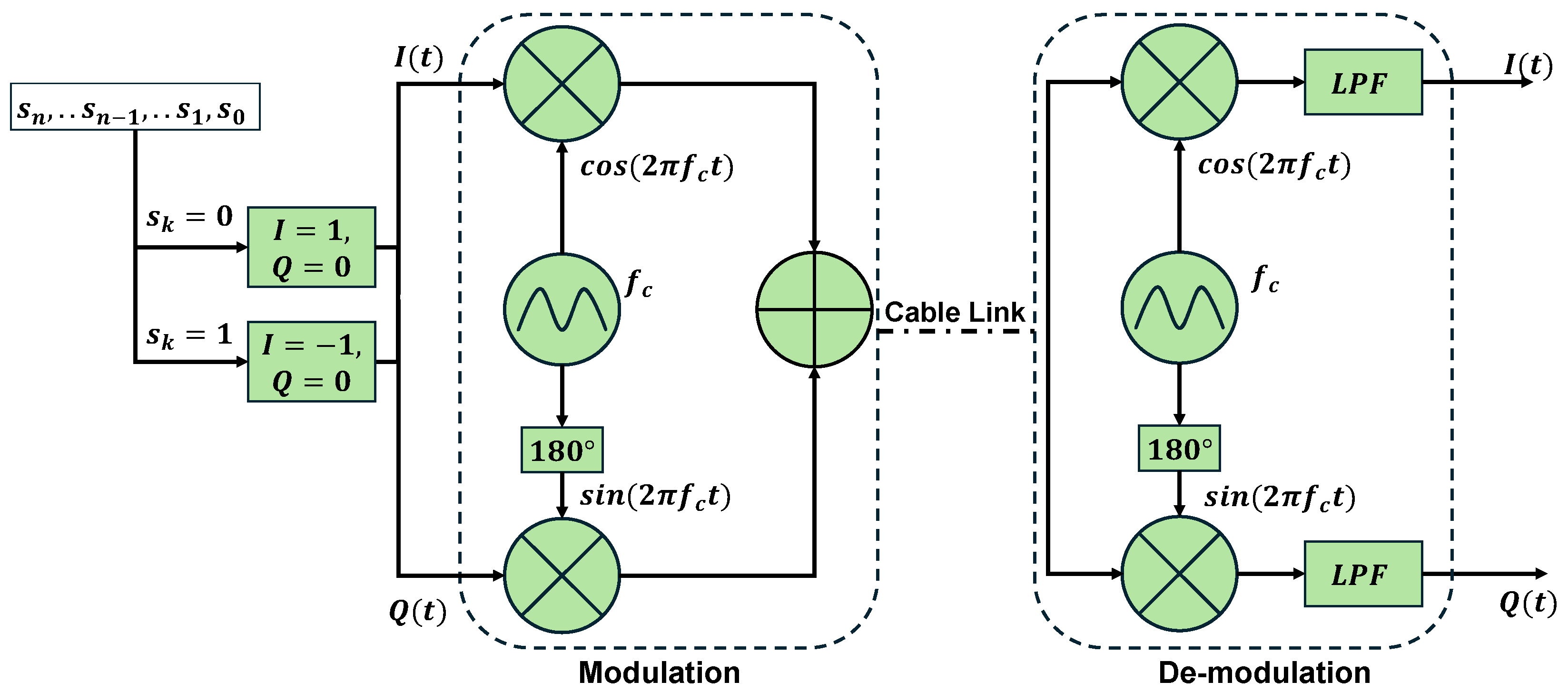
4.1. Digital Modulation
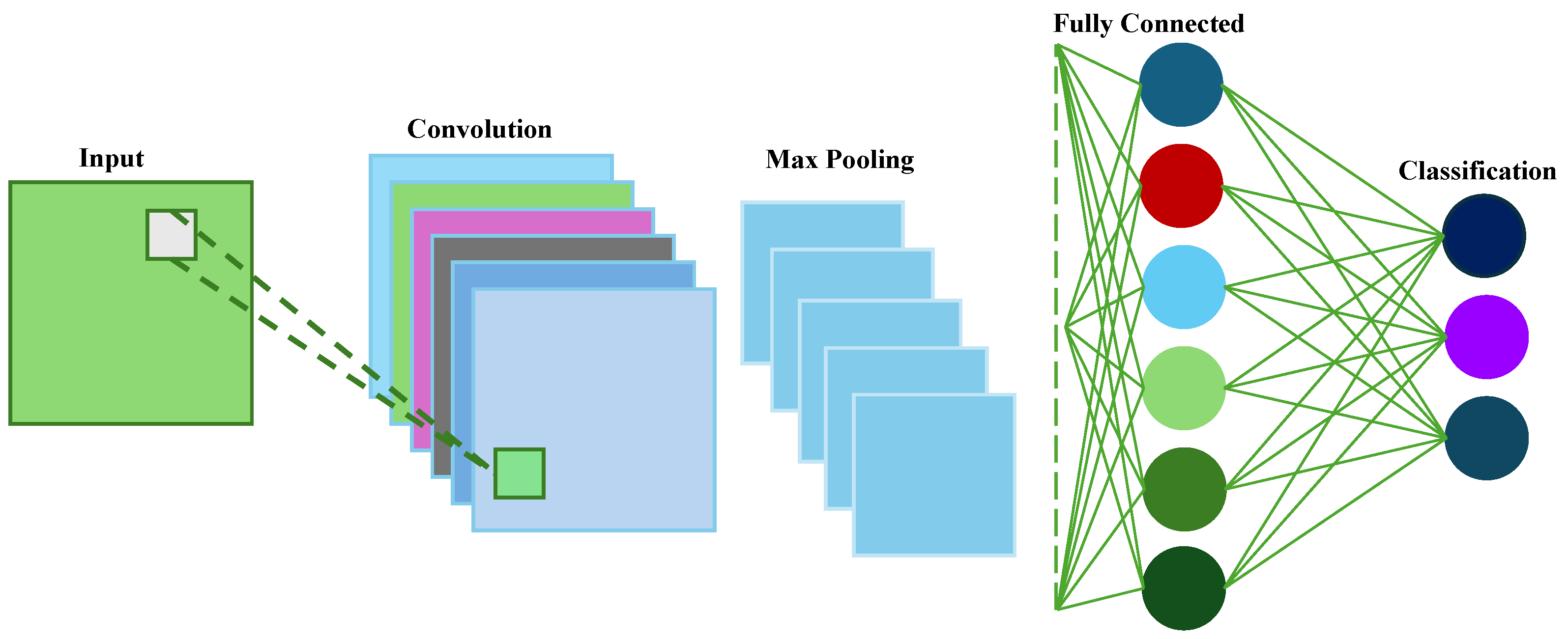
4.2. Convolutional Neural Networks
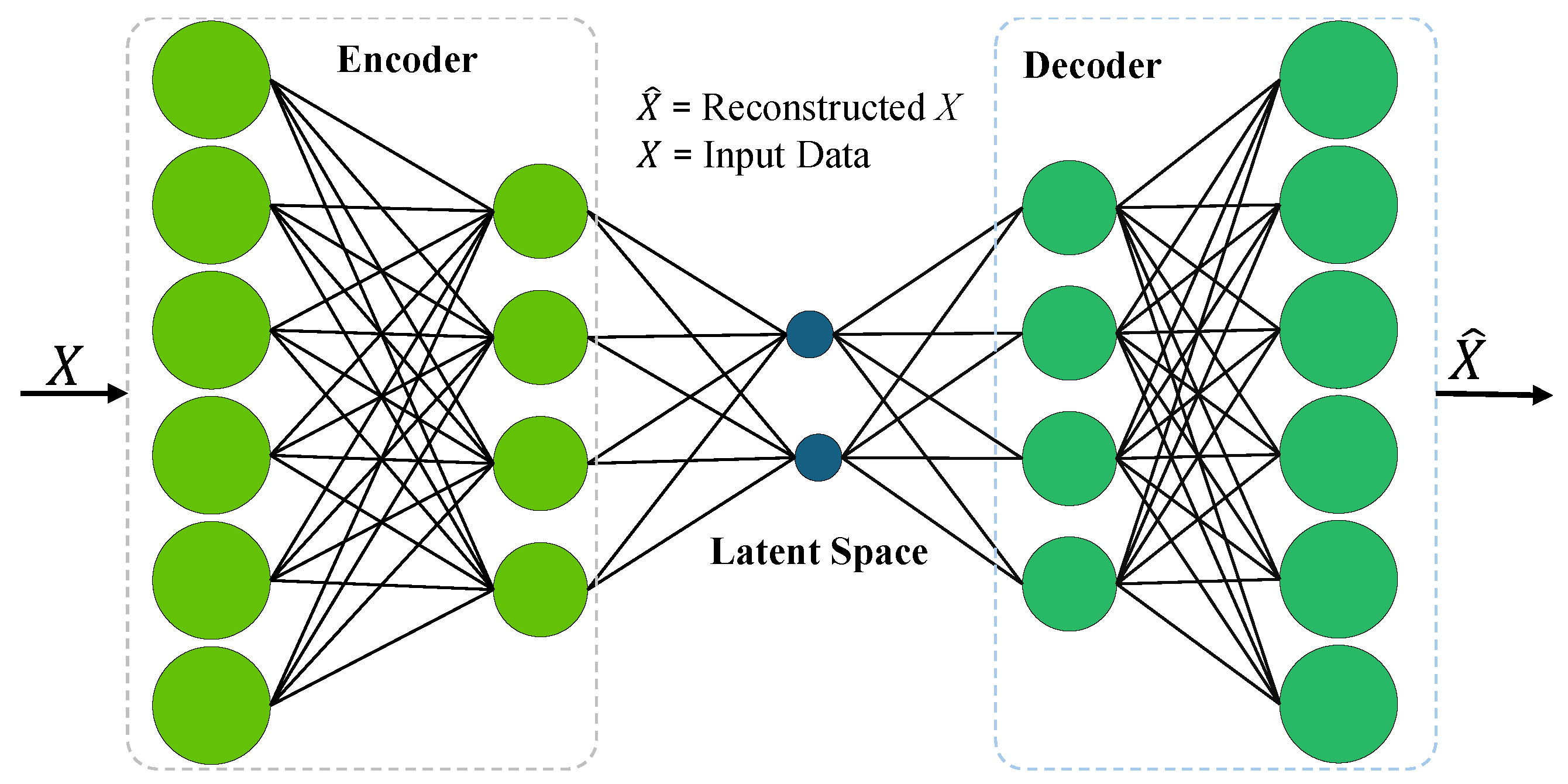
4.3. Autoencoders
5. Theoretical Framework and Methodology
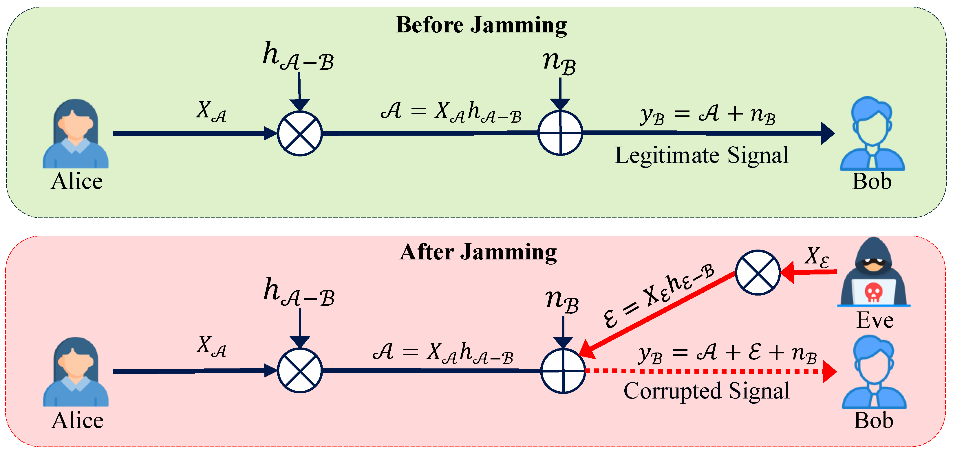
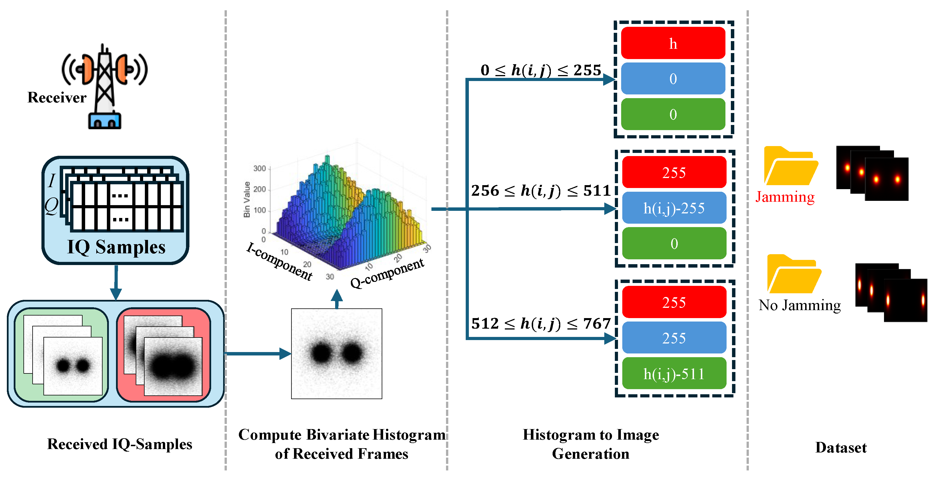
5.1. Theoretical Framework
- For values of such that , the corresponding channel’s pixel values are .
- When the range , pixel values are set according to the following mapping: .
- When , the pixel values are .
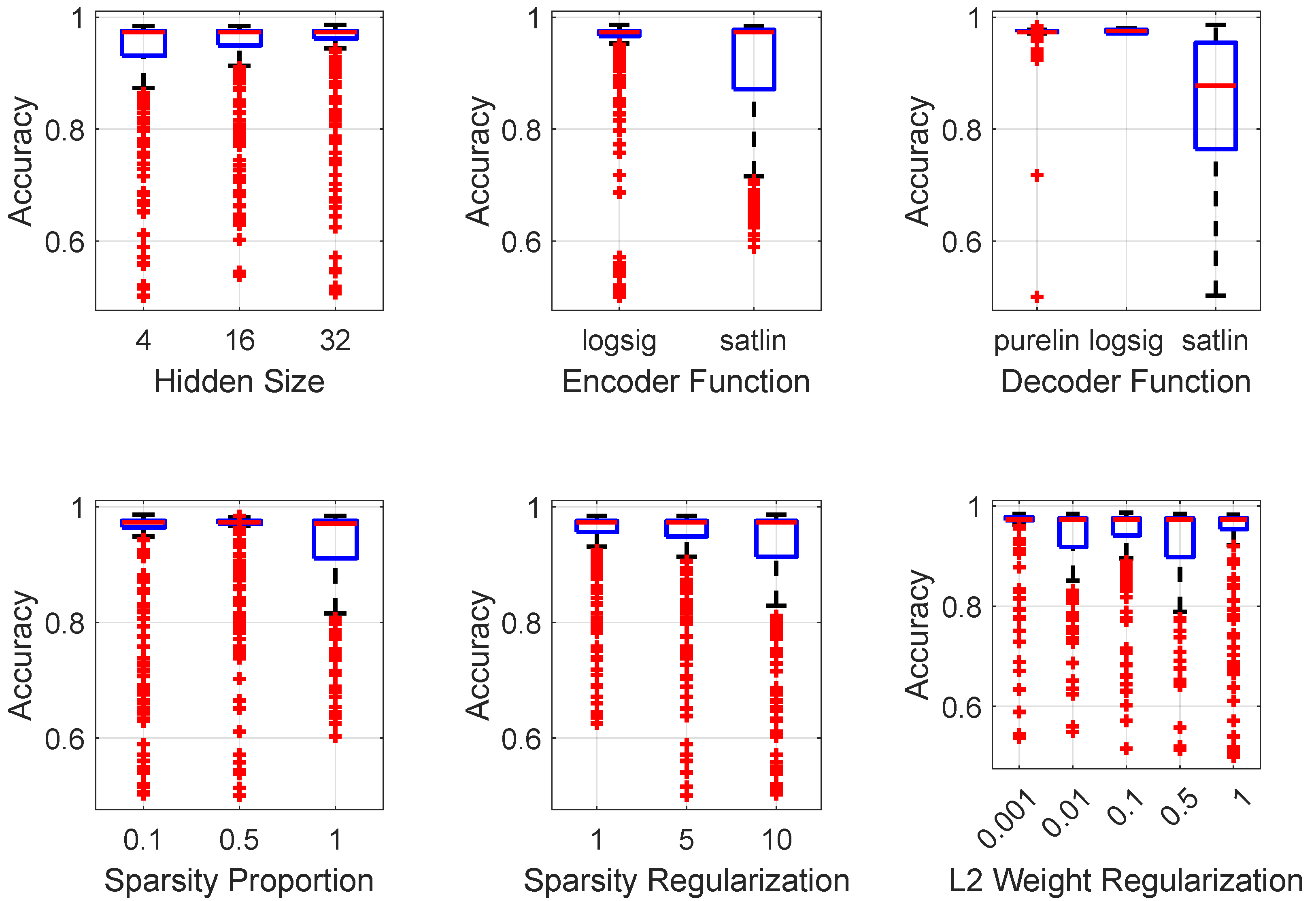
5.2. Hyperparameter Tuning and Statistical Validation
6. Performance Evaluation
6.1. Metrics
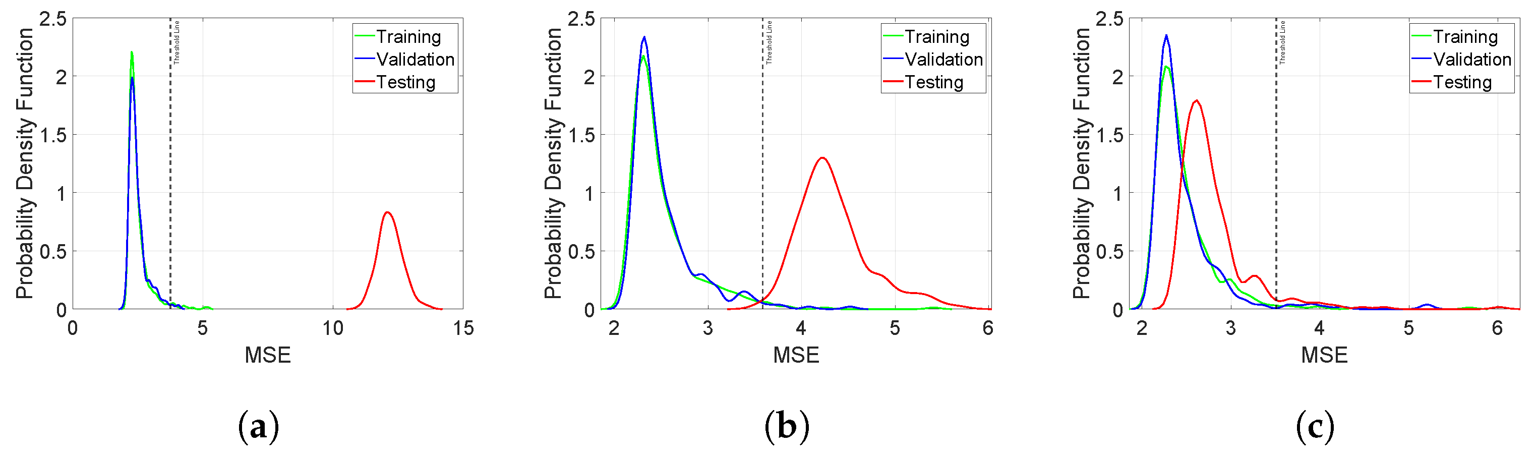
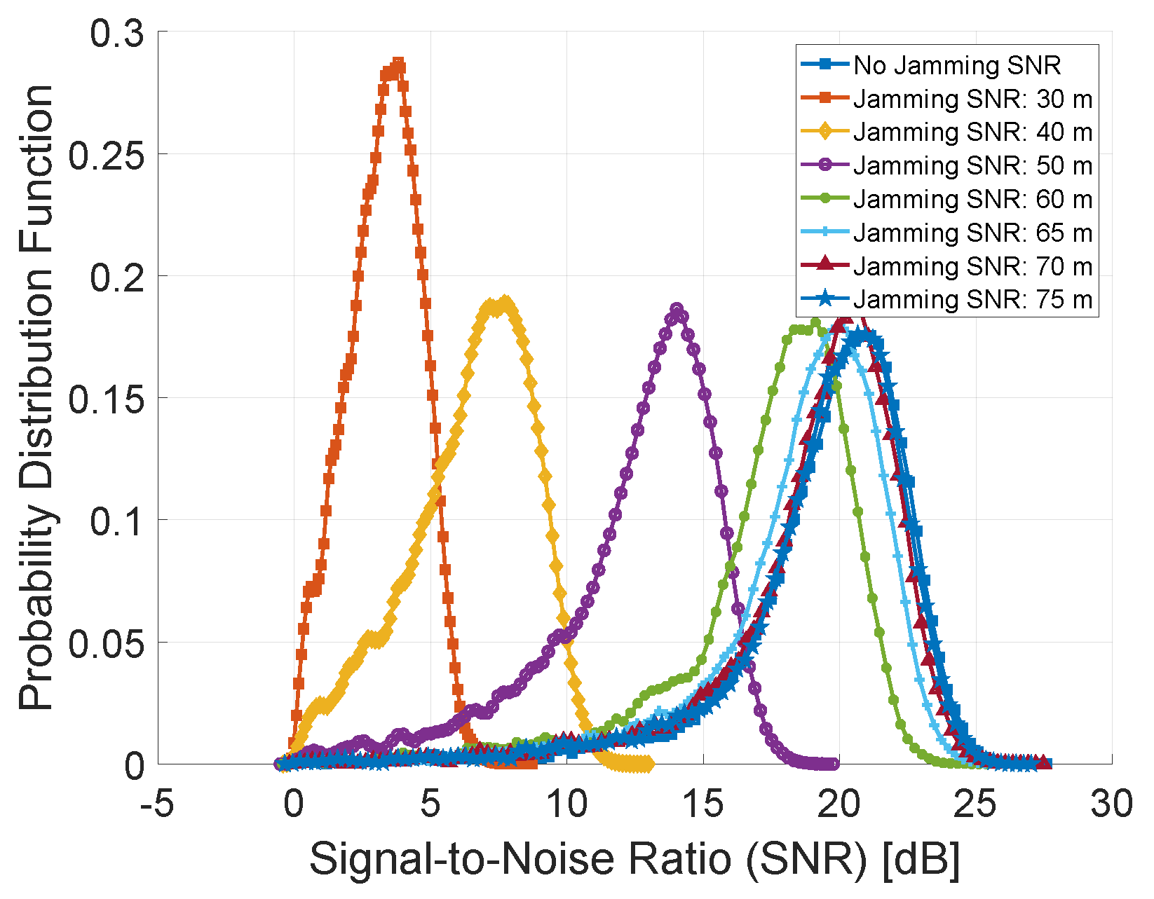
6.2. Link Quality
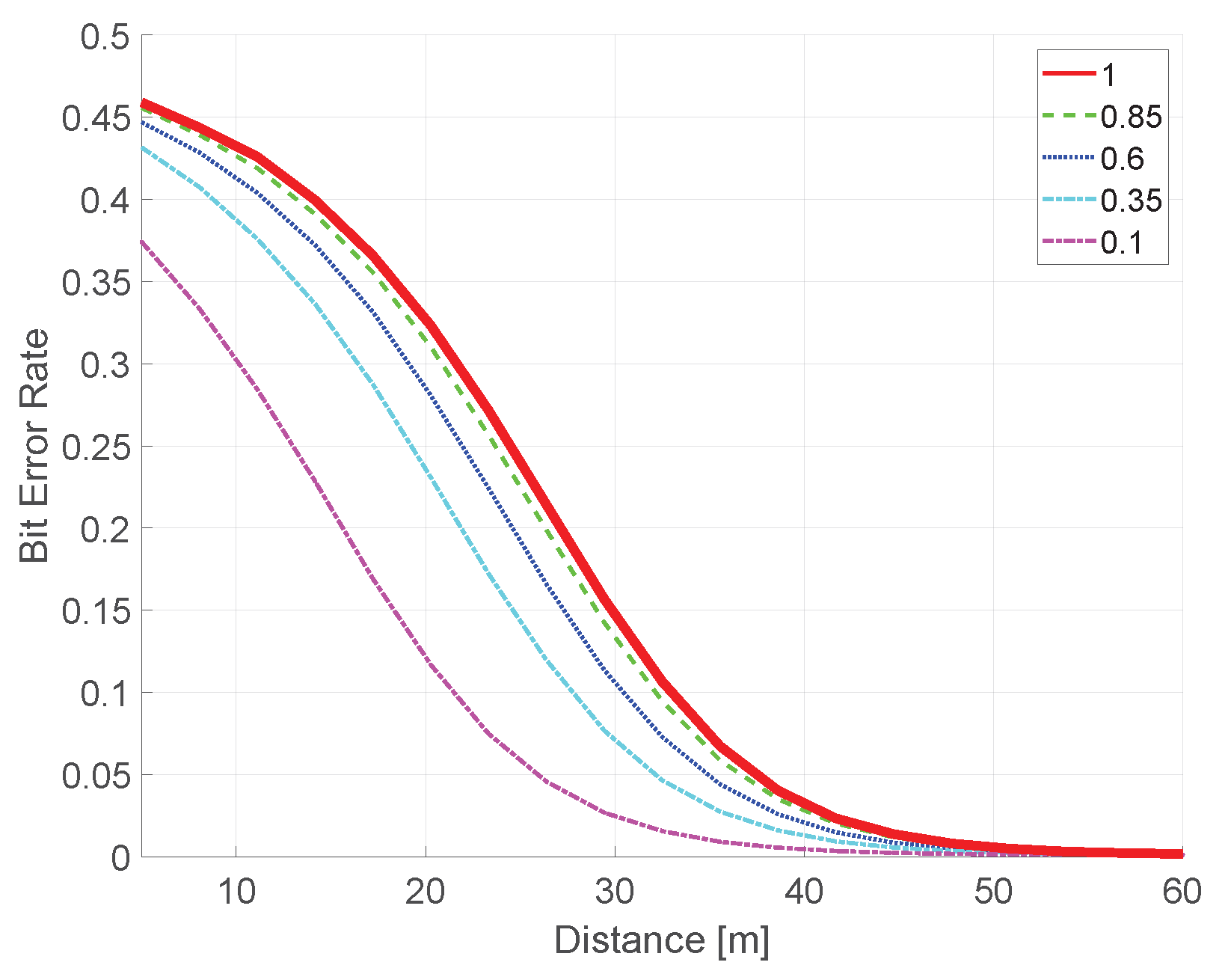
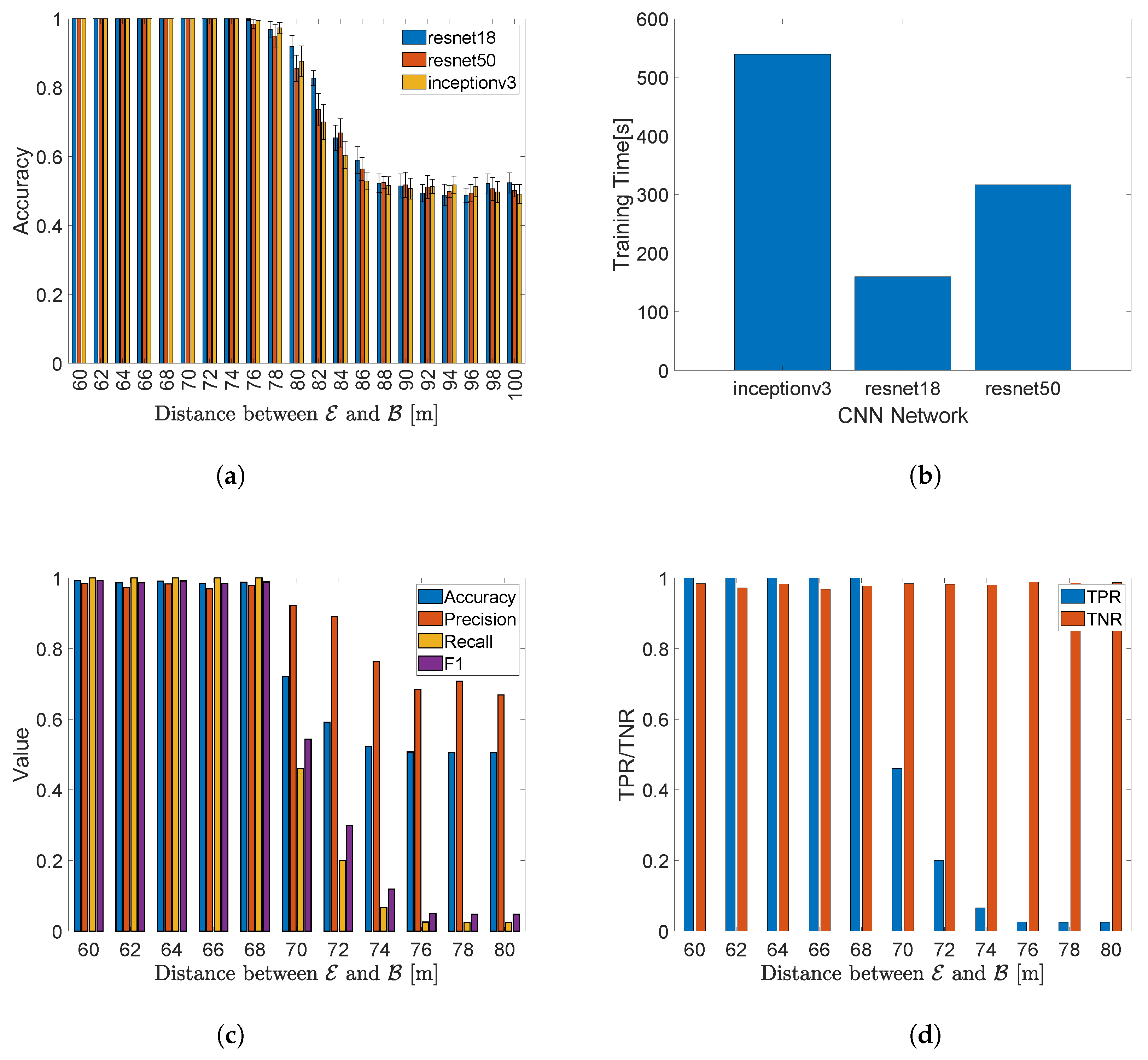
6.3. Distance Between the Jammer and the Receiver
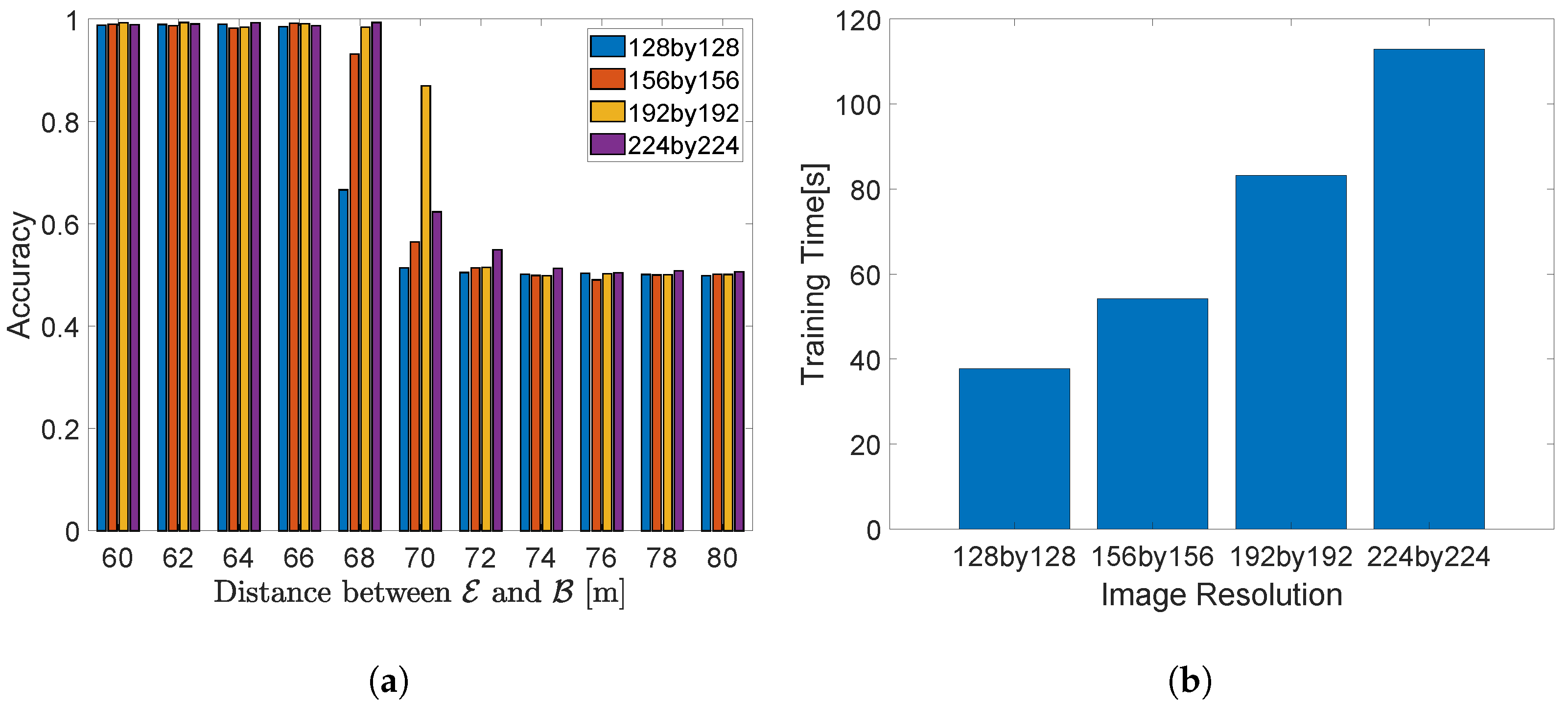
6.4. Image Size
6.5. Relative Jamming Power (RJP)
7. Conclusions
Author Contributions
Funding
Data Availability Statement
Conflicts of Interest
Abbreviations
| AE | Autoencoder |
| AMI | Advanced Metering Infrastructure |
| AWGN | Additive White Gaussian Noise |
| BB-PLC | Broadband PLC |
| BER | Bit Error Rate |
| BPSK | Binary Phase-Shift Keying |
| CNN | Convolutional Neural Network |
| DL | Deep Learning |
| DoS | Denial of Service |
| FN | False Negative |
| FP | False Positive |
| IoT | Internet of Things |
| MSE | Mean Squared Error |
| NB-PLC | Narrowband PLC |
| Probability Density Function | |
| PHY | Physical |
| PLC | Power-Line Communication |
| QPSK | Quadrature Phase-Shift Keying |
| RF | Radio Frequency |
| RJP | Relative Jamming Power |
| SG | Smart Grid |
| SNR | Signal-to-Noise Ratio |
| TNR | True Negative Rate |
| TPR | True Positive Rate |
| UNB-PLC | Ultra-Narrowband PLC |
Appendix A. Different Hyperparameter Search
| En- Coder | Sparsity Prop. | Sparsity Reg. | Weight Reg. | Decoder | |||||||||||
|---|---|---|---|---|---|---|---|---|---|---|---|---|---|---|---|
| logsig | satlin | purelin | |||||||||||||
| Acc | Prec | Rec | F1 | Acc | Prec | Rec | F1 | Acc | Prec | Rec | F1 | ||||
| logsig | 0.10 | 1.00 | 0.001 | 0.99 | 0.97 | 1.00 | 0.99 | 0.80 | 0.95 | 0.63 | 0.76 | 0.98 | 0.97 | 0.99 | 0.98 |
| 0.010 | 0.99 | 0.98 | 1.00 | 0.99 | 0.98 | 0.97 | 0.99 | 0.98 | 0.99 | 0.97 | 1.00 | 0.99 | |||
| 0.100 | 0.98 | 0.96 | 1.00 | 0.98 | 0.92 | 0.99 | 0.84 | 0.91 | 0.99 | 0.98 | 1.00 | 0.99 | |||
| 0.500 | 0.98 | 0.97 | 0.99 | 0.98 | 0.88 | 0.97 | 0.79 | 0.87 | 0.99 | 0.97 | 1.00 | 0.99 | |||
| 1.000 | 0.98 | 0.97 | 1.00 | 0.98 | 0.97 | 0.98 | 0.96 | 0.97 | 0.99 | 0.98 | 1.00 | 0.99 | |||
| 5.00 | 0.001 | 0.99 | 0.98 | 1.00 | 0.99 | 0.85 | 0.98 | 0.72 | 0.83 | 0.98 | 0.96 | 1.00 | 0.98 | ||
| 0.010 | 0.99 | 0.99 | 0.99 | 0.99 | 0.85 | 0.97 | 0.73 | 0.83 | 0.99 | 1.00 | 0.98 | 0.99 | |||
| 0.100 | 0.99 | 0.97 | 1.00 | 0.99 | 0.92 | 0.99 | 0.85 | 0.91 | 0.99 | 0.98 | 1.00 | 0.99 | |||
| 0.500 | 0.99 | 0.98 | 0.99 | 0.99 | 0.95 | 0.99 | 0.92 | 0.95 | 0.99 | 0.99 | 0.99 | 0.99 | |||
| 1.000 | 0.99 | 0.98 | 0.99 | 0.99 | 0.96 | 0.99 | 0.92 | 0.95 | 0.98 | 0.96 | 1.00 | 0.98 | |||
| 0.50 | 1.00 | 0.001 | 0.99 | 0.98 | 1.00 | 0.99 | 0.93 | 0.98 | 0.87 | 0.93 | 0.99 | 0.98 | 1.00 | 0.99 | |
| 0.010 | 0.99 | 0.99 | 0.99 | 0.99 | 0.94 | 0.99 | 0.90 | 0.94 | 0.99 | 0.97 | 1.00 | 0.99 | |||
| 0.100 | 0.99 | 0.99 | 0.99 | 0.99 | 0.93 | 0.97 | 0.89 | 0.93 | 0.99 | 0.98 | 1.00 | 0.99 | |||
| 0.500 | 0.99 | 0.98 | 0.99 | 0.99 | 0.96 | 0.96 | 0.96 | 0.96 | 0.99 | 0.98 | 1.00 | 0.99 | |||
| 1.000 | 0.99 | 0.99 | 0.99 | 0.99 | 0.84 | 1.00 | 0.68 | 0.81 | 0.99 | 0.98 | 1.00 | 0.99 | |||
| 5.00 | 0.001 | 0.99 | 0.98 | 1.00 | 0.99 | 0.98 | 0.98 | 0.99 | 0.98 | 0.99 | 0.98 | 1.00 | 0.99 | ||
| 0.010 | 1.00 | 0.99 | 1.00 | 1.00 | 0.83 | 0.99 | 0.66 | 0.79 | 0.98 | 0.99 | 0.97 | 0.98 | |||
| 0.100 | 0.99 | 0.98 | 1.00 | 0.99 | 0.89 | 0.98 | 0.80 | 0.88 | 0.98 | 0.97 | 1.00 | 0.98 | |||
| 0.500 | 0.98 | 0.96 | 1.00 | 0.98 | 0.86 | 1.00 | 0.73 | 0.84 | 0.99 | 0.98 | 0.99 | 0.99 | |||
| 1.000 | 0.99 | 0.99 | 1.00 | 0.99 | 0.66 | 0.98 | 0.33 | 0.49 | 0.99 | 0.98 | 1.00 | 0.99 | |||
| 1.00 | 1.00 | 0.001 | 1.00 | 0.99 | 1.00 | 1.00 | 0.81 | 0.97 | 0.64 | 0.77 | 0.99 | 0.98 | 0.99 | 0.99 | |
| 0.010 | 0.99 | 0.97 | 1.00 | 0.99 | 0.67 | 0.95 | 0.35 | 0.51 | 0.99 | 0.98 | 1.00 | 0.99 | |||
| 0.100 | 0.99 | 0.98 | 1.00 | 0.99 | 0.58 | 0.94 | 0.17 | 0.29 | 0.99 | 0.97 | 1.00 | 0.99 | |||
| 0.500 | 0.99 | 0.98 | 1.00 | 0.99 | 0.61 | 0.92 | 0.24 | 0.39 | 0.99 | 0.99 | 1.00 | 0.99 | |||
| 1.000 | 0.99 | 0.98 | 1.00 | 0.99 | 0.70 | 0.97 | 0.42 | 0.59 | 1.00 | 0.99 | 1.00 | 1.00 | |||
| 5.00 | 0.001 | 0.99 | 0.99 | 0.99 | 0.99 | 0.82 | 0.99 | 0.64 | 0.78 | 0.99 | 0.97 | 1.00 | 0.99 | ||
| 0.010 | 0.99 | 0.99 | 0.99 | 0.99 | 0.67 | 0.95 | 0.35 | 0.51 | 0.99 | 0.98 | 1.00 | 0.99 | |||
| 0.100 | 0.99 | 0.98 | 1.00 | 0.99 | 0.67 | 0.96 | 0.36 | 0.52 | 0.99 | 0.97 | 1.00 | 0.99 | |||
| 0.500 | 1.00 | 1.00 | 1.00 | 1.00 | 0.69 | 0.98 | 0.40 | 0.56 | 0.98 | 0.97 | 1.00 | 0.98 | |||
| 1.000 | 0.98 | 0.96 | 1.00 | 0.98 | 0.74 | 0.98 | 0.48 | 0.65 | 0.99 | 0.98 | 0.99 | 0.99 | |||
| satlin | 0.10 | 1.00 | 0.001 | 0.98 | 0.96 | 1.00 | 0.98 | 0.56 | 0.81 | 0.15 | 0.26 | 0.99 | 0.99 | 1.00 | 0.99 |
| 0.010 | 0.99 | 0.99 | 1.00 | 0.99 | 0.69 | 0.99 | 0.39 | 0.56 | 0.99 | 0.98 | 1.00 | 0.99 | |||
| 0.100 | 0.99 | 0.98 | 1.00 | 0.99 | 0.63 | 0.96 | 0.27 | 0.43 | 0.99 | 0.98 | 1.00 | 0.99 | |||
| 0.500 | 0.98 | 0.96 | 1.00 | 0.98 | 0.87 | 0.97 | 0.76 | 0.86 | 0.99 | 0.98 | 0.99 | 0.99 | |||
| 1.000 | 0.99 | 0.97 | 1.00 | 0.99 | 0.62 | 0.94 | 0.26 | 0.41 | 0.98 | 0.97 | 1.00 | 0.98 | |||
| 5.00 | 0.001 | 0.99 | 0.98 | 1.00 | 0.99 | 0.59 | 0.96 | 0.18 | 0.31 | 0.99 | 0.98 | 0.99 | 0.99 | ||
| 0.010 | 0.99 | 0.99 | 1.00 | 0.99 | 0.64 | 0.96 | 0.29 | 0.44 | 1.00 | 0.99 | 1.00 | 1.00 | |||
| 0.100 | 0.99 | 0.98 | 0.99 | 0.99 | 0.60 | 0.94 | 0.21 | 0.35 | 0.99 | 0.99 | 0.99 | 0.99 | |||
| 0.500 | 0.99 | 0.98 | 0.99 | 0.99 | 0.66 | 0.97 | 0.32 | 0.49 | 0.99 | 0.99 | 0.99 | 0.99 | |||
| 1.000 | 0.99 | 0.99 | 0.99 | 0.99 | 0.67 | 0.95 | 0.35 | 0.51 | 0.99 | 0.98 | 0.99 | 0.99 | |||
| 0.50 | 1.00 | 0.001 | 0.99 | 0.99 | 1.00 | 0.99 | 0.69 | 0.95 | 0.39 | 0.56 | 0.98 | 0.96 | 1.00 | 0.98 | |
| 0.010 | 0.99 | 0.98 | 0.99 | 0.99 | 0.58 | 0.96 | 0.17 | 0.29 | 0.99 | 0.97 | 1.00 | 0.99 | |||
| 0.100 | 0.99 | 0.99 | 0.99 | 0.99 | 0.69 | 0.98 | 0.39 | 0.56 | 0.99 | 0.99 | 1.00 | 0.99 | |||
| 0.500 | 0.99 | 0.98 | 1.00 | 0.99 | 0.64 | 0.98 | 0.29 | 0.45 | 1.00 | 0.99 | 1.00 | 1.00 | |||
| 1.000 | 0.99 | 0.99 | 0.99 | 0.99 | 0.59 | 0.98 | 0.18 | 0.30 | 0.99 | 0.97 | 1.00 | 0.99 | |||
| 5.00 | 0.001 | 0.99 | 0.99 | 1.00 | 0.99 | 0.54 | 0.82 | 0.09 | 0.17 | 0.99 | 0.99 | 1.00 | 0.99 | ||
| 0.010 | 0.99 | 0.97 | 1.00 | 0.99 | 0.71 | 0.99 | 0.42 | 0.59 | 0.99 | 0.99 | 1.00 | 0.99 | |||
| 0.100 | 0.99 | 0.98 | 0.99 | 0.99 | 0.74 | 0.95 | 0.50 | 0.65 | 0.99 | 0.99 | 1.00 | 0.99 | |||
| 0.500 | 0.99 | 0.99 | 1.00 | 0.99 | 0.63 | 0.95 | 0.28 | 0.43 | 0.99 | 0.98 | 1.00 | 0.99 | |||
| 1.000 | 0.98 | 0.97 | 0.99 | 0.98 | 0.64 | 0.94 | 0.30 | 0.45 | 0.99 | 0.98 | 1.00 | 0.99 | |||
| 1.00 | 1.00 | 0.001 | 0.99 | 0.98 | 1.00 | 0.99 | 0.69 | 0.97 | 0.39 | 0.55 | 0.99 | 0.99 | 1.00 | 0.99 | |
| 0.010 | 0.99 | 0.98 | 1.00 | 0.99 | 0.65 | 0.92 | 0.32 | 0.48 | 0.99 | 0.98 | 1.00 | 0.99 | |||
| 0.100 | 0.98 | 0.96 | 1.00 | 0.98 | 0.70 | 0.95 | 0.42 | 0.58 | 0.99 | 0.98 | 1.00 | 0.99 | |||
| 0.500 | 0.99 | 0.98 | 0.99 | 0.99 | 0.66 | 0.96 | 0.34 | 0.50 | 0.99 | 0.99 | 0.99 | 0.99 | |||
| 1.000 | 0.98 | 0.98 | 0.98 | 0.98 | 0.56 | 0.88 | 0.15 | 0.25 | 0.98 | 0.97 | 1.00 | 0.98 | |||
| 5.00 | 0.001 | 0.99 | 0.99 | 0.99 | 0.99 | 0.70 | 0.95 | 0.42 | 0.59 | 0.99 | 0.98 | 0.99 | 0.99 | ||
| 0.010 | 0.99 | 0.99 | 0.99 | 0.99 | 0.73 | 0.96 | 0.49 | 0.65 | 0.99 | 0.99 | 0.99 | 0.99 | |||
| 0.100 | 0.99 | 0.98 | 0.99 | 0.99 | 0.59 | 0.95 | 0.19 | 0.31 | 0.99 | 0.98 | 1.00 | 0.99 | |||
| 0.500 | 0.99 | 0.98 | 1.00 | 0.99 | 0.77 | 0.97 | 0.56 | 0.71 | 0.98 | 0.97 | 1.00 | 0.98 | |||
| 1.000 | 0.98 | 0.96 | 1.00 | 0.98 | 0.53 | 0.94 | 0.05 | 0.10 | 0.98 | 0.96 | 1.00 | 0.98 | |||
References
- Wadhwani, P. Power Line Communication Market Size, Global Report 2032. Available online: https://www.gminsights.com/industry-analysis/power-line-communication-plc-market (accessed on 6 January 2025).
- Tayade, P. Power Line Communication Market Size and Forecast. Available online: https://www.coherentmarketinsights.com/industry-reports/power-line-communication-market (accessed on 6 January 2025).
- Cano, C.; Pittolo, A.; Malone, D.; Lampe, L.; Tonello, A.M.; Dabak, A.G. State of the art in power line communications: From the applications to the medium. IEEE J. Sel. Areas Commun. 2016, 34, 1935–1952. [Google Scholar] [CrossRef]
- Galli, S.; Scaglione, A.; Wang, Z. For the grid and through the grid: The role of power line communications in the smart grid. Proc. IEEE 2011, 99, 998–1027. [Google Scholar] [CrossRef]
- Raponi, S.; Fernandez, J.H.; Omri, A.; Oligeri, G. Long-Term Noise Characterization of Narrowband Power Line Communications. IEEE Trans. Power Deliv. 2022, 37, 365–373. [Google Scholar] [CrossRef]
- Ghasempour, A. Internet of things in smart grid: Architecture, applications, services, key technologies, and challenges. Inventions 2019, 4, 22. [Google Scholar] [CrossRef]
- Qian, Y.; Shi, L.; Li, J.; Zhou, X.; Shu, F.; Wang, J. An edge-computing paradigm for internet of things over power line communication networks. IEEE Netw. 2020, 34, 262–269. [Google Scholar] [CrossRef]
- Fernandez, J.H.; Omri, A.; Di Pietro, R. Power grid surveillance: Topology change detection system using power line communications. Int. J. Electr. Power Energy Syst. 2023, 145, 108634. [Google Scholar] [CrossRef]
- Omri, A.; Fernandez, J.H.; Di Pietro, R. Extending device noise measurement capacity for OFDM-based PLC systems: Design, implementation, and on-field validation. Comput. Netw. 2023, 237, 110038. [Google Scholar] [CrossRef]
- Fernandez, J.H.; Omri, A.; Oligeri, G. A noise reduction scheme for OFDM NB-PLC systems. E-Prime Electr. Eng. Electron. Energy 2022, 2, 100043. [Google Scholar] [CrossRef]
- Irfan, M.; Omri, A.; Fernandez, J.H.; Sciancalepore, S.; Oligeri, G. Jamming Detection in Power Line Communications Leveraging Deep Learning Techniques. In Proceedings of the International Symposium on Networks, Computers and Communications, Doha, Qatar, 23–26 October 2023; pp. 22–24. [Google Scholar]
- Yin, Z.; Zhang, H.; Liu, W.; Wang, H.; Yin, C. Construction of the Remote Welding System based on Power Line Communication. IOP Conf. Ser. Mater. Sci. Eng. 2019, 612, 042001. [Google Scholar] [CrossRef]
- Ronen, E.; Shamir, A.; Weingarten, A.O.; O’Flynn, C. IoT goes nuclear: Creating a ZigBee chain reaction. In Proceedings of the 2017 IEEE Symposium on Security and Privacy (SP), San Jose, CA, USA, 22–26 May 2017; pp. 195–212. [Google Scholar]
- Yaacoub, J.P.A.; Fernandez, J.H.; Noura, H.N.; Chehab, A. Security of power line communication systems: Issues, limitations and existing solutions. Comput. Sci. Rev. 2021, 39, 100331. [Google Scholar] [CrossRef]
- Fernandez, J.H.; Omri, A.; Di Pietro, R. Performance Analysis of Physical Layer Security in Power Line Communication Networks. In Proceedings of the 2023 IEEE Symposium on Computers and Communications (ISCC), Gammarth, Tunisia, 9–12 July 2023; pp. 777–782. [Google Scholar]
- Camponogara, A.; Poor, H.V.; Ribeiro, M.V. Physical layer security of in-home PLC systems: Analysis based on a measurement campaign. IEEE Syst. J. 2020, 15, 617–628. [Google Scholar] [CrossRef]
- Pittolo, A.; Tonello, A.M. Physical layer security in PLC networks: Achievable secrecy rate and channel effects. In Proceedings of the 2013 IEEE 17th International Symposium on Power Line Communications and Its Applications, Johannesburg, South Africa, 24–27 March 2013; pp. 273–278. [Google Scholar]
- Pittolo, A.; Tonello, A.M. Physical layer security in power line communication networks: An emerging scenario, other than wireless. IET Commun. 2014, 8, 1239–1247. [Google Scholar] [CrossRef]
- Sciancalepore, S.; Kusters, F.; Abdelhadi, N.K.; Oligeri, G. Jamming Detection in Low-BER Mobile Indoor Scenarios via Deep Learning. IEEE Internet Things J. 2023, 11, 14682–14697. [Google Scholar] [CrossRef]
- Asri, S.; Pranggono, B. Impact of distributed denial-of-service attack on advanced metering infrastructure. Wirel. Pers. Commun. 2015, 83, 2211–2223. [Google Scholar] [CrossRef]
- Jin, D.; Nicol, D.M.; Yan, G. An event buffer flooding attack in DNP3 controlled SCADA systems. In Proceedings of the 2011 Winter Simulation Conference (WSC), Phoenix, AZ, USA, 11–14 December 2011; pp. 2614–2626. [Google Scholar]
- Groat, S.; Dunlop, M.; Urbanksi, W.; Marchany, R.; Tront, J. Using an IPv6 moving target defense to protect the Smart Grid. In Proceedings of the 2012 IEEE PES Innovative Smart Grid Technologies (ISGT), Washington, DC, USA, 16–20 January 2012; pp. 1–7. [Google Scholar]
- Zhang, F.; Mahler, M.; Li, Q. Flooding attacks against secure time-critical communications in the power grid. In Proceedings of the 2017 IEEE International Conference on Smart Grid Communications (SmartGridComm), Dresden, Germany, 23–27 October 2017; pp. 449–454. [Google Scholar]
- Chatfield, B.; Haddad, R.J.; Chen, L. Low-computational complexity intrusion detection system for jamming attacks in smart grids. In Proceedings of the 2018 International Conference on Computing, Networking and Communications (ICNC), Maui, HI, USA, 5–8 March 2018; pp. 367–371. [Google Scholar]
- Temple, W.G.; Chen, B.; Tippenhauer, N.O. Delay makes a difference: Smart grid resilience under remote meter disconnect attack. In Proceedings of the 2013 IEEE International Conference on Smart Grid Communications (SmartGridComm), Vancouver, BC, Canada, 21–24 October 2013; pp. 462–467. [Google Scholar]
- Li, H.; Lai, L.; Qiu, R.C. A denial-of-service jamming game for remote state monitoring in smart grid. In Proceedings of the 2011 45th Annual Conference on Information Sciences and Systems, Baltimore, MD, USA, 23–25 March 2011; pp. 1–6. [Google Scholar] [CrossRef]
- Pelechrinis, K.; Iliofotou, M.; Krishnamurthy, S.V. Denial of service attacks in wireless networks: The case of jammers. IEEE Commun. Surv. Tutor. 2010, 13, 245–257. [Google Scholar] [CrossRef]
- Liu, D.; Raymer, J.; Fox, A. Efficient and timely jamming detection in wireless sensor networks. In Proceedings of the 2012 IEEE 9th International Conference on Mobile Ad-Hoc and Sensor Systems (MASS 2012), Las Vegas, NV, USA, 8–11 October 2012; pp. 335–343. [Google Scholar] [CrossRef]
- Singh, J.; Woungang, I.; Dhurandher, S.K.; Khalid, K. A jamming attack detection technique for opportunistic networks. Internet Things 2022, 17, 100464. [Google Scholar] [CrossRef]
- Kasturi, G.; Jain, A.; Singh, J. Detection and Classification of Radio Frequency Jamming Attacks using Machine learning. J. Wirel. Mob. Netw. Ubiquitous Comput. Dependable Appl. 2020, 11, 49–62. [Google Scholar]
- Manesh, M.R.; Velashani, M.S.; Ghribi, E.; Kaabouch, N. Performance comparison of machine learning algorithms in detecting jamming attacks on ADS-B devices. In Proceedings of the 2019 IEEE International Conference on Electro Information Technology (EIT), Brookings, SD, USA, 20–22 May 2019; pp. 200–206. [Google Scholar]
- Testi, E.; Arcangeloni, L.; Giorgetti, A. Machine learning-based jamming detection and classification in wireless networks. In Proceedings of the 2023 ACM Workshop on Wireless Security and Machine Learning, Guildford, UK, 1 June 2023; pp. 39–44. [Google Scholar]
- Upadhyaya, B.; Sun, S.; Sikdar, B. Machine learning-based jamming detection in wireless IoT networks. In Proceedings of the 2019 IEEE VTS Asia Pacific Wireless Communications Symposium (APWCS), Singapore, 28–30 August 2019; pp. 1–5. [Google Scholar]
- Wang, C.; Wang, B.; Liu, H.; Qu, H. Anomaly detection for industrial control system based on autoencoder neural network. Wirel. Commun. Mob. Comput. 2020, 2020, 8897926. [Google Scholar] [CrossRef]
- Lu, K.D.; Wu, Z.G. Genetic algorithm-based cumulative sum method for jamming attack detection of cyber-physical power systems. IEEE Trans. Instrum. Meas. 2022, 71, 1–10. [Google Scholar] [CrossRef]
- Soltanieh, N.; Norouzi, Y.; Yang, Y.; Karmakar, N.C. A review of radio frequency fingerprinting techniques. IEEE J. Radio Freq. Identif. 2020, 4, 222–233. [Google Scholar] [CrossRef]
- Abbas, S.; Abu Talib, M.; Nasir, Q.; Idhis, S.; Alaboudi, M.; Mohamed, A. Radio frequency fingerprinting techniques for device identification: A survey. Int. J. Inf. Secur. 2024, 23, 1389–1427. [Google Scholar] [CrossRef]
- Ross, B.P.; Carbino, T.J.; Stone, S.J. Physical-layer discrimination of power line communications. In Proceedings of the 2017 International Conference on Computing, Networking and Communications (ICNC), Silicon Valley, CA, USA, 26–29 January 2017; pp. 341–345. [Google Scholar]
- Carbino, T.J.; Temple, M.A.; Lopez, J. Conditional Constellation Based-Distinct Native Attribute (CB-DNA) fingerprinting for network device authentication. In Proceedings of the 2016 IEEE International Conference on Communications (ICC), Kuala Lumpur, Malaysia, 22–27 May 2016; pp. 1–6. [Google Scholar] [CrossRef]
- Alhazbi, S.; Sciancalepore, S.; Oligeri, G. BloodHound: Early Detection and Identification of Jamming at the PHY-layer. In Proceedings of the 2023 IEEE 20th Consumer Communications & Networking Conference (CCNC), Las Vegas, NV, USA, 8–11 January 2023; pp. 1033–1041. [Google Scholar]
- Rappaport, T.S. Wireless Communications–Principles and Practice, (The Book End). Microw. J. 2002, 45, 128–129. [Google Scholar]
- Large, D.; Farmer, J. Modern Cable Television Technology; Elsevier: Amsterdam, The Netherlands, 2004. [Google Scholar]
- Meng, H.; Guan, Y.L.; Chen, S. Modeling and analysis of noise effects on broadband power-line communications. IEEE Trans. Power Deliv. 2005, 20, 630–637. [Google Scholar] [CrossRef]
- Microchip. Consumer-Band Bpsk 7.2 Kbps Power-Line Soft-Modem Pictail Plus Daughter Board. 2024. Available online: https://www.microchip.com/en-us/development-tool/ac164142 (accessed on 14 May 2025).
- Galvez, R.L.; Bandala, A.A.; Dadios, E.P.; Vicerra, R.R.P.; Maningo, J.M.Z. Object detection using convolutional neural networks. In Proceedings of the TENCON 2018-2018 IEEE Region 10 Conference, Jeju, Reublic of Korea, 28–31 October 2018; pp. 2023–2027. [Google Scholar]
- Tien, P.W.; Wei, S.; Liu, T.; Calautit, J.; Darkwa, J.; Wood, C. A deep learning approach towards the detection and recognition of opening of windows for effective management of building ventilation heat losses and reducing space heating demand. Renew. Energy 2021, 177, 603–625. [Google Scholar] [CrossRef]
- Islam, M.Z.; Islam, M.M.; Asraf, A. A combined deep CNN-LSTM network for the detection of novel coronavirus (COVID-19) using X-ray images. Inform. Med. Unlocked 2020, 20, 100412. [Google Scholar] [CrossRef]
- Kleesiek, J.; Urban, G.; Hubert, A.; Schwarz, D.; Maier-Hein, K.; Bendszus, M.; Biller, A. Deep MRI brain extraction: A 3D convolutional neural network for skull stripping. NeuroImage 2016, 129, 460–469. [Google Scholar] [CrossRef]
- Ge, S.; Li, J.; Ye, Q.; Luo, Z. Detecting masked faces in the wild with lle-cnns. In Proceedings of the IEEE Conference on Computer Vision and Pattern Recognition, Honolulu, HI, USA, 21–26 July 2017; pp. 2682–2690. [Google Scholar]
- Li, H.; Lin, Z.; Shen, X.; Brandt, J.; Hua, G. A convolutional neural network cascade for face detection. In Proceedings of the IEEE Conference on Computer Vision and Pattern Recognition, Boston, MA, USA, 7–12 June 2015; pp. 5325–5334. [Google Scholar]
- Duan, Y.; Lu, J.; Zhou, J. Uniformface: Learning deep equidistributed representation for face recognition. In Proceedings of the IEEE/CVF Conference on Computer Vision and Pattern Recognition, Long Beach, CA, USA, 15–20 June 2019; pp. 3415–3424. [Google Scholar]
- Liu, X.; Kumar, B.; Yang, C.; Tang, Q.; You, J. Dependency-aware attention control for unconstrained face recognition with image sets. In Proceedings of the European Conference on Computer Vision (ECCV), Munich, Germany, 8–14 September 2018; pp. 548–565. [Google Scholar]
- Nair, V.; Hinton, G.E. Rectified linear units improve restricted boltzmann machines. In Proceedings of the 27th International Conference on Machine Learning (ICML-10), Haifa, Israel, 21–24 June 2010; pp. 807–814. [Google Scholar]
- LeCun, Y.; Bottou, L.; Orr, G.B.; Müller, K.R. Efficient backprop. In Neural Networks: Tricks of the Trade; Springer: Berlin/Heidelberg, Germany, 2002; pp. 9–50. [Google Scholar]
- Bank, D.; Koenigstein, N.; Giryes, R. Machine learning for data science handbook: Data mining and knowledge discovery handbook. Autoencoders 2023, 353–374. [Google Scholar]
- Oligeri, G.; Sciancalepore, S.; Raponi, S.; Di Pietro, R. PAST-AI: Physical-layer authentication of satellite transmitters via deep learning. IEEE Trans. Inf. Forensics Secur. 2022, 18, 274–289. [Google Scholar] [CrossRef]
- Michelucci, U. An introduction to autoencoders. arXiv 2022, arXiv:2201.03898. [Google Scholar]
- Mathur, A.; Bhatnagar, M.R.; Panigrahi, B.K. PLC Performance Analysis Over Rayleigh Fading Channel Under Nakagami-m Additive Noise. IEEE Commun. Lett. 2014, 18, 2101–2104. [Google Scholar] [CrossRef]
- Abou-Rjeily, C. Power Line Communications Under Rayleigh Fading and Nakagami Noise: Novel Insights on the MIMO and Multi-Hop Techniques. IET Commun. 2018, 12, 184–191. [Google Scholar] [CrossRef]
- Ai, Y.; Cheffena, M. Capacity Analysis of PLC over Rayleigh Fading Channels with Colored Nakagami-m Additive Noise. In Proceedings of the 2016 IEEE 84th Vehicular Technology Conference (VTC-Fall), Montreal, QC, Canada, 18–21 September 2016; pp. 1–5. [Google Scholar]
- Alhazbi, S.; Sciancalepore, S.; Oligeri, G. The day-after-tomorrow: On the performance of radio fingerprinting over time. In Proceedings of the 39th Annual Computer Security Applications Conference, Austin, TX, USA, 4–8 December 2023; pp. 439–450. [Google Scholar]
- Russakovsky, O.; Deng, J.; Su, H.; Krause, J.; Satheesh, S.; Ma, S.; Huang, Z.; Karpathy, A.; Khosla, A.; Bernstein, M.; et al. ImageNet Large Scale Visual Recognition Challenge. Int. J. Comp. Vis. 2015, 115, 211–252. [Google Scholar] [CrossRef]
- Erfani, S.M.; Rajasegarar, S.; Karunasekera, S.; Leckie, C. High-dimensional and large-scale anomaly detection using a linear one-class SVM with deep learning. Pattern Recognit. 2016, 58, 121–134. [Google Scholar] [CrossRef]
- Qu, Q.; Wei, S.; Liu, S.; Liang, J.; Shi, J. JRNet: Jamming recognition networks for radar compound suppression jamming signals. IEEE Trans. Veh. Technol. 2020, 69, 15035–15045. [Google Scholar] [CrossRef]
- Cai, Y.; Shi, K.; Song, F.; Xu, Y.; Wang, X.; Luan, H. Jamming pattern recognition using spectrum waterfall: A deep learning method. In Proceedings of the 2019 IEEE 5th International Conference on Computer and Communications (ICCC), Chengdu, China, 6–9 December 2019; pp. 2113–2117. [Google Scholar]
- Olshausen, B.; Field, D. Sparse coding with an overcomplete basis set: A strategy employed by V1? Vis. Res. 1997, 37, 3311–3325. [Google Scholar] [CrossRef]


| Parameter | Notation | Value |
|---|---|---|
| Transmit Power [dBV] | 120 | |
| Noise Power [dBV] | 70 | |
| Number of SC per OFDM Symbol | 512 | |
| FFT Size | 512 | |
| Carrier Frequency [Hz] | 20 × | |
| Sub-Carrier Spacing [Hz] | 15 × | |
| OFDM Symbols per Frame | 20 | |
| Sampling Time [s] | ||
| OFDM Symbol Duration [s] | ||
| Frame Duration [s] | ||
| Number of Frames | ||
| Number of OFDM Symbols | ||
| Distance – [m] | 30 | |
| Distance – [m] | ≥60 | |
| Simulation time [s] | 2 |
| Image Resolution | No. of Samples | No Jamming [Images] | Jamming [Images] |
|---|---|---|---|
| 655,360 | 750 | 750 | |
| 471,040 | 750 | 750 | |
| 317,440 | 750 | 750 | |
| 204,800 | 750 | 750 |
| Hyperparameter | Search Range | Optimal Configuration |
|---|---|---|
| Hidden Layer Size | {4, 16, 32} | 32 |
| Encoder Transfer Function | {logsig, satlin} | logsig |
| Decoder Transfer Function | {logsig, satlin, purelin} | satlin |
| Sparsity Proportion | {0.1, 0.5, 1.0} | 0.1 |
| Sparsity Regularization | {1, 5, 10} | 10.0 |
| Weight Regularization | {0.001, 0.01, 0.1, 0.5, 1.0} | 0.1 |
| Training Epochs | 50 | 50 |
Disclaimer/Publisher’s Note: The statements, opinions and data contained in all publications are solely those of the individual author(s) and contributor(s) and not of MDPI and/or the editor(s). MDPI and/or the editor(s) disclaim responsibility for any injury to people or property resulting from any ideas, methods, instructions or products referred to in the content. |
© 2025 by the authors. Licensee MDPI, Basel, Switzerland. This article is an open access article distributed under the terms and conditions of the Creative Commons Attribution (CC BY) license (https://creativecommons.org/licenses/by/4.0/).
Share and Cite
Irfan, M.; Omri, A.; Hernandez Fernandez, J.; Sciancalepore, S.; Oligeri, G. Detecting Jamming in Smart Grid Communications via Deep Learning. J. Cybersecur. Priv. 2025, 5, 46. https://doi.org/10.3390/jcp5030046
Irfan M, Omri A, Hernandez Fernandez J, Sciancalepore S, Oligeri G. Detecting Jamming in Smart Grid Communications via Deep Learning. Journal of Cybersecurity and Privacy. 2025; 5(3):46. https://doi.org/10.3390/jcp5030046
Chicago/Turabian StyleIrfan, Muhammad, Aymen Omri, Javier Hernandez Fernandez, Savio Sciancalepore, and Gabriele Oligeri. 2025. "Detecting Jamming in Smart Grid Communications via Deep Learning" Journal of Cybersecurity and Privacy 5, no. 3: 46. https://doi.org/10.3390/jcp5030046
APA StyleIrfan, M., Omri, A., Hernandez Fernandez, J., Sciancalepore, S., & Oligeri, G. (2025). Detecting Jamming in Smart Grid Communications via Deep Learning. Journal of Cybersecurity and Privacy, 5(3), 46. https://doi.org/10.3390/jcp5030046