Generative Modeling for Imbalanced Credit Card Fraud Transaction Detection

Abstract

The increasing sophistication of fraud tactics necessitates advanced detection methods to protect financial assets and maintain system integrity. Various approaches based on artificial intelligence have been proposed to identify fraudulent activities, leveraging techniques such as machine learning and deep learning. However, class imbalance remains a significant challenge. We propose several solutions based on advanced generative modeling techniques to address the challenges posed by class imbalance in fraud detection. Class imbalance often hinders the performance of machine learning models by limiting their ability to learn from minority classes, such as fraudulent transactions. Generative models offer a promising approach to mitigate this issue by creating realistic synthetic samples, thereby enhancing the model’s ability to detect rare fraudulent cases. In this study, we introduce and evaluate multiple generative models, including Variational Autoencoders (VAEs), standard Autoencoders (AEs), Generative Adversarial Networks (GANs), and a hybrid Autoencoder–GAN model (AE-GAN). These models aim to generate synthetic fraudulent samples to balance the dataset and improve the model’s learning capacity. Our primary objective is to compare the performance of these generative models against traditional oversampling techniques, such as SMOTE and ADASYN, in the context of fraud detection. We conducted extensive experiments using a real-world credit card dataset to evaluate the effectiveness of our proposed solutions. The results, measured using the BEFS metrics, demonstrate that our generative models not only address the class imbalance problem more effectively but also outperform conventional oversampling methods in identifying fraudulent transactions.

1. Introduction

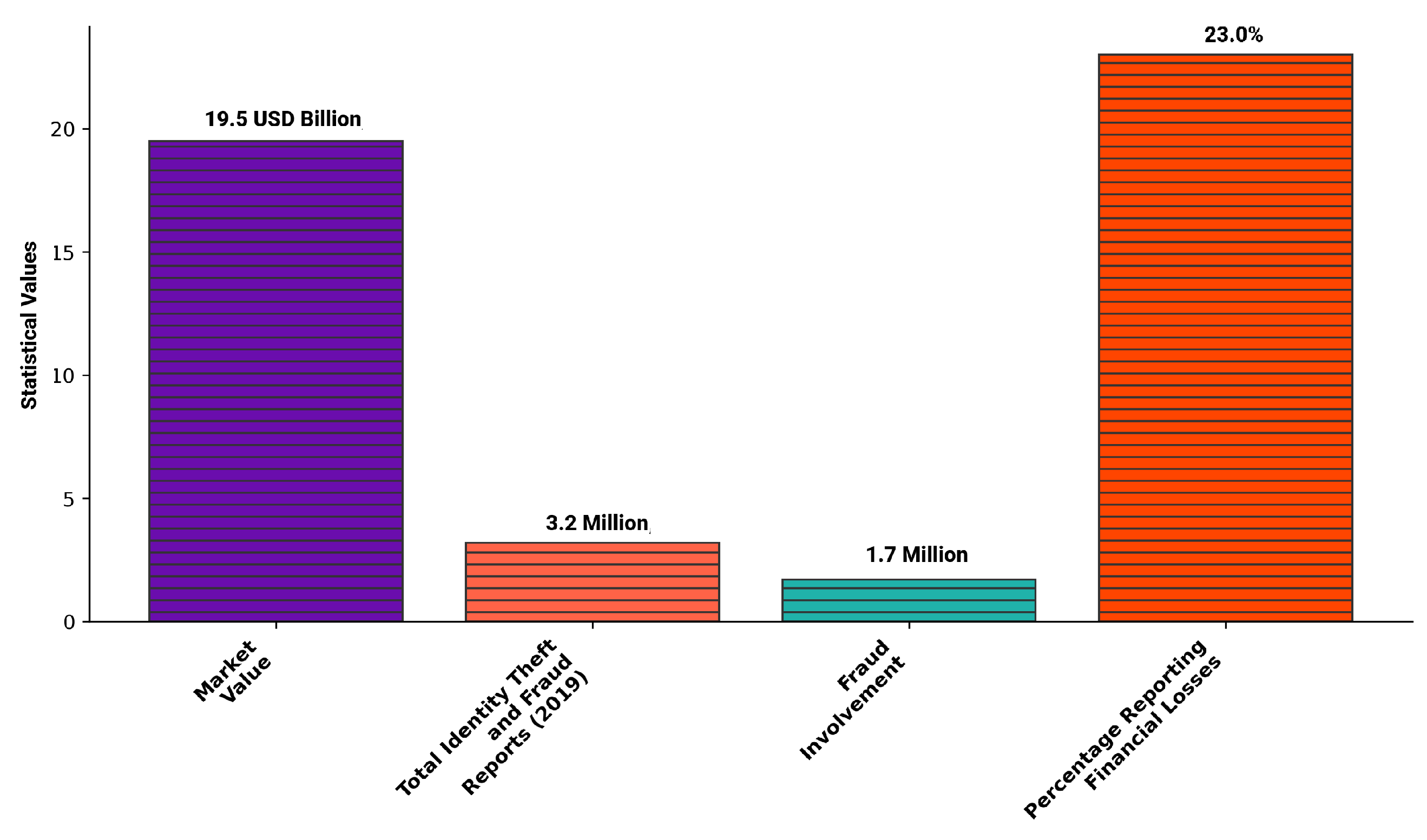
Recent studies estimate that the fraud detection and prevention market is valued at USD 19.5 billion. According to the Consumer Sentinel Network in the USA, among the 3.2 million identity theft and fraud reports in 2019, 1.7 million involved fraud [1]. Of these cases, 23% reported financial losses, highlighting the significant impact on both institutions and individuals. Rapid detection of fraudulent activities is crucial and should occur as soon as streams containing relevant financial data are received. This urgency results in extensive datasets within financial institutions, which are often complex due to the diverse features recorded in transactions [2]. Figure 1 shows the statistical number discussed above in a better manner.

Financial institutions are tasked with the critical challenge of quickly and accurately identifying and isolating fraudulent transactions while maintaining a smooth customer experience. “Quickly” emphasizes the need for a detection model that minimizes delays, protecting both customers and institutions from potential issues. Meanwhile, “accurately” highlights the importance of precise fraud detection, as false positives can lead to unnecessary resource allocation [3]. Traditionally, fraud detection methods, such as manual review or rule-based models, have shown limited effectiveness. Manual detection is slow, requiring a long time to conclude, while rule-based approaches involve complex rules that must be applied and assessed before a transaction can be labeled as suspicious [4]. Both methods demand significant effort to establish criteria for identifying fraudulent transactions and struggle to detect new, unknown, and sophisticated fraud patterns. For this reason, financial institutions spend a lot of money searching for powerful techniques to prevent fraudulent transactions with higher accuracy by employing artificial intelligence. AI-driven fraud detection systems provide unmatched speed, efficiency, and adaptability [5]. Machine learning models (ML), such as Logistic Regression, Decision Tree, Random Forest, Gradient Boosting, XGBoost, LightGBM, K-Nearest Neighbors, Naive Bayes, AdaBoost, and Bagging Classifier, offer a range of solutions for detecting fraudulent transactions [6]. These models are effective at handling various data patterns and can be used individually or combined to enhance fraud detection capabilities [7]. Likewise, deep learning techniques (DL), including Long Short-Term Memory networks, Artificial Neural Networks, and Recurrent Neural Networks, further strengthen these solutions by analyzing large datasets and uncovering intricate patterns [8]. The integration of these ML and DL models into hybrid algorithms provides a comprehensive approach to fraud detection. Hybrid models leverage diverse techniques to improve detection accuracy, reduce false positives, and adapt to evolving fraud tactics [9]. They also optimize computational resources for scalability, ensuring efficient performance even with large-scale data. As financial fraud becomes increasingly sophisticated, the application of advanced ML and DL models helps institutions stay ahead of threats, manage risks effectively, comply with regulations, and protect against financial losses [10].

Class imbalance is a critical challenge in machine learning problems because it poses significant issues for most machine learning algorithms. By default, these algorithms optimize overall accuracy, which can cause models to ignore the minority class, prioritizing correct predictions for the majority while failing to detect rare but critical instances. For example, in fraud detection, fraudulent transactions may represent less than 1% of all data, allowing a model to achieve 99% accuracy by naively labeling every transaction as legitimate [11]. However, accurately identifying rare fraudulent transactions is critical for financial institutions to prevent losses. The imbalance makes it difficult for classifiers to effectively learn from the limited examples of fraudulent transactions [12]. Traditional methods designed for balanced datasets often focus on overall accuracy, which can result in poor performance in detecting the minority class. To tackle this issue, several techniques have been developed [13]. Data-level methods, such as oversampling and undersampling, aim to adjust the dataset to mitigate the imbalance. Oversampling increases the number of fraudulent transaction samples by duplicating them, while undersampling reduces the number of legitimate transactions, potentially at the cost of losing valuable information [4]. Advanced methods like the Synthetic Minority Oversampling Technique (SMOTE) generate synthetic examples of fraudulent transactions [14], and its variants—like the Adaptive Synthetic Sampling Approach (ADASYN) [15], Borderline-SMOTE, Majority Weighted Minority Oversampling Technique (MWMOTE), and Weighted Kernel-Based SMOTE—generate synthetic samples to better balance the dataset [16], helping to balance the dataset without risking overfitting. These approaches are essential for improving detection rates and effectively managing class imbalance in fraud detection systems.

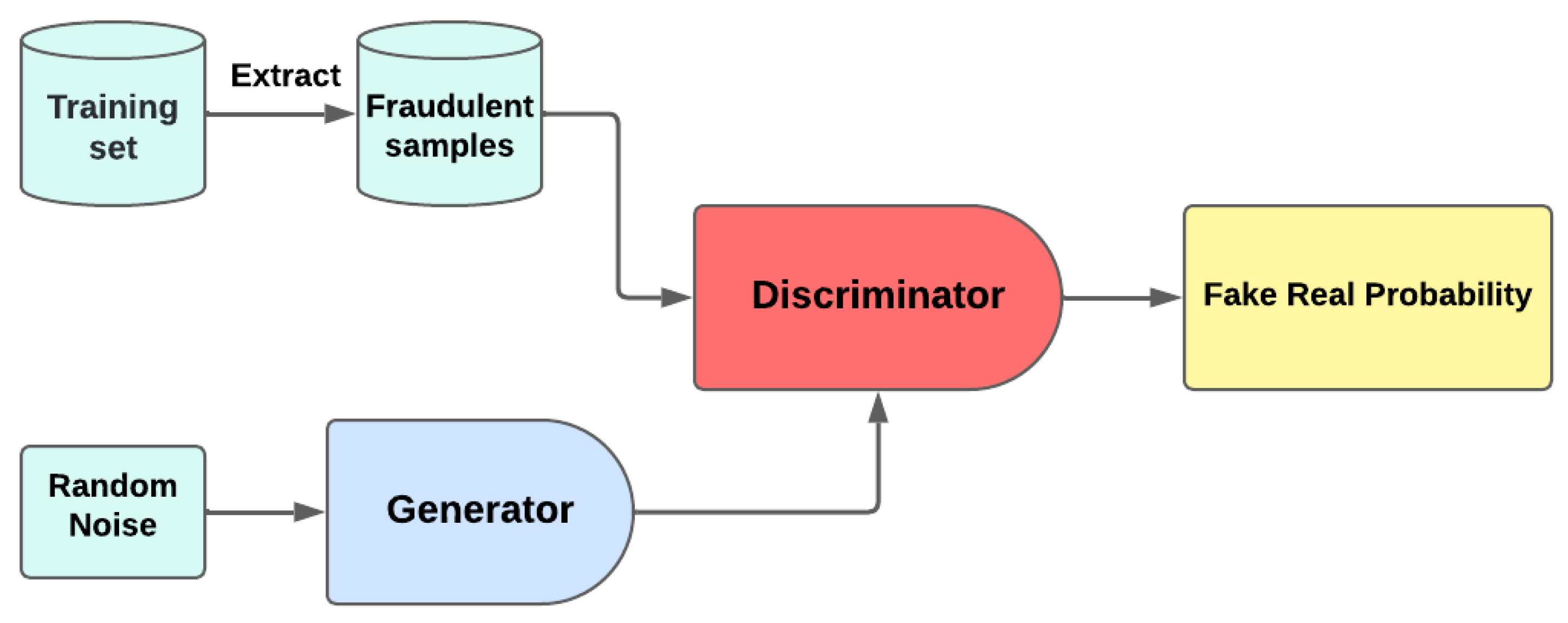
Generative modeling has recently garnered significant attention due to its effectiveness in handling diverse types of data and simulating sample behaviors [17]. Its applicability extends to various domains, including image generation and noise reduction [18]. This paper aims to leverage the capabilities of generative modeling to address the challenge of imbalanced credit card fraud detection. Specifically, we propose several models: an Autoencoder, a Variational Autoencoder (VAE), a Generative Adversarial Network (GAN), and a hybrid architecture that combines a GAN with an Autoencoder. These techniques are used for data augmentation by exploiting their ability to mimic synthetic datasets. The choice of these models is justified by their proven effectiveness in generating synthetic images and tabular datasets across various fields.

To evaluate the proposed solutions, we conducted extensive experiments using a real-world credit card dataset. We utilized various standard evaluation metrics and introduced a new metric, the Balanced Fraud Detection Score (BFDS), which combines these metrics for more accurate results and to identify the best-performing methods. Our contributions can be summarized as follows:

• Proposal of Machine Learning and deep learning Models: Several advanced machine learning and deep learning models are proposed for detecting fraudulent transactions.
• Generative Models for Handling Imbalanced Learning: To address the issue of class imbalance, we propose multiple generative models to create synthetic fraudulent samples based on historical datasets, including Autoencoders, Variational Autoencoders (VAEs), Generative Adversarial Networks (GANs), and a hybrid model combining GANs with Autoencoders. These models aim to balance the dataset and improve the detection of rare fraudulent transactions.
• Introduction of a New Evaluation Metric: We introduce a novel metric called the Balanced Fraud Detection Score (BFDS) that combines accuracy, precision, sensitivity, G-mean, and specificity to provide a comprehensive assessment of model performance.
• Empirical Validation and Comparison: Extensive experiments are conducted using a real-world credit card dataset. The results demonstrate the effectiveness of our generative modeling solutions in classifying transactions and highlight their superior performance compared to traditional methods like SMOTE and ADSYN based on the BFDS metric.

These efforts aim to advance the field of fraud detection by providing innovative solutions to class imbalance and enhancing the performance of detection systems.

Our work is organized as follows: Section 2 reviews the related work, Section 3 provides background information on the proposed model, Section 4 discusses the methodology and the materials used, Section 5 presents the experimental evaluation of our approach, and Section 6 concludes the paper and outlines our future research plans

2. Related Work

In the literature, numerous solutions have been proposed for maximizing the detection of fraudulent transactions using a variety of approaches centered on machine learning (ML) and deep learning (DL) models. To enhance these models, several strategies have been developed, including the use of statistical processes, mathematical theories, and optimization techniques such as metaheuristic algorithms [19,20] and Bayesian optimization [21]. Additionally, various methods have been proposed to handle imbalanced learning. In the rest of this section, we provide a critical review of some significant works that aim to detect fraudulent transactions effectively and with higher accuracy.

In a recent study on imbalanced classification [22], a novel approach called the clustering-based noisy-sample-removed undersampling scheme (NUS) is introduced to address the challenges faced in applications like credit card fraud detection (CCFD) and defective part identification. The study highlights the difficulties classifiers encounter due to noisy samples in both majority and minority classes. The NUS technique begins by clustering majority-class samples and then utilizes the Euclidean distance from cluster centers to define hyperspheres, identifying and excluding noisy samples. This method is applied to both majority and minority classes to enhance the classifier’s performance. The effectiveness of NUS is validated by integrating it with basic classifiers such as Random Forest (RF), Decision Tree (DT), and Logistic Regression (LR) and comparing it with seven other undersampling, oversampling, and noisy-sample-removed methods. The experiments, conducted on 13 public datasets and three real e-commerce transaction datasets, demonstrate that NUS significantly improves the performance of existing classifiers. In another paper [23], the researchers highlight the significant impact of fraud on businesses and individuals globally, where millions of US dollars are lost annually. With the surge in online transactions, credit cards have become a prevalent payment method, but they have also increased opportunities for fraudulent activities. Furthermore, the paper addresses the critical issue of data imbalance in machine learning models used for fraud detection, as fraudulent transactions constitute only a small percentage of the total data. This imbalance can severely hinder the performance of classifiers. To tackle this, the study explores various data augmentation techniques and introduces a novel model called K-means Convolutional Generative Adversarial Network (K-CGAN), which is specifically designed for credit card fraud detection. Additionally, they evaluate the effectiveness of different augmentation techniques, including B-SMOTE, K-CGAN, and SMOTE, using major classification techniques. The findings indicate that K-CGAN achieves the highest precision, recall, F1 score, and accuracy, outperforming other methods and significantly enhancing the detection of fraudulent transactions.

In [24], they focused on the importance of accurately classifying fraudulent transactions to protect customers. Using machine learning methodologies, the study tested various models, finding XGBoost to perform well with a precision score of 0.91 and an accuracy score of 0.99. To address the dataset’s imbalance, several sampling techniques were applied, with Random Oversampling emerging as the most effective, achieving a precision and accuracy score of 0.99 with XGBoost. The study emphasizes the significance of data-balancing methods in improving the performance of fraud detection models. Otherwise, Ibomoiye et al. [25] tackle the challenges of credit card fraud detection by addressing the issues posed by dynamic shopping patterns and class imbalance. They propose a robust deep learning approach, utilizing Long Short-Term Memory (LSTM) and Gated Recurrent Unit (GRU) neural networks as base learners in a stacking ensemble framework, with a Multilayer Perceptron (MLP) serving as the meta-learner. To manage the class imbalance problem, the study employs the SMOTE-ENN method. As a result, they achieve a sensitivity of 1.000 and a specificity of 0.997, outperforming other commonly used machine learning classifiers and methods. This research underscores the potential of combining advanced deep learning techniques with data balancing strategies to improve credit card fraud detection systems. In addition, ref. [26] proposes a two-stage framework that uses a deep Autoencoder for representation learning, followed by supervised deep learning techniques for fraud detection. This approach significantly improves the performance of deep learning classifiers compared to those trained on original data and other methods like PCA. The findings highlight the effectiveness of this advanced method in enhancing fraud detection systems.

Likewise, the authors in [27] proposed a framework called HNN-CUHIT that combines a hybrid neural network with a clustering-based undersampling technique, leveraging identity and transaction features. They evaluated their solution on a real dataset from a city bank during the SARS-CoV-2 pandemic in 2020. As a result, the proposed solution outperforms traditional models such as Logistic Regression, Random Forest, and CNN, particularly in handling imbalanced class distributions by achieving the best F1 score in fraud detection, highlighting its superior performance in identifying fraudulent transactions. This innovative approach offers a valuable contribution to improving fraud detection in the financial sector. Furthermore, the study [28] proposes federated learning frameworks, such as TensorFlow Federated and PyTorch. Their solution aims to enhance detection across banks without sharing sensitive data. They compare individual and hybrid resampling techniques, which prove that Random Forest classifiers outperform other models, achieving the best performance metrics. The PyTorch framework yields higher prediction accuracy for federated learning models, though with increased computational time, highlighting its effectiveness in handling skewed datasets. In addition, the study [29] tackles the challenge of acquiring labeled datasets, particularly in highly class-imbalanced domains like credit card fraud detection. It introduces a novel methodology using Autoencoders to synthesize class labels for such data. This approach minimizes the need for expert input by leveraging an error metric from the Autoencoder to create new binary class labels. These labels are then used to train supervised classifiers for fraud detection. Conducted experiments demonstrate that the synthesized labels are of high quality, significantly improving classifier performance as measured by the area under the precision–recall curve. The study also shows that increasing the proportion of positive-labeled instances enhances classifier performance, effectively addressing class imbalance concerns. In [30], the authors focus on developing a real-time fraud detection framework that can adapt to the constantly changing fraud characteristics, handle the class imbalance, and complete separation issues inherent in fraud data. The proposed solution includes a novel approach to managing non-stationary changes in transaction patterns and a robust fuzzy logistic regression model to tackle class imbalance and separation problems. This methodology improves model training efficiency and maintains high specificity and sensitivity, even with small sample sizes. The framework achieves an accuracy greater than 0.99 in identifying fraudulent and non-fraudulent transactions, outperforming other machine learning and fraud detection methods. The enhanced classification performance ensures better precision in detecting fraudulent transactions, reduces false positives, and minimizes financial losses while increasing customer satisfaction. Otherwise, Asma Cherif et al. [31] propose a new solution based on Graph Neural Networks (GNNs) for credit card fraud detection. They focus on selecting relevant features and designing a model to capture the relationships between entities like merchants and customers. Their novel encoder–decoder-based GNN model, enhanced with a graph converter and batch normalization, showed promising results on a large-scale dataset, outperforming other models in precision, recall, and F1 score.

In this paper, we aim to improve the detection of fraudulent transactions by addressing the imbalance issue through advanced generative modeling techniques. Unlike traditional methods, which often struggle with the sparse and imbalanced nature of fraudulent transaction data, our approach utilizes Variational Autoencoders (VAEs), Autoencoders, Generative Adversarial Networks (GANs), and a hybrid GAN-Autoencoder model. These models are adept at generating synthetic fraudulent samples, thereby enriching the dataset and enhancing the model’s ability to detect fraud. The efficacy of our approach is underscored by its demonstrated success in generating realistic synthetic data, as evidenced by its performance in related fields such as image and text generation. This innovative use of deep learning architectures ensures a more robust and accurate detection system, which is capable of adapting to the evolving patterns of fraudulent behavior. However, our approach has certain limitations. First, the quality of synthetic samples heavily depends on the proper tuning of hyperparameters, which can be computationally intensive. Second, the generated synthetic data may not fully capture rare or highly complex fraudulent patterns, potentially limiting the model’s generalization to unseen cases.

Table 1. The Summary of the related work.

Ref.	Proposed Solution	Metrics	Key Findings	Limitations
[22]	Clustering-based Noisy-Sample-Removed Undersampling (NUS)	Precision, Recall, F1 Score, Accuracy	Enhances classifier performance on noisy samples	Limited to datasets with clear clusters
[23]	K-means Convolutional GAN (K-CGAN)	Precision, Recall, F1 Score, Accuracy	Achieves highest metrics, superior fraud detection	High computational complexity
[24]	XGBoost with Random Oversampling	Precision, Accuracy	High precision and accuracy, effective handling of class imbalance	May overfit on minority class
[25]	LSTM and GRU in Stacking Ensemble with MLP	Sensitivity, Specificity	Achieves sensitivity of 1.000 and specificity of 0.997	Complex model, requiring extensive tuning
[26]	Deep Autoencoder for Representation Learning	Precision, Recall, F1 Score	Improves deep learning classifier performance	Limited generalization to non-financial data
[27]	HNN-CUHIT Framework	F1 Score	Outperforms traditional models, effective in imbalanced data handling	Requires specific data types and features
[28]	Federated Learning Frameworks	Prediction Accuracy	High accuracy with PyTorch, effective for federated learning	Increased computational time
[29]	Autoencoders for Synthesizing Class Labels	AUPRC (Area Under Precision-Recall Curve)	Improves classifier performance in class-imbalanced domains	Dependence on quality of synthesized labels
[30]	Real-time Fraud Detection with Fuzzy Logistic Regression	Accuracy, Specificity, Sensitivity	High accuracy (>0.99), handles class imbalance	Complex real-time adaptation
[31]	Graph Neural Networks (GNNs) for Feature Selection	Precision, Recall, F1 Score	Outperforms other models in precision, recall, and F1 score	High computational cost

provides a detailed description of the cited works.

3. Generative Models

Generative models are a type of deep learning architecture used to capture the underlying structure of data and generate synthetic data by simulating the distribution of the real data. Initially popularized for image generation due to their remarkable results, these models have garnered significant interest from researchers exploring new applications, such as dimensionality reduction and feature selection [32]. In this paper, we leverage the capabilities of generative models to address the issue of data imbalance in our dataset. Generally, this approach works as follows: given a training set $X_{\mathrm{train}}$ and a set of parameters $\theta$, a model can be constructed to estimate the probability distribution of the data. The likelihood is the probability that the model assigns to the training data for a dataset containing m samples of $x^{\left(i\right)}$:

$$\prod _{i=1}^m{p}_{\mathrm{model}}(x^{\left(i\right)};\theta )$$

(1)

The maximum likelihood method provides a way to compute the parameters $\theta$ that can maximize the likelihood of the training data [33]. To simplify the optimization, we take the logarithm of the likelihood in Equation (1) to express the probabilities as a sum rather than a product:

$${\theta }^{*}=arg\underset{\theta }{max}\sum _{i=1}^{m}log{p}_{\mathrm{model}}(x^{\left(i\right)};\theta )$$

(2)

If the true data distribution $p_{\mathrm{data}}$ lies within the family of distributions represented by $p_{\mathrm{model}}(x;\theta )$, the model can accurately approximate $p_{\mathrm{data}}$. However, in practice, the true distribution is not accessible, and only the training data are available for modeling [34]. Thus, the models must define their density function and find the $p_{\mathrm{model}}(x;\theta )$ that maximizes the likelihood. Generative models produce synthetic data by learning the probability distribution of the observed data and generating new samples from this learned distribution. The process typically involves two key components:

1.

Latent Variables: These are unobserved variables that capture the underlying factors of variation in the data. Let $\mathbf{z}$ represent a vector of latent variables, which are typically sampled from a simple prior distribution $p\left(\mathbf{z}\right)$. This prior is often chosen to be a standard normal distribution, i.e., $\mathbf{z}\sim \mathcal{N}(\mathbf{0},\mathbf{I})$.

2.

Generative Function: This function, parameterized by $\theta$, maps the latent variables $\mathbf{z}$ to the data space. The generative process can be expressed as $\mathbf{x}=G(\mathbf{z};\theta )$, where G is a neural network or another function that transforms the latent space into the data space, generating synthetic data samples $\mathbf{x}$.

The objective of training a generative model is to approximate the true data distribution $p_{\mathrm{data}}\left(\mathbf{x}\right)$ by learning the model distribution $p_{\mathrm{model}}\left(\mathbf{x}\right)$. This involves optimizing the model parameters $\theta$ such that the synthetic data distribution $p_{\mathrm{model}}\left(\mathbf{x}\right)$ closely matches the real data distribution. Meanwhile, generative models are powerful tools for data generation, but their application to imbalanced data problems comes with inherent challenges, particularly mode collapse and instability during training. Mode collapse occurs when the generator learns to produce a limited set of outputs, failing to capture the full diversity of the target distribution, which can undermine the quality of the synthetic data generated for the minority class. Additionally, the adversarial nature of those models can lead to training instability, where the generator and discriminator fail to converge, resulting in poor-quality synthetic samples. In the rest of this section, we describe the proposed models for handling the imbalance issue.

3.1. Autoencoder (AE)

Autoencoder is an unsupervised machine learning neural network model designed to learn efficient representations of input data, often for purposes such as dimensionality reduction or feature extraction [35]. The Autoencoder operates by encoding the input data into a lower-dimensional representation (encoding) using an encoder and then reconstructing the data back to their original forms (decoding) using a decoder, all while minimizing the reconstruction error [36].

As we can see from Figure 2, the Autoencoder architecture consists of two main components:

1.

Encoder: The encoder compresses the input data into a lower-dimensional space, creating a new representation known as the code or bottleneck [37]. The encoder is represented as a function f that maps the input $X_i$ to the code layer $h_i$, i.e., $h_i=f\left(X_i\right)$. This process is critical for dimensionality reduction and feature extraction.

2.

Decoder: The decoder reconstructs the data from the lower-dimensional code layer back to the original input space. The function g takes the code layer $h_i$ and produces the reconstructed output ${\tilde{X}}_i$, i.e., ${\tilde{X}}_i=g\left(h_i\right)$.

The reconstruction loss measures the difference between the input and the output, serving as an objective function to be minimized during training. This loss, often calculated using mean squared error or binary cross-entropy, ensures that the output ${\tilde{X}}_i$ closely resembles the original input $X_i$. The training objective can be formulated as

$${\mathrm{Argmin}}_{f,g}\mathrm{Loss}(X_i,{\tilde{X}}_i)$$

(3)

where the loss function measures the dissimilarity between the input $X_i$ and the reconstructed output ${\tilde{X}}_i$. In this paper, we used an Autoencoder architecture to balance our credit card dataset. The architecture and the algorithm employed are described in detail in Algorithm 1.

In this study, the hyperparameters for this Autoencoder were carefully chosen to balance model complexity, prevent overfitting, and improve the model’s ability to capture meaningful features of fraudulent samples. The model uses an input/output layer with 30 dimensions corresponding to the dataset’s features. The encoder reduces dimensionality through three hidden layers (64, 32, and 8 units) with ReLU activation, addressing vanishing gradient issues and improving convergence. Batch normalization stabilizes training, while dropout rates of 0.2 and 0.3 prevent overfitting. The symmetric decoder structure aids in effective data regeneration, and the final sigmoid output layer is suitable for binary classification. The Adam optimizer with a learning rate of 0.001 ensures efficient training, and the model is trained for 100 epochs with a batch size of 32 to balance convergence speed and computational cost. Shuffling the data during training enhances generalization by reducing the impact of data ordering.

Algorithm 1 Autoencoder Training

Require:  $fraud\_samples$, Number of epochs $epochs$, Encoding dimension $encoding\_dim$ Ensure:  Trained Autoencoder, encoder, and decoder models 1:   $input\_dim\leftarrow \mathrm{Number}\mathrm{of}\mathrm{columns}\mathrm{in}fraud\_samples$ 2:   Define Encoder Model: 3:      Input layer with shape $(30,)$ 4:      Dense layer with 64 units and activation function ‘relu’ 5:      BatchNormalization 6:      Dropout with rate 0.2 7:      Dense layer with 32 units and activation function ‘relu’ 8:      BatchNormalization 9:      Dropout with rate 0.3 10:    Dense layer with 8 units and activation function ‘relu’ 11: Define Decoder Model: 12:    Input layer with shape $(8,)$ 13:    Dense layer with 32 units and activation function ‘relu’ 14:    BatchNormalization 15:    Dropout with rate 0.3 16:    Dense layer with 64 units and activation function ‘relu’ 17:    BatchNormalization 18:    Dropout with rate 0.2 19:    Dense layer with 30 units and activation function ‘sigmoid’ 20: Define Autoencoder Model: 21:    Connect encoder and decoder 22:    Compile with optimizer Adam(learning rate = 0.001) and loss function binary_crossentropy 23: Fit the Autoencoder: 24:    Train with $fraud\_samples$ for 100 epochs and batch size 32, shuffle = True 25: return Encoder, Decoder

3.2. Variational Autoencoder (VAE)

In this paper, we utilized a Variational Autoencoder architecture to balance our credit card dataset. VAEs, introduced by Kingma et al. [38], extend traditional Autoencoders by incorporating variational inference, a statistical technique for approximating complex distributions. VAEs are generative models that use Variational Bayes Inference to model data generation through a probabilistic distribution. Unlike traditional Autoencoders, VAEs include an additional sampling layer along with the encoder and decoder layers [39]. During training, the input data are encoded as a distribution over the latent space, and the latent vector is sampled from this distribution [2]. This latent vector is then decoded, and the reconstruction error is computed and backpropagated through the network as described in Figure 3.

Probabilistically, a VAE consists of a latent representation z, drawn from a prior distribution $p\left(z\right)$, and the data point x, drawn from a conditional likelihood distribution $p(x\mid z)$, which is referred to as the probabilistic decoder. This can be expressed as follows:

$$p(x,z)=p(x\mid z)p\left(z\right)$$

(4)

The model’s inference is examined by computing the posterior of the latent vector using Bayes’ theorem, as shown in the equation below:

$$p(z\mid x)={\displaystyle \frac{p(x\mid z)p\left(z\right)}{p\left(x\right)}}$$

(5)

Using any distribution variant, such as Gaussian, variational inference can approximate the posterior. The reliability of this approximation can be assessed through the Kullback–Leibler divergence, which measures the information loss during approximation. The architecture and algorithm used for the VAE implementation in our study are detailed in Algorithm 2. This algorithm outlines the training process for a VAE on fraudulent transaction samples, with carefully chosen hyperparameters to balance model complexity, prevent overfitting, and enhance the model’s ability to capture meaningful representations. The encoder architecture, with hidden layers of 64 and 32 units, reduces the data dimensionality, capturing complex patterns without overfitting. ReLU activation is used to mitigate the vanishing gradient problem and accelerate convergence, while batch normalization stabilizes training and improves generalization. Dropout rates of 0.2 and 0.3 are applied to prevent overfitting by randomly deactivating neurons during training. The encoder outputs the mean ($\mu$) and log-variance ($log\left({\sigma }^2\right)$) for stochastic sampling, allowing the model to effectively learn from the data. The decoder mirrors the encoder structure for symmetric data reconstruction, with a sigmoid output layer suitable for binary classification. The loss function combines binary cross-entropy for reconstruction and KL divergence for regularization, promoting both accurate reconstruction and a structured latent space. The model is trained using the Adam optimizer with a learning rate of 0.001 for efficient training, for 100 epochs with a batch size of 32 to balance convergence speed and computational cost.

3.3. Generative Adversarial Network (GANs)

Generative Adversarial Networks are a class of unsupervised generative models that consist of two competing neural networks: a generator and a discriminator [40]. The generator’s primary role is to produce new data samples (fake data) that closely mimic real data distribution, aiming to deceive the discriminator. Meanwhile, the discriminator’s task is distinguishing between genuine and generated samples, providing feedback to improve the generator’s output. Figure 4 describes the main steps of a GAN. This adversarial training process continues until the generator produces data that are nearly indistinguishable from the real dataset, enhancing the model’s ability to capture complex data distributions. The competition between these networks drives both to improve iteratively, leading to the generation of high-quality synthetic data. GANs have shown remarkable success across various domains, including image synthesis, data augmentation, and anomaly detection.

The basic architecture of a GAN, often referred to as a vanilla GAN, involves the following components:

1.

Generator: The generator network takes a random noise vector as input and generates fake data. Its goal is to produce data that are as close as possible to real data samples. The generator does not have direct access to the real data; it learns to create realistic data by interacting with the discriminator [41].

2.

Discriminator: The discriminator network receives both real data and the data generated by the generator. It classifies these inputs as real or fake using a sigmoid activation function and binary cross-entropy loss. The discriminator is trained to distinguish between the real and generated data, providing feedback to the generator on how well it is performing [42].

Algorithm 2 Variational Autoencoder (VAE) Training

Require:  $fraud\_samples$, Number of epochs $epochs$, Latent dimension $latent\_dim$ Ensure:  Trained VAE, encoder, and decoder models 1:   $input\_dim\leftarrow \mathrm{Number}\mathrm{of}\mathrm{columns}\mathrm{in}fraud\_samples$ 2:   Define Encoder Model: 3:      Input layer with shape $(30,)$ 4:      Dense layer with 64 units and activation function ‘relu’ 5:      BatchNormalization 6:      Dropout with rate 0.2 7:      Dense layer with 32 units and activation function ‘relu’ 8:      BatchNormalization 9:      Dropout with rate 0.3 10:    Dense layer with 8 units for mean ($\mu$) 11:    Dense layer with 8 units for log-variance ($log\left({\sigma }^2\right)$) 12:    Sampling layer using $z=\mu +\sigma ·ϵ$, where $ϵ\sim \mathcal{N}(0,1)$ 13: Define Decoder Model: 14:    Input layer with shape $(8,)$ 15:    Dense layer with 32 units and activation function ‘relu’ 16:    BatchNormalization 17:    Dropout with rate 0.3 18:    Dense layer with 64 units and activation function ‘relu’ 19:    BatchNormalization 20:    Dropout with rate 0.2 21:    Dense layer with 30 units and activation function ‘sigmoid’ 22: Define VAE Model: 23:    Connect encoder and decoder 24:    Define VAE loss as reconstruction loss (binary cross-entropy) plus KL divergence: 25:    $\mathcal{L}\left(x\right)={\mathbb{E}}_{q\left(z\right|x)}[logp\left(x\right|z)]-D_{KL}\left(q\left(z\right|x)\right|\left|p\left(z\right)\right)$ 26:    Compile with optimizer Adam(learning rate = 0.001) 27: textbfFit the VAE: 28:    Train with $fraud\_samples$ for 100 epochs and batch size 32, shuffle=True 29: return Encoder, Decoder

The generator and discriminator are trained together in a competitive process known as a minimax game, where the generator tries to maximize the probability that the discriminator mistakes fake data for real data, while the discriminator tries to minimize this probability. This can be expressed mathematically as

$$\underset{G}{min}\underset{D}{max}V(D,G)={\mathbb{E}}_{x\sim p_{\mathrm{data}}\left(x\right)}[logD\left(x\right)]+{\mathbb{E}}_{z\sim p_z\left(z\right)}[log(1-D\left(G\left(z\right)\right))]$$

(6)

where $\mathbb{E}$ denotes the expected value, $p_{\mathrm{data}}\left(x\right)$ represents the distribution of real data, and $p_z\left(z\right)$ represents the distribution of the noise input to the generator. During training, the generator and discriminator engage in a dynamic process where the generator attempts to improve its ability to produce realistic data while the discriminator continually refines its ability to distinguish real data from fake data. This iterative process continues until the discriminator can no longer reliably differentiate between real and fake data, indicating that the generator has succeeded in producing highly realistic data. The feedback loop provided by the discriminator is crucial for the generator’s learning process. After each batch of training, backpropagation is used to update the weights of both the generator and discriminator networks, optimizing their performance. Algorithm 3 shows our proposed architecture of the GAN model used to address the imbalance issue. The choice of hyperparameters in the GAN training algorithm is made to optimize both model performance and stability. The generator’s architecture uses progressively smaller layers (128, 64, 50, 40, and 15 units) to effectively map a high-dimensional latent space to the target data distribution. The larger initial layers (128 and 64 units) capture more complex features, while the smaller layers reduce the dimensionality to match the output data. ReLU activation functions are employed throughout the generator to mitigate the vanishing gradient problem and speed up convergence. Dropout is set to 0.5 to regularize the model and prevent overfitting by randomly deactivating half of the units during training. Batch normalization is applied to stabilize training by normalizing layer inputs, ensuring more consistent gradients. In the discriminator, the choice of 128, 64, and 32 units, along with LeakyReLU activations, allows the model to effectively distinguish between real and fake data while mitigating the risk of dying neurons. Dropout is similarly set to 0.5 in the discriminator to avoid overfitting, and the use of binary cross-entropy loss ensures the proper evaluation of fake and real data. The Adam optimizer with a learning rate of 0.001 is selected for both models to ensure efficient training and prevent the instability often seen with other optimizers in GAN training.  

3.4. AE-GAN

AE-GAN is a hybrid approach that combines an Autoencoder and a Generative Adversarial Network to effectively address the imbalance issue in credit card datasets. This combination leverages the strengths of both models to improve the quality and diversity of synthetic data, which is crucial for training robust fraud detection systems, as shown in Figure 5. The process is outlined as follows:

1.

Extract fraudulent samples from the training set.

2.

Pass these samples through an Autoencoder (AE) to encode the data into a lower-dimensional space.

3.

Apply Principal Component Analysis (PCA) to reduce the dimensionality of the encoded data to 15 features.

4.

Train a Generative Adversarial Network (GAN) using the PCA-reduced data. The GAN consists of a generator and a discriminator.

5.

Use the generator to produce synthetic features based on the reduced data.

6.

Pass these generated features through the decoder of the Autoencoder to reconstruct the synthetic data.

Algorithm 3 GAN Training

Require:  $fraud\_samples$, Number of epochs $epochs$ Ensure:  Trained generator model 1:   Define Generator Model: 2:   Create a sequential model with: 3:      Dense layer with 128 units, activation ‘relu’, input_dim=15 4:      Dropout with rate 0.5 5:      BatchNormalization 6:      Dense layer with 64 units, activation ‘relu’ 7:      Dropout with rate 0.5 8:      BatchNormalization 9:      Dense layer with 50 units, activation ‘relu’ 10:    Dense layer with 40 units, activation ‘relu’ 11:    Dense layer with 15 units 12: Define Discriminator Model: 13: Create a sequential model with: 14:    Dense layer with 128 units, input_dim=15 15:    Dropout with rate 0.5 16:    LeakyReLU with alpha=0.2 17:    Dense layer with 64 units 18:    Dropout with rate 0.5 19:    LeakyReLU with alpha=0.2 20:    Dense layer with 32 units 21:    Dropout with rate 0.5 22:    Dense layer with 1 unit, activation ‘sigmoid’ 23: Define loss function BinaryCrossentropy() 24: Define optimizer $\mathrm{Adam}(\mathrm{learning}\_\mathrm{rate}=0.001)$ 25: for epoch = 1 to epochs do 26:     Train Discriminator: 27:        Compute loss on real data and fake data 28:        Update discriminator weights 29:     Train Generator: 30:        Generate fake data 31:        Compute loss based on discriminator output 32:        Update generator weights 33: end for 34: return Trained generator

Figure 5. Autoencoder and GAN-based synthetic data generation.

Figure 5. Autoencoder and GAN-based synthetic data generation.

Algorithm 4 describes the main steps of the AE-GAN model. 

Algorithm 4 Autoencoder and GAN-Based Synthetic Data Generation

1: Input: Fraudulent samples ${\mathbf{X}}_{\mathrm{fraud}}\in {\mathbb{R}}^{m\times n}$, where m is the number of samples and n is the number of features. 2: Train an Autoencoder on ${\mathbf{X}}_{\mathrm{fraud}}$ to obtain the encoder $E:{\mathbb{R}}^n\to {\mathbb{R}}^d$ and decoder $D:{\mathbb{R}}^d\to {\mathbb{R}}^n$, where d is the dimensionality of the encoded space. 3: Apply Principal Component Analysis (PCA) to ${\mathbf{X}}_{\mathrm{fraud}}$ to reduce the dimensionality to 15 features, resulting in ${\mathbf{X}}_{\mathrm{PCA}}\in {\mathbb{R}}^{m\times 15}$. 4: Train a Generative Adversarial Network (GAN) on ${\mathbf{X}}_{\mathrm{PCA}}$ to obtain the generator $G:{\mathbb{R}}^z\to {\mathbb{R}}^{15}$ and discriminator $D_{\mathrm{GAN}}$. 5: Use the encoder E to encode the original fraud samples ${\mathbf{X}}_{\mathrm{fraud}}$ into 15-dimensional features $\mathbf{Z}=E\left({\mathbf{X}}_{\mathrm{fraud}}\right)\in {\mathbb{R}}^{m\times 15}$. 6: Generate synthetic data ${\mathbf{Z}}_{\mathrm{syn}}=G\left(\mathbf{Z}\right)\in {\mathbb{R}}^{m\times 15}$. 7: Decode ${\mathbf{Z}}_{\mathrm{syn}}$ using the decoder D to obtain synthetic data with 30 features, ${\mathbf{X}}_{\mathrm{syn}}=D\left({\mathbf{Z}}_{\mathrm{syn}}\right)\in {\mathbb{R}}^{m\times n}$. 8: Output: Synthetic data ${\mathbf{X}}_{\mathrm{syn}}$.

4. Methodology and Materials

4.1. Dataset

The dataset utilized for our experiments is a publicly available and widely referenced credit card fraud detection dataset originally introduced in [43]. This dataset was created through a collaboration between Worldline, a major payment processing company, and the Université Libre de Bruxelles. It encompasses over 280,000 European credit card transactions recorded between 1 September and 30 September 2013, making it a unique resource as the only publicly available dataset that represents real-world credit card usage patterns. The dataset consists of 30 independent features, anonymized using principal component analysis (PCA). These features include “Amount”, “Time”, and “V1” through “V28.” The “V” features are the result of the PCA transformation applied to anonymize the data. In this dataset, transactions are labeled as either genuine or fraudulent, serving as ground truth for calculating the performance of supervised learning models. However, it is important to note that our method disregards these labels during the synthesis of new class labels. As is common in fraud detection datasets, this dataset is highly imbalanced, with genuine transactions vastly outnumbering fraudulent ones. The detailed breakdown of the dataset’s characteristics is presented in

Table 2. Credit card fraud detection dataset class characteristics.

Minority	Majority	Total	Minority Imbalance	Features
492	284,315	284,807	0.1727%	29

, with 492 fraudulent and 284,315 genuine transactions, resulting in an overall count of 284,807 transactions. A significant challenge in the domain of fraud detection is obtaining accurate class labels for transactions. Privacy concerns necessitate the anonymization or removal of personally identifiable information, making the creation of publicly available datasets with real-world examples challenging. The dataset we use has undergone such anonymization, ensuring that it is a valuable resource for public research while safeguarding privacy. This particular dataset, to the best of our knowledge, remains the only publicly accessible dataset for credit card fraud detection analysis, thus, our research exclusively focuses on it.

4.2. Evaluation Metrics

In this study, we evaluate the classification performance of supervised learners using a range of performance metrics. These include accuracy, precision, sensitivity, specificity, G-mean, and F-measure. These metrics provide a comprehensive evaluation of the classifiers’ ability to distinguish between fraudulent and legitimate transactions. For binary classification problems, such as fraud detection, it is conventional to use a confusion matrix to summarize the classification results. The confusion matrix consists of true positives (TPs), false positives (FPs), false negatives (FNs), and true negatives (TNs). These values are crucial for calculating the following metrics:

• Accuracy: This metric measures the overall correctness of the model by comparing the number of correct predictions (both true positives and true negatives) to the total number of cases. It is calculated as follows:

  $$\mathrm{Accuracy}={\displaystyle \frac{TP+TN}{TP+FP+FN+TN}}$$

  (7)
• Precision: Precision indicates the accuracy of positive predictions and is calculated as follows:

  $$\mathrm{Precision}={\displaystyle \frac{TP}{TP+FP}}$$

  (8)
• Sensitivity (recall or true positive rate): This metric measures the ability of the model to identify true positive cases. It is calculated as follows:

  $$\mathrm{Sensitivity}={\displaystyle \frac{TP}{TP+FN}}$$

  (9)
• Specificity: Specificity measures the proportion of true negatives correctly identified by the model and is calculated as follows:

  $$\mathrm{Specificity}={\displaystyle \frac{TN}{TN+FP}}$$

  (10)
• G-mean: The G-mean metric is a geometric mean of sensitivity and specificity. It provides a balance between these two metrics and is particularly useful in imbalanced datasets:

  $$\mathrm{G}-\mathrm{mean}=\sqrt{\mathrm{Sensitivity}\times \mathrm{Specificity}}$$

  (11)
• F-measure: The F-measure, or F1 score, is the harmonic mean of precision and recall. It provides a single score that balances the importance of both metrics:

  $$\mathrm{F}-\mathrm{measure}=2\times {\displaystyle \frac{\mathrm{Precision}\times \mathrm{Recall}}{\mathrm{Precision}+\mathrm{Recall}}}$$

  (12)

Traditional metrics like accuracy can be misleading due to the imbalance in the dataset. For instance, a model that predicts all transactions as legitimate could still achieve high accuracy due to the overwhelming number of legitimate transactions. To address this, we also consider the G-mean and F-measure, which are better suited for evaluating models on imbalanced datasets. G-mean ensures that the classifier performs well on both classes, while F-measure balances the trade-off between precision and sensitivity. These metrics, along with the analysis of the confusion matrix, provide a comprehensive view of the classifier’s performance and its effectiveness in distinguishing between fraudulent and legitimate behaviors. This approach allows us to better understand the strengths and weaknesses of the classifiers and the impact of class imbalance on the classification results. In addition, for an accurate comparison, we created a new metric based on

Table 3. Table of metric scores with justifications.

Metric	Importance Score (1–10)	Normalized Weight	Justification
Accuracy	7	0.117	Reflects the overall performance of the model, but may not fully capture the performance on fraud detection specifically.
Precision	9	0.150	High precision means fewer false positives, which is crucial in fraud detection to avoid wrongly flagging legitimate transactions.
Recall	10	0.167	Very important as high recall ensures that most fraudulent transactions are detected, minimizing missed fraud cases.
G-Mean	8	0.133	Balances performance between classes, important for handling class imbalance in fraud detection.
Specificity	7	0.117	Indicates how well the model identifies non-fraudulent transactions; important but slightly less critical than recall.
F-Measure	9	0.150	It combines precision and recall, providing a balanced view of the model’s ability to detect fraud while minimizing false positives.

, which summarizes all the proposed metrics in this paper. This new metric, called the Balanced Fraud Detection Score (BFDS), combines key performance indicators to provide a comprehensive evaluation of the model’s effectiveness in fraud detection. The formula for calculating the BFDS is

$$\begin{array}{cc}\hfill \mathrm{BFDS}=& 0.117\times \mathrm{Accuracy}+0.150\times \mathrm{Precision}+0.167\times \mathrm{Recall}+\hfill \\ \hfill & 0.133\times \mathrm{G}-\mathrm{Mean}+0.117\times \mathrm{Specificity}+\hfill \\ \hfill & 0.150\times \mathrm{F}-\mathrm{Measure}\hfill \end{array}$$

(13)

The coefficients in the BFDS formula are designed to reflect the importance of each evaluation metric in fraud detection. Metrics like recall, precision, and F-measure are assigned higher weights due to their role in identifying fraud while minimizing errors. Recall has the highest weight, as detecting fraudulent transactions is crucial, while precision and F-measure balance false positives and overall model performance. All weights are divided by 60 to ensure that the gap between all metrics is reduced, providing a more comprehensive and accurate evaluation of performance in imbalanced datasets.

4.3. Proposed Solution

In this work, our goal is to achieve better results in detecting fraudulent transactions by leveraging oversampling techniques through generative modeling. To this end, we propose several generative models due to their strong ability to simulate the behavior of a dataset and construct similar synthetic datasets. Our solution can be described as follows: first, we apply a Random Scaler to the Amount and Time features to standardize these attributes. Next, we divide the data into training and testing sets, with 70% allocated for training and 30% for testing. After this, we apply an oversampling technique to the training set to enhance the representation of the minority class. We then train our model using the oversampled training data. Finally, we classify the testing set with the trained model and perform extensive evaluations to identify the most effective strategies for detecting fraudulent transactions. Figure 6 and Algorithm 5 show the main steps of the proposed solution.

Algorithm 5 Proposed Solution Workflow

Require:  Dataset D with features including Amount and Time Ensure:  Best model and oversampling strategy for fraud detection 1:   Step 1: Apply Random Scaler to Amount and Time features 2:   $D^{\prime }\leftarrow \mathrm{RandomScaler}\left(D\right)$ 3:   Step 2: Split the data into training and testing sets 4:   $(D_{train},D_{test})\leftarrow \mathrm{Split}(D^{\prime },70\%,30\%)$ 5:   Step 3: Apply oversampling technique to the training set 6:   $D_{train\_over}\leftarrow \mathrm{Oversample}\left(D_{train}\right)$ 7:   Step 4: Train the model on the oversampled training set 8:   $model\leftarrow \mathrm{TrainModel}\left(D_{train\_over}\right)$ 9:   Step 5: Classify the testing set using the trained model 10: $predictions\leftarrow \mathrm{Classify}(model,D_{test})$ 11: Step 6: Conduct evaluation to choose the best strategies for detecting fraudulent transactions 12: $\mathrm{Evaluate}(predictions,D_{test})$ 13: Output: Best model and oversampling strategy

5. Results and Discussion

To evaluate our proposed solution, we conducted extensive experiments using a variety of machine learning algorithms and deep learning models. The machine learning algorithms included Logistic Regression (LR), Decision Tree (DT), Random Forest (RF), Gradient Boosting (GB), XGBoost (XGB), LightGBM (LGBM), K-Nearest Neighbors (KNN), Naive Bayes (NB), AdaBoost (AB), and Bagging Classifier (BC). For deep learning, we utilized Artificial Neural Networks (ANNs), Long Short-Term Memory (LSTM) networks, and Recurrent Neural Networks (RNNs). Although LSTM and RNN models are typically used for sequential data with temporal dependencies, we employed these models to capture complex patterns and non-linear interactions within the features. Fraud detection often involves intricate relationships between variables that may not be fully captured by conventional models. By leveraging LSTM and RNN architectures, we aimed to enhance the model’s ability to identify subtle patterns indicative of fraudulent behavior, even in the absence of explicit temporal information. Additionally, our main objective is to offer a performance analysis comparing traditional machine learning models with deep learning models in detecting fraudulent transactions. These experiments aimed to assess the performance and effectiveness of our solution across various techniques and models. Figure 7, Figure 8, Figure 9, Figure 10, Figure 11, Figure 12, Figure 13 and Figure 14 show the results obtained using different resampling techniques. From these figures, we observe that the outcomes are promising, demonstrating the efficiency of our proposed methods.

Table 4. Model performance metrics using GAN.

Model	Accuracy	Specificity	Sensitivity	Precision	F-Measure	G-Mean
LR	0.999298	0.999824	0.669118	0.858491	0.752066	0.817924
DT	0.999111	0.999390	0.823529	0.682927	0.746667	0.907209
RF	0.999637	0.999930	0.816176	0.948718	0.877470	0.903393
GB	0.999473	0.999777	0.808824	0.852713	0.830189	0.899246
XGB	0.999649	0.999918	0.830882	0.941667	0.882813	0.911490
LGBM	0.999590	0.999871	0.823529	0.910569	0.864865	0.907427
KNN	0.999473	0.999859	0.757353	0.895652	0.820717	0.870199
NB	0.998408	1.000000	0.000000	0.000000	0.000000	0.000000
AB	0.999309	0.999695	0.757353	0.798450	0.777358	0.870128
BC	0.999532	0.999871	0.786765	0.906780	0.842520	0.886940
ANN	0.999380	0.999812	0.727941	0.860870	0.788845	0.853115
LSTM	0.999532	0.999871	0.786765	0.906780	0.842520	0.886940
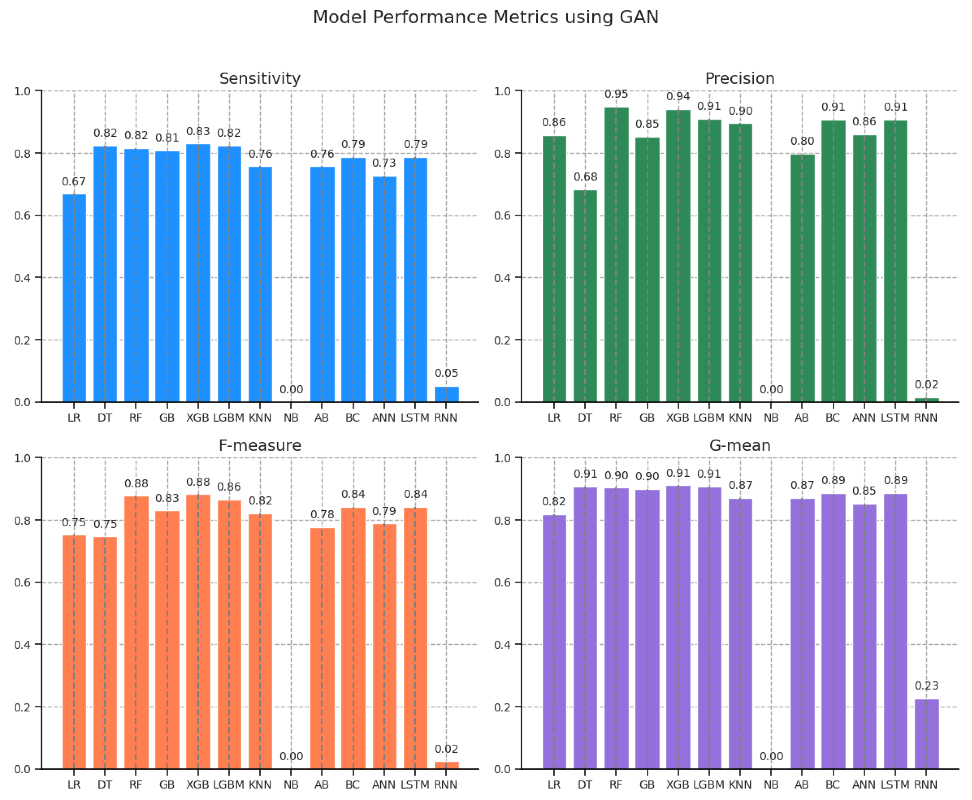
RNN	0.993551	0.995053	0.051471	0.016317	0.024779	0.226309

presents the performance metrics of various machine learning models using Generative Adversarial Networks for data augmentation. Among the evaluated models, XGB achieved the highest sensitivity (0.830882) and demonstrated strong performance across other metrics, including precision (0.941667), F-measure (0.882813), and G-mean (0.911490). RF also performed competitively with an F-measure of 0.877470 and a G-mean of 0.903393, indicating a balanced trade-off between sensitivity and specificity. LR and DT showed moderate sensitivity (0.669118 and 0.823529, respectively), with DT having a higher G-mean (0.907209) compared to LR (0.817924). Notably, the NB model performed poorly, with a sensitivity of 0.000000 and corresponding F-measure and G-mean values of 0.000000, suggesting its ineffectiveness in the given context. Additionally, advanced neural network models such as LSTM and ANN demonstrated robust performance, with LSTM matching the performance of BC in all metrics. Overall, tree-based ensemble methods (RF, XGB, and LGBM) consistently outperformed other models, reflecting their ability to capture complex data patterns effectively.

Figure 7 provides a clear visualization of the performance metrics of various models using GAN to address class imbalance. From these plots, it is evident that XGB and RF outperform other models, achieving the highest sensitivity, precision, F-measure, and G-mean. LGBM and GB exhibit strong performance, though it is slightly lower than XGB and RF. DT performs well in sensitivity but lags in precision, which affects its overall F-measure. Simpler models like LR and KNN show moderate results, with AB performing similarly. NB and RNN struggle to adapt to GAN-generated data, performing poorly across all metrics.

Table 5. Model performance metrics using AE-GAN.

Model	Accuracy	Specificity	Sensitivity	Precision	F-Measure	G-Mean
LR	0.999286	0.999836	0.654412	0.864078	0.744770	0.808891
DT	0.999111	0.999449	0.786765	0.694805	0.737931	0.886753
RF	0.999544	0.999894	0.779412	0.921739	0.844622	0.882796
GB	0.999555	0.999883	0.794118	0.915254	0.850394	0.891081
XGB	0.999649	0.999953	0.808824	0.964912	0.880000	0.899325
LGBM	0.999544	0.999836	0.816176	0.888000	0.850575	0.903351
KNN	0.999462	0.999859	0.750000	0.894737	0.816000	0.865964
NB	0.998408	1.000000	0.000000	0.000000	0.000000	0.000000
AB	0.999111	0.999695	0.632353	0.767857	0.693548	0.795085
BC	0.999532	0.999883	0.779412	0.913793	0.841270	0.882791
ANN	0.999321	0.999871	0.654412	0.890000	0.754237	0.808905
LSTM	0.999450	0.999766	0.801471	0.844961	0.822642	0.895144
RNN	0.995564	0.996659	0.308824	0.128440	0.181425	0.554790

displays the performance metrics of various machine learning models using Autoencoder–Generative Adversarial Networks (AE-GANs). Among the models, XGB achieved the best overall performance, with the highest sensitivity (0.808824), precision (0.964912), F-measure (0.880000), and a G-mean of 0.899325, indicating its superior ability to balance false positives and false negatives. LGBM also performed well, with a sensitivity of 0.816176 and an F-measure of 0.850575, reflecting its effectiveness in handling complex patterns. RF and GB achieved similar performance levels, with F-measure values of 0.844622 and 0.850394, respectively, demonstrating the robustness of ensemble-based methods. In contrast, NB again performed poorly, with sensitivity, precision, and F-measure values of 0.000000, indicating its inability to capture meaningful patterns in the AE-GAN-enhanced dataset. Neural network models such as LSTM and ANN showed moderate performance, with LSTM achieving a higher sensitivity (0.801471) and F-measure (0.822642) compared to ANN. The RNN model exhibited the weakest performance among deep learning methods, with a low sensitivity (0.308824) and an F-measure of 0.181425. Overall, tree-based ensemble methods, particularly XGB and LGBM, consistently outperformed other models, highlighting their adaptability and effectiveness when paired with AE-GAN-generated data.

Figure 8 visualizes the performance metrics of various models using AE-GAN to address class imbalance in fraud detection. XGB achieved the highest accuracy at 99.96%, with Naive Bayes (NB) showing perfect specificity but zero sensitivity, limiting its usefulness. Sensitivity was highest in XGB, LGBM, and LSTM, at around 80–81%. XGB also achieved the highest precision and F-measure, demonstrating its strong fraud detection ability. G-mean scores were highest in XGB and LGBM, reflecting their balanced performance. The RNN model showed lower performance across all metrics, particularly in sensitivity and precision, indicating its limited effectiveness.

Table 6. Model performance metrics using AE.

Model	Accuracy	Specificity	Sensitivity	Precision	F-Measure	G-Mean
LR	0.999181	0.999801	0.610294	0.830000	0.703390	0.781135
DT	0.999052	0.999414	0.772059	0.677419	0.721649	0.878411
RF	0.999579	0.999918	0.786765	0.938596	0.856000	0.886961
GB	0.999427	0.999789	0.772059	0.853659	0.810811	0.878576
XGB	0.999672	0.999965	0.816176	0.973684	0.888000	0.903409
LGBM	0.999614	0.999930	0.801471	0.947826	0.868526	0.895217
KNN	0.999462	0.999859	0.750000	0.894737	0.816000	0.865964
NB	0.998408	1.000000	0.000000	0.000000	0.000000	0.000000
AB	0.998982	0.999613	0.602941	0.713043	0.653386	0.776343
BC	0.999473	0.999859	0.757353	0.895652	0.820717	0.870199
ANN	0.999274	0.999941	0.580882	0.940476	0.718182	0.762134
LSTM	0.999415	0.999766	0.779412	0.841270	0.809160	0.882740
RNN	0.877778	0.879131	0.029412	0.000388	0.000765	0.160800

presents the performance metrics of various machine learning models using Autoencoder (AE) for feature extraction. XGB achieved the best overall performance, with the highest sensitivity (0.816176), precision (0.973684), and F-measure (0.888000), along with a G-mean of 0.903409, indicating its effectiveness in maintaining a balance between sensitivity and specificity. LGBM also performed competitively, with a sensitivity of 0.801471 and an F-measure of 0.868526, demonstrating its robustness in handling the AE-transformed data. RF followed closely with a sensitivity of 0.786765 and an F-measure of 0.856000, further confirming the strength of ensemble-based approaches. Conversely, the NB model again performed poorly, yielding sensitivity, precision, and F-measure values of 0.000000, making it unsuitable for this dataset. Neural network models displayed mixed results, with LSTM achieving better performance (F-measure of 0.809160) than ANN (0.718182), while the RNN model exhibited the weakest performance across all metrics (sensitivity of 0.029412 and F-measure of 0.000765), indicating challenges in learning from AE-transformed data. DT and Bagging Classifier (BC) showed moderate performance, with G-means of 0.878411 and 0.870199, respectively. Overall, tree-based ensemble models, especially XGB and LGBM, outperformed other models, highlighting their superior ability to extract meaningful patterns from AE-enhanced datasets.

Figure 9 visualizes the performance metrics of various models using AE to address class imbalance in fraud detection. XGB achieved the highest accuracy at 99.97%, with NB showing perfect specificity but zero sensitivity, limiting its usefulness. Sensitivity was highest in XGB and LGBM, with values of 81.6% and 80.1%, respectively. XGB also achieved the highest precision (97.37%) and F-measure, reflecting its strong fraud detection ability. G-mean scores were highest in XGB and LGBM, indicating their robustness in fraud detection. The RNN model performed poorly across all metrics, particularly in sensitivity, precision, and G-mean, highlighting its limited effectiveness in fraud detection.

Table 7. Model performance metrics with VAE.

Model	Accuracy	Specificity	Sensitivity	Precision	F-Measure	G-Mean
LR	0.930679	0.930733	0.897059	0.020229	0.039565	0.913741
DT	0.997179	0.997515	0.786765	0.335423	0.470330	0.885895
RF	0.999555	0.999871	0.801471	0.908333	0.851562	0.895191
GB	0.998151	0.998675	0.669118	0.446078	0.535294	0.817454
XGB	0.999532	0.999848	0.801471	0.893443	0.844961	0.895181
LGBM	0.999216	0.999519	0.808824	0.728477	0.766551	0.899130
KNN	0.999462	0.999859	0.750000	0.894737	0.816000	0.865964
NB	0.849256	0.850575	0.022059	0.000235	0.000466	0.136977
AB	0.992791	0.993494	0.551471	0.119048	0.195822	0.740191
BC	0.998830	0.999179	0.779412	0.602273	0.679487	0.882481
ANN	0.999462	0.999719	0.838235	0.826087	0.832117	0.915423
LSTM	0.999438	0.999824	0.757353	0.872881	0.811024	0.870184
RNN	0.995658	0.996788	0.286765	0.124601	0.173719	0.534643

shows the performance metrics of various machine learning models using Variational Autoencoder (VAE) for data augmentation. RF and XGB demonstrated the best overall performance, both achieving a sensitivity of 0.801471 and comparable F-measure values of 0.851562 and 0.844961, respectively. RF slightly outperformed XGB in terms of precision (0.908333 vs. 0.893443), suggesting it is more effective at minimizing false positives. LGBM also performed well, with a sensitivity of 0.808824 and a G-mean of 0.899130, indicating a balanced ability to detect positive instances while maintaining high specificity. Among neural network models, ANN achieved the highest sensitivity (0.838235) and F-measure (0.832117), showing its strength in handling the complex data generated by VAE. In contrast, the NB model performed the worst, with a sensitivity of 0.022059 and an F-measure of 0.000466, making it ineffective for this dataset. Logistic Regression (LR) also struggled, with a low F-measure of 0.039565 despite a relatively high G-mean (0.913741). While DT and BC delivered moderate performance, boosting-based models like GB and AB underperformed in terms of sensitivity (0.669118 and 0.551471, respectively). Overall, ensemble methods—particularly RF, XGB, and LGBM—consistently achieved superior performance, while NB and simpler models like LR were less effective in learning from VAE-augmented data.

Figure 10 shows the performance of various models using Variational Autoencoder (VAE) for fraud detection. XGB and RF excel with high accuracy, specificity, and balanced sensitivity, precision, and F-measure. LGBM also performs well, achieving high specificity and good sensitivity (80.88%) with a strong G-mean. LR and DT show good specificity but struggle with precision and F-measure, limiting their fraud detection ability. NB underperforms with low sensitivity and precision. The LSTM model demonstrates a good balance, with a high G-mean (87.02%), while the RNN model has low sensitivity and precision. XGB and RF are the top performers.

Table 8. Model performance metrics with SMOTE.

Model	Accuracy	Specificity	Sensitivity	Precision	F-Measure	G-Mean
LR	0.973409	0.973484	0.926471	0.052764	0.099842	0.949686
DT	0.997425	0.997820	0.750000	0.354167	0.481132	0.865081
RF	0.999555	0.999766	0.867647	0.855072	0.861314	0.931367
GB	0.987922	0.988031	0.919118	0.109075	0.195008	0.952952
XGB	0.999274	0.999496	0.860294	0.731250	0.790541	0.927287
LGBM	0.998432	0.998640	0.867647	0.504274	0.637838	0.930842
KNN	0.997729	0.997890	0.897059	0.403974	0.557078	0.946132
NB	0.975808	0.975957	0.882353	0.055274	0.104031	0.927976
AB	0.973702	0.973765	0.933824	0.053700	0.101559	0.953585
BC	0.998888	0.999191	0.808824	0.614525	0.698413	0.898982
ANN	0.999204	0.999402	0.875000	0.700000	0.777778	0.935135
LSTM	0.997683	0.997902	0.860294	0.395270	0.541667	0.926547
RNN	0.975212	0.975324	0.904412	0.055206	0.104061	0.939199

presents the performance metrics of various machine learning models using the Synthetic Minority Oversampling Technique (SMOTE) to address class imbalance. Among the models, Random Forest (RF) achieved the best overall performance, with a sensitivity of 0.867647, a precision of 0.855072, and an F-measure of 0.861314, highlighting its strong ability to detect minority class samples while maintaining high accuracy. XGB and ANN models also performed competitively, with XGB achieving a sensitivity of 0.860294 and an F-measure of 0.790541, while ANN recorded a sensitivity of 0.875000 and an F-measure of 0.777778, showcasing their robustness in learning from the oversampled data. LGBM achieved a similar sensitivity (0.867647) but had a lower precision (0.504274), resulting in a lower F-measure (0.637838), indicating a trade-off between detecting positive samples and minimizing false positives. In contrast, simpler models like LR and NB struggled with low precision (0.052764 and 0.055274, respectively) and F-measures (0.099842 and 0.104031, respectively), despite having relatively high sensitivity (0.926471 for LR and 0.882353 for NB), reflecting their difficulty in handling the increased complexity of the SMOTE data. DT and BC displayed moderate performance, with sensitivities of 0.750000 and 0.808824, respectively, and F-measures of 0.481132 and 0.698413. Notably, GB and AB underperformed in precision (0.109075 and 0.053700) and F-measure (0.195008 and 0.101559), reflecting their challenges in balancing false positives and false negatives. Overall, ensemble models—particularly RF, XGB, and ANN—outperformed other approaches, demonstrating their effectiveness in handling class imbalance when combined with SMOTE. Simpler models like LR, NB, and boosting methods exhibited lower precision and F-measure, making them less suitable for datasets with imbalanced classes.

The bar plots in Figure 11, representing the model performance metrics with SMOTE, showcase the accuracy, specificity, sensitivity, precision, F-measure, and G-mean of different classifiers. Random Forest (RF) stands out with consistently high values across all metrics, particularly in accuracy and specificity, emphasizing its effectiveness in detecting both fraudulent and non-fraudulent transactions. XGB and ANN also display solid performances, particularly in accuracy, specificity, and sensitivity, making them reliable choices for fraud detection. On the other hand, models like Naive Bayes (NB), AdaBoost (AB), and Logistic Regression (LR) show significant discrepancies, with low precision and F-measure, indicating challenges in identifying fraudulent transactions accurately. Likewise, K-Nearest Neighbors (KNN) and Gradient Boosting (GB) show a balance in their metrics, particularly in sensitivity, though their precision and F-measure could be improved. Overall, the plot indicates that RF, XGB, and ANN are the top performers, while models like Naive Bayes and AdaBoost need further optimization for better fraud detection.

Table 9. Model performance metrics with ADASYN.

Model	Accuracy	Specificity	Sensitivity	Precision	F-Measure	G-Mean
LR	0.908945	0.908870	0.955882	0.016447	0.032338	0.932080
DT	0.998022	0.998359	0.786765	0.433198	0.558747	0.886269
RF	0.999544	0.999789	0.845588	0.864662	0.855019	0.919462
GB	0.967429	0.967447	0.955882	0.044720	0.085442	0.961647
XGB	0.999263	0.999437	0.889706	0.715976	0.793443	0.942977
LGBM	0.997870	0.998019	0.904412	0.421233	0.574766	0.950063
KNN	0.997729	0.997890	0.897059	0.403974	0.557078	0.946132
NB	0.959903	0.959980	0.911765	0.035048	0.067501	0.935562
AB	0.943787	0.943826	0.919118	0.025422	0.049476	0.931390
BC	0.998771	0.999097	0.794118	0.583784	0.672897	0.890731
ANN	0.999181	0.999379	0.875000	0.691860	0.772727	0.935124
LSTM	0.998151	0.998335	0.882353	0.458015	0.603015	0.938554
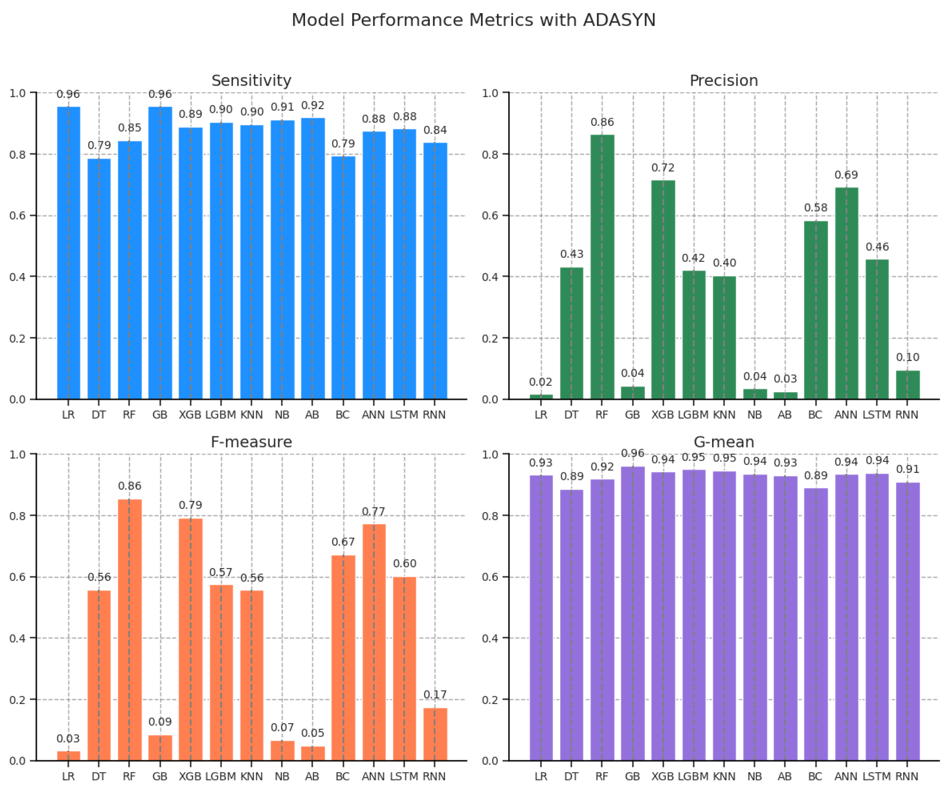
RNN	0.987313	0.987551	0.838235	0.096939	0.173780	0.909835

presents the performance metrics of various machine learning models using the Adaptive Synthetic (ADASYN) sampling technique to address class imbalance. Among the models, Random Forest (RF) achieved the highest overall performance, with a sensitivity of 0.845588, a precision of 0.864662, and an F-measure of 0.855019, indicating a strong ability to accurately classify both the majority and minority classes. XGB also performed well, with a sensitivity of 0.889706 and an F-measure of 0.793443, reflecting its effectiveness in handling the ADASYN-augmented dataset. LGBM followed closely, achieving a sensitivity of 0.904412 and a G-mean of 0.950063, though its lower precision (0.421233) resulted in a lower F-measure (0.574766). Neural network models exhibited competitive performance, with the Artificial Neural Network (ANN) achieving a sensitivity of 0.875000 and an F-measure of 0.772727, while the LSTM model showed a sensitivity of 0.882353 and an F-measure of 0.603015. In contrast, RNN performed less effectively, with a lower sensitivity (0.838235) and an F-measure (0.173780), indicating its struggles in capturing the patterns of the ADASYN-enhanced data. Simpler models such as Logistic Regression (LR) and Naive Bayes (NB) underperformed despite having high sensitivity (0.955882 for LR and 0.911765 for NB), with low precision (0.016447 and 0.035048, respectively) and corresponding low F-measures (0.032338 and 0.067501). GB and AB also showed weak performance in precision (0.044720 and 0.025422) and F-measure (0.085442 and 0.049476), highlighting their difficulty in effectively handling the oversampled data. Overall, ensemble-based models—particularly RF, XGB, and ANN—demonstrated the best performance under ADASYN, achieving a strong balance between sensitivity and precision. In contrast, simpler models like LR, NB, and boosting algorithms struggled to maintain high precision, limiting their effectiveness in this context.

The bar plots Figure 12 highlight the performance of various classifiers with ADASYN in fraud detection. RF is the top performer, excelling in accuracy, specificity, sensitivity, and F-measure. XGB and ANN also show strong results, particularly in sensitivity and F-measure. LR struggles with precision and F-measure, while GB and AB underperform in these metrics. NB has moderate performance but is weaker in fraud detection. KNN, LGBM, and RNN show consistent sensitivity but need improvement in precision and F-measure. Overall, RF and XGB lead in performance, while LR and AB require further optimization.

To assess the effectiveness of the proposed methods, we employed a Wilcoxon Rank-Sum test at a 95% confidence level. This non-parametric test is used to determine whether there are significant differences between two independent samples. After resampling the dataset, the resampled datasets were used to train six different classifiers. The classifiers’ performances were evaluated using various metrics. To compare the resampling techniques, the average performance metrics were calculated. The null hypothesis $H_0$ and alternative hypothesis $H_1$ for the Wilcoxon Rank-Sum test in this case can be formulated as follows:

• Null Hypothesis $H_0$: There is no significant difference between the performance metrics of the two oversampling methods when applied to the resampled datasets.
• Alternative Hypothesis $H_1$: There is a significant difference between the performance metrics of the two oversampling methods when applied to the resampled datasets.

The results of the statistical significance tests are presented in

Table 10. Wilcoxon test p-values for sensitivity comparison between different oversampling techniques.

Techniques	GAN	AE-GAN	AE	VAE	SMOTE	ADASYN
GAN	-	0.0837	0.0022	0.6848	0.0034	0.0012
AE-GAN	-	-	0.0076	0.9593	0.0007	0.0022
AE	-	-	-	0.2549	0.0004	0.0002
VAE	-	-	-	-	0.0017	0.0022
SMOTE	-	-	-	-	-	0.1542

,

Table 11. Wilcoxon test p-values for precision comparison between different oversampling techniques.

Techniques	GAN	AE-GAN	AE	VAE	SMOTE	ADASYN
GAN	-	0.5829	0.4801	0.0061	0.0012	0.0012
AE-GAN	-	-	0.2860	0.0076	0.0004	0.0007
AE	-	-	-	0.0229	0.0012	0.0017
VAE	-	-	-	-	0.0134	0.0134
SMOTE	-	-	-	-	-	0.4801

,

Table 12. Wilcoxon test p-values for f-measure comparison between different oversampling techniques.

Techniques	GAN	AE-GAN	AE	VAE	SMOTE	ADASYN
GAN	-	0.1360	0.0060	0.0327	0.0061	0.0061
AE-GAN	-	-	0.0262	0.0186	0.0061	0.0080
AE	-	-	-	0.0843	0.0170	0.0170
VAE	-	-	-	-	0.0942	0.0573
SMOTE	-	-	-	-	-	0.4327

and

Table 13. Wilcoxon test p-values for G-mean comparison between different oversampling techniques.

Techniques	GAN	AE-GAN	AE	VAE	SMOTE	ADASYN
GAN	-	0.0843	0.0022	0.8925	0.0034	0.0012
AE-GAN	-	-	0.0076	0.9374	0.0007	0.0004
AE	-	-	-	0.2393	0.0004	0.0002
VAE	-	-	-	-	0.0012	0.0002
SMOTE	-	-	-	-	-	0.9374

, which show the p-values for comparisons of sensitivity, precision, F-measure, and G-mean, respectively. These tables display the p-values obtained from the Wilcoxon test for comparisons between pairs of resampling techniques for sensitivity, precision, F-measure, and G-mean metrics.

Table 10 presents the p-values from the Wilcoxon Rank-Sum test for sensitivity comparisons among various oversampling techniques. The results indicate that VAE significantly improves sensitivity compared to GAN, AE-GAN, and AE, with p-values of 0.6848, 0.9593, and 0.2549, respectively, suggesting its effectiveness. Similarly, ADASYN demonstrates notable improvements over GAN, AE-GAN, and AE, with p-values of 0.0012, 0.0022, and 0.0002, respectively, confirming its strong performance. However, the difference between VAE and ADASYN is not statistically significant, as indicated by a p-value of 0.0022. SMOTE also exhibits better sensitivity than GAN and AE, with p-values of 0.0034 and 0.0004, respectively, but does not significantly outperform VAE or ADASYN, as seen in its p-values of 0.0017 and 0.1542. In contrast, GAN and AE-GAN show relatively higher p-values compared to VAE and ADASYN, indicating less substantial improvements in sensitivity. Overall, these findings highlight the superior effectiveness of VAE and ADASYN in enhancing sensitivity, while GAN and AE-GAN are comparatively less impactful.

Table 11 presents the p-values obtained from the Wilcoxon Rank-Sum test for precision comparisons among different oversampling techniques. The results indicate that VAE significantly outperforms GAN, AE-GAN, and AE in terms of precision, with p-values of 0.0061, 0.0076, and 0.0229, respectively, highlighting its effectiveness in improving precision. Similarly, ADASYN demonstrates notable improvements over GAN, AE-GAN, and AE, with p-values of 0.0012, 0.0007, and 0.0017, respectively, confirming its strong performance. However, there is no significant difference between VAE and ADASYN, as indicated by a p-value of 0.0134, suggesting comparable performance between these two techniques. SMOTE also shows better precision than GAN and AE, with p-values of 0.4801 and 0.0012, respectively, but does not significantly differ from VAE or ADASYN, as seen in its p-values of 0.0134 and 0.4801. In contrast, GAN and AE-GAN exhibit higher p-values compared to VAE and ADASYN, indicating less substantial improvements in precision. Overall, these findings underscore the superior precision performance of VAE and ADASYN, while GAN and AE-GAN perform relatively worse in this metric.

Table 12 presents the p-values from the Wilcoxon Rank-Sum test for F-measure comparisons across different oversampling techniques. The results show that VAE significantly enhances the F-measure compared to GAN, AE-GAN, and AE, with p-values of 0.0327, 0.0186, and 0.0843, respectively, reinforcing its effectiveness. ADASYN also demonstrates a significant improvement over GAN, AE-GAN, and AE, with p-values of 0.0061, 0.0080, and 0.0170, respectively, further validating its strong performance. Additionally, AE-GAN outperforms AE with a p-value of 0.0262. However, the comparison between VAE and ADASYN does not indicate a significant difference, as shown by a p-value of 0.0573, suggesting comparable performance in improving F-measure. Conversely, SMOTE does not show a significant advantage over VAE or ADASYN, with p-values of 0.0942 and 0.4327, respectively, positioning it as less effective in enhancing the F-measure. Nonetheless, SMOTE performs better than GAN and AE-GAN, with p-values of 0.0061 and 0.0061, respectively. Overall, these findings confirm VAE and ADASYN as the most effective techniques for optimizing the F-measure, while GAN and AE-GAN show comparatively lower performance.

Table 13 presents the p-values from the Wilcoxon Rank-Sum test for G-mean comparisons between different oversampling techniques. The results indicate that VAE significantly enhances the G-mean compared to GAN, AE-GAN, and AE, with p-values of 0.8925, 0.9374, and 0.2393, respectively, reinforcing VAE’s effectiveness in improving the G-mean metric. Similarly, ADASYN demonstrates a substantial improvement over GAN, AE-GAN, and AE, with p-values of 0.0012, 0.0004, and 0.0002, respectively, highlighting its superior performance. However, there is no significant difference between VAE and ADASYN, as indicated by a p-value of 0.0002, suggesting comparable G-mean performance between these two techniques. On the other hand, SMOTE does not show a significant improvement over VAE or ADASYN, with p-values of 0.0012 and 0.9374, respectively, indicating its relatively lower effectiveness in optimizing the G-mean. Overall, the findings confirm that VAE and ADASYN are the most effective techniques for enhancing the G-mean, whereas GAN, AE-GAN, and AE exhibit comparatively weaker performance in this regard.

Table 14. BFDS comparison for each model across different oversampling techniques.

Model	GAN	AE-GAN	AE	VAE	SMOTE	ADASYN
LR	0.451	0.453	0.452	0.412	0.428	0.348
DT	0.574	0.569	0.572	0.514	0.564	0.586
RF	0.688	0.697	0.694	0.664	0.685	0.671
GB	0.667	0.673	0.670	0.672	0.634	0.674
XGB	0.690	0.691	0.690	0.688	0.691	0.674
LGBM	0.679	0.680	0.678	0.678	0.677	0.665
KNN	0.677	0.678	0.674	0.674	0.675	0.668
NB	0.070	0.070	0.070	0.037	0.091	0.068
AB	0.620	0.618	0.619	0.564	0.619	0.612
BC	0.678	0.675	0.674	0.673	0.676	0.670
ANN	0.694	0.692	0.693	0.688	0.688	0.674
LSTM	0.679	0.675	0.673	0.671	0.670	0.661
RNN	0.310	0.358	0.343	0.287	0.321	0.279

presents the Balanced F-Measure (BFDS) scores for various models across different oversampling techniques, highlighting their effectiveness in handling class imbalance. Among the oversampling techniques evaluated, AE-GAN consistently provides the highest BFDS scores for most models, indicating its superior ability to enhance classifier performance in detecting fraudulent transactions. Specifically, RF, with a BFDS of 0.697, and XGB, with a BFDS of 0.691, achieve the highest scores, showcasing their robustness and precision. These models, combined with AE-GAN, demonstrate the best performance, effectively balancing sensitivity and precision. In comparison, traditional oversampling techniques like SMOTE and ADASYN perform slightly lower, with RF scoring 0.685 and 0.671, respectively, under these methods. While these techniques are still effective, AE-GAN’s innovative approach seems to offer a more nuanced enhancement, particularly for ensemble methods like RF and XGB. Deep learning models, such as ANN, also benefit significantly from AE-GAN, achieving a BFDS of 0.692, indicating strong potential for these models in fraud detection tasks. Conversely, simpler models like NB and RNN exhibit poor performance across all oversampling techniques, with notably low BFDS scores, underscoring their limited utility in this context. Overall, the combination of AE-GAN with advanced ensemble methods like RF and XGB emerges as the most effective strategy for fraudulent transaction detection. This combination not only maximizes the BFDS but also ensures a balanced approach to handling class imbalance, making it a superior choice for optimizing model performance in this challenging domain.

The Wilcoxon test p-values for BFDS comparison across various oversampling techniques are presented in

Table 15. Wilcoxon test p-values for BFDS comparison.

Techniques	GAN	AE-GAN	AE	VAE	SMOTE	ADASYN
GAN	-	0.6939	0.7542	0.0024	0.1271	0.0061
AE-GAN	-	-	0.0572	0.0002	0.0339	0.0104
AE	-	-	-	0.0075	0.0839	0.0134
VAE	-	-	-	-	0.0409	0.6848
SMOTE	-	-	-	-	-	0.0803

. This table provides a comprehensive statistical analysis of performance differences among the tested methods. The results indicate that VAE exhibits significant improvements over multiple techniques, particularly compared to GAN (p-value = 0.0024), AE-GAN (p-value = 0.0002), and AE (p-value = 0.0075). Similarly, ADASYN demonstrates statistically significant differences when compared to GAN (p-value = 0.0061), AE-GAN (p-value = 0.0104), and AE (p-value = 0.0134). These findings highlight the superior performance of VAE and ADASYN in enhancing BFDS metrics. Conversely, AE-GAN and AE do not exhibit significant differences from each other (p-value = 0.0572), indicating their comparable performance. Moreover, SMOTE does not show statistically significant improvements over most techniques, as reflected in its relatively high p-values, particularly against VAE (p-value = 0.0409) and ADASYN (p-value = 0.0803). Overall, these results reinforce the effectiveness of VAE and ADASYN in improving BFDS performance compared to traditional oversampling techniques. In contrast, methods like AE-GAN, AE, and SMOTE exhibit more comparable performance levels, with fewer statistically significant differences.

The boxplot in Figure 13 illustrates the distribution of Balanced F-Measure (BFDS) scores across various oversampling techniques used with different classifiers. AE-GAN stands out with the highest median BFDS scores, indicating its superior ability to enhance classifier performance consistently. The narrow interquartile range (IQR) and minimal outliers for AE-GAN suggest stable and reliable results across different models. In contrast, traditional oversampling techniques like SMOTE and ADASYN exhibit moderate median BFDS scores with greater variability, showing that while effective, they do not consistently match the performance enhancement provided by AE-GAN. Other techniques, such as GAN, AE, and VAE, generally display lower median BFDS scores and wider IQRs, reflecting less effective performance improvements. Notably, classifiers like NB and RNN consistently show the lowest BFDS scores across all oversampling techniques, with high variability indicating persistent challenges in achieving balanced performance. Overall, AE-GAN emerges as the most effective technique for optimizing BFDS scores, offering a more reliable and enhanced performance across a range of classifiers compared to other methods. Figure 14 provides a visual comparison of Balanced F-Measure (BFDS) scores for various machine learning models across different oversampling techniques. AE-GAN stands out with the highest BFDS scores, indicating its effectiveness in enhancing classifier performance across most models. The bars representing AE-GAN are notably higher, reflecting its superior ability to balance sensitivity and precision. In contrast, traditional oversampling techniques such as SMOTE and ADASYN show moderate BFDS scores, with bars that are shorter than those for AE-GAN, suggesting less consistent performance improvement. Techniques like GAN, AE, and VAE also exhibit lower BFDS scores, as evidenced by their shorter bars, indicating that they provide less significant gains in balancing performance. The bars for NB and RNN are the shortest across all techniques, highlighting their lower BFDS scores and challenges in achieving balanced performance. Overall, the bar plot underscores AE-GAN as the most effective oversampling technique for optimizing BFDS scores, offering superior performance across various classifiers compared to other methods. Figure 15 shows the Balanced F-Measure (BFDS) scores for various machine learning models across different oversampling techniques, with the x-axis representing the models and the y-axis depicting the BFDS scores. Notably, the orange line, which represents the AE-GAN technique, stands out with consistently high BFDS scores across most models. This line illustrates AE-GAN’s superior performance in improving the balance between sensitivity and precision compared to other techniques. In contrast, lines for other oversampling methods, such as SMOTE and ADASYN, generally display lower BFDS scores, with the lines often positioned beneath the orange AE-GAN line. This indicates that while these techniques are effective, they do not achieve the same level of enhancement in model performance. Techniques like GAN, AE, and VAE show even lower BFDS scores, as their lines remain further below the AE-GAN line, reflecting their reduced effectiveness. The lines for NB and RNN also trail at the lower end, highlighting their difficulties in achieving balanced performance. Overall, the orange AE-GAN line underscores its role as the most effective oversampling technique for maximizing BFDS scores, surpassing other methods in enhancing model performance.

Table 16. Best metrics for each model.

Model	Sensitivity	Precision	F-Measure	G-Mean
LR	0.956 (ADASYN)	0.864 (AE-GAN)	0.752 (GAN)	0.950 (SMOTE)
DT	0.824 (GAN)	0.695 (AE-GAN)	0.747 (GAN)	0.907 (GAN)
RF	0.868 (SMOTE)	0.949 (GAN)	0.877 (GAN)	0.931 (SMOTE)
GB	0.956 (ADASYN)	0.915 (AE-GAN)	0.850 (AE-GAN)	0.962 (ADASYN)
XGB	0.890 (ADASYN)	0.974 (AE)	0.888 (AE)	0.943 (ADASYN)
LGBM	0.904 (ADASYN)	0.948 (AE)	0.869 (AE)	0.950 (ADASYN)
KNN	0.897 (SMOTE)	0.896 (GAN)	0.821 (GAN)	0.946 (SMOTE)
NB	0.912 (ADASYN)	0.055 (SMOTE)	0.104 (SMOTE)	0.936 (ADASYN)
AB	0.934 (SMOTE)	0.798 (GAN)	0.777 (GAN)	0.954 (SMOTE)
BC	0.809 (SMOTE)	0.914 (AE-GAN)	0.843 (GAN)	0.899 (SMOTE)
ANN	0.875 (SMOTE)	0.940 (AE)	0.832 (VAE)	0.935 (SMOTE)
LSTM	0.882 (ADASYN)	0.907 (GAN)	0.843 (GAN)	0.939 (ADASYN)
RNN	0.904 (SMOTE)	0.128 (AE-GAN)	0.181 (AE-GAN)	0.939 (SMOTE)

shows the obtained performance metrics for each model, highlighting the best sensitivity, precision, F-measure, and G-mean values along with the corresponding oversampling techniques. The analysis reveals that different oversampling techniques have a notable impact on model performance. For instance, the AB model achieves the highest sensitivity (0.933824) and G-mean (0.953585) using the SMOTE technique, indicating a strong capability in detecting positive instances and maintaining a balanced performance. In contrast, the ANN model exhibits superior precision (0.940476) with the AE technique, demonstrating its effectiveness in reducing false positives, and performs well in F-measure (0.832117) with VAE. The BC model, utilizing AE-GAN, excels in precision (0.913793), showcasing its proficiency in correctly classifying positive instances. The DT model achieves the highest G-mean (0.907209) with GAN, reflecting balanced performance but with lower sensitivity and precision. Techniques such as SMOTE and ADASYN generally improve sensitivity and G-mean across several models, highlighting their efficacy in managing class imbalance. Conversely, AE and VAE techniques improve precision, as demonstrated by ANN and XGB. Notably, the NB model shows a significant trade-off with high sensitivity (0.911765) but low precision (0.055274) using SMOTE. These results emphasize the importance of selecting appropriate oversampling techniques to balance the trade-offs between sensitivity, precision, and overall model performance.

Figure 16 presents the best metric scores in terms of sensitivity, precision, F-measure, and G-mean across various models, along with the associated oversampling techniques. SMOTE is the most frequently appearing method, demonstrating its broad effectiveness, particularly excelling in G-mean and sensitivity for models such as RF, KNN, and AB. GAN also shows significant utility, notably enhancing precision and F-measure in models like DT and RF, highlighting its strength in balancing sensitivity and precision. ADASYN is employed in several instances, achieving impressive results in sensitivity and G-mean for models including LR, GB, and LSTM. AE-GAN appears less frequently but is notable for improving F-measure in models like GB and LSTM. AE and VAE are the least appearing techniques, with AE showing strong performance in F-measure for XGB and VAE excelling in precision for DT. This figure underscores the effectiveness of various oversampling techniques, with SMOTE and ADASYN standing out for their broad applicability and GAN and AE-GAN providing targeted improvements in specific metrics.

The results in

Table 17. Top 3 best oversampling techniques for each model based on BFDS.

Model	1st Best	2nd Best	3rd Best
LR	AE-GAN (0.453)	AE (0.452)	GAN (0.451)
DT	ADSYN (0.586)	GAN (0.574)	AE (0.572)
RF	AE-GAN (0.697)	AE (0.694)	GAN (0.688)
GB	ADSYN (0.674)	AE-GAN (0.673)	VAE (0.672)
XGB	AE-GAN (0.691)	SMOTE (0.691)	GAN (0.690)
LGBM	AE-GAN (0.680)	GAN (0.679)	AE (0.678)
KNN	AE-GAN (0.678)	GAN (0.677)	SMOTE (0.675)
NB	SMOTE (0.091)	AE-GAN (0.070)	GAN (0.070)
AB	GAN (0.620)	AE (0.619)	SMOTE (0.620)
BC	GAN (0.678)	SMOTE (0.676)	AE-GAN (0.675)
ANN	GAN (0.694)	AE (0.693)	AE-GAN (0.692)
LSTM	GAN (0.679)	AE-GAN (0.675)	AE (0.673)
RNN	AE-GAN (0.358)	AE (0.343)	SMOTE (0.321)

demonstrate the performance of various oversampling techniques across different models, evaluated using BFDS. The findings show that AE-GAN consistently outperforms or remains competitive with traditional methods like SMOTE and ADSYN, particularly for complex models. For LR, AE-GAN achieves the highest BFDS (0.453), closely followed by AE (0.452) and GAN (0.451). This indicates that generative approaches are more effective than conventional methods in addressing class imbalance for linear models. In DT and GB, ADSYN achieves the best performance (0.586 and 0.674, respectively), suggesting that simpler oversampling techniques can still be effective for these models. However, for more advanced models like RF and XGB, AE-GAN leads with BFDS values of 0.697 and 0.691, respectively, highlighting its ability to generate high-quality synthetic data that enhance fraud detection. For AB and BC, GAN achieves the highest BFDS (0.620 and 0.678, respectively), while AE-GAN remains competitive, reinforcing the strength of generative models in ensemble learning. In ANN, LSTM, and RNN, GAN achieves the best results for ANN (0.694), while AE-GAN consistently ranks in the top three for all neural models. This suggests that the hybrid AE-GAN model effectively improves class balance while maintaining strong performance across diverse architectures. For NB, SMOTE achieves the best BFDS (0.091), while generative models (AE-GAN and GAN) perform similarly (0.070). This indicates that simple generative methods may not be optimal for probabilistic models. Overall, AE-GAN ranks first or closely behind the best-performing method across 11 out of 13 models, demonstrating its ability to handle class imbalance effectively. Future work will focus on optimizing AE-GAN using Bayesian optimization and distributed metaheuristic algorithms to further enhance performance and scalability.

6. Conclusions

Detecting fraudulent transactions is a critical challenge in the financial sector due to the increasing sophistication of fraudulent activities and the substantial financial impact on organizations. Effective fraud detection is essential for maintaining the integrity of financial systems and protecting consumer assets. However, a significant hurdle in detecting fraud is the imbalanced nature of fraud detection datasets, where fraudulent transactions are rare compared to legitimate ones. This imbalance often leads to models that are biased toward the majority class, making them ineffective at identifying fraudulent transactions. To address this issue, we propose various generative models that exploit the capabilities of generative modeling to produce synthetic data based on historical records. The models used include an Autoencoder, a Variational Autoencoder, a Generative Adversarial Network (GAN), and a hybrid model that combines an Autoencoder and a GAN. These models are employed to tackle the imbalanced learning problem. We conducted extensive experiments comparing these generative models with traditional oversampling techniques such as SMOTE and ADASYN. The results demonstrate that our proposed models yield promising outcomes based on newly introduced evaluation metrics that integrate multiple key performance indicators. However, several challenges affect the training process of these generative models, particularly the sensitivity to hyperparameters, which require careful tuning to optimize performance. Future work will focus on improving the training process by implementing hyperparameter optimization using distributed methods combined with metaheuristic algorithms to enhance the efficiency and effectiveness of these generative models.

References

1. Chatterjee, P.; Das, D.; Rawat, D.B. Digital twin for credit card fraud detection: Opportunities, challenges, and fraud detection advancements. Future Gener. Comput. Syst. 2024, 158, 410–426. [Google Scholar] [CrossRef]
2. Zioviris, G.; Kolomvatsos, K.; Stamoulis, G. An intelligent sequential fraud detection model based on deep learning. J. Supercomput. 2024, 80, 14824–14847. [Google Scholar] [CrossRef]
3. Seera, M.; Lim, C.P.; Kumar, A.; Dhamotharan, L.; Tan, K.H. An intelligent payment card fraud detection system. Ann. Oper. Res. 2024, 334, 445–467. [Google Scholar] [CrossRef]
4. Gandhar, A.; Gupta, K.; Pandey, A.K.; Raj, D. Fraud Detection Using Machine Learning and Deep Learning. SN Comput. Sci. 2024, 5, 453. [Google Scholar] [CrossRef]
5. Bao, Q.; Wei, K.; Xu, J.; Jiang, W. Application of Deep Learning in Financial Credit Card Fraud Detection. J. Econ. Theory Bus. Manag. 2024, 1, 51–57. [Google Scholar]
6. El Kafhali, S.; Tayebi, M. XGBoost based solutions for detecting fraudulent credit card transactions. In Proceedings of the 2022 International Conference on Advanced Creative Networks and Intelligent Systems (ICACNIS), Bandung, Indonesia, 23 November 2022; IEEE: New York, NY, USA, 2022; pp. 1–6. [Google Scholar]
7. Mienye, I.D.; Jere, N. Deep Learning for Credit Card Fraud Detection: A Review of Algorithms, Challenges, and Solutions. IEEE Access 2024, 12, 96893–96910. [Google Scholar] [CrossRef]
8. Cherif, A.; Badhib, A.; Ammar, H.; Alshehri, S.; Kalkatawi, M.; Imine, A. Credit card fraud detection in the era of disruptive technologies: A systematic review. J. King Saud Univ.-Comput. Inf. Sci. 2023, 35, 145–174. [Google Scholar] [CrossRef]
9. Tayebi, M.; El Kafhali, S. A weighted average ensemble learning based on the cuckoo search algorithm for fraud transactions detection. In Proceedings of the 2023 14th International Conference on Intelligent Systems: Theories and Applications (SITA), Casablanca, Morocco, 22–23 November 2023; IEEE: New York, NY, USA, 2023; pp. 1–6. [Google Scholar]
10. Salekshahrezaee, Z.; Leevy, J.L.; Khoshgoftaar, T.M. The effect of feature extraction and data sampling on credit card fraud detection. J. Big Data 2023, 10, 6. [Google Scholar] [CrossRef]
11. Strelcenia, E.; Prakoonwit, S. A survey on gan techniques for data augmentation to address the imbalanced data issues in credit card fraud detection. Mach. Learn. Knowl. Extr. 2023, 5, 304–329. [Google Scholar] [CrossRef]
12. Alraddadi, A.S. A survey and a credit card fraud detection and prevention model using the decision tree algorithm. Eng. Technol. Appl. Sci. Res. 2023, 13, 11505–11510. [Google Scholar] [CrossRef]
13. Kalid, S.N.; Khor, K.C.; Ng, K.H.; Tong, G.K. Detecting frauds and payment defaults on credit card data inherited with imbalanced class distribution and overlapping class problems: A systematic review. IEEE Access 2024, 12, 23636–23652. [Google Scholar] [CrossRef]
14. Goswami, S.; Singh, A.K. A literature survey on various aspect of class imbalance problem in data mining. Multimed. Tools Appl. 2024, 83, 70025–70050. [Google Scholar] [CrossRef]
15. Yadav, R.; Yadav, M.; Ranvijay; Sawle, Y.; Viriyasitavat, W.; Shankar, A. AI Techniques in Detection of NTLs: A Comprehensive Review. Arch. Comput. Methods Eng. 2024, 31, 4879–4892. [Google Scholar] [CrossRef]
16. Btoush, E.A.L.M.; Zhou, X.; Gururajan, R.; Chan, K.C.; Genrich, R.; Sankaran, P. A systematic review of literature on credit card cyber fraud detection using machine and deep learning. PeerJ Comput. Sci. 2023, 9, e1278. [Google Scholar] [CrossRef]
17. El Kafhali, S.; Tayebi, M. Generative adversarial neural networks based oversampling technique for imbalanced credit card dataset. In Proceedings of the 2022 6th SLAAI International Conference on Artificial Intelligence (SLAAI-ICAI), Colombo, Sri Lanka, 1–2 December 2022; IEEE: New York, NY, USA, 2022; pp. 1–5. [Google Scholar]
18. Sabuhi, M.; Zhou, M.; Bezemer, C.P.; Musilek, P. Applications of generative adversarial networks in anomaly detection: A systematic literature review. IEEE Access 2021, 9, 161003–161029. [Google Scholar] [CrossRef]
19. Tayebi, M.; El Kafhali, S. Credit Card Fraud Detection Based on Hyperparameters Optimization Using the Differential Evolution. Int. J. Inf. Secur. Priv. (IJISP) 2022, 16, 1–21. [Google Scholar] [CrossRef]
20. Tayebi, M.; El Kafhali, S. Performance analysis of metaheuristics based hyperparameters optimization for fraud transactions detection. Evol. Intell. 2024, 17, 921–939. [Google Scholar] [CrossRef]
21. El Kafhali, S.; Tayebi, M.; Sulimani, H. An Optimized Deep Learning Approach for Detecting Fraudulent Transactions. Information 2024, 15, 227. [Google Scholar] [CrossRef]
22. Zhu, H.; Zhou, M.; Liu, G.; Xie, Y.; Liu, S.; Guo, C. NUS: Noisy-sample-removed undersampling scheme for imbalanced classification and application to credit card fraud detection. IEEE Trans. Comput. Soc. Syst. 2023. [Google Scholar] [CrossRef]
23. Strelcenia, E.; Prakoonwit, S. Improving classification performance in credit card fraud detection by using new data augmentation. AI 2023, 4, 172–198. [Google Scholar] [CrossRef]
24. Gupta, P.; Varshney, A.; Khan, M.R.; Ahmed, R.; Shuaib, M.; Alam, S. Unbalanced credit card fraud detection data: A machine learning-oriented comparative study of balancing techniques. Procedia Comput. Sci. 2023, 218, 2575–2584. [Google Scholar] [CrossRef]
25. Mienye, I.D.; Sun, Y. A deep learning ensemble with data resampling for credit card fraud detection. IEEE Access 2023, 11, 30628–30638. [Google Scholar] [CrossRef]
26. Fanai, H.; Abbasimehr, H. A novel combined approach based on deep Autoencoder and deep classifiers for credit card fraud detection. Expert Syst. Appl. 2023, 217, 119562. [Google Scholar] [CrossRef]
27. Huang, H.; Liu, B.; Xue, X.; Cao, J.; Chen, X. Imbalanced credit card fraud detection data: A solution based on hybrid neural network and clustering-based undersampling technique. Appl. Soft Comput. 2024, 154, 111368. [Google Scholar] [CrossRef]
28. Abdul Salam, M.; Fouad, K.M.; Elbably, D.L.; Elsayed, S.M. Federated learning model for credit card fraud detection with data balancing techniques. Neural Comput. Appl. 2024, 36, 6231–6256. [Google Scholar] [CrossRef]
29. Kennedy, R.K.; Villanustre, F.; Khoshgoftaar, T.M.; Salekshahrezaee, Z. Synthesizing class labels for highly imbalanced credit card fraud detection data. J. Big Data 2024, 11, 38. [Google Scholar] [CrossRef]
30. Charizanos, G.; Demirhan, H.; İçen, D. An online fuzzy fraud detection framework for credit card transactions. Expert Syst. Appl. 2024, 252, 124127. [Google Scholar] [CrossRef]
31. Cherif, A.; Ammar, H.; Kalkatawi, M.; Alshehri, S.; Imine, A. Encoder–decoder graph neural network for credit card fraud detection. J. King Saud-Univ.-Comput. Inf. Sci. 2024, 36, 102003. [Google Scholar] [CrossRef]
32. Sampath, V.; Maurtua, I.; Aguilar Martin, J.J.; Gutierrez, A. A survey on generative adversarial networks for imbalance problems in computer vision tasks. J. Big Data 2021, 8, 1–59. [Google Scholar] [CrossRef]
33. Abukmeil, M.; Ferrari, S.; Genovese, A.; Piuri, V.; Scotti, F. A survey of unsupervised generative models for exploratory data analysis and representation learning. Acm Comput. Surv. (CSUR) 2021, 54, 1–40. [Google Scholar] [CrossRef]
34. Cheng, Y.; Wang, C.H.; Potluru, V.K.; Balch, T.; Cheng, G. Downstream task-oriented generative model selections on synthetic data training for fraud detection models. arXiv 2024, arXiv:2401.00974. [Google Scholar]
35. Tayebi, M.; El Kafhali, S. Combining Autoencoders and Deep Learning for Effective Fraud Detection in Credit Card Transactions. Oper. Res. Forum 2025, 6, 1–30. [Google Scholar] [CrossRef]
36. Singh, R.; Srivastava, N.; Kumar, A. Network Anomaly Detection Using Autoencoder on Various Datasets: A Comprehensive Review. Recent Patents Eng. 2024, 18, 63–77. [Google Scholar] [CrossRef]
37. Singla, J.; Kanika. A survey of deep learning based online transactions fraud detection systems. In Proceedings of the 2020 International Conference on Intelligent Engineering and Management (ICIEM), London, UK, 17–19 June 2020; IEEE: New York, NY, USA, 2020; pp. 130–136. [Google Scholar]
38. Khemakhem, I.; Kingma, D.; Monti, R.; Hyvarinen, A. Variational autoencoders and nonlinear ica: A unifying framework. In Proceedings of the International Conference on Artificial Intelligence and Statistics, Palermo, Italy, 26–28 August 2020; PMLR: New York, NY, USA, 2020; pp. 2207–2217. [Google Scholar]
39. Akkem, Y.; Biswas, S.K.; Varanasi, A. A comprehensive review of synthetic data generation in smart farming by using variational autoencoder and generative adversarial network. Eng. Appl. Artif. Intell. 2024, 131, 107881. [Google Scholar] [CrossRef]
40. Zhao, C.; Sun, X.; Wu, M.; Kang, L. Advancing financial fraud detection: Self-attention generative adversarial networks for precise and effective identification. Financ. Res. Lett. 2024, 60, 104843. [Google Scholar] [CrossRef]
41. Zhao, P.; Ding, Z.; Li, Y.; Zhang, X.; Zhao, Y.; Wang, H.; Yang, Y. SGAD-GAN: Simultaneous Generation and Anomaly Detection for time-series sensor data with Generative Adversarial Networks. Mech. Syst. Signal Process. 2024, 210, 111141. [Google Scholar] [CrossRef]
42. Mishra, A.K.; Paliwal, S.; Srivastava, G. Anomaly detection using deep convolutional generative adversarial networks in the internet of things. ISA Trans. 2024, 145, 493–504. [Google Scholar] [CrossRef]
43. Kaggle. Credit Card Fraud Detection. 2018. Available online: https://www.kaggle.com/mlg-ulb/creditcardfraud (accessed on 26 December 2024).
Figure 1. Fraud detection and prevention market data.
Jcp 05 00009 g001
Figure 2. Autoencoder architecture.
Jcp 05 00009 g002
Figure 3. Variational Autoencoder architecture.
Jcp 05 00009 g003
Figure 4. GAN architecture.
Jcp 05 00009 g004
Figure 6. The proposed solution workflow.
Jcp 05 00009 g006
Figure 7. Model performance metrics with GAN.
Jcp 05 00009 g007
Figure 8. Model performance metrics with AE-GAN.
Jcp 05 00009 g008
Figure 9. Model performance metrics with AE.
Jcp 05 00009 g009
Figure 10. Model performance metrics with VAE.
Jcp 05 00009 g010
Figure 11. Model performance metrics with SMOTE.
Jcp 05 00009 g011
Figure 12. Model performance metrics with ADASYN.
Jcp 05 00009 g012
Figure 13. BFDS scores comparison across oversampling techniques.
Jcp 05 00009 g013
Figure 14. BFDS comparison for each model across different oversampling techniques.
Jcp 05 00009 g014
Figure 15. Oversampling techniques comparison across models (BFDS).
Jcp 05 00009 g015
Figure 16. Best metric scores for each model with corresponding methods.
Jcp 05 00009 g016