Machine Learning-Based Attack Detection and Mitigation with Multi-Controller Placement Optimization over SDN Environment

Abstract

The increasing complexity and scale of modern software-defined networking demands advanced solutions to address security challenges, particularly distributed denial-of-service (DDoS) attacks in multi-controller environments. Traditional single-controller implementations are struggling to effectively counter sophisticated cyber threats, necessitating a faster and scalable solution. This study introduces a novel approach for attack detection and mitigation with optimized multi-controller software-defined networking (SDN) using machine learning (ML). The study focuses on the design, implementation, and assessment of the optimal placement of multi-controllers using K-means++ and OPTICS in real topologies and an intrusion detection system (IDS) using the XGBoost classification algorithm to detect and mitigate attacks efficiently with accuracy, precision, and recall of 98.5%, 97.0%, and 97.0%, respectively. Additionally, the IDS decouples from the controllers, preserves controller resources, and allows for efficient near-real-time attack detection and mitigation. The proposed solution outperforms well by autonomously identifying anomalous behaviors in networks through successfully combining the controller placement problem (CPP) and DDoS security.

1. Introduction

Software-defined networking (SDN) is a newer network paradigm consisting of three planes, viz. data, control, and application planes, where data and control planes are independent of one another [1]. In traditional network architecture, the control plane and data plane are interconnected [2,3]. SDN is a cutting-edge paradigm that solves issues with traditional Internet architectures. It provides flexibility in management by allowing networking to be programmed from a logically centralized control point [4]. The controller uses a northbound Application Programming Interface (API) to communicate with the application layer and a southbound API to communicate with the data plane. An OpenFlow protocol is used for controller–switch communication. Because the control plane and the data plane are separated, SDN offers numerous benefits over traditional networks, including programmability, flexibility, and scalability. But this has also given rise to other SDN-specific security problems [5].

Although SDN architecture has many advantages compared with traditional networks, it is often subjected to network threats and attacks. These days, the security risks associated with SDN architecture are on par with those of conventional networks. SDN has to deal with novel security issues, particularly in terms of protecting the SDN architecture. As SDN adoption progresses, more security concerns are expected to arise [6].

Yang et al. [7] claim that future studies will focus on identifying Distributed Denial-of-Service (DDoS) attacks in topologies that link or communicate amongst several controllers. Implementing a solution that tackles this security concern is therefore essential. Machine learning (ML) algorithms for DDoS detection and mitigation have gained more attention because traditional methods are insufficient.

This study examines the feasibility and efficacy of using different ML algorithms, including Naive Bayes classifier, XGBoost, K-nearest neighbors (KNNs), random forest, neural network, and long short-term memory (LSTM), to identify DDoS attacks and mitigate in the data plane of SDN architecture. In our experiment, XGBoost offered both an optimum balance of test accuracy and test time, and it was therefore used to build an intrusion detection system (IDS) for detecting DDoS attacks in SDN architecture. The main contributions of this paper are summarized as follows:

• Deployment of K-means++ and alternate density-based ordering points to identify the clustering structure (OPTICS) algorithms to determine the optimal number and optimal placement of multi-controllers.
• Development of novel algorithms for multi-controller SDN DDoS threat detection and resolution.
• Implementation of DDoS attack detection mechanism in the application plane and mitigation mechanism in the data plane.

The rest of the paper is organized as follows: The background and related work are discussed in Section 2. It includes SDN with multi-controllers and SDN security threats. Section 3 presents the detailed methodology. In Section 4, the results and discussion are presented. Here, we discuss optimal multi-controller placement algorithms, the system design scenario and performance evaluation of ML models. Finally, the conclusion and future work are presented in Section 5.

2. Background and the Related Work

2.1. SDN Security Threats and Attacks

SDN is becoming more challenging as a result of the significant rise in internet users and the resulting increase in network security risks. One of the most common and hazardous types of attacks in SDNs is DDoS [7,8]. Depending on the target plane, DDoS attacks in SDN can also be divided into three categories: application-layer, control-layer, and data-layer threats [9]. A number of strategies are employed for the detection, prevention, and mitigation of DDoS attacks, particularly on controllers in the SDN [10].

While SDN offers numerous benefits over cloud and network service providers (e.g., 5G/Telco/ISP), its widespread adoption is contingent upon addressing its security challenges. Targeted attacks have the ability to interfere with all three layers, primarily on the SDN software controller, making it the weakest link in the system overall, on the link between controllers (C2C), on the link between the controller and the switches (C2S), on the switches themselves, on applications, and on the link between the applications and the controller [5].

DDoS attack has the ability to completely destroy the network in addition to preventing unauthorized users from accessing and using network resources [11]. Consequently, defending the SDN network against DDoS attacks is essential.

There are different kinds of DDoS attacks, including ICMP flood, TCP flood, and UDP flood [12]. By running the attack source, an attacker drastically decreases the available bandwidth and stops the target host from communicating with the outside world by sending a lot of trash traffic to the target network.

Singh et al. [13] comprehensively reviewed about 70 well-known DDoS detection and mitigation techniques over SDN. Information theory-based approaches, machine learning-based methods, artificial neural networks (ANN)-based methods, and other miscellaneous methods are the four groups into which these techniques are classified. All the currently available DDoS detection solutions are divided into four groups based on the type of detection metric and detection technique used: information theory metrics, machine learning, artificial neural networks, and other defense solutions [9].

ML has become a popular tool for helping with threat and security analysis, intrusion detection, and other related tasks. Deeper insights can be gained by correctly examining ML’s support for a range of datasets produced by network traffic and a number of data characteristics [14].

Tahirou et al. [10] applied supervised ML methods, for example, Naive Bayes, support vector machine (SVM), and KNN for identifying DDoS attacks. The CIC-2019 dataset was used to train these algorithms. Ultimately, a real-time SDN simulation environment consisting of Mininet, Ryu controller, and SNORT NIDS was used to evaluate the performance of these approaches. As soon as an attack is detected and put to a blacklist for mitigation, the attacker’s IP address and port number are blocked.

SVM, hidden Markov model (HMM), decision tree (J48), Naive Bayes, the advanced support vector machine (ASVM), logistic regression, random trees, binary the bat algorithm, random forest, and KNN are some of the effective machine learning algorithms that many researchers have used for DDoS attack detection. Also, many researchers use effective algorithms, such as self-organizing maps (SOMs), exact-STORM, back-propagation neural nentwork (BPNN), convolution neural network (CNN), recurrent neural network (RNN), and LSTM, to identify DDoS attacks in SDN [9,15,16,17,18,19].

Meti et al. [20] used the NN classifier and the SVM classifier to identify the potentially hazardous connections. Mohsin et al. [21] examined the detection of DDoS attacks using four ML techniques: random forest, K-nearest neighbors, Naive Bayes, and logistic regression.

2.2. SDN with Multi-Controllers

Zhang et al. [22] explain that SDN offers flexibility in network configuration by separating the control plane from the data plane. Despite this potential, one of SDN’s drawbacks is that the controller reduces the overall availability of the network since it is a single point of failure. Multi-controller designs have been proposed as a way to offset the limitations of having a single controller in a network. Multiple controllers increase network reliability because they allow the data plane to keep running even in the event that one controller fails. For large networks, multi-controller implementation can solve the scalability and reliability issues introduced by the SDN centralized logical control concept.

Unlike single-controller SDN, multi-controller SDN introduces new challenges that directly impact security and network performance. Attackers employ correlated and distributed attacks, where they target only a subset of controllers before launching a coordinated attack on the entire network, which does not apply to single controller setups. Additionally, in a multi-controller system, each controller only has partial knowledge of the overall network state. This means security mechanisms must operate in a distributed manner, which may lead to inconsistencies or blind spots in attack detection and mitigation. Inter-controller communication further complicates real-time mitigation due to latency and overhead despite multi-controllers offering load distribution.

Moreover, there are many constraints on the scalability and performance of a single SDN controller. As a result, multi-controllers are needed for large-scale networks. Additionally, there are many performance and scalability restrictions on a single SDN controller. However, multiple controllers significantly increase network complexity and provide a number of new difficulties for SDN scheduling and management. Since the placement of the controllers has a significant impact on availability, performance, and latency, the distributed control architecture presents concerns that impact the network as a whole. To achieve high network reliability, better load balancing across controllers, and low latency between controllers and switches, researchers define multi-objective optimization controller placement (MOCP) [23].

Current studies focusing on multi-controller based attack detection are limited in scope and network optimization. Valizadeh et al. [24] and Gebremeskel et al. [25] propose solutions for detecting DDoS attacks in multi-controller environments.

Valizadeh et al. [24] propose a fault-tolerant framework for detecting DDoS attacks in SDN. They develop a multi-controller based approach using combined entropy and packet window initiation rate to detect attacks mainly in multi-victim scenarios. Their method achieves a 95% detection rate and improves network availability by implementing a leader election algorithm for controller failover.

Gebremeskel et al. [25] proposes a hybrid model for detecting and classifying DDoS attacks in multi-controller SDN environments. Using entropy-based detection combined with deep learning, they employ chi-square feature selection and LSTM networks to identify attacks efficiently. Their proposed model achieved higher accuracy (99.421%) on the CICIDoS2019 dataset, surpassing other existing models like CNN, RNN-AE, and MLP-AE. However, their physically distributed but logically centralized architecture acts as a single controller and does not consider inter-domain and intra-domain attacks.

Panditkumar et al. [26] propose an early detection and mitigation method for DDoS attacks in SDN using entropy variation of destination IP addresses. Their proposed approach can detect attacks within the first 250 packets of malicious traffic by analyzing the randomness of incoming packet destinations, utilizing a multi-controller SDN structure. They mitigate the attack by adjusting flow idle timers to quickly remove malicious flows while preserving legitimate traffic. Although this method effectively detects both inter-domain and intra-domain attacks, it lacks an efficient mitigation module. The mitigation procedure they propose only reduces the intensity of the attack by dropping malicious flows and provides no communication mechanism for attack source blocking. This approach necessitates manual intervention for the permanent elimination of ongoing attacks.

Gurusamy et al. [27] present a Secure Flow Management (SFM) model for detecting and mitigating UDP flooding attacks in multi-controller SDNs. The SFM monitors traffic statistics and applies threshold-based policies to dynamically block malicious flows. However, this study is limited to scenarios with tree-like topologies, allowing only one connection per controller, which can cause unnecessary strain on controller’s resources, potentially leading to performance bottlenecks. Additionally, none of these researchers focus on the optimal number and placement of controllers; exploiting optimal controller placement would have resulted in better performance in terms of congestion, scalability, and speed (faster detection and mitigation).

Thus, the majority of the existing literature dealing with threats in SDN accounts only for single-controller scenarios, and those operating in multi-controller environments do not present optimized and general solutions. Additionally, these models are deployed in an arbitrary network topology with an arbitrary placement of controllers, which usually delivers unrealistic or biased performance metrics such as speed, throughput, and bandwidth. Existing work has mostly implemented an attack detection action by the controller; this approach keeps the controller busy and occupied. For ML training, datasets from the Canadian Institute of Cybersecurity (CIC) have been widely used, which come with high processing and packet capture overhead.

Keeping in mind all these shortcomings, our proposed model first obtains two real-life network topologies containing multiple controllers. Then, it performs an optimal placement of controllers. The attack detection process is handled by the central IDS which is independent of the controller, saving precious controller resources for other tasks. Additionally, this work incorporates the use of a primary dataset that produces a more authentic representation of the behavior of the SDN network without packet capture and a lower computational overhead.

3. Methodology

3.1. Algorithms Used for Optimal Controller Placement

Determining how many controllers to have and where to place them in the network for optimum performance is one of the primary issues in SDN [28]. K-means++ [29] and OPTICS [30] were implemented to achieve optimal controller placement. K-means++ is an improved version of the K-means algorithm. Despite both solving a clustering problem, K-means++ offers an additional edge by making an informed initialization of initial centroids (making use of the Euclidean distance metric for centroid selection), yielding better clustering results. K-means randomly places k centroids (one for each cluster), so there is a probability of bad initialization, leading to a bad clustering result. K-means++ overcomes this initialization problem [28]. For K-means++, the number of clusters (k) and number of data points are provided as input, and for the output, it returns clusters with minimum loss for the given data points. We have used the Elbow method for the identification of an optimal number of clusters. The details of its implementation are discussed in Section 4.1.

Similarly, OPTICS is an improved version of the density-based spatial clustering of applications with noise (DBSCAN) algorithm [31] used to obtain density based clusters [32] in spatial data. A bensity-based cluster means clustering data points on the basis of a region of high density or low density. Clusters can be arbitrarily shaped in data space [33]. Ankerst et al. [30] put forth an OPTICS-based cluster analysis technique. Unlike K-means++, for the input field, it does not require an initial number of clusters; instead, it needs a number of data points and two hyper-parameters—namely, $eps$ = maximum set neighborhood distance and $minpts$ = minimum number of points to be classified as a dense region—to be provided.

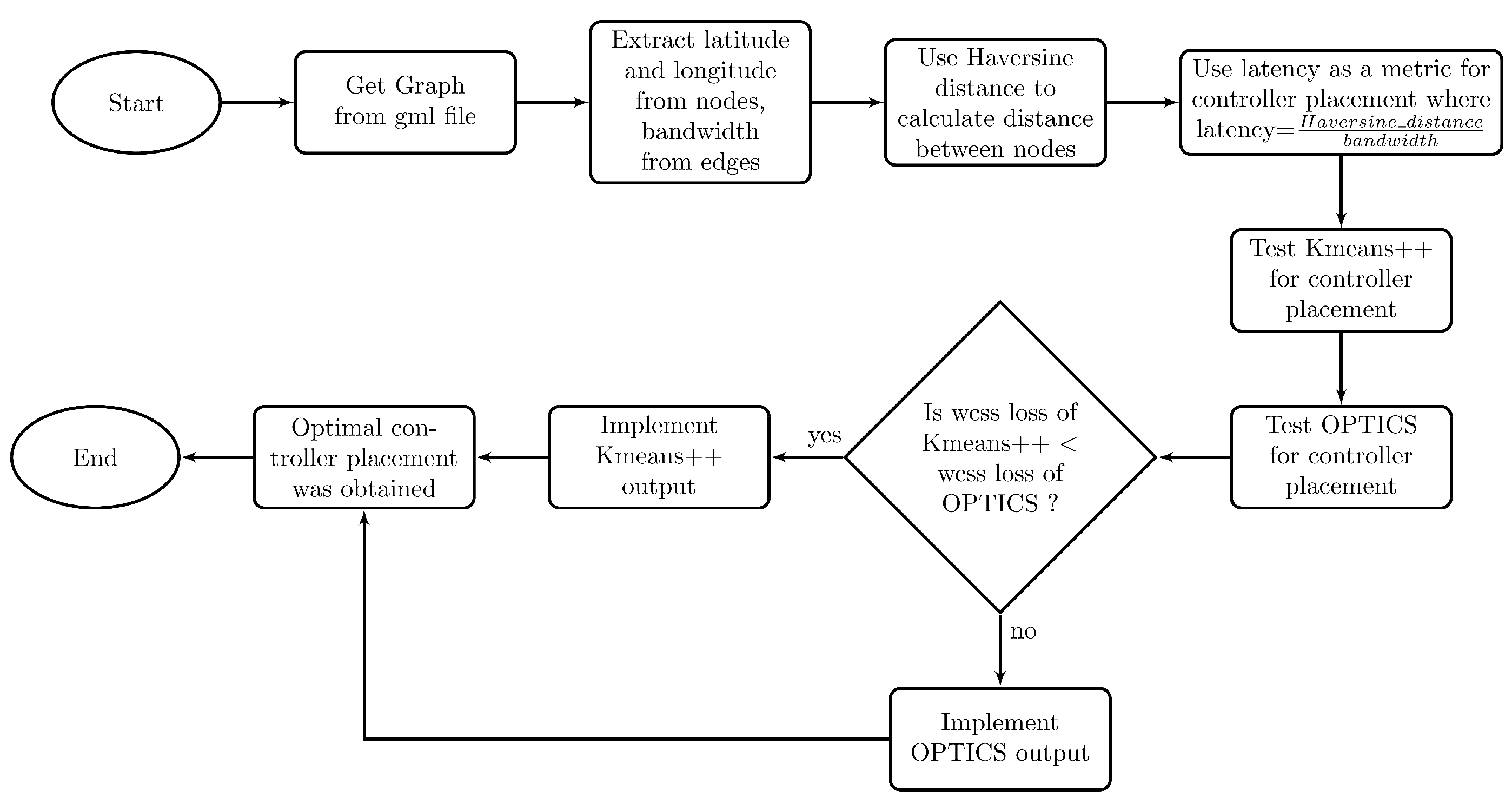
Figure 1 summarizes the process of determining the optimal controller placement. First, two GML files representing the topologies, Aarnet and Savvis, were downloaded from the Internet Topology Zoo [34]. From the files, the relevant parameters (Latitude, Longitude for the nodes and LinkLabel for the bandwidth of edges) were extracted. After this, using Haversine distance (Equation (2)) and latency (Equation (1)) metrics, Algorithm 1 was implemented, which tested each topology by two methods, namely, Kmeans++ and OPTICS. The WCSS losses from each method were compared, and the output from the method which yielded a lower WCSS loss was implemented for the implementation of the network containing optimally placed controllers, switches and hosts.

Figure 1. Flowchart for optimal controller placement implementation.

Figure 1. Flowchart for optimal controller placement implementation.

Algorithm 1 Controller Placement Algorithm.

Input: GraphG(V,E), radius = 6371 km /* Graph without controllers, where G = graph, V = set of vertices and E = set of edges */ /* For calculation of proximity between any two nodes, Equations (1) and (2) are used. */ /* GetNeighbors(v, Graph(vertex,edges)) returns all the vertices connected to v */ 1: L1 ← 0, L2 ← 0    ▷ L1 = WCSS loss using OPTICS, L2 = WCSS loss using K-means++ 2: G1(V,E), C1(V) ← OPTICS(G(V,E), d)    ▷ G1(V,E) = Graph with controller placement using OPTICS, C1(V) = list of controller vertices from OPTICS 3: G2(V,E), C2(V) ← Kmeans++(G(V,E), d) ▷ G2(V,E) = Graph with controller placement using K-means++, C2(V) = list of controller vertices from K-means++ 4: for  each v ∈ C1(V)  do 5:     U ← GetNeighbors(v,G1(V,E)) 6:     for each u ∈ U do 7:       L1 ← L1+d(u,v) 8:     end for 9:   end for 10: for  each v ∈ C2(V)  do 11:     U ← GetNeighbors(v,G2(V,E)) 12:     for each u ∈ U do 13:       L2 ← L2+d(u,v) 14:     end for 15: end for 16: if  L1<L2  then 17:     G(V,E) ← G1(V,E) 18:     L ← L1 19: else 20:     G(V,E) ← G2(V,E) 21:    L ← L2                                       ▷ L = Minimum WCSS loss value 22: end if 23: return $L,G(V,E)$

$$d(x_1,x_2)={\displaystyle \frac{Haversinedistancebetween{x}_{1}and{x}_2\left(inKm\right)}{bandwidthbetween{x}_{1}and{x}_2\left(inMbps\right)}}$$

(1)

where

$distance(x_1,x_2)=d(x_1,x_2),$

$x1=$ a node present in the selected graph (say node 1), and

$x2=$ another node present in the selected Graph (say node 2).

In Equation (1), latency is a function of $distance$, which is defined as how fast packets traverse between two nodes, and it is directly proportional to the physical distance separating these nodes. However, if the bandwidth between the nodes is increased, data transmission occurs at higher rates, resulting in reduced delay between consecutive packets, which is indicative of an inverse relationship.

And, the Haversine distance formula from Equation (2) calculates the shortest distance between two points on a sphere:

$$dH(lat1,lat2,long1,long2)=2\ast radius\ast arcsin\left(\sqrt{{\sin }^2\left({\displaystyle \frac{lat2-lat1}{2}}\right)+cos\left(lat1\right)·cos\left(lat2\right){\sin }^2\left({\displaystyle \frac{long2-long1}{2}}\right)}\right)$$

(2)

where

$Haversinedistance(lat1,lat2,long1,long2)=dH(lat1,lat2,long1,long2),$

$lat2=$ latitude of node 2,

$long2=$ longitude of node 2,

$lat1=$ latitude of node 1,

$long1=$ longitude of node 1,

$radius=$ radius of earth in kilometers.

From the topology, its graph G contains vertices V and edges E, where V represents $Latitude$ and $Longitude$, and edges contains the $LinkLabel$ attribute denoting the bandwidth between any two vertices. The C term represents controllers. The L term represents the minimum within-cluster sum of squares (WCSS) loss value. Algorithm 1 shows the implementation of K-means++ and OPTICS to obtain an optimal controller placement.

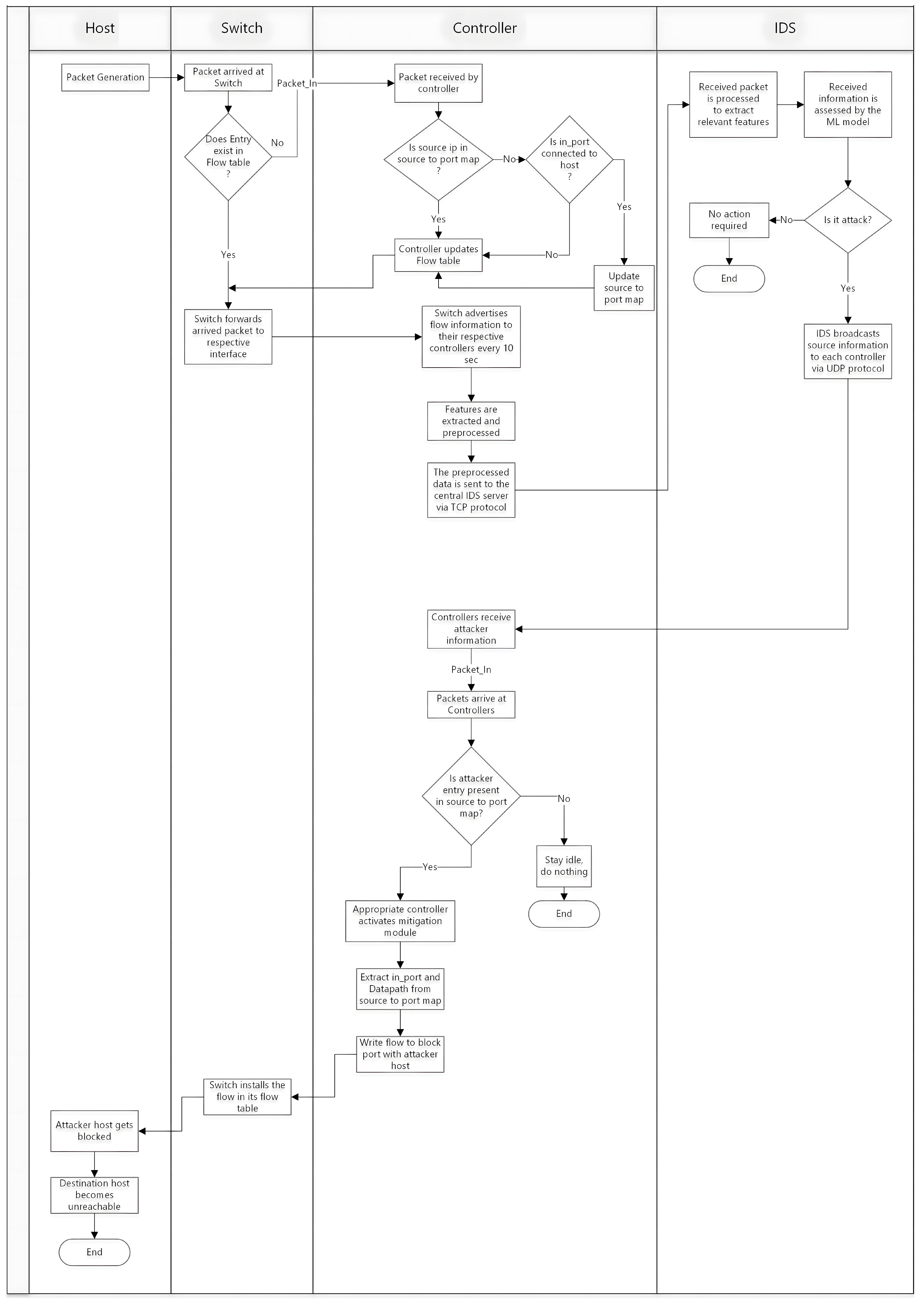
The workflow diagram of the designed system is shown in Figure 2. This diagram summarizes the entire workflow of network traffic (both benign and attack), providing a visual representation of how the multi-controller setup is organized to detect and mitigate DDoS attacks efficiently. The communication scheme between different components of the SDN environment, the host–switch, switch–controller, and controller–IDS is shown. A switch forwards the packets from a host to the respective interface using the flow table. Switches also advertise the flow information to their associated controller every 10 s. A controller does the job of managing the flow table of the switch and also performs feature extraction and pre-processing of the flow information, which will be sent further to the central IDS. IDS performs the task of classification of the traffic, benign/attack, and in case of an attack traffic, it broadcasts the attacker source information to each of the controllers. The controller with an attacker in its domain upon receiving this attacker information will activate the mitigation module and will request the installation of a flow in the respective switch to block the port of the attacker. The switch, upon receiving this request, will install this flow, and as a result, the attacker will be blocked for a predefined duration of 10 min. For normal traffic, no specific action is performed, and the traffic follows a normal natural route. A more detailed explanation on the detection and mitigation mechanism is provided in Section 3.9.

3.2. Development of Network Topology

GML files for Aarnet and Savvis topologies were downloaded from the Internet Topology Zoo [34]. K-means++ and OPTICS algorithms were used to determine the optimal number and positions for controllers. Controllers were placed at the centroids of each cluster such that a controller controls switches (nodes) falling in that cluster. We implemented an outband control mechanism, meaning data and control packets travel through different channels in the network. Following this, each node was assigned as an OpenFlow switch with a designated number, aligning them with the controllers determined by the clustering results from the best between K-means++ and OPTICS. This process resulted in an optimized SDN setup with strategically placed controllers and neatly assigned switches based on the clustering algorithm. Subsequently, two hosts were assigned to each OpenFlow switch and numbered as $(2\ast switch\_number-1)$ and $(2\ast switch\_number)$.

To manage communication between controllers, either controller–controller (C2C) links or a hierarchical control mechanism can be used. In this work, we employ the latter approach with IDS sitting on top of placed controllers, which manages control (like a global controller scenario) as well as application functions. The IDS manages control functions like handling duplicate IP addresses–IDS monitors IP addresses controlled by each controller, alerts the controller if two hosts share the same IP address, and relays attacker information between controllers and application functions, including attack detection using a trained ML model. In this paper, we discuss IDS mainly from the application function point of view because it is related to the use of ML algorithms for the detection of attacks.

3.3. Generation of Dataset

The DDoS attack SDN Dataset [35], designed specifically for SDN, was studied, and insights for relevant features were obtained. Also, the importance of the ICMP type was realized by studying experiments [36]. Our experiment was conducted on a Dell Laptop (i5, 16 GB RAM, Ubuntu 22.04.02 LTS 64 bit, Dell, Round Rock, TX, USA). Mininet (version 2.3.0.dev6) was used to emulate an SDN environment. For emulation, the IDS system, controller, switches, and hosts were turned active. The switch used here is an OpenFlow switch capable of supporting OpenFlow Protocol. The setup for attack/benign dataset generation can be seen in Figure 3. With these features in consideration, Savvis topology was used to generate Benign and DDoS-traffic containing datasets. These two datasets were later concatenated. Ping for ICMP and custom sockets for TCP/UDP were used for the Benign dataset. In the DDoS dataset, hping3 generates floods (ICMP, TCP, UDP) where each host can launch attack rates and bandwidths reaching up to 56 packets per millisecond and 10 Mbps, respectively.

For a benign dataset, a web server was hosted on host 5 and connected to a third switch in port number 3. A random source–destination pair (source! = destination) was chosen, and custom TCP and UDP servers were launched at the destination side. UDP and TCP data exchanges occurred between the source and destination for 5 s. Additionally, HTTP requests (GET and POST) were sent to the web server by source, and ICMP ping was carried out 50 times from the source to the destination. Flow statistics were advertised by switches to the controller at regular intervals; these controller data were transported to the IDS via TCP. The IDS appended data from each controller to a local CSV file with the process iterating until 100,000 benign samples were obtained. For malignant datasets, random source–destination pairs (source! = destination) were selected for each category of attack, and TCP and UDP servers were launched on the destination. We employed TCP SYN for protocol attacks and used UDP flood and ICMP flood for volumetric attacks. The source executed TCP SYN, UDP flood, and ICMP flood until the flows were active. The malignant dataset was appended to the benign dataset and sorted according to the time attribute. The merged dataset contains both types of data. To distinguish between an attack and normal data, labels 1 for attack data and 0 for benign data were assigned.

3.4. Details of the Dataset Generated

The generation of the benign dataset required 110 min. There are 19 columns and 100,718 rows in it. On the other hand, the malignant dataset required 8.3 min to generate. It contains 335,613 rows and 19 columns. After merging both, a total of 436,331 data samples were obtained with 19 features and a size of 53.69 MB. The attributes of this dataset are shown in

Table 1. Details of the generated dataset.

Column Number	Feature Name	Description
0	$time$	time of arrival at the controller
1	$switch\_id$	datapath ID of switch
2	$ip\_src$	source IP address
3	$src\_port$	TCP or UDP port number
4	$ip\_dst$	destination IP address
5	$dst\_port$	TCP or UDP port number
6	$ip\_proto$	IP protocol
7	$icmp\_type$	type of ICMP packet
8	$flow\_duration\_sec$	active time period of flow in sec
9	$flow\_duration\_nsec$	active time period of flow in nsec
10	$remaining\_idle\_time$	remaining idle time of flow
11	$remaining\_time$	total remaining time of flow
12	$packet\_count$	total packets
13	$byte\_count$	total bytes
14	$packet\_count\_per\_second$	number of packets in 1sec
15	$packet\_count\_per\_nsecond$	number of packets in 1nsec
16	$byte\_count\_per\_second$	number of bytes in 1sec
17	$byte\_count\_per\_nsecond$	number of bytes in 1nsec
18	$label$	benign (0) or attack (1)

. Columns 0 to 17 represent independent features, and column 18 is the dependent feature.

To the best of our knowledge, this dataset is the first collected in a multi-controller environment and does not require any packet capturing or monitoring overhead, which would add unnecessary strain on the controller. Instead, this dataset relies solely on reading the statistics from flow tables provided by OpenFlow switches. This approach helps reduce congestion in the control plane, unlike those that utilize CIC datasets.

3.5. Dataset Preprocessing

To refine the dataset, several steps were undertaken. First, rows with $nan,inf,-inf$ values were eliminated. The entire dataset was sorted based on the time attribute for better organization. Feature selection was performed, and irrelevant columns—namely, columns 1, 2, 3, 4, and 5—were dropped, which was guided by correlation analysis to extract meaningful insights. Now, all data were already in numeric format, so no additional numericalization was required. The dataset was then split into training (80%) and testing (20%) sets followed by normalization of the training and test set. Finally, to address binary class imbalance and prevent any over-reliance of labeled data in multi-controller environments, random undersampling was applied. The processed dataset was then used for training ML models and also for testing the performance. The best-performing model was used for the IDS system.

3.6. Machine Learning Algorithms Used for Training Dataset

ML, a subfield of artificial intelligence, focuses on the development and use of statistical algorithms to generalize from data and perform tasks without explicit programming. ML algorithms have been widely applied to various classification and prediction problems. In our study, several classification algorithms were evaluated, namely, Naive Bayes, XGBoost, KNN, random forest, neural networks (NNs), and LSTM. The NN model was implemented with three sequential layers using ReLU and Sigmoid activation functions along with the Adam optimizer. The input layer consisted of 13 neurons to process features from the dataset, while the second layer contained 32 neurons with ReLU activation. The output layer had a single neuron with Sigmoid activation for binary classification. The model was trained using binary cross-entropy as the loss function, running over 100 epochs with a batch size of 10,000.

The LSTM model was developed using a sequential architecture. Its first layer included a bidirectional LSTM, which processed input sequences in both forward and backward directions, capturing past and future contexts. This LSTM layer consisted of 64 units, used the hyperbolic tangent (tanh) activation function, and applied L1 regularization. A second, fully connected dense layer with 128 units employed the ReLU activation function and L2 regularization. The output layer featured a single neuron with Sigmoid activation for binary classification. As LSTM works on time series data, individual instances from our dataset need further manipulation to be considered time series. Therefore, a sliding window approach [37] was adopted for both the training and testing phases. A window size of 25 (an arbitrary assumption) was used with each training instance being all instances within this window. This method enabled the training dataset to be processed as a time series. The same procedure was applied to the test set. If implemented in an IDS, an LSTM processes frames using a window of 25; if a frame contains fewer than 25 instances, the LSTM generates results based on the available instances. The random forest model was configured with 10 estimators and used entropy as a loss metric. For the KNNs algorithm, the hyperparameter was set to 3 neighbors.

3.7. Data and Control Plane Communication

The obtained topologies comprised multiple paths between hosts. To address this problem, the topology was transformed into a minimum spanning tree based on the distance ($X_1,X_2$) metric, as shown in Equation (1), to eliminate redundant paths. Each host received an IP address beginning with 10.0.0.1 and an MAC address starting from 00:00:00:00:00:01. Afterwards, the switch–switch bandwidth was configured according to the dataset [34]. The bandwidths for the switch–host, switch–controller, and controller–IDS connections were set based on the maximum and minimum bandwidth between switches. The switch–host bandwidth was equal to the minimum bandwidth between the switches, while switch–controller bandwidths were equal to the maximum bandwidth between switches, and the controller–IDS bandwidth was set to k times the maximum bandwidth between switches, where k represents the number of controllers. The controller–IDS bandwidth was chosen to be k times the maximum switch–switch bandwidth, as data from multiple switches are to be sent to the IDS via the controller, and any lesser bandwidth may lead to bottlenecks. Similarly, the minimum bandwidth was used for hosts to control congestion to an extent during a DDoS attack. This implemented minimal bandwidth is sufficient for benign traffic. Ryu controllers were programmed to map the IP address and port number in OpenFlow switches. The mapping enables the switches to relay messages between terminals. Furthermore, the switches replied with flow table statistics to their respective controllers every 10 s. In our case, controllers only process the forward-flow (Tx) advertisements to pass on to the IDS. Controllers ignore the flows created in response to requests like ICMP and TCP. This ensures that flows in only one direction are processed and prevents false alarms due to burst reply packets.

3.8. Controller–IDS Integration

Using Mininet, controllers were strategically placed, and they were each assigned a consecutive IP address starting from 127.0.0.2. Additionally, a dedicated host was emulated for testing IDS functionality with the IDS being placed at the center of all controllers. To facilitate communication and the transfer of CSV data between the controller and IDS, a TCP server on port 9998 was initiated on the IDS. Once the file transfer was completed, the connection was terminated. Subsequently, a new TCP server on port 9999 was established on the IDS to receive flow-statistics data intended for AI models.

IDS upon predicting the received data as either an attack or normal information containing the attacker’s IP address was encapsulated into a UDP datagram. This datagram was then sequentially sent to each controller to port 8888 if the prediction indicated an attack. If the prediction was normal, no information was sent to the controllers.

Congestion represents a critical factor in determining the efficacy of an IDS. The persistent transmission of messages from switches to the controller or packet-capturing devices are well known to cause congestion in the control plane. To mitigate this issue, we implemented a multi-controller environment with controllers positioned strategically. In this setup, flow advertisements from switches are only transmitted to their respective controllers. Thus, no single controller is burdened by a substantial volume of advertisements from the data plane, providing some level of load distribution among controllers. Additionally, the use of the UDP protocol for decision packets ensured minimal congestion in the controllers. During a DDoS attack, the controller resources could be compromised, and utilizing TCP would lead to numerous retransmission packets, thereby delaying mitigation efforts. Consequently, UDP addresses this issue by encapsulating a compact packet without any retransmission overhead. Algorithm 2 shows that the IDS will always respond with a decision packet as long as the DDoS attack is on, implying that even if some UDP packets are lost, subsequent responses will cover this limitation without retransmission. These considerations ensure communication and coordination with minimum delay, allowing real-time threat detection and instant reply by controllers.

Algorithm 2 IDS Detection Algorithm.

Input: Flow Packet, $C_n$  threshold = 5 1: victim[ ] ← NULL 2: while  IDS is active  do 3:   Receive flow statistics from controllers every 10 s 4:   Frame ← Extract_features() 5:   for data ∈ Frame do 6:    prediction ← XGB.Predict(data) 7:    if prediction=1 then 8:     victim[data.dst_ip] ← (data.src_ip,count+1) 9:    end if 10:    Attack_source,Attack_destination ← GetMax_count(victim) 11:    victim[Attack_destination].count ← 0 12:    IDS.sendall($C_n$, Attack_source) 13:    Reset victim every 150 s 14:   end for 15: end while

In Algorithm 2,

$C_n=$ list of controller IP addresses,

$Extract\_features\left(\right)$ extracts relevant features from the flow statistics packet,

$XGB.Predict\left(\right)$ classifies benign/attack using XGBoost, and

$GetMax\_count\left(\right)$ returns the source IP of entry having the maximum count and exceeding the minimum threshold

Algorithm 2 describes the IDS detection process during a DDoS attack. An empty victim list is initialized in IDS. The IDS continuously monitors the flow statistics received from the controllers, which is updated every 10 s. The flow information originated from the Open flow switches, and it makes it up to the IDS via the respective controllers. The IDS extracts relevant features from the frame for analysis. Using XGBoost, each flow is classified as either a benign traffic (label 0) or an attack traffic (label 1). If an attack is detected, the attack count for the victim (using the destination IP) is increased. The function GetMax_count() finds the source IP that has attacked the victim the maximum number of times. At this point, the attacker IP to be blocked is well determined. Now, the victim count is reset, and IDS broadcasts the source IP to all the controllers. After every 150 s, the victim list is reset to free up memory and to prevent false positive for any legitimate traffic. However, once the IDS broadcasts the source IP, flagging it as an attacker, it will remain blocked for 10 min.

3.9. DDoS Attack Detection and Mitigation in Emulated SDN Environment

A custom DDoS Python script with spoofed IPs using a Scapy library (v. 2.4.4) was launched from one of the hosts. This script differs from the one applied in dataset generation because the attack rate (up to 30 packets per second) varies in comparison to the hping3 attack rate (up to 56 packets per millisecond) utilized for generating the dataset. The rate was varied to assess the generalizing capability of the trained model. When a source host in an SDN generates attack traffic, this traffic is routed toward the victim host via intermediate switches. Every switch through which this attack packet goes reports the packet’s flow statistics to its respective controllers. Upon obtaining the flow statistics, each controller processes the data by transforming numerical values into the floating point and encapsulating them for further transmission; then, it sends the processed statistics to a centralized common IDS. IDS, after receiving the stats from controllers, extracts relevant processed features from the frame, and using those features, it makes a prediction using the XGBoost algorithm. If the model predicts an attack (prediction value of 1), it updates the source IP as a potential attacker for the corresponding destination IP (IP address of the receiver), and the victim counter is increased by 1. This counter can be updated due to the flow received from any of the controllers. This counter keeps track of how many times this destination IP was flagged as victim. Finally, the algorithm identifies the attacker source IP with the highest victim count exceeding the threshold of minimum detection and sends this information to all the controllers. This counter strategy was used to reduce false positives during detection. An IP is flagged as malicious only after surpassing a threshold of minimum detection (set to 5), reducing the likelihood of blocking legitimate traffic. If the threshold is set high, the attack is persistent, increasing false negatives. Conversely, if the threshold is low, false positives increase. This parameter can be adjusted according to the use case and type of network. We have set its value to 5 as an arbitrary assumption. Additionally, the system resets counters periodically to ensure efficient memory usage.

The controller, upon receiving information about an attacker and a victim, stores the information. The controller’s mitigation module possesses a mapping of source IP addresses to their respective datapaths and in-ports. If there is no record of the source IP in the map and it is from a port connected to the host, the controller adds it to its map. Now, the controller associated with the attacking host has the entry present for the attacking host in the map, ensuring that the blocking mechanism is activated only by the appropriate controller. Upon the triggering of a packet-in event, the controller assigned to the switch with the source host can efficiently retrieve datapath and in-port information from the dictionary. Subsequently, the controller initiates the creation of a flow entry to block traffic on the specified interface, leading to a blockage of DDoS traffic from the source host. 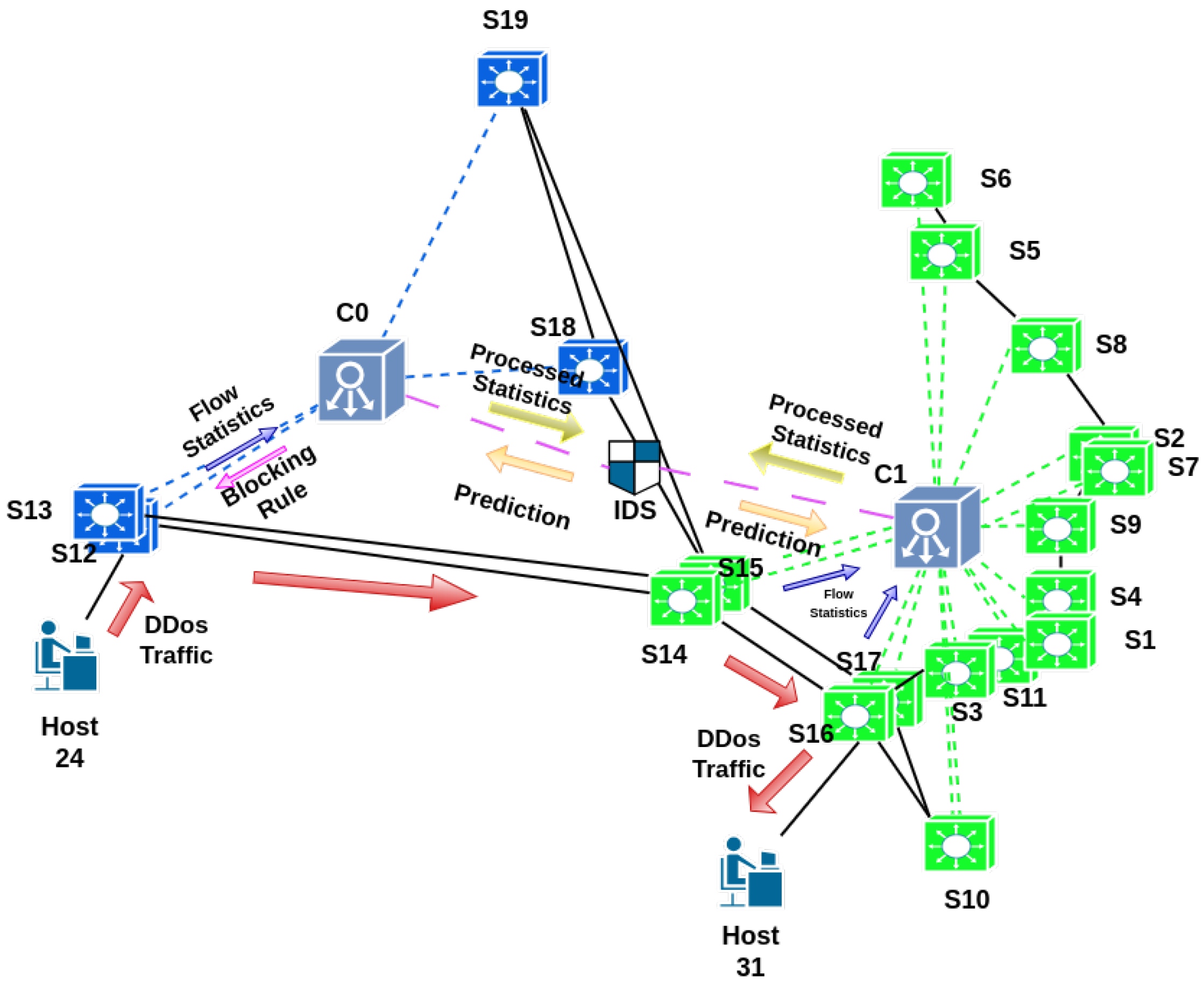This process has been depicted in Figure 3 through a system diagram.

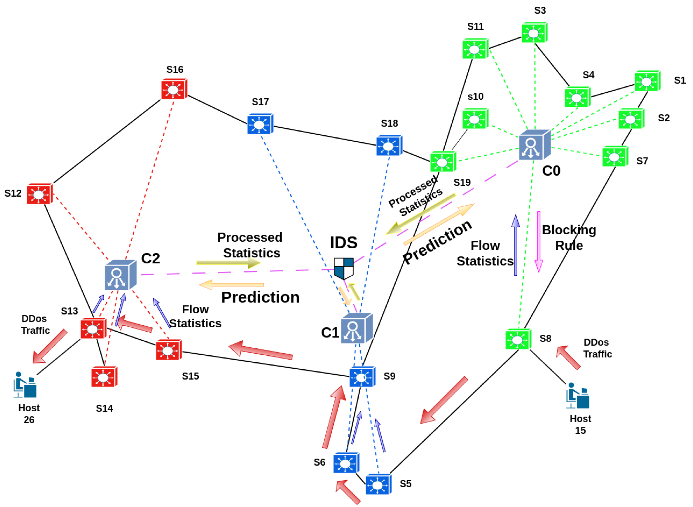
Figure 3 illustrates the attack generation, detection and mitigation process in a multi-controller environment. The segregation of three planes in SDN—the control, data and application plane—is shown. Host and openflow switches lie in the data plane; controllers lie in the control plane and the central IDS lies in the application plane. The cluster area represents the domain of a controller. Communication between switches and the controller is via southbound APIs, and that between controllers and IDS is via northbound APIs. When a host generates DDoS traffic intended to another host located in a different cluster, firstly, the packet goes through the associated switch. The switch then forwards flow information to its respective controller (here, controller 1). Controllers process the statistics and pass it on further to the central IDS. IDS uses this processed information in the XGBoost algorithm and makes a prediction. If the prediction classifies the traffic as an “attack”, this prediction is relayed to all the controllers. The controller with the attacking host in its domain installs a blocking rule in the switch, and eventually, the attacker is blocked.

To ensure optimal performance, prevent memory exhaustion, and restore blocked devices, the dictionary is cleared at regular intervals—specifically, every 10 min. This periodic clearing of the dictionary helps maintain system efficiency and prevent the degradation of network performance. The entire process of detection and performing mitigation takes a minimum of 0 s and a maximum of 10 s. We trained a model using a dataset from Savvis topology, and this trained model was used for the detection and mitigation of DDoS attacks in both Savvis and Aarnet networks to study the generalization of our algorithms.

In Algorithm 3,

-

$C_n$ = list of controllers,

-

$C_i$.store() stores the received IP into memory,

-

controller.load() loads stored IP from the memory,

-

controller.erase() clears the memory,

-

controller.block() creates flow entry to block the DDoS traffic.

Algorithm 3 Attack Mitigation Algorithm.

Input: Attacker IP Address, $C_n$ 1: functionAlert_Controller: 2:   for $C_i$ ∈ $C_n$ do 3:    Source_ip ←$C_i$.receive(IDS) 4:    $C_i$.store(source_ip) 5:   end for 6:   return None 7: end function 8: function  Mitigation_Module: 9:   port_map[ ] ← NULL 10:   Packet_In_Event 11:   (datapath,switch_id,src_ip,in_port)← Extract_features() 12:   if in_port is connected to a host then 13:    port_map[source_ip] ← (datapath,in_port) 14:   end if 15:   attacker ← controller.load() 16:   if attacker in port_map then 17:    controller.block(port_map[attacker].datapath, port_map[attacker].in_port) 18:    controller.erase() 19:   end if 20:   Reset port_map every 10 min 21:   return None 22: end function

Algorithm 3 shows how a controller blocks an attacker. The ALERT_CONTROLLER function receives broadcasts from the IDS in an event of attack and stores the source IP in the controller. This algorithm is run in all of the controllers, so all of them store the attacker’s IP. Now, the next function MITIGATION_MODULE becomes functional. An empty port_map dictionary is initialized which, will be used to store the datapath (the switch) and the in_port (the switch port where the packet entered). When a packet arrives (realized by the packet_in event), the controller extracts relevant details: namely, datapath (unique OpenFlow identifier assigned to a switch), switch_id (general name of a switch), src_ip (the source ip of the attacker), and in_port (the switch port where the attacking packets entered). Now, if the in_port is connected to a host (not to some other switch), then the port_map dictionary stores the value (datapath, in_port) to the source_ip key. The controllers retrieve the attacker IP (source_ip) and store it in the variable $attacker$.

If any key in the port_map matches with $attacker$, it means that the attacking host lies in the controller’s domain, and if there is no match, then the controller will remain idle, since the attacking host is not in their domain. For the controller containing the attacking host, a blocking rule to block DDoS traffic is created by a flow entry using the controller.block() module. Only the associated switch (identified from the datapath) installs this blocking flow in its flow table. As soon as this flow is installed, the attacking host becomes blocked. Meanwhile, the controller deletes old attack records from its memory using controller.erase(), ensuring its memory is not overloaded. After a period of 10 min (an arbitrary assumption), the port_map dictionary is cleared. This prevents some genuine traffic from being blocked indefinitely. However, if the attacker still continues to send DDoS traffic, it will again be flagged and blocked by the same mechanism.

4. Results and Discussion

4.1. Algorithm Performance for Optimum Multi-Controller Placement in Aarnet

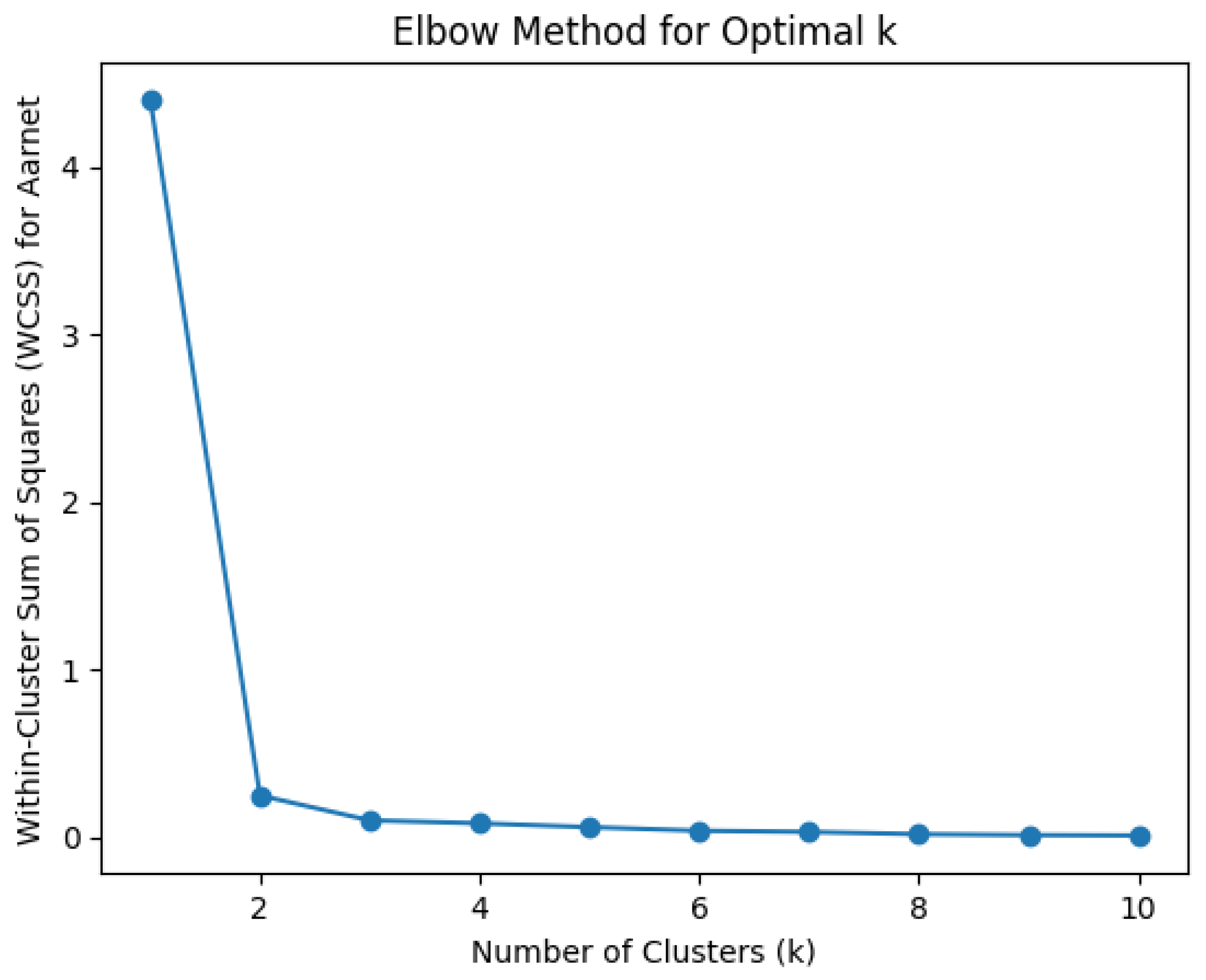
For an unsupervised algorithm, determining the optimal number of clusters is a fundamental step. The elbow method identifies the optimal value of centroids (k) for the K-means++ algorithm. Similarly, we used grid search to determine the optimal value of centrioids using OPTICS.

We performed a continuous iteration for k = 1 to k = 10, and for every value of ‘k’, WCSS was calculated. It provides the sum of square distances between each location and the centroids. A graph of k versus their WCSS value is plotted in Figure 4, which resembles an elbow. To identify the optimal number of clusters, the value for ‘k’ must be selected at the “elbow” point; this is the point where the distortion starts decreasing in a linear fashion [38]. For k = 2, two controllers, $c_0$ and $c_1$ were placed, yielding a WCSS loss of 0.1750, as shown in Figure 5.

Running OPTICS on Aarnet yielded a similar configuration as produced by K-means++ with two clusters and a WCSS loss of 0.2012. Hence, two controllers $c_0$ and $c_1$ were placed, as shown in Figure 6.

Inference: Since (WCSS loss of K-means++) < (WCSS loss of OPTICS), the result from K-means++ was implemented for Aarnet, yielding two clusters, as shown in Figure 6 and Figure 7. Figure 7 is a more detailed diagram of the implementation of Aarnet topology.

4.2. Algorithm Performance for Optimum Multi-Controller Placement in Savvis

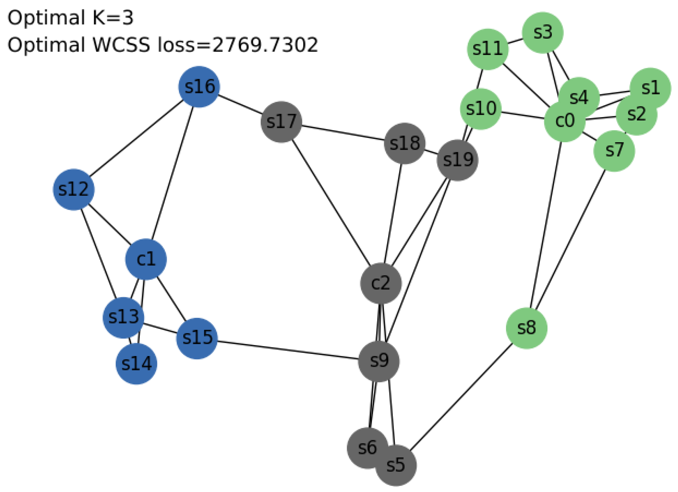
Similarly, running K-means++ in Savvis resulted in an elbow at k = 3 with a loss of 2769.7302, as shown in Figure 8. Hence, controllers $c_0$, $c_1$, and $c_2$ were placed accordingly, as shown in Figure 9. Again, running OPTICS on Savvis also yielded a configuration with three controllers, as depicted in Figure 10 with WCSS.

Inference: Since (WCSS loss of OPTICS) < (WCSS loss of K-means++), the result from OPTICS was implemented for Savvis, yielding three clusters in Figure 10 and Figure 11.

The WCSS in Savvis is relatively high compared to that of Aarnet. This difference can be attributed to the variation of link speeds in these networks. In Aarnet, the link speeds are typically in the order of gigabits per second (Gbps), whereas in Savvis, they range in the order of megabits per second (Mbps). This factor accounts for a larger denominator in Aarnet compared to Savvis in Equation (1), resulting in a smaller distance for Aarnet.

After controller placement optimization, Figure 7 and Figure 11 represent the resulting system diagram incorporating controllers, switches, and the central IDS along with the flow of actions. The arrows show the direction and type of packets flowing in the environment, whereas the lines represent the physical connections between the devices. Meanwhile, the system can detect and mitigate attacks appearing from multiple hosts simultaneosly. For simplicity and clarity, we have illustrated an attack from only one host in Figure 7 and Figure 11. DDoS is used despite there being a single host due to the host using multiple spoofed IPs for the attack.

4.3. Performance Evaluation of ML Models

The computation time and accuracy are key factors that define the performance of an IDS. Therefore, the performance of ML models was assessed based on test time, which refers to the time taken to process the entire test set, as well as their accuracy, including precision, recall, and F1-score.

From

Table 2. Performance in terms of train–test time and train–test accuracy in terms of percentage.

Model	Train Time	Test Time	Train Acc.	Test Acc.
Random Forest	946 ms	106 ms	98.65	97.00
XGBoost	728 ms	70 ms	97.3	98.5
Naive Bayes	54 ms	42 ms	67.7	91.53
KNN (n = 3)	198 ms	126 ms	94.51	93.32
NN	11.6 s (50 epochs)	4s	91.62	93.6
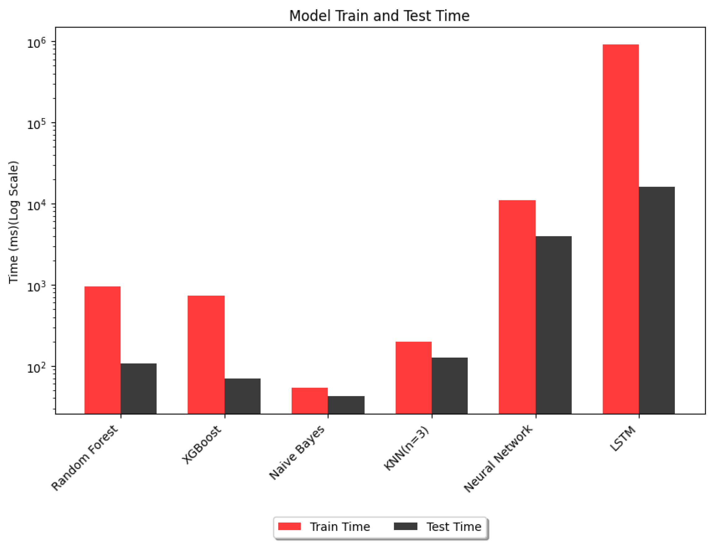
LSTM	15 m (15 epochs)	16s	99.9	99.9

, it can be observed that random forest, XGBoost and LSTM offered greater than 95% test accuracy; this solves the detection part. However, to perform swift mitigation, a quicker response is equally important, and this faster response time has set XGBoost apart from others. The training accuracy of Naive Bayes was notably lower, as indicated in Figure 12, and a particularly low recall rate. Consequently, we decided not to continue with Naive Bayes. On the other hand, KNN exhibited a relatively longer test duration (Figure 13) and a low recal rate. A lower recall rate for both Naive Bayes and KNN is shown in (Figure 14) for benign traffic.

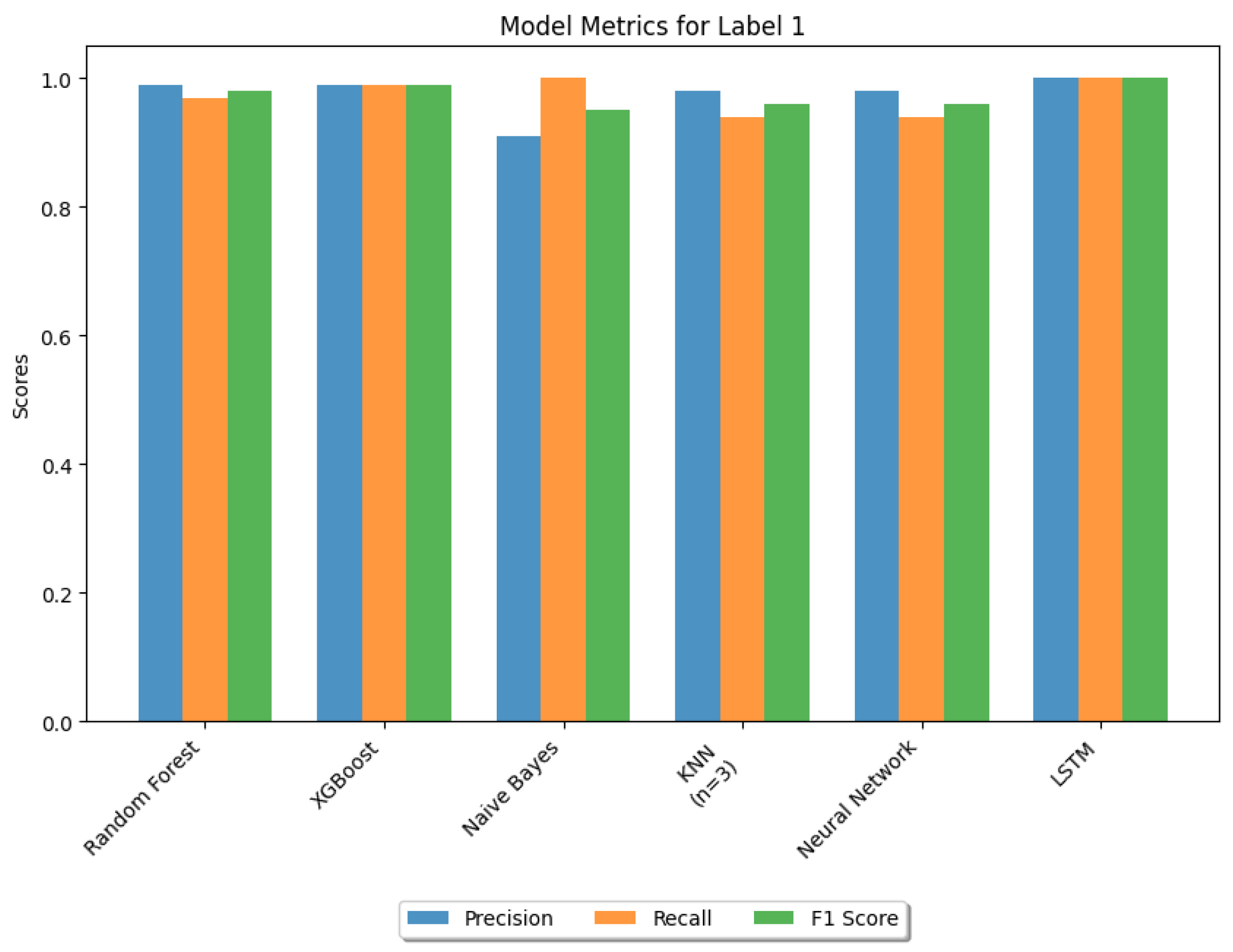
Figure 14 and Figure 15 compare the similar performance of algorithms, random forest and XGBoost, based on test accuracy and test time. Although both algorithms exhibit identical precision for label 1 (DDoS traffic), XGBoost demonstrates a higher recall for DDoS attacks. This indicates that among all actual positive instances of DDoS attacks, XGBoost can predict a greater number of attacks successfully. Consequently, XGBoost achieves a higher F1-score, reflecting a better balance between precision and recall.

Therefore, as XGBoost offered both an optimum balance of test accuracy (98.5%) and test time (70 ms) for our detection mitigation system, based on these results, we implemented XGBoost in our IDS to maximize the system performance.

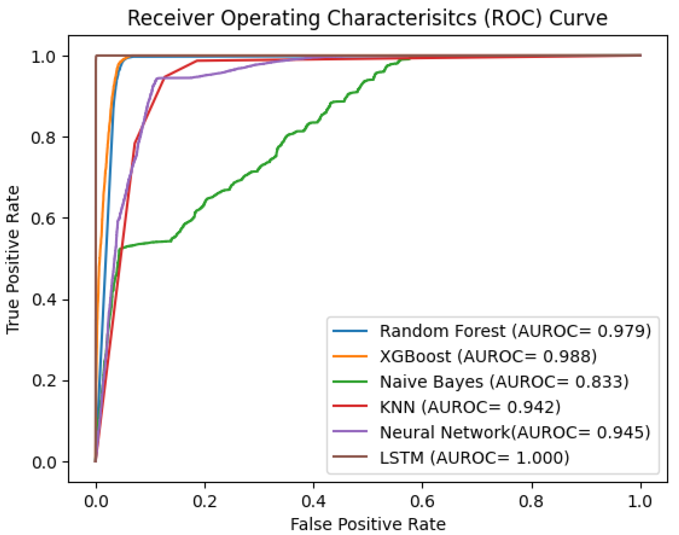
The receiver operating characteristic (ROC) curve depicted in Figure 16 reveals findings that support Table 2. Better classifying algorithms have a strong inclination toward the top left corner. Complex deep learning models such as LSTM outperformed other models. But despite the best performance, for our case, it took a significantly high prediction time of 16 seconds to classify the same data in comparison to XGBoost, which took 70 ms. The high testing time is proportional to the decision time of the IDS. If LSTM had been implemented, it would have resulted in a higher response time due to the time-series nature and sliding window methodology, which adds additional computational overhead. Therefore, it is not suitable for near real-time detection and mitigation. Consequently, LSTM was not implemented in our model.

From

Table 3. Comparison with recent works on DDoS detection.

Author	Domain	Dataset	Accuracy	Precision	Recall
Gebremeskel et al. [25]	Logically Single Distributed Controllers	CICDDoS Dataset	99.42	99.40	99.46
Clinton et al. [39]	Single Controller	InSDN Dataset	99.74	99.74	99.74
Al-Dunainawi et al. [40]	Single Controller	Custom Dataset	99.99	99.99	99.99
Hirsi et al. [41]	Single Controller	Novel Dataset	98.97	98.33	96.37
Alubaidan et al. [42]	No SDN Setup	DDoS SDN Dataset	99.50	99.40	99.50
Our model	Optimally Placed Multi-Controller	Flow Table-Based Custom Dataset	98.50 (Optimal) 99.99 (Best)	97.00 (Optimal) 99.99 (Best)	97.00 (Optimal) 99.99 (Best)

, the data presented demonstrate that our work point to a significant improvement in multi-controller DDoS detection. While several studies, such as Clinton et al. [39] and Ai-Dunainawi et al. [40], achieved strong results with respect to accuracy, precision, and recall in single-controller setups, our LSTM model with 99.9% test accuracy has achieved what we believe to be state-of-the-art performance, particularly in the more complex multi-controller context. Specifically, we mentioned only the InSDN dataset from the work by Clinton et al. [39], as it best represents the SDN environment, although other datasets were also considered in their paper. Compared to a single-controller setup, a multi-controller SDN setup is more complex. In the case of a single controller scenario, for an attack mitigation action, both the source and victim are present inside the domain of the same controller. This setup of a simple detection and mitigation algorithm can be executed on the single controller (simple algorithm in the sense that with a lesser number of controllers involved, there will be fewer things to take care of and the use cases are also relatively narrow for practical cases). However, when either an attacker or a victim lies in a separate domain, single controller algorithms cannot be employed because a coordinating mechanism is required between controllers. To address this problem, we need a more advanced mechanism where attacks from different controller domains can also be handled. For this, we implemented Algorithms 2 and 3 in a multi-controller environment. This setup naturally forms a complex network with the necessity of a more advanced algorithm, since data from domains of multiple controllers should be looked at while making decision and multi-controllers should also be in correlation (via IDS) such that mitigation is performed by precisely locating the attacker. Furthermore, controller placement considerations [28] are also important while dealing with multi-controller environments, adding extra complexity.

Furthermore, our optimal XGBoost model achieved an accuracy that is only 1.49% lower than the best models. This shows that despite focusing on both detection and mitigation while considering both accuracy and latency, our approach delivers competitive performance compared to models that prioritize accuracy alone. Additionally, our dataset differs from those of the mentioned models, as it is the first dataset collected in a multi-controller environment and contains different feature sets, marking a considerable contribution to the field of SDN DDoS security.

While the comparison metrics (accuracy, precision, and recall) of the mentioned works in the Table 3 are very similar, the major contrasting factor of our work is the setup of the SDN environment. Our setup of multi-controllers and a primary dataset, differing from other research, for the ML model provides a more closer resemblance to real-world scenarios. Despite the complicated setup of a multi-controller environment with a central IDS trained using a primary dataset obtained from SDN itself, our performance metrics manages to stand on par with the recent works on SDN DDoS security.

The notable thing in our work is we have indeed made use of simpler attacks (ICMP, TCP SYN, UDP flood attacks), which could have been easily resolved by simpler non-ML algorithms like entropy methods, bandwidth probes, hybrid statistical methods, etc. We went with an ML-based approach to exploit its learning capabilities. Traditional algorithms that are mostly threshold-based seem to need manual tuning to adapt to different rates of attacks. Hence, to eliminate the necessity of any manual tuning, we utilized the ML approach, which was also able to detect attacks efficiently. Additionally, we aim to establish a base framework of ML on this flow table-based dataset in a multi-controller environment. The detection of advanced attacks like LDDoS, ping of death, and application layer DDoS are kept as future works on this new framework.

4.4. Attack Detection and Mitigation

After XGBoost was deployed in both Savvis and Aarnet networks, our mitigation and detection algorithm were verified by two separate cases, namely, with and without the mitigation module. In the presence of a DDoS attack, it is expected for the victim to have a high number of incoming packets. Without the mitigation module in action, a high number of packets from the DDoS attack are being sent to the victim, as evident in Figure 17 and Figure 18.

With the mitigation module in action, there is a significant reduction in the number of packets, as shown in Figure 19 and Figure 20. There were fewer counts from the DDoS attack being sent to the victim, hence preventing the attack. Also, from Figure 21, it can be observed that CPU utilization increases significantly at the instance of DDoS attack (from time 12:51:00–12:51:30), and after the application of the mitigation module, it returns back to the normal state.

Figure 19, Figure 20 and Figure 21 demonstrate that our model effectively detects and mitigates attacks in multi-controller environments. Additionally, normal service is re-established as soon as the attack is over. Figure 19 and Figure 20 illustrate that aside from the largest/broadest spike, approximately from time 41 s to 59 s in Aarnet and from time 49 s to 58 s in Savvis, there is normal packet exchange. After the attack ends, the network continues with packet exchanges, as indicated by the smaller/thinner spikes that appear afterwards. This detection and mitigation address the limitations of previous models, which were either specific to certain topologies or focused solely on attack detection without considering network optimization. Furthermore, our algorithms showed strong generalization across both Aarnet and Savvis topologies; we used datasets generated from Savvis for testing in the Aarnet environment. This also confirms the robustness of our model.

Our work mainly focused on end host-to-host attacks. For the cases of attack against a controller, the flow generated is treated similarly like an attack to a host, and it can be detected and mitigated using the same previous approach and algorithms. But in the case of IDS, a host cannot launch a DDoS attack directly against it, because in our setup, the IP address of the central IDS is not made accessible to the end hosts.

5. Conclusions

This study focused on optimized multi-controller placement and an efficient DDoS attack detection mitigation system. Our approach ensures rapid detection and mitigation with response time ranging from 0 to 10 s as the controllers are programmed to advertise the flows every 10 s. By emphasizing practicality and efficiency, we made use of real-life topologies consisting of multiple controllers and optimized controller placement, and we developed an algorithm for an independent unit of IDS featured with the best-performing ML model for DDoS detection. Additionally, we developed an attack mitigation algorithm with a resource-efficient robust defense system with minimal computational overhead on controllers. For achieving DDoS attack detection and near real-time mitigation, the flow table was advertised by each switch every 10 s to their respective controller. This information was further processed by the controllers and passed to the IDS via TCP. The IDS, on receiving this, predicts a binary classification using the XGBoost algorithm and broadcasts it back to all controllers. With this information, the appropriate controller activates its mitigation module and blocks the malicious hosts in near real-time duration. In this way, the proposed model used Kmeans++ and OPTICS to obtain an optimized controller placement for a topology with multiple controllers, and the developed system was able to both detect and perform a near real-time mitigation of DDoS attacks with an accuracy of 98.5%.