Article

Unsupervised Machine Learning Techniques for Detecting PLC Process Control Anomalies

by
Emmanuel Aboah Boateng
and
J. W. Bruce
*
Department of Electrical and Computer Engineering, Tennessee Technological University, Cookeville, TN 38505, USA
*
Author to whom correspondence should be addressed.
J. Cybersecur. Priv. 2022, 2(2), 220-244; https://doi.org/10.3390/jcp2020012
Submission received: 14 February 2022 / Revised: 11 March 2022 / Accepted: 17 March 2022 / Published: 24 March 2022
(This article belongs to the Collection Machine Learning and Data Analytics for Cyber Security)

Abstract

:
The security of programmable logic controllers (PLCs) that control industrial systems is becoming increasingly critical due to the ubiquity of the Internet of Things technologies and increasingly nefarious cyber-attack activity. Conventional techniques for safeguarding PLCs are difficult due to their unique architectures. This work proposes a one-class support vector machine, one-class neural network interconnected in a feed-forward manner, and isolation forest approaches for verifying PLC process integrity by monitoring PLC memory addresses. A comprehensive experiment is conducted using an open-source PLC subjected to multiple attack scenarios. A new histogram-based approach is introduced to visualize anomaly detection algorithm performance and prediction confidence. Comparative performance analyses of the proposed algorithms using decision scores and prediction confidence are presented. Results show that isolation forest outperforms one-class neural network, one-class support vector machine, and previous work, in terms of accuracy, precision, recall, and F1-score on seven attack scenarios considered. Statistical hypotheses tests involving analysis of variance and Tukey’s range test were used to validate the presented results.

Graphical Abstract

1. Introduction

The pervasiveness of Internet of Things technology and networked sensors in many industrial control systems (ICSs) have exposed critical infrastructure to malicious activities and cyber threats, leading to an increase in successful cyberattacks on critical infrastructure [1,2,3,4]. Programmable logic controllers (PLCs) are embedded devices that serve as major components in ICSs and are crucial to ICSs’ network operation. PLCs control industrial systems by collecting input data from field devices such as sensors and sending commands to actuating devices for process execution [5,6]. ICSs monitor and control critical infrastructure such as nuclear facilities, electricity supply, and water management. PLCs are vulnerable to attacks, similar to other embedded devices. Because PLCs are widely used to control the physical processes of critical infrastructure, attacks against PLCs can cause irreparable damage to enterprises and even loss of human life [7].
In the past, PLCs operated as isolated and proprietary systems with no external connectivity [8,9]. As a result, PLC attacks were limited to insider intrusion, physical damage, and tampering [10]. PLCs are increasingly connected to the internet and corporate networks via transmission control protocol/internet protocol (TCP/IP) and wireless IP [11]. It is difficult to apply traditional techniques for detecting anomalous PLC behavior due to their unique architecture and proprietary operating systems. Therefore, it is crucial to protect PLCs against any forms of cyber-attack and anomalies such as hardware malfunction, accidental actions by insiders, and malicious intruders [12]. Figure 1 shows a typical ICS with interconnected network configuration. The human–machine interface (HMI) provides a visual view and process control commands. The PLCs contain the control logic that supervises the control process. The control process data logs are stored in the historian.
Although both supervised and unsupervised ML techniques have been applied in PLC anomaly detection [13,14], it is usually difficult to rely on a supervised learning approach as real-world ICSs contain numerous sensor data that are tedious to label. Moreover, unsupervised ML techniques for anomaly detection in PLCs and ICSs have not been widely examined. This work explores one-class support vector machines (OCSVM), one-class neural network (OCNN) interconnected in a feed-forward manner, and isolation forest (IF) algorithms to verify PLC process integrity. In order to evaluate this concept, a traffic light control experiment similar to [13,15] was developed. Recent work has suggested that one-class support vector machines (OCSVM) are accurate for identifying anomalous PLC behavior and for identifying anomalies in other areas [16,17,18]. Research work in [19] shows that the future of deep neural networks for intelligent decision making in ICS looks promising. This is because anomaly-detection algorithms based on deep neural networks serve as a data-driven universal function approximation tool.
This work further extends unsupervised PLC anomaly detection techniques by using IF and OCNN. After training, the proposed models are intended to run on a dedicated or separate computer to monitor operations at the PLC memory addresses through real-time HMI historian logs. Results indicate that isolation forest techniques may reduce anomaly detection models’ dependence on the specific data set locality. This work shows that IF outperforms OCNN and OCSVM in detecting PLCs anomalies.

1.1. Contributions

The novel contributions of this work can be summarized as follows:
  • Employ OCNN-based technique for detecting abnormal PLC behavior—the first known application of OCNN in the ICS domain;
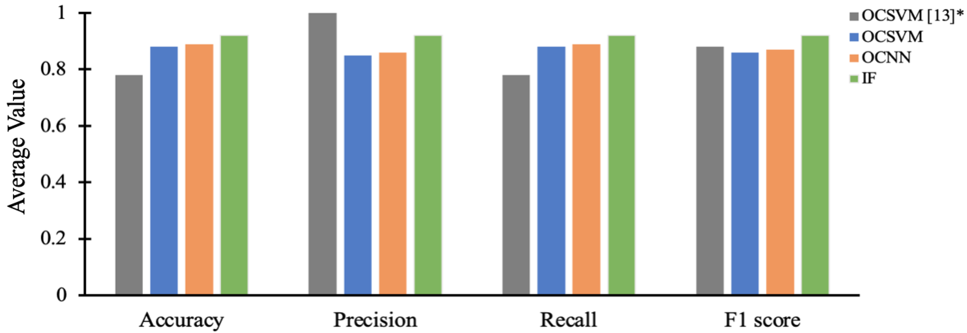
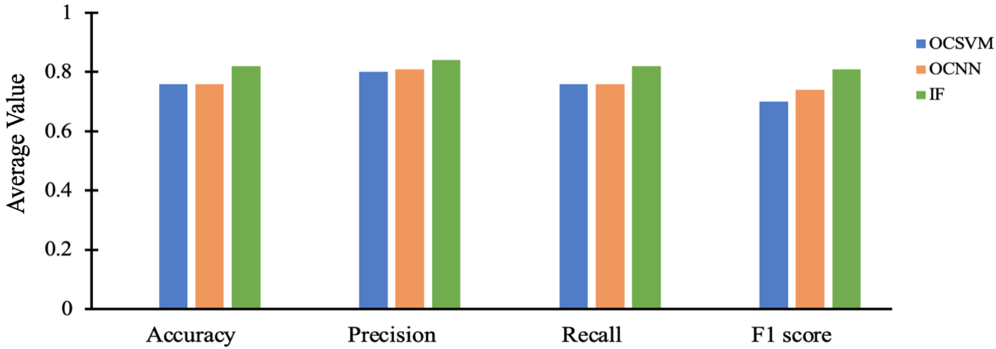
  • Conduct comparative performance analysis between OCSVM, OCNN, and IF based on their decision scores instead of using traditional binary predictions and employing analysis of variance (ANOVA) and Tukey’s range test for confirming validity of results;
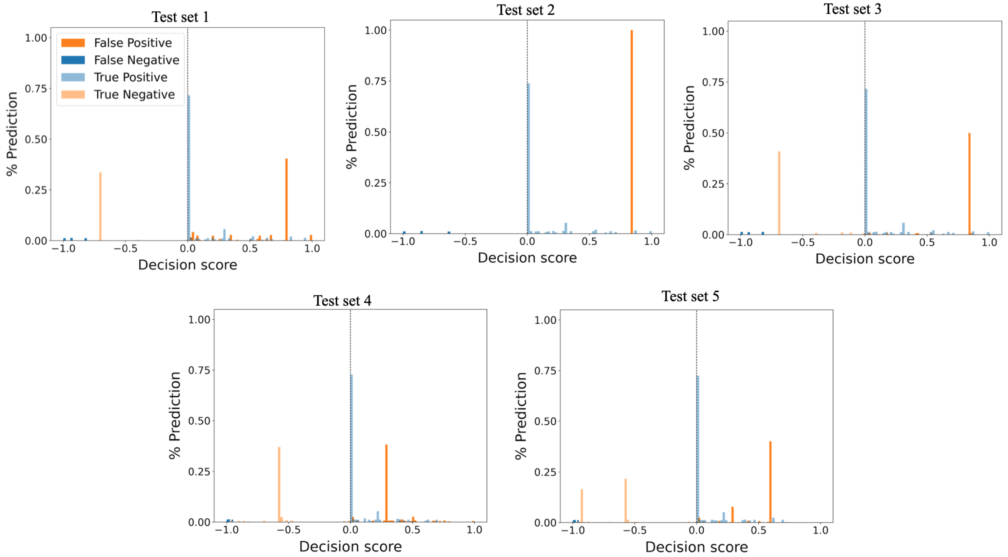
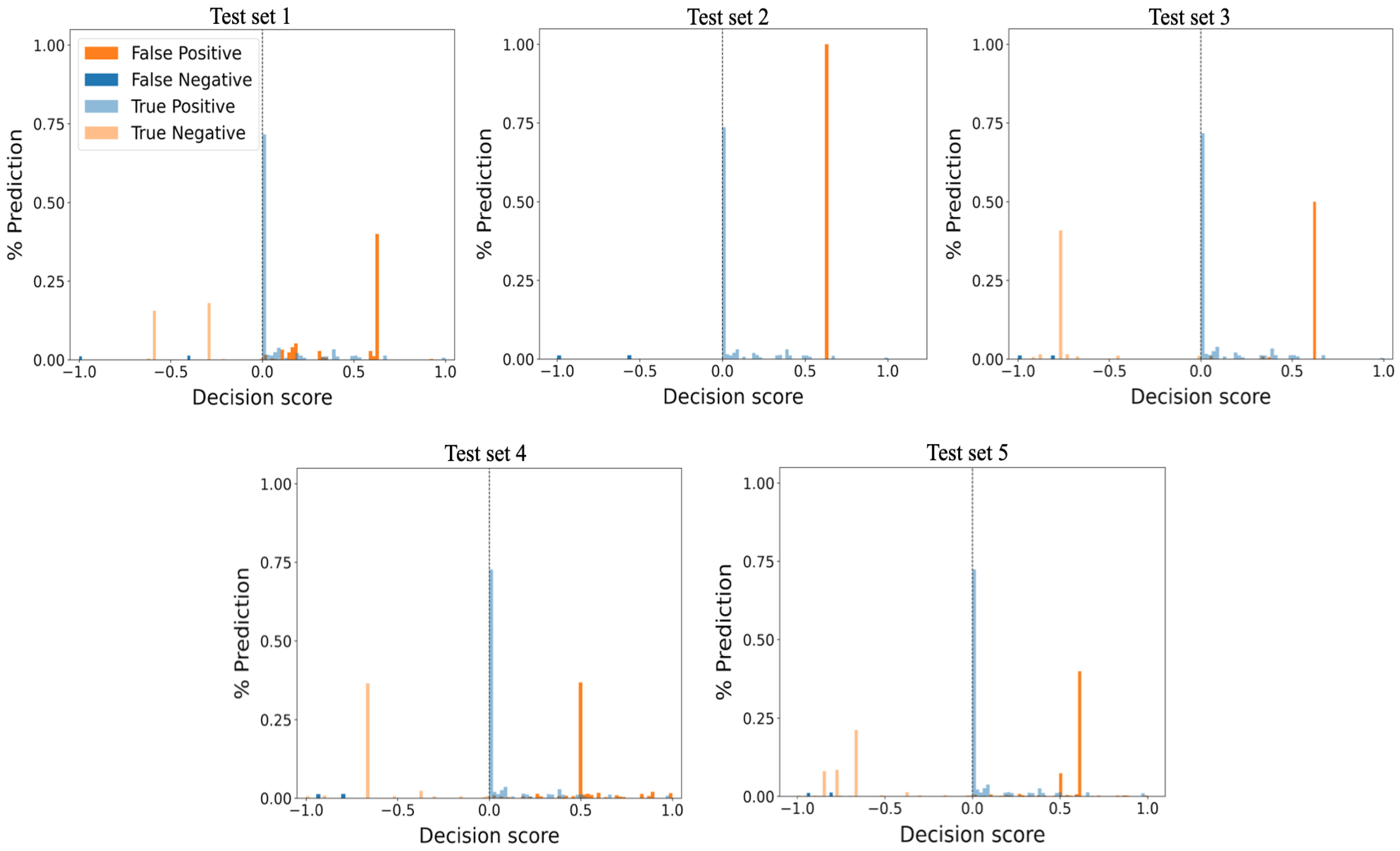
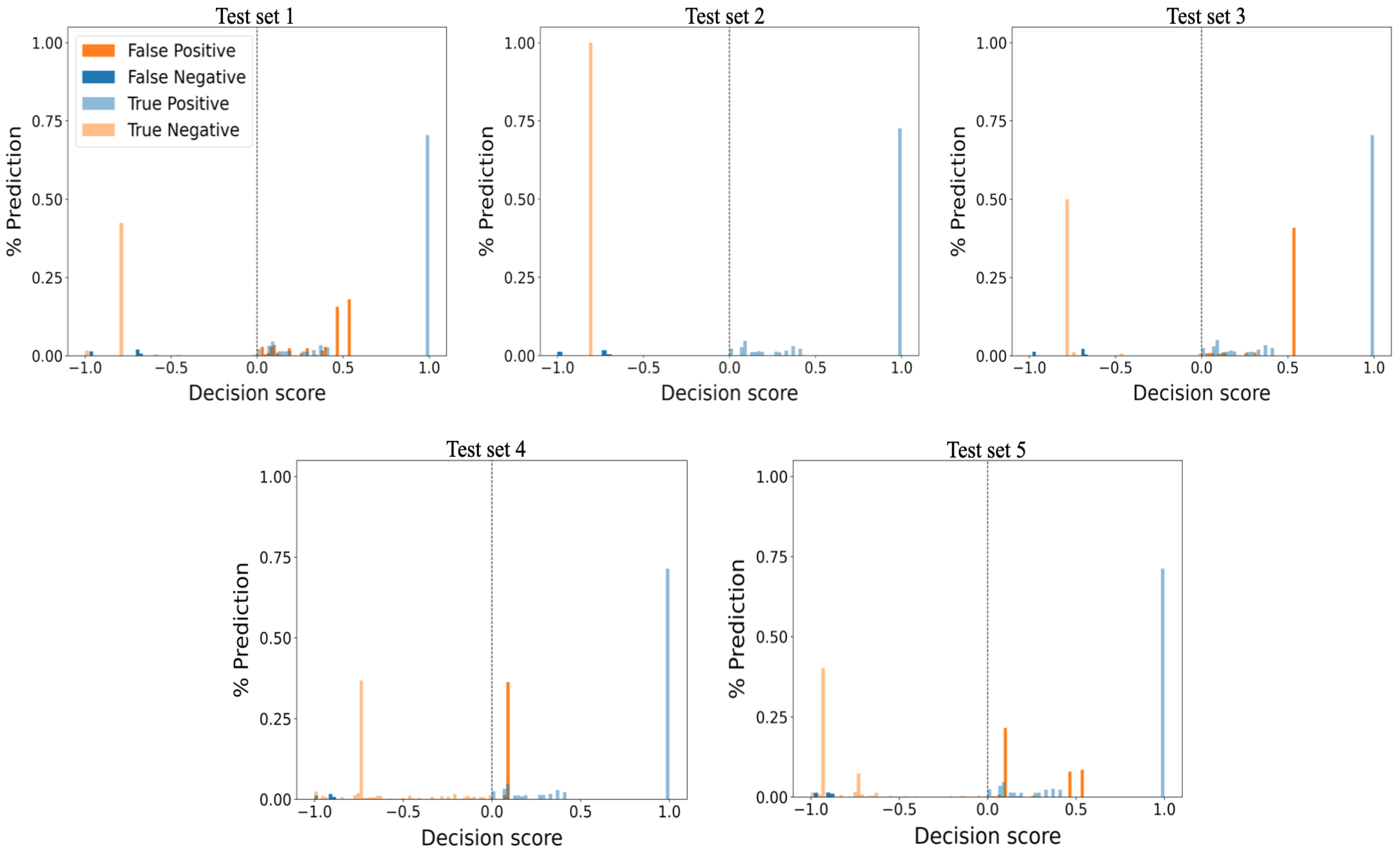
  • Introduce a new histogram-based approach for visualizing anomaly-detection algorithm performance and prediction confidence.

1.2. Outline of the Paper

This paper is organized as follows. Section 2 presents a detailed overview of the related works, followed by Section 3, which discusses the details of the experimental setup and the approach to collecting data for training and evaluating the ML algorithms. Section 4 discusses the proposed unsupervised anomaly detection frameworks, and after that, Section 5 presents the results and analysis. Finally, Section 6 concludes the paper and provides recommendations for future work.

2. Related Work

Inoue et al. employed unsupervised ML algorithms for anomaly detection in water treatment systems [20]. They compared two unsupervised methods: a deep neural network consisting of feed-forward layers with multiple inputs and outputs and a one-class support vector machine (OCSVM). The authors claimed that the deep neural network model generated fewer false positives than the OCSVM, although the OCSVM could detect more anomalies. The authors report recall values less than 0.7 for both deep neural network and OCSVM.
Tomlin et al. [21] proposed a clustering approach for network intrusion-detection system implementation in ICS. Their experimental results highlighted the issues associated with using cluster analysis as a unique tool for anomaly-based intrusion detection. Although the work of Tomlin et al. seems promising, it focused on mainly simulated experimental data, which sometimes fail to represent an actual ICS setup.
Xiao et al. [22] proposed a noninvasive power-based anomaly-detection scheme for detecting attacks on PLCs using long short-term memory. Their work detected malicious software execution in a PLC by analyzing the PLC power consumption. Xiao et al. achieved accuracy as high as 99%. However, PLC power consumption is affected by power supply instability and electronics malfunction, and can produce false-positive values.
In [23], the authors used a fully connected neural network and an autoencoder to detect anomalies in network traffic. Their results demonstrated a higher detection rate and lowered false positive rate when compared with eight other modern anomaly detection techniques. Potluri et al. [24] also employed Artificial Neural Networks (ANN) for identifying false data injection attacks in ICS. The classification report obtained in [24] shows a promising detection accuracy with ANN.
In [25], Elnor et al. proposed a semisupervised dual isolation forest-based anomaly detection approach using the normal process operation data of the secure water treatment (SWaT) testbed and water distribution testbed. They compared their approach to other anomaly detection techniques for ICS in terms of precision, recall, and F1-score. They achieved a 7% improvement in the F1-score and detected 19 out of 36 SWaT attacks.
Ahmed et al. [26] proposed an unsupervised learning approach using isolation forest to detect covert data integrity assault on a smart grid communication network. Although they achieved an average accuracy of 93%, their approach focused on simulated experimental data and may not represent ICS accurately. From the aforementioned, it can be realized that isolation forest is a tremendous unsupervised learning approach with high performance in anomaly detection. However, there are not enough applications of isolation forest techniques for anomaly detection in PLCs and ICSs.
Liu et al. [27] proposed an anomaly detector based on subspace technique and quantization method for amplitude-frequency characteristic deviation of ICSs. Their approach is practical and may be readily deployed in real ICS. However, the work does not address ICS confidentiality attack. Reported results show an inability to detect anomalies in ICSs with aggressive disturbances and instabilities. The work in [27] highlights the general challenges associated with deploying anomaly detection models in resource-constrained embedded devices for ICS protection.
PLC protection has some challenges associated with applying anomaly detection techniques [27,28,29,30]. Most legacy PLCs in ICSs have insufficient low-level documentation making it challenging to perform forensic investigations in cases of cyber-attacks or anomalous events [31]. Security mechanisms and forensic tools dedicated for PLCs to perform comprehensive security investigations are lacking [32]. Lastly, PLC availability in an ICS environment is often paramount. Therefore, shutting down a PLC-based ICS for forensic investigations is often not feasible [28]. Therefore, robust detection techniques are required for real-time anomaly detection in PLCs and ICSs.
An unsupervised ML technique called OCSVM was employed to detect anomalies in PLCs successfully in [13]. Their experiment simulated a traffic light control system using a PLC. They captured relevant PLC memory addresses into a log file for real-time data recording from the traffic light operation. The captured data was normalized and used for training the OCSVM model. Training and test accuracies were 98% and 82%, respectively. However, OCSVM recall values on some test cases were as low as 75%, and the average accuracy over their three-test cases was 78%. The low-performance metrics of detection technique in [13] call for the need to investigate robust detection techniques for anomaly detection in PLCs.
While OCSVM has been used as an effective unsupervised technique for anomaly detection, OCSVM performance is unsatisfactory on complex, high-dimensional datasets [33,34]. A one-class neural network (OCNN) with a one-class objective function was used for anomaly detection in complex datasets [33]. Despite its great potential on complex datasets, OCNN has not been applied to ICS or PLC for anomaly detection purposes. This work examines OCSVM, OCNN, and IF ML techniques for detecting PLC anomalous behavior by tracking the operations at the PLC input and output memory addresses.

3. Experiment Setup

This section provides the details of the experimental setup used in this work to implement the traffic light system. The ICS used in this work is patterned after the one described in [13,15].

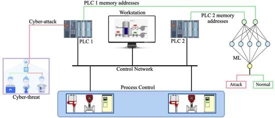
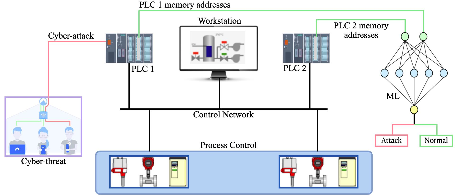
3.1. Description of Control Setup

Siemens’s open-source traffic light control program [15] was used to implement a traffic light system to control vehicles and pedestrian traffic at a pedestrian crossing with red, yellow, and green signals. In addition to the traffic light signals, each pedestrian light was equipped with a pushbutton for pedestrians to request green light signals. The following safety requirements were taken into account in the control logic program in order to prevent any hazard to pedestrians or drivers:
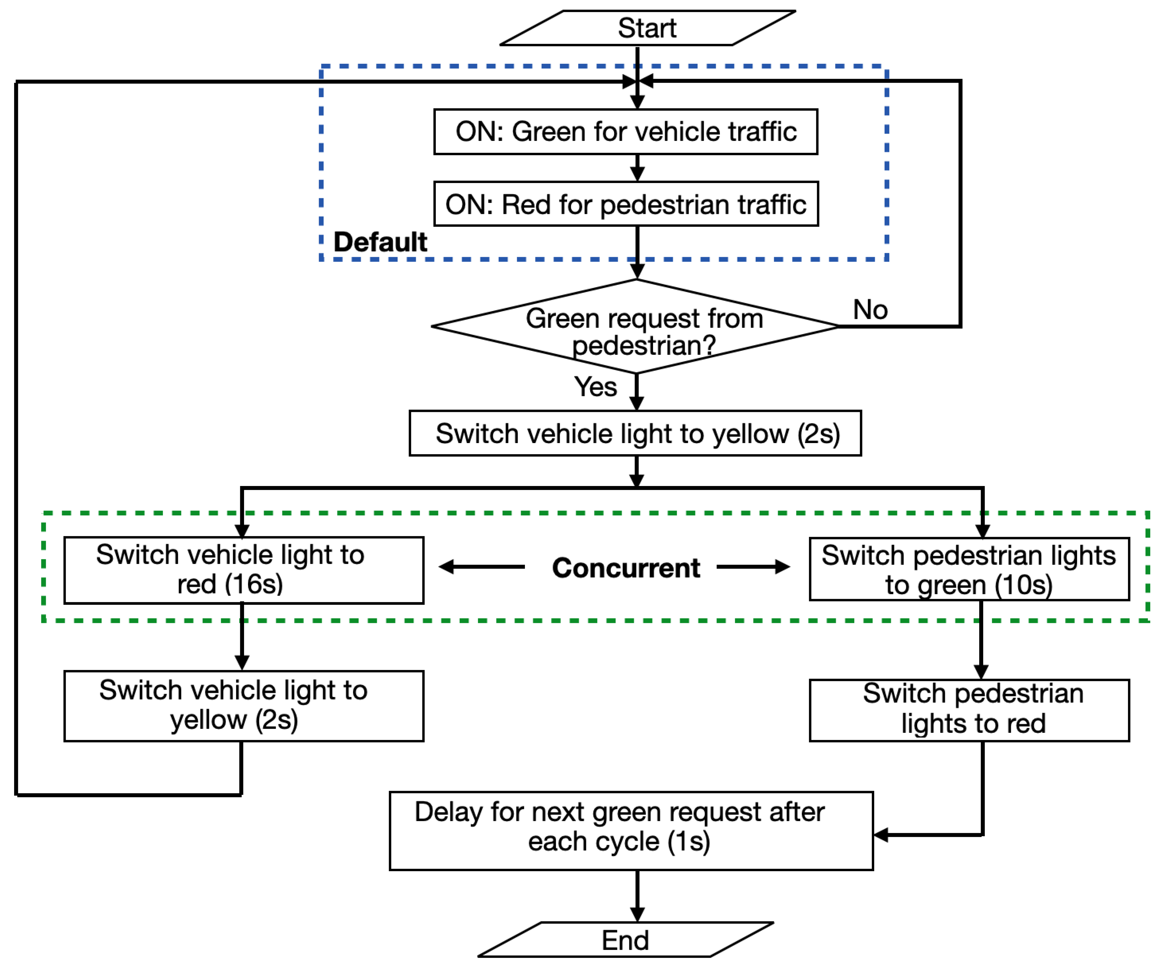
  • The control system default operation should turn ON the green and red light signals for the vehicle traffic and pedestrian traffic, respectively, to define a safe starting point;
  • Whenever the program receives a green request from the pedestrian through the pushbutton, the vehicle traffic light signals must change from green to red via yellow.
Apart from the safety requirements, Figure 2 summarizes the control setup operation. In [13,15], a system was constructed using Siemens S&-1212C PLC loaded with the TLIGHT control program. This work implements the TLIGHT control logic using OpenPLC [35] and ScadaBR [36]. Figure 3 provides a block diagram of the experimental setup for recording training and test data. The experimental setup’s main components are described below.

3.2. OpenPLC

OpenPLC is an open-source simulation environment for home and industrial automation systems development [35]. OpenPLC runtime is versatile, and it creates a virtual PLC architecture on supported hardware to mimic PLC behavior. OpenPLC supports several firm PLC devices [37,38,39] and personal computers (PC) running Linux and Windows operating systems to create flexible soft PLCs installations [35]. The TLIGHT system [15] was implemented in two parts in OpenPLC. The first part was the control program development similar to the description of Figure 2 in ladder logic form in OpenPLC editor. OpenPLC editor was used to simulate and test the TLIGHT system logic to ensure that the program was error-free and accurately represented the TLIGHT system description in [13,15]. The simulated program followed the IEC 61131-3 standard for PLC programs [40]. The ladder logic implementation is publicly available on [41]. Finally, the ladder logic was converted to a structured text format that can be run and interpreted by the OpenPLC runtime.
The soft PLC in Figure 3 was implemented with a PC running Linux version of OpenPLC. The experimental setup in this paper will work on all OpenPLC supported hardware devices [35,37,38,39]. The second part of the implementation was the program’s deployment in structured text format onto the OpenPLC runtime for real-time program execution. PLC consists of a central processing unit (CPU), memory areas (also referred to as address space in OpenPLC), and input/output devices. Internally, the program works by continuously scanning the program for every 100 ms. Each scan cycle consists of three crucial steps: check inputs, execute program logic, and update outputs. The cyclical PLC runtime process continues so long as the runtime is set to running mode as described in Algorithm 1.
Algorithm 1: PLC runtime execution.
Jcp 02 00012 i001

3.3. Human Machine Interface (HMI)

ScadaBR [36], an open-source supervisory control and data acquisition (SCADA) system, was utilized as the HMI to monitor and control the PLC runtime. ScadaBR depicts the control system’s state in real-time. It allows direct observation and execution of control commands to PLC. The PLC input and output memory addresses were mapped to corresponding Modbus input and output addresses in the HMI. At the end of every HMI cycle time (100 ms), ScadaBR records available data at the input and output Modbus addresses to a log file. Finally, TLIGHT system operations are exported from the HMI as CSV file for preprocessing and training of the detection models. The HMI application also operates independently of the PLC, as described in Algorithm 2.
Algorithm 2: HMI application execution.
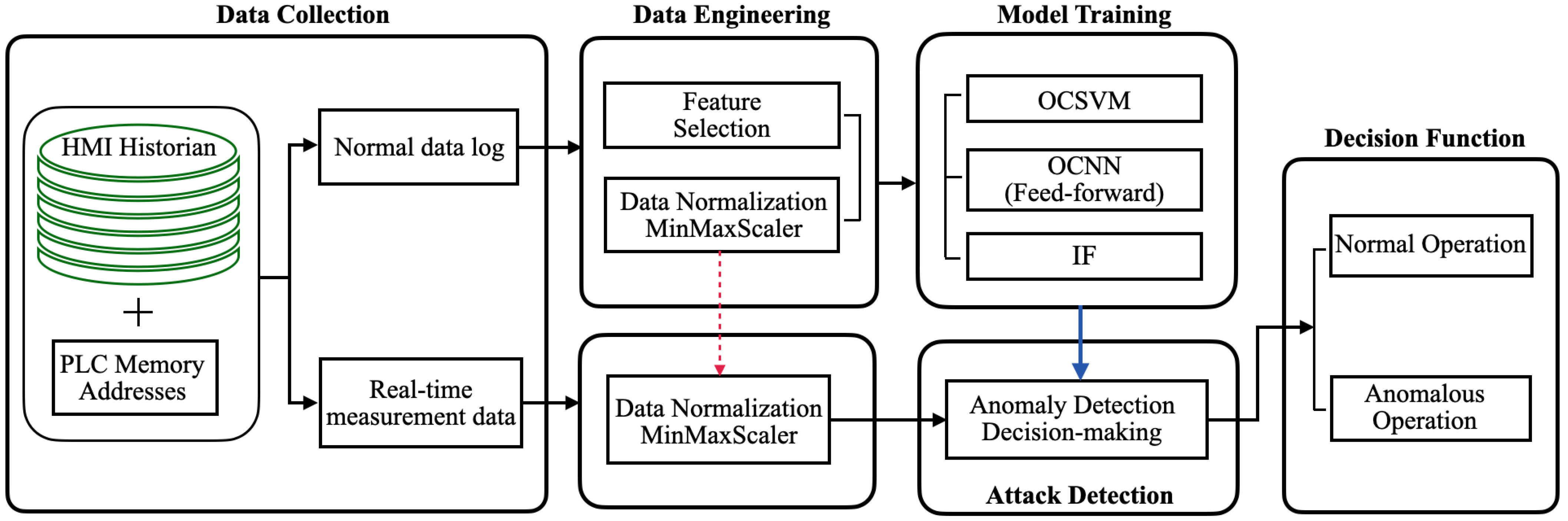
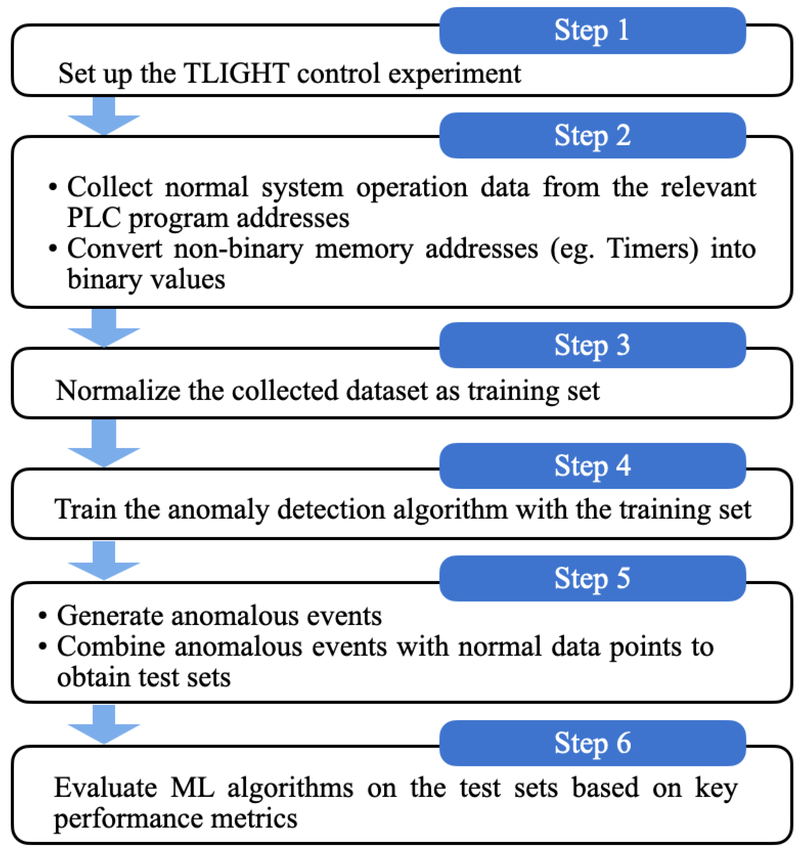
Jcp 02 00012 i002

4. Proposed Method

The proposed anomaly detection systems described here use the normal process data from TLIGHT system’s input and output signals. Details about the data collection, anomalies, and theoretical background of the algorithms used in the proposed methods are described in this section. Figure 4 is a framework of the anomaly detection approach that shows how the proposed methods could be implemented in other real-world ICS scenarios. The process starts with offline training of OCSVM, OCNN, and IF using the dataset from HMI historian directly recorded from the PLC memory addresses. Training data consists of relevant features which are normalized to retain the minimum and maximum features values. The processed data are used to develop the detection models. The trained models are serialized onto a separate computer for real-time PLC anomaly detection. During testing or online detection, real-time measurement data is obtained from the HMI historian, and information about the training data normalization procedure is used to process the online data - indicated by the red dotted arrows in Figure 4. The final decision is made by each trained detection model for specified time frames.

4.1. Data Collection and Preprocessing

ML relies heavily on data by using statistical models and algorithms to build models capable of predicting outcomes for a given input [42]. As a result, data quality is critical to ML model robustness. Data is collected from the HMI historian. The HMI monitors and records the memory addresses with timestamps via the Modbus communication protocol. The data is recorded for about 4 days to ensure enough training and test data to evaluate the proposed techniques in this work. In order to ensure a fair comparison between this work and [13], the approach described here follows a similar approach in [13] as closely as possible. Figure 5 summarizes the approach to the data collection and preprocessing.

4.1.1. Anomalous Scenarios

In order to evaluate and compare the performance of the different anomaly-detection techniques proposed in this work, five different test sets are generated. Each set contains normal and anomalous TLIGHT system events. Anomalous system events for the five test sets are derived from seven scenarios. All seven attack scenarios could generally represent real-world scenarios resulting from malfunctioning sensors and actuators, such as broken connectors, damaged cable insulation, physical obstruction, or natural disasters. It is crucial to quickly identify the anomalies in all scenarios because they could indicate hardware failure mode or the need for system maintenance. Furthermore, each scenario can also represent a specific malicious attack on an ICS. The seven attack scenarios are outlined below.
  • Anomalous scenario 1: All the vehicles and pedestrians’ green lights are turned ON at the same time. The purpose of this anomalous event is to violate the TLIGHT system safety rules. This attack generally represents a real-world scenario in which an attacker has compromised the PLC operations through elevation of privileges attack with the aim of causing traffic collision between vehicles and pedestrians.
  • Anomalous scenario 2: All the traffic lights are shut down. This attack aims to simulate an unnecessary traffic scenario for the vehicles and deny pedestrians’ green light requests. This attack represents a real-world scenario in which an attacker has introduced logic bomb attack inside the PLC ladder logic with the aim of terminating TLIGHT system operations.
  • Anomalous scenario 3: All pedestrians and vehicles’ traffic light signals are turned ON. This attack scenario aims to violate the TLIGHT system safety requirements. This attack generally represents a real-world scenario in which an attacker has compromised the wired connection between the PLC and physical components with the aim of causing a denial-of-service attack. This attack could lead to traffic jams and delays.
  • Anomalous scenario 4: Refuse all green light requests from the pedestrians. This attack scenario violates the TLIGHT system logic and operation cycle. This attack generally represents a real-world scenario in which an attacker tampered with the HMI communication protocol due to unencrypted communication with the aim of causing a denial-of-service attack.
  • Anomalous scenario 5: All vehicles and pedestrians’ red light signals are turned ON at the same time. The motive of this attack is to cause unnecessary traffic for both vehicles and pedestrians and violate the TLIGHT system’s default setting. This attack generally represents a real-world scenario in which an attacker has introduced a hardware trojan inside the physical components causing the red light signals to respond differently from the PLC logic.
  • Anomalous scenario 6: The vehicle’s yellow signals timing bits are manipulated. This kind of anomaly is stealthy and subtle because all the traffic lights seem to be operating normally with manipulated timing bits. This attack generally represents a real-world scenario where an attacker has executed a man-in-the-middle attack by spoofing the vehicle and pedestrian timing bits signals.
  • Anomalous scenario 7: Delay timing bits for subsequent pedestrian green requests, and pedestrians’ green light phase duration are manipulated. This attack scenario is similar to attack scenario six in its subtlety and difficulty of detection from a human perspective. This attack generally represents a real-world scenario in which an attacker has executed a man-in-the-middle attack by spoofing the delay timing bits for pedestrian green request signals.

4.1.2. Test Cases

The details of the five test cases considered in this study are:
  • Test set 1 contains 5000 normal and anomalous events samples, of which 10 % are anomalous instances. The 10 % of anomalous instances consists of 10 % anomalous scenarios 1, 2, 3, 4, and 5;
  • Test set 2 contains 7000 test samples, of which 10 % are anomalous events. These anomalous events consist solely of anomalous scenario 3;
  • Test set 3 contains 13,130 normal and anomalous samples. About 20 % of the data contains anomalous instances sampled from anomalous scenarios 1 and 3. Anomalous scenarios 1 and 3 consist of 50 % each of the total anomalous events in test set 3;
  • Test set 4 contains 15,000 test samples of which anomalous instances in the test sample are 30 % . These anomalous instances are sampled from anomalous scenarios 6 and 7. Moreover, anomalous scenarios 6 and 7 consist of 20 % and 10 % anomalies, respectively. This particular test set comprises only timing bits anomalies;
  • Test set 5 is the most diverse and complicated test set. Test set 5 contains 18,270 normal and anomalous test samples. A total of 50 % of the test data is anomalous instances sampled from anomalous scenarios 1, 2, 3, 5, 6, and 7. This test set is the only set with a mixture of timing bits anomalies and traffic light signals anomalies. It is also the test set with the highest number of anomalies. Anomalous scenario 1 comprises 5 % of the test data, scenario 2 is 10 % , scenario 3 is 10 % , scenario 5 is 5 % , scenario 6 is 5 % , and anomalous scenario 7 is 15 % of the test data.
The total training dataset samples and test sets 1-3 are consistent with the number of samples used in [13]. Test set 4 and 5 consist mainly of timing bits anomalies. Table 1 summarizes the number of records and proportion of anomalies in the training and test sets.

4.2. OCSVM-Based Detection Approach

Scholkopf et al. [43] proposed OCSVM, a maximum-based classifier established on support vector machines. The OCSVM is an unsupervised anomaly-detection algorithm that learns a decision function for separating the normal class from the anomalies [44]. Given a training dataset { X i | i = 1 , 2 , 3 , n } where X i R d , the OCSVM separates the data points from the origin in the feature space by a hyperplane and maximizes the distance from the hyperplane to the origin. OCSVM finds a decision function f F that separates the data points into positive and negative scores. The positive scores represent the region in the feature space where X i F , and F is the set that carries a high concentration of the data points, also known as the minimum-volume set. The negative scores represent all other data points or anomalies. High dimensional Hilbert space H, can be used to transform each data point X i via a feature map Φ : R d H generated by a positive-definite kernel, k ( X , X ) . The optimization problem for separating the data from the origin in the OCSVM is therefore given by
min w , b 1 2 w 2 C N n = 1 N ξ b s . t : w , Φ ( X i ) b ξ i , i , ξ i 0 , i
where b is the variable that controls the algorithm’s bias. The optimization problem is formulated such that w · ϕ ( X ) b is positive for as many N training examples as possible. The C value is a hyperparameter that serves as the differential weight of the normal data points compared to the anomalous data points. The value, ν = 1 / C is regarded as the prior probability that a data point in the training set is an anomaly, thereby regulating the trade-off between false positives and false negatives in the model. The slack variable ξ allows some data points in a nonseparable dataset to be within the margin. As a result, for the given data X, the decision function f F ( X n : ) is
f F ( X n : ) = w T Φ ( X n : ) b
The function definition in (2) is responsible for separating the data points from the origin by determining whether a point is in the positive or negative set. The width of the margin is controlled by b [ 0 , 1 ] and w is the normal vector of the hyperplane. The input data is projected into a nonlinear high-dimensional space by Φ ( X n : ) , and the slack variable ξ models the separation errors in the same way as the feature space of (1). Therefore, the overall OCSVM objective function is
min w , b 1 2 w 2 + 1 ν N n = 1 N max ( 0 , b w , Φ ( X n : ) ) b
While the literature reports different variations of OCSVM, this work presents an OCSVM model that is developed by using the same model parameters in [13] to serve as a baseline upon which our proposed methods could be compared. OCSVM model learning process is controlled by using hyperparameters. Table 2 shows the hyperparameters for the OCSVM. According to [13], the modeling parameters in Table 2 were selected as optimal hyper-parameters for the OCSVM algorithm after investigating various hyperparameter ranges.

4.3. OCNN-Based Detection Approach

Neural networks for one-class classification have been proposed in [45,46,47]. However, this work presents OCNN algorithm formulated on the foundation of OCSVM optimization problem [43], and a proposed alternating minimization algorithm in [33] to form a feed-forward neural network architecture capable of detecting PLC anomalies. OCNN combines the ability of feed-forward neural network to extract features from the data along with a one-class objective to become a universal anomaly detector. Given a feed-forward neural network with a hidden layer, activation function g, and an output node, the alternate minimization algorithm proposed by [33] is used to obtain the objective function. Derivation of the OCNN follows the overall OCSVM objective function in (3). The resulting objective function is used to solve the scalar output obtained from the hidden layer to the output layer w, and the weight matrix from the input to the hidden node V as
arg min w , V 1 2 w 2 + V 2 2 + 1 ν N n = 1 N ( y n , y ^ ( w , V ) )
where
( y , y ^ ) = max ( 0 , y y ^ ) , y n = b , and y ^ ( w , V ) = w , g ( V X n )
Using the same alternate minimization approach as [33], the optimization problem for the bias, b is
arg min b 1 ν N n = 1 N max ( 0 , b y ^ ) b
Finally, the OCNN objective function generalization is
min w , b , V 1 2 w 2 + 1 2 V 2 1 ν N n = 1 N max 0 , b w , g ( V X n : ) b
where ν parameter controls the trade-off between maximizing the distance of the hyperplane from the origin and the number of data points allowed to cross the hyperplane. This approach allows the model to utilize rich features obtained from unsupervised transfer learning, particularly for anomaly detection in a complex dataset where the decision boundary between the normal data points is highly nonlinear. The solution to optimizing (4) is summarized in Algorithm 3.    
Algorithm 3: OCNN Algorithm.
Jcp 02 00012 i003
Given a training dataset { X i | i = 1 , 2 , 3 . . . , n } , the width b of the hyperplane margin is first initialized. The model uses backpropagation to learn the neural network parameters ( w , V ) . The model then iteratively updates b to achieve convergence. Then, the scoring function S n labels the data points as normal and anomalous instances based on the convergence criterion ϵ with:
y = 1 if S n ( x ) > ϵ 1 if S n ( x ) ϵ
where y represents binary classes of the decision function scores, S n ( x ) .
The OCNN architecture consisted of 32 hidden layers with rectified linear activation (ReLU) function. Various hyperparameters are used to configure the OCNN model. Table 3 shows the optimal hyperparameters chosen for the OCNN after hyperparameter tuning.

4.4. Isolation Forest-Based Detection Approach

Isolation forest (IF) is an unsupervised learning technique that builds binary trees ensemble for a given dataset for anomaly detection [48,49,50] IF assumes that anomalies make up the minority of a given dataset. As a result, anomalies have attribute values that are different from the normal instances. IF uses several isolation trees and trains each tree on a subset of the training dataset. IF uses the following parameters for constructing the binary trees:
  • Total number of isolation trees ( n t ) ;
  • Sample size of training data subset used to train each isolation tree ( n m a x ) ;
  • Maximum number of features representing a subset of the data features used to train each tree ( f m a x ) .
Algorithm 4 summarizes the IF algorithm training process. During training, IF recursively partitions the training data with an axis-parallel cut at randomly chosen partition points in randomly selected attributes. Next, IF isolates the partitioned instances into nodes with fewer and fewer instances until the points are isolated into singleton nodes containing one instance [48]. IF randomly selects attributes splits q and a split subset p within a specified range, resulting in a left ( X l ) and right ( X r ) subsets of the data each time until all training samples are isolated into singleton nodes. Algorithm 5 summarizes the recursive binary splitting concept for separating anomalies by IF.
Algorithm 4: Train I F ( X , n t , n m a x , f m a x ) .
Jcp 02 00012 i004
Algorithm 5 shows that after each split, isolation tree ( i T r e e ) produces a node which is either an internal node ( i n N o d e ) or external node ( e x N o d e ) depending on whether there is a further possibility of splitting the former into subsequent split regions. Consequently, the two internal node subsets ( X l and X r ) are split further until they reach an external node. External nodes are considered as leaves of branches when the maximum tree depth is reached or the last nodes in branches when the data subset size of the region is one.
Algorithm 5: Train i T r e e ( X ) .
Jcp 02 00012 i005
Anomalous events are considerably different from the normal data points, and so the smaller paths in the isolation tree construction correspond to the lower dimensionality of the subspaces in which the anomalies have been isolated. IF works under the implicit assumption that it is more likely to isolate subspaces of lower dimensionality created by random splits [48]. The decision score S n ( x ) for a given data sample x based on a detection threshold ϵ is given by
S n ( x ) = 2 h ¯ ( x ) H
where H is the average expected path length of trees with anomalies considered as 1 while normal instances are labeled as 1 as follows
H = 2 ln f m a x 1 + 1.2 2 f m a x 1 f
The average path length on all trees h ¯ ( x ) can be derived as
h ¯ ( x ) = 1 n t n = 1 n t h i ( x )
where h i ( x ) is the n t h tree path length established by the number of edges in the tree. The IF algorithm is developed into a model using optimized hyperparameters. Table 4 shows the IF model’s optimal hyperparameters after tuning a range of hyper-parameters.

5. Results and Discussions

The evaluation is based on performance metrics, results from predictions on the test data, and comparison with previous work trained on a similar dataset. The dataset is an HMI historian log of operations at PLC memory addresses publicly available at [41]. Data of PLC memory addresses operations are obtained through the Modbus communication protocol between the PLC and HMI. Google’s Tensorflow [51], an open-source deep neural network library, is used for training the OCNN model and subsequently serialized onto a separate computer for online TLIGHT system anomaly detection. Evaluation results and performance metrics calculations are performed by using the Scikit-learn library [52].

5.1. Performance Metrics

The performance metrics of the detection models in identifying anomalies in the TLIGHT dataset are derived from the confusion matrix. Totally, four evaluation outcomes are generated by the confusion matrix: true positive (TN), true negative (TN), false positive (FP), and false negative (FN). These outcomes are used for calculating the accuracy, precision, recall, and F1-score of anomaly detection models.
Accuracy measures the proportion of correct predictions on the test data given by
Accuracy = TP + TN Real positives + Real negatives
Precision is a measure of the proportion of predicted positives that are true positives. Precision is defined as
Precision = TP TP + FP
Recall measures the proportion of actual positives that are correctly classified. It represents the ability of the model to detect all positive samples. Recall is
Recall = TP TP + FN
The F1-score is the harmonic mean of precision and recall. F1-score has its best value of 1, indicating perfect precision and recall, and its worst value of 0. It is defined as
F 1 - score = 2 × precision × recall precision + recall

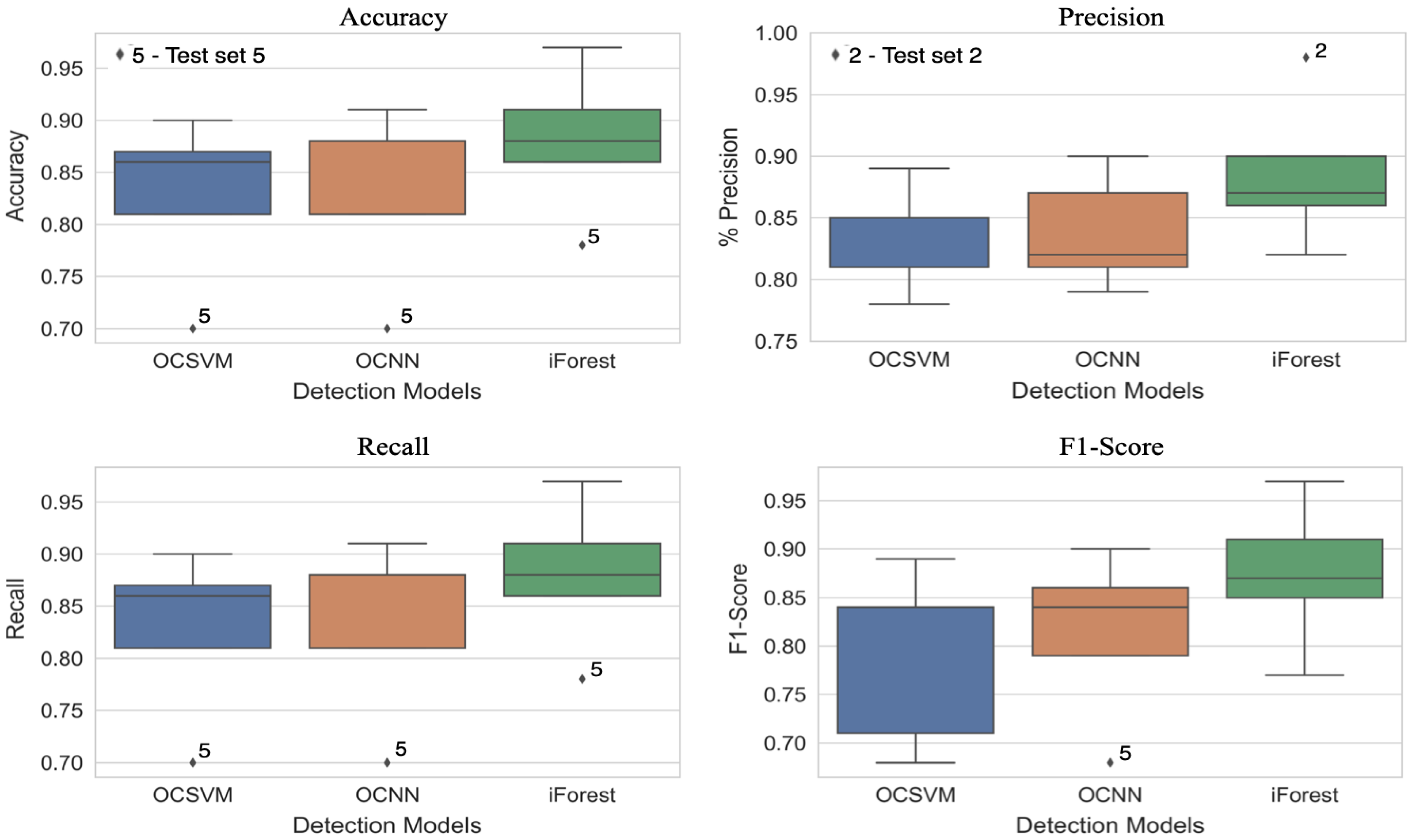
5.2. Performance Evaluation

This work presents a new way of visualizing anomaly detection algorithm results using a histogram. Although histograms have been used in previous work to present detection algorithms results [53,54,55,56], the approach presented in this work is new and provides a better understanding of detection algorithms performance by revealing the exact proportions of true positives, true negatives, false positives, and false negatives of detection algorithms.
Visualization of results is done by first separating the decision scores (real numbers) into positive and negative scores represented by P 1 and N 1 respectively. Next, decision scores are separated into true positives, true negatives, false positives, and false negatives with associated notations x t p , x t n , x f p , and x f n , respectively, based on the ground truth of the test sets. Different algorithms provide different decision scores based on their objective functions, so the resulting x t p and x f p scores are normalized to a range between 0 and 1 using the maximum and minimum values in P 1 . In contrast, x t n and x f n scores are normalized to range between 0 and 1 using the maximum and minimum values in N 1 . Furthermore, to ensure an objective comparison of the different algorithms, the x t p and x f n quantities are normalized as a function of the total ground truth positives. Similarly, x t n and x f p are normalized as a function of the ground truth negatives. Let the normalized scores of x t p , x t n , x f p , and x f n be X t p , X t n , X f p , and X f n respectively. Finally, the normalized scores are used to plot a histogram of the distribution and proportion of decision scores.
Visualization of anomaly detection results requires methods different from previous work [33], where only positive P 1 and negative N 1 scores are presented. The approach in Figure 6 reveals the fractions of P 1 , which corresponds to X t p and X f p , and the fractions of N 1 which are X t n and X f n . Moreover, the work in [33] only shows the proportions of P 1 and N 1 as a function of test data size on the histogram’s y-axis, which makes it challenging to visualize the N 1 scores, primarily because test sets in anomaly detection mainly have smaller negative class proportions [45]. On the contrary, the proposed approach normalizes the histogram frequency (y-axis) to a range of 0 to 100 % to present a better relative decision scores visualization. The visualization described here normalizes the x and y axes for easier comparison of different detection algorithms’ performance. Finally, the proposed visualization approach may be applied to supervised ML algorithms for binary classification.

5.2.1. Performance of OCSVM

OCSVM’s recall values on test sets 1, 2, 3, 4, and 5 are 90 % , 87 % , 86 % , 81 % , and 70 % , respectively. Figure 6 illustrates the benefits of the proposed visualization as it reveals OCSVM’s overall behavior on all test sets. A similar distribution of TP scores is observed on all test sets, showing how OCSVM learned the TLIGHT system’s normal behavior during training process. OCSVM found detecting normal traffic transitions involving vehicles’ green light signals challenging, leading to high TP scores that lie along the decision boundaries in all test cases. Again, FN scores of test sets 1 and 3 involve the same data records being misclassified as anomalies. Moreover, FN scores of test sets 4 and 5 represent identical normal data records misclassified as anomalies. The aforementioned show the importance of the proposed visualization in this work as Figure 6 reveals OCSVM’s true performance on each data record, which would not be possible with the traditional histogram approach [33].
Although OCSVM’s recall values decrease steadily from test sets 1 to 5, the normalized true positive scores are low in all test cases. In all test cases, OCSVM misclassifies over 30 % anomalous instances as normal instances leading to high levels of FP in all test cases. In addition, Figure 6 shows that in all test cases in which OCSVM makes an accurate positive class (normal) prediction, the score (levels of confidence) of predictions are low and lie along the decision boundary. Although OCSVM detects several positive classes, it has a greater chance of misclassifying normal data points as anomalies because of the low confidence of the positive class prediction. Moreover, about 75 % of correct positive class predictions occur close to the decisions boundary with low prediction confidence. The low prediction confidence makes OCSVM unstable for TLIGHT system anomaly detection. Figure 6 shows a histogram of normalized FP, FN, TP, and TN decision scores made by OCSVM on test sets 1–5.
OCSVM learns the TLIGHT system’s normal behavior during training with a 100 % precision and 98 % F1-score. The results substantiate the procedure this work adopts in conducting the experiment and recording data as it is similar to the training results in [13]. Overall, OCSVM performs best on test set 1. OCSVM performance on test sets 2 and 3 are similar with an F1-score of 84 % . OCSVM has its least performance on test sets 4 and 5, with F1-scores of 71 % and 68 % respectively. OCSVM model is unable to detect over 20 % of anomalies in test sets 4 and 5 because of the large proportion of anomalies consisting of timing bits anomalies. Therefore, OCSVM appears to be ineffective at detecting TLIGHT system errors consisting of system timing bits manipulation. Table 5 summarizes the performance of the OCSVM described here and the OCSVM in [13]. Table 5 shows that the OCSVM reported here and in [13] have similar training performance due to the datasets and underlying TLIGHT experiment being designed identically. Test sets 1–3 in this work are created to be the same size as the test sets in [13]; however, the exact nature and distributions of errors in [13] are unknown and may be the reason for the slight differences seen in the Table 5.

5.2.2. Performance of OCNN

OCNN’s performance on all metrics is similar to OCSVM. OCNN’s recall value on test set 1 is high at 91 % , whereas the recall values on test sets 2 and 3 are similar at 88 % . A closer observation of Figure 7 reveals that in all test sets, TP prediction scores by OCNN are close to the decision boundary signifying low confidence of the positive class prediction. Over all test cases, about 75 % of the correctly predicted positive class have scores closer to the decision boundary, which shows that OCNN has potential instabilities similar to OCSVM. In addition, OCNN misclassifies more than 25 % of anomalies as normal instances, which is undesirable, especially in ICS anomaly detection. However, the TN and FP scores in all test sets are high, showing OCNN’s robustness in detecting outliers. OCNN misclassifies several anomalies as normal instances, especially in test sets 2–5, leading to high false positive rates. Figure 7 shows a histogram of normalized FP, FN, TP, and TN decision scores made by OCNN on test sets 1–5.
OCNN has good performance on all metrics on test sets 1, 2, and 3, similar to OCSVM. OCNN learns the TLIGHT system’s normal behavior well by having a training recall of 97 % . However, OCNN’s performance on test sets 4 and 5 is low with F1-scores of 79 % and 68 % respectively. Table 6 shows OCNN’s ability to detect changes in the light signals behavior of the TLIGHT system and an inability to detect timing bits errors. OCSVM and OCNN have similar performance because the OCNN objective function is developed as an improvement upon the OCSVM optimization problem in Equation (3). Table 6 summarizes OCNN’s performance on the five test sets.

5.2.3. Performance of Isolation Forest

Unlike OCSVM and OCNN, IF uses tree ensembles to isolate anomalies from the dataset instead of learning the system’s normal behavior. IF achieves high recall rates on test sets 1 and 2 at 91 % and 97 % , respectively. IF misclassifies about 40 % of anomalies as normal instances in test set 3, which resulted in a reduced recall rate of 88 % . In test set 2, IF classifies normal and anomalous data points almost perfectly with high confidence, thereby achieving a precision of 98 % . Unlike OCSVM and OCNN, IF’s decision scores on TN and TP are consistently high, which means that whenever IF correctly predicts a normal instance, it is certain about the detection decision. In addition, Figure 8 shows that for more than 25 % of the time, whenever IF correctly detects anomalous instances, the associated decision scores are high, signifying high detection confidence. Figure 8 shows that IF’s decision scores are far away from the decision boundary, which makes IF a stable model for detecting anomalies in the TLIGHT system. IF decision scores are confident, therefore, it is an attractive approach for ICS anomaly detection. Figure 8 shows a histogram of normalized FP, FN, TP, and TN decision scores made by IF on test sets 1–5.
Similar to OCSVM and OCNN, IF has an outstanding training performance. IF has an excellent performance on test sets 1 and 2 on all evaluation metrics. IF performance on test sets 3 and 4 are similar at an average recall value of 87 % , whereas it has its lowest performance on test set 5. Test sets 4 and 5 consist of timing bits anomalies, and IF achieves recall rates of 86 % and 82 % , respectively. Results indicate that IF can detect timing bits errors better than OCSVM and OCNN. Table 7 shows a summary of evaluation results for IF.

5.3. Statistical Hypothesis Test

Statistical evidence about the best-performing detection model proposed in this work is conducted using Analysis of Variance Test and Tukey’s range test. F1-score is selected as the evaluation metric in the hypothesis test because F1-score is a great measure of the trade-off between precision and recall, especially for imbalanced datasets.

5.3.1. Analysis of Variance Test (ANOVA)

ANOVA is a statistical model used to determine if a significant difference between the means of two or more data sets exists [57,58]. One-way ANOVA is chosen because of the interest in examining one independent variable’s influence, which is F1-score. First, OSCVM, OCNN, and IF performances are evaluated on 20 different test samples of the exact sizes as test sets 1, 2, 3, 4, and 5. Next, each detection algorithm’s F1-score is computed on 20 different samples of each test set. The assumptions about the data set are
  • data points in each test sample are independent and identically distributed; and
  • data points are normally distributed.
In addition, the hypotheses for the statistical test are
  • null hypothesis ( H 0 ) : The mean F1-score of all detection algorithms are equal; and
  • alternate hypothesis ( H a ) : One or more of the mean F1-score are unequal.
Based on the one-way ANOVA test, the F value is 14.972, and a p-value < 0.001 is achieved. One-way ANOVA shows significant evidence to reject the null hypothesis. Rejecting the null hypothesis indicates a considerable difference between at least two detection algorithms at a confidence level above 95 % . Although one-way ANOVA reveals a difference in the three algorithms’ performance, statistically, it is not clear which specific algorithm performs best or worst. Therefore, a post hoc analysis is required to identify the best-performing algorithm.

5.3.2. Tukey’s Range Test

Tukey’s range test is a statistical test used as post hoc analysis after one-way ANOVA [59]. Tukey’s range test compares all possible mean F1-score pairs for all detection algorithms and precisely identifies differences between the pairs greater than the expected standard error. Tukey’s range test is based on the same assumptions as ANOVA. Table 8 depicts Tukey’s range test results at α = 0.05 .
The mean F1-score for IF significantly differs from OCNN; hence IF outperforms OCNN. However, the mean F1-score difference between OCNN and OCSVM is insignificant; therefore, OCNN and OCSVM perform at par. Lastly, Tukey’s range test indicates sufficient statistical evidence to reject the null hypothesis between the group IF-OCSVM and conclude that IF outperforms OCSVM. Results in Table 8 indicate that IF is the superior detection model for the TLIGHT dataset, whereas OCNN and OCSVM have similar overall performance.

5.4. Summary of Results

The overall performance of the detection algorithms is summarized in this section. Figure 9 shows box plots of OCSVM, OCNN, and IF results distributions with the outlier test case labeled where applicable. IF has the highest median accuracy of 88 % . Furthermore, accuracy and recall box plots in Figure 9 show that all methods have outlier performance more than 1.5 times the interquartile value on test set 5. However, the precision box plot of Figure 9 indicates that IF’s precision value of 98 % on test set 2 is an outlier. The precision box plot shows no outliers for OCSVM and OCNN. Lastly, the F1-score box plot in Figure 9 shows that the only F1-score outlier is OCNN’s result on test set 5 and the F1-scores distribution of IF is right-skewed. Therefore, the overall results indicate that all the detection models find it challenging to detect anomalies in test set 5. Nevertheless, all the detection models have similar performance distributions on test sets 1–4.
It is insightful to compare the detection models’ average performance with the reported results in [13] on all evaluation across test sets 1–3: IF performs about 5 % better than OCSVM, OCNN, and [13] in accuracy, precision, and recall. However, in terms of F1-score, IF averages about 7 % over OCSVM, OCNN, and [13]. In all evaluation metrics, OCNN and OCSVM perform similarly. Figure 10 shows the comparison between the detection models in this work and the reported results in [13]. Test sets 1–3 in this work are created to be the same sizes as the test sets in [13]; however, the exact nature of anomalies and their relative distributions in the three test sets is not provided in [13]. It is surmised that the difference in validation performance between the OCSVM in this work and the reported results of the OCSVM in [13] is due to these anomalies variations. Moreover, the reported result in [13] has a precision of 100 % in all test cases, but a low recall performance—below 83 % in all three test sets—which could potentially indicate overfitting of their model. Overall, IF achieved the best performance on all three test sets.
Test sets 4 and 5 consist of timing bits anomalies unique to this work, and such errors were not considered in [13]. Figure 11 shows the average performance comparison between OCSVM, OCNN, and IF on test sets 4 and 5. IF’s average performance is higher than that of OCNN and OCSVM on all the evaluation metrics, whereas OCNN and OCSVM perform similarly.

5.5. Practical Considerations

This work focused on TLIGHT system experiments consisting of digital signals from sensors and actuators with the purpose of monitoring operations at the PLC memory addresses. The digital nature of the experiment ensures fair comparison with previous work developed with a similar experiment. However, the work presented here need not be constrained to digital signals. The algorithms presented in this work can be extended to PLC process control involving both analog and digital signals. The proposed algorithm’s objective functions are adaptable to nonlinear scenarios; hence robust performance is expected in industrial practices involving analog control systems. The multilayer network of OCNN allows the computation of any nonlinear function [45]. OCSVM and IF have been employed to successfully detect PLC anomalies involving analog signals in [20,25,60].
The presented techniques are general methods that can be implemented in real-world ICS infrastructure with minimum effort. The outstanding performance of the proposed techniques can be realized on legacy and embedded PLCs. An approach may be to compile the trained models to C code using open-source compilers such as [61,62,63], which, as an example, support x86 and ARM64 processor architectures. The generated C code should be readily portable to dedicated ARM and general-purpose processors [64] for real-time inference. A similar approach to the experiment conducted in this work may also be employed. The trained models may be serialized onto a separate PC with a data pipeline to the HMI historian and PLC memory addresses to receive data and perform real-time anomaly detection.

5.6. Limitations

While this work makes significant contributions to the scientific body of ICS anomaly detection, there are some limitations to the proposed approaches. The proposed histogram-based visualization approach is limited to anomaly-detection algorithms with signed output results. A detection algorithm’s output must be positive and negative real numbers representing normal and anomalous points or vice-versa in order for the proposed visualization approach to be effective. The histogram-based visualization plots reveal that OCSVM and OCNN make less-confident predictions. OCSVM and OCNN have similar decision scores distributions across all five test sets because they are both formulated from a similar optimization problem. Observing OCSVM and OCNN performance limitations may not have been possible without the proposed visualization approach. Furthermore, comparing anomaly-detection algorithms performances based on decision scores instead of traditional binary predictions requires decision scores normalization. Since different anomaly detectors might produce decision scores on different scales, decision scores normalization is required for fair comparison.
In addition, there are some limitations associated with the proposed techniques. OCSVM is sensitive to the choice of kernels, and ν parameters [45], hence OCSVM is not robust in ICS applications without a deeper understanding of the ICS. OCSVM limitation can partially be solved by using variable subsampling [65] during model training in the context of ICS with unpredictable behavior. The feed-forward nature of the neural network in OCNN makes the algorithm sensitive to noise [45]. Therefore, clean ICS data should be used for OCNN training to avoid model overfitting. Finally, IF algorithm’s recursive data partitioning could lead to lower performance in high-dimensional ICS data due to the masking effect of locally noisy and irrelevant features. As a result, feature-selection techniques [66,67] should be employed in high-dimensional ICS data before IF model training.
Although IF has a stellar performance on key evaluation metrics on test sets 1–3, it achieved lower recall values on test sets 4–5, which contain timing bits error. Some anomalous data points are detected by either OCSVM or OCNN, but IF fails to detect them. This shows that the proposed algorithms have strengths and weaknesses on different subsets of the data, and hence, a single detection algorithm may not be able to generalize to an arbitrary ICS setup. However, aggregating the predictions from individual anomaly detection models could potentially result in a robust model capable of detecting anomalies in an arbitrary ICS setup.

6. Conclusions

This work presents unsupervised ML algorithms for anomaly detection, including cyber-attacks on PLCs and ICS. A previously studied TLIGHT ICS system was used. The control system’s normal behavior is recorded through the PLC memory addresses. One-class support vector machine, one-class neural network, and isolation forest algorithms were developed using system process data. This work proposes a new histogram-based visualization technique for demonstrating true positives, true negatives, false positives, and false negatives proportions in anomaly detection models’ performance. The proposed visualization technique can also be extended to supervised ML algorithms involving binary classification. Results indicate that OCSVM and OCNN have similar performance on all evaluation metrics, which are inferior to IF performance. A hypothesis test is conducted using one-way ANOVA and Tukey’s range test to provide statistical evidence about the algorithm with the best performance. The hypothesis test indicates that IF has the best anomaly-detection rate on the TLIGHT system; however, there is insufficient statistical evidence to support any difference in performance between OCSVM and OCNN. Finally, IF achieved superior performance over results reported in prior work. The proposed techniques are generalized methods, which can be implemented in real-world ICS with minimal effort.

Recommendation

Based on the limitations outlined in this work, it is evident that some anomaly-detection algorithms will perform well on a particular subset of the dataset, whereas other algorithms will do better on other subsets of the dataset. Therefore, future work should focus on the following to address the challenge mentioned above and extend scientific knowledge:
  • improving the anomaly-detection rate on the TLIGHT system through ensemble techniques;
  • developing dual anomaly-detection algorithms that will focus on specific subsets of the dataset; and
  • extending the proposed techniques in this work to other publicly available anomaly detection datasets.

Author Contributions

Conceptualization, E.A.B. and J.W.B.; software, E.A.B.; validation, E.A.B. and J.W.B.; investigation, E.A.B.; resources, J.W.B.; writing—original draft preparation, E.A.B.; writing—review and editing, E.A.B. and J.W.B. All authors have read and agreed to the published version of the manuscript.

Funding

This research was funded, in part, by the State of Tennessee and the Tennessee Technological University Center for Manufacturing Research.

Institutional Review Board Statement

Not applicable.

Acknowledgments

The views expressed in this paper are those of the authors, and do not reflect the official policy or position of the state of Tennessee and Tennessee Technological University.

Conflicts of Interest

The authors declare no conflict of interest.

References

  1. Kello, L. The Virtual Weapon and International Order; Yale University Press: New Haven, CT, USA, 2019. [Google Scholar]
  2. Yaacoub, J.P.A.; Salman, O.; Noura, H.N.; Kaaniche, N.; Chehab, A.; Malli, M. Cyber-physical systems security: Limitations, issues and future trends. Microprocess. Microsyst. 2020, 77, 103201. [Google Scholar] [CrossRef] [PubMed]
  3. Thakur, K.; Ali, M.L.; Jiang, N.; Qiu, M. Impact of cyber-attacks on critical infrastructure. In Proceedings of the 2016 IEEE 2nd International Conference on Big Data Security on Cloud (BigDataSecurity), IEEE International Conference on High Performance and Smart Computing (HPSC), and IEEE International Conference on Intelligent Data and Security (IDS), New York, NY, USA, 9–10 April 2016; pp. 183–186. [Google Scholar]
  4. Plėta, T.; Tvaronavičienė, M.; Casa, S.D.; Agafonov, K. Cyber-attacks to critical energy infrastructure and management issues: Overview of selected cases. Insights Into Reg. Dev. 2020, 2, 703–715. [Google Scholar] [CrossRef]
  5. Wardak, H.; Zhioua, S.; Almulhem, A. PLC access control: A security analysis. In Proceedings of the 2016 World Congress on Industrial Control Systems Security (WCICSS), London, UK, 12–14 December 2016; pp. 1–6. [Google Scholar]
  6. Abbasi, A.; Holz, T.; Zambon, E.; Etalle, S. ECFI: Asynchronous control flow integrity for programmable logic controllers. In Proceedings of the 33rd Annual Computer Security Applications Conference, Orlando, FL, USA, 4–8 December 2017; pp. 437–448. [Google Scholar]
  7. Abbasi, A. Ghost in the PLC: Stealth on-the-fly manipulation of programmable logic controllers’ I/O. In Proceedings of the Black Hat EU, London, UK, 1–4 November 2016; pp. 1–4. [Google Scholar]
  8. Yau, K.; Chow, K.P. PLC forensics based on control program logic change detection. J. Digit. Forensics, Secur. Law 2015, 10, 5. [Google Scholar] [CrossRef] [Green Version]
  9. Langmann, R.; Stiller, M. The PLC as a smart service in industry 4.0 production systems. Appl. Sci. 2019, 9, 3815. [Google Scholar] [CrossRef] [Green Version]
  10. Tsiknas, K.; Taketzis, D.; Demertzis, K.; Skianis, C. Cyber Threats to Industrial IoT: A Survey on Attacks and Countermeasures. IoT 2021, 2, 163–188. [Google Scholar] [CrossRef]
  11. Spyridopoulos, T.; Tryfonas, T.; May, J. Incident Analysis & Digital Forensics in SCADA and Industrial Control Systems. In Proceedings of the 8th IET International System Safety Conference Incorporating the Cyber Security Conference, Cardiff, UK, 16–17 October 2013. [Google Scholar]
  12. Boeckl, K.; Boeckl, K.; Fagan, M.; Fisher, W.; Lefkovitz, N.; Megas, K.N.; Nadeau, E.; O’Rourke, D.G.; Piccarreta, B.; Scarfone, K. Considerations for Managing Internet of Things (IoT) Cybersecurity and Privacy Risks; US Department of Commerce, National Institute of Standards and Technology: Gaithersburg, MD, USA, 2019.
  13. Yau, K.; Chow, K.P.; Yiu, S.M.; Chan, C.F. Detecting anomalous behavior of PLC using semi-supervised machine learning. In Proceedings of the 2017 IEEE Conference on Communications and Network Security (CNS), Las Vegas, NV, USA, 9–11 October 2017; pp. 580–585. [Google Scholar]
  14. Aboah, B.E.; Bruce, J.W. Anomaly Detection for Industrial Control Systems Based on Neural Networks with One-Class Objective Function. Proc. Stud. Res. Creat. Inq. Day 2021, 5, 86. [Google Scholar]
  15. Siemens, S. S7-300 Programmable Controller Quick Start, Primer, Preface; Technical Report; C79000-G7076-C500-01; Siemens: Nuremberg, Germany, 1996. [Google Scholar]
  16. Chen, Y.; Wu, W. Application of one-class support vector machine to quickly identify multivariate anomalies from geochemical exploration data. Geochem. Explor. Environ. Anal. 2017, 17, 231–238. [Google Scholar] [CrossRef]
  17. Welborn, T. One-Class Support Vector Machines Approach for Trust-Aware Recommendation Systems; Shareok: Norman, OK, USA, 2021. [Google Scholar]
  18. Hiranai, K.; Kuramoto, A.; Seo, A. Detection of Anomalies in Working Posture during Obstacle Avoidance Tasks using One-Class Support Vector Machine. J. Jpn. Ind. Manag. Assoc. 2021, 72, 125–133. [Google Scholar]
  19. Ahmad, I.; Shahabuddin, S.; Malik, H.; Harjula, E.; Leppänen, T.; Loven, L.; Anttonen, A.; Sodhro, A.H.; Alam, M.M.; Juntti, M.; et al. Machine learning meets communication networks: Current trends and future challenges. IEEE Access 2020, 8, 223418–223460. [Google Scholar] [CrossRef]
  20. Inoue, J.; Yamagata, Y.; Chen, Y.; Poskitt, C.M.; Sun, J. Anomaly detection for a water treatment system using unsupervised machine learning. In Proceedings of the 2017 IEEE International Conference on Data Mining Workshops (ICDMW), New Orleans, LA, USA, 18–21 November 2017; pp. 1058–1065. [Google Scholar]
  21. Tomlin, L.; Farnam, M.R.; Pan, S. A clustering approach to industrial network intrusion detection. In Proceedings of the 2016 Information Security Research and Education (INSuRE) Conference (INSuRECon-16), Charleston, SC, USA, 30 September 2016. [Google Scholar]
  22. Xiao, Y.j.; Xu, W.y.; Jia, Z.h.; Ma, Z.r.; Qi, D.l. NIPAD: A non-invasive power-based anomaly detection scheme for programmable logic controllers. Front. Inf. Technol. Electron. Eng. 2017, 18, 519–534. [Google Scholar] [CrossRef]
  23. Muna, A.H.; Moustafa, N.; Sitnikova, E. Identification of malicious activities in industrial internet of things based on deep learning models. J. Inf. Secur. Appl. 2018, 41, 1–11. [Google Scholar]
  24. Potluri, S.; Diedrich, C.; Sangala, G.K.R. Identifying false data injection attacks in industrial control systems using artificial neural networks. In Proceedings of the 2017 22nd IEEE International Conference on Emerging Technologies and Factory Automation (ETFA), Limassol, Cyprus, 12–15 September 2017; pp. 1–8. [Google Scholar]
  25. Elnour, M.; Meskin, N.; Khan, K.; Jain, R. A dual-isolation-forests-based attack detection framework for industrial control systems. IEEE Access 2020, 8, 36639–36651. [Google Scholar] [CrossRef]
  26. Ahmed, S.; Lee, Y.; Hyun, S.H.; Koo, I. Unsupervised machine learning-based detection of covert data integrity assault in smart grid networks utilizing isolation forest. IEEE Trans. Inf. Forensics Secur. 2019, 14, 2765–2777. [Google Scholar] [CrossRef]
  27. Liu, B.; Chen, J.; Hu, Y. Mode division-based anomaly detection against integrity and availability attacks in industrial cyber-physical systems. Comput. Ind. 2022, 137, 103609. [Google Scholar] [CrossRef]
  28. Ahmed, C.M.; MR, G.R.; Mathur, A.P. Challenges in machine learning based approaches for real-time anomaly detection in industrial control systems. In Proceedings of the 6th ACM on Cyber-Physical System Security Workshop, Taipei, Taiwan, 6 October 2020; pp. 23–29. [Google Scholar]
  29. Priyanga, S.; Gauthama Raman, M.; Jagtap, S.S.; Aswin, N.; Kirthivasan, K.; Shankar Sriram, V. An improved rough set theory based feature selection approach for intrusion detection in SCADA systems. J. Intell. Fuzzy Syst. 2019, 36, 3993–4003. [Google Scholar] [CrossRef]
  30. Raman, M.G.; Somu, N.; Mathur, A.P. Anomaly detection in critical infrastructure using probabilistic neural network. In International Conference on Applications and Techniques in Information Security; Springer: Berlin/Heidelberg, Germany, 2019; pp. 129–141. [Google Scholar]
  31. Benkraouda, H.; Chakkantakath, M.A.; Keliris, A.; Maniatakos, M. Snifu: Secure network interception for firmware updates in legacy plcs. In Proceedings of the 2020 IEEE 38th VLSI Test Symposium (VTS), San Diego, CA, USA, 5–8 April 2020; pp. 1–6. [Google Scholar]
  32. Wu, T.; Nurse, J.R. Exploring the use of PLC debugging tools for digital forensic investigations on SCADA systems. J. Digit. Forensics, Secur. Law 2015, 10, 7. [Google Scholar] [CrossRef] [Green Version]
  33. Chalapathy, R.; Menon, A.K.; Chawla, S. Anomaly detection using one-class neural networks. arXiv 2018, arXiv:1802.06360. [Google Scholar]
  34. Bengio, Y.; LeCun, Y. Scaling learning algorithms towards AI. Large-Scale Kernel Mach. 2007, 34, 1–41. [Google Scholar]
  35. Alves, T.R.; Buratto, M.; De Souza, F.M.; Rodrigues, T.V. OpenPLC: An open source alternative to automation. In Proceedings of the IEEE Global Humanitarian Technology Conference (GHTC 2014), San Jose, CA, USA, 10–13 October 2014; pp. 585–589. [Google Scholar]
  36. Mazurkiewicz, P. An open source SCADA application in a small automation system. Meas. Autom. Monit. 2016, 62, 199–201. [Google Scholar]
  37. Unipi Neuron Kernel Description. Available online: https://www.unipi.technology/products/unipi-neuron-3 (accessed on 3 March 2022).
  38. ZumIQ Edge Computer Kernel Description. Available online: https://www.freewave.com/products/zumiq-edge-computer/ (accessed on 3 March 2022).
  39. Automation without Limits Kernel Description. Available online: https://www.unipi.technology/ (accessed on 3 March 2022).
  40. Tiegelkamp, M.; John, K.H. IEC 61131-3: Programming Industrial Automation Systems; Springer: Berlin/Heidelberg, Germany, 2010. [Google Scholar]
  41. TLIGHT SYSTEM Source Code to TLIGHT Experiment. Available online: https://github.com/emmanuelaboah/TLIGHT-SYSTEM (accessed on 17 January 2022).
  42. Gollapudi, S. Practical Machine Learning; Packt Publishing Ltd.: Mumbai, India, 2016. [Google Scholar]
  43. Schölkopf, B.; Platt, J.C.; Shawe-Taylor, J.; Smola, A.J.; Williamson, R.C. Estimating the support of a high-dimensional distribution. Neural Comput. 2001, 13, 1443–1471. [Google Scholar] [CrossRef] [PubMed]
  44. Zhu, F.; Yang, J.; Gao, C.; Xu, S.; Ye, N.; Yin, T. A weighted one-class support vector machine. Neurocomputing 2016, 189, 1–10. [Google Scholar] [CrossRef]
  45. Aggarwal, C.C. An introduction to outlier analysis. In Outlier Analysis; Springer: Berlin/Heidelberg, Germany, 2017; pp. 1–34. [Google Scholar]
  46. Oza, P.; Patel, V.M. One-class convolutional neural network. IEEE Signal Process. Lett. 2018, 26, 277–281. [Google Scholar] [CrossRef] [Green Version]
  47. Boehm, O.; Hardoon, D.R.; Manevitz, L.M. Classifying cognitive states of brain activity via one-class neural networks with feature selection by genetic algorithms. Int. J. Mach. Learn. Cybern. 2011, 2, 125–134. [Google Scholar] [CrossRef]
  48. Liu, F.T.; Ting, K.M.; Zhou, Z.H. Isolation forest. In Proceedings of the 2008 Eighth IEEE International Conference on Data Mining, Washington, DC, USA, 15–19 December 2008; pp. 413–422. [Google Scholar]
  49. Hariri, S.; Kind, M.C.; Brunner, R.J. Extended isolation forest. IEEE Trans. Knowl. Data Eng. 2019, 33, 1479–1489. [Google Scholar] [CrossRef] [Green Version]
  50. Staerman, G.; Mozharovskyi, P.; Clémençon, S.; d’Alché Buc, F. Functional isolation forest. In Proceedings of the Asian Conference on Machine Learning, PMLR, Nagoya, Japan, 17–19 November 2019; pp. 332–347. [Google Scholar]
  51. Abadi, M.; Agarwal, A.; Barham, P.; Brevdo, E.; Chen, Z.; Citro, C.; Corrado, G.S.; Davis, A.; Dean, J.; Devin, M.; et al. TensorFlow: Large-Scale Machine Learning on Heterogeneous Systems, 2015. Available online: tensorflow.org (accessed on 17 February 2021).
  52. Pedregosa, F.; Varoquaux, G.; Gramfort, A.; Michel, V.; Thirion, B.; Grisel, O.; Blondel, M.; Prettenhofer, P.; Weiss, R.; Dubourg, V.; et al. Scikit-learn: Machine Learning in Python. J. Mach. Learn. Res. 2011, 12, 2825–2830. [Google Scholar]
  53. Goldstein, M.; Dengel, A. Histogram-based outlier score (hbos): A fast unsupervised anomaly detection algorithm. In KI-2012: Poster and Demo Track; Citeseer: Princeton, NJ, USA, 2012; pp. 59–63. [Google Scholar]
  54. Kind, A.; Stoecklin, M.P.; Dimitropoulos, X. Histogram-based traffic anomaly detection. IEEE Trans. Netw. Serv. Manag. 2009, 6, 110–121. [Google Scholar] [CrossRef]
  55. Bansod, S.D.; Nandedkar, A.V. Crowd anomaly detection and localization using histogram of magnitude and momentum. Vis. Comput. 2020, 36, 609–620. [Google Scholar] [CrossRef]
  56. Xie, M.; Hu, J.; Tian, B. Histogram-based online anomaly detection in hierarchical wireless sensor networks. In Proceedings of the 2012 IEEE 11th International Conference on Trust, Security and Privacy in Computing and Communications, Liverpool, UK, 25–27 June 2012; pp. 751–759. [Google Scholar]
  57. Goldberg, D.E.; Scheiner, S.M. ANOVA and ANCOVA: Field competition experiments. Des. Anal. Ecol. Exp. 2001, 2, 69–93. [Google Scholar]
  58. Rutherford, A. ANOVA and ANCOVA: A GLM Approach; John Wiley & Sons: Hoboken, NJ, USA, 2011. [Google Scholar]
  59. Abdi, H.; Williams, L.J. Newman-Keuls test and Tukey test. In Encyclopedia of Research Design; Sage: Thousand Oaks, CA, USA, 2010; pp. 1–11. [Google Scholar]
  60. Alqurashi, S.; Shirazi, H.; Ray, I. On the Performance of Isolation Forest and Multi Layer Perceptron for Anomaly Detection in Industrial Control Systems Networks. In Proceedings of the 2021 8th International Conference on Internet of Things: Systems, Management and Security (IOTSMS), Gandia, Spain, 6–9 December 2021; pp. 1–6. [Google Scholar]
  61. Unlu, H. Efficient neural network deployment for microcontroller. arXiv 2020, arXiv:2007.01348. [Google Scholar]
  62. XLA: Optimizing Compiler for Machine Learning. Available online: https://www.tensorflow.org/xla (accessed on 3 March 2022).
  63. NNCG: Neural Network Code Generator. Available online: https://github.com/iml130/nncg (accessed on 3 March 2022).
  64. Urbann, O.; Camphausen, S.; Moos, A.; Schwarz, I.; Kerner, S.; Otten, M. AC Code Generator for Fast Inference and Simple Deployment of Convolutional Neural Networks on Resource Constrained Systems. In Proceedings of the 2020 IEEE International IOT, Electronics and Mechatronics Conference (IEMTRONICS), Vancouver, BC, Canada, 9–12 September 2020; pp. 1–7. [Google Scholar]
  65. Aggarwal, C.C. Data Mining: The Textbook; Springer: Berlin/Heidelberg, Germany, 2015; Volume 1. [Google Scholar]
  66. Chandrashekar, G.; Sahin, F. A survey on feature selection methods. Comput. Electr. Eng. 2014, 40, 16–28. [Google Scholar] [CrossRef]
  67. Kumar, V.; Minz, S. Feature selection: A literature review. SmartCR 2014, 4, 211–229. [Google Scholar] [CrossRef]
Figure 1. A typical ICS with interconnected network configuration.
Jcp 02 00012 g001
Figure 2. Flow chart of TLIGHT system operations.
Jcp 02 00012 g002
Figure 3. Diagram of the cyber-physical system network interconnection and information flow.
Jcp 02 00012 g003
Figure 4. General framework of the anomaly detection approach.
Jcp 02 00012 g004
Figure 5. Description of the various steps involved in data collection, preprocessing, training and evaluation of the anomaly detection algorithms.
Jcp 02 00012 g005
Figure 6. OCSVM results of the normalized TP, TN, FP, and FN values on test sets 1–5.
Jcp 02 00012 g006
Figure 7. OCNN results of the normalized TP, TN, FP, and FN values on test sets 1–5.
Jcp 02 00012 g007
Figure 8. IF results of the normalized TP, TN, FP, and FN values on test sets 1–5.
Jcp 02 00012 g008
Figure 9. Box plot of OCSVM, OCNN, and IF performance distribution.
Jcp 02 00012 g009
Figure 10. Average test sets 1–3 performance of the OCSVM reported results * in [13], and the OCSVM, OCNN, and IF approaches described in this paper.
Jcp 02 00012 g010
Figure 11. Average test sets 4–5 performance of OCSVM, OCNN, and IF.
Jcp 02 00012 g011
Table 1. Number of records and proportion of anomalies in training and test data sets.
DatasetNo. of Records% Anomalies
Training set41,580n/a
Test Set 1500010
Test Set 2700010
Test Set 313,13020
Test Set 415,00030
Test Set 518,27050
Table 2. Model hyperparameters for OCSVM.
ParameterDescriptionChoice
kernelType of kernel used in the algorithmpolynomial
degreeDegree of polynomial kernel function3
coef0Controls how much the model is influenced by high-degree polynomials versus low-degree polynomials4
nu( ν )An upper bound on the fraction of training errors and a lower bound of the fraction of support vectors0.1
gammaDefines the level of a single training example’s influence0.1
Table 3. Model hyperparameters for OCNN.
Activation Function ν Learning RateNo. of Hidden Layers
ReLU0.040.000132
Table 4. Model hyperparameters for IF.
ParameterDescriptionValue
n e s t i m a t o r s Number of base estimators in the forest ensemble156
n m a x Number of training samples to draw to train each estimator180
f m a x Number of features to draw to train each estimator10
contaminationProportion of outliers in the data set0.05
Table 5. Performance of OCSVM described here and the reported results * of the OCSVM in [13].
Accuracy Precision Recall F1-Score
DatasetOCSVM[13]OCSVM[13]OCSVM[13]OCSVM[13]
Training set0.960.96 *1.001.00 *0.960.96 *0.980.98 *
Test set 10.900.78 *0.891.00 *0.900.78 *0.890.88 *
Test set 20.870.75 *0.811.00 *0.870.75 *0.840.86 *
Test set 30.860.82 *0.851.00 *0.860.82 *0.840.90 *
Test set 40.81-0.81-0.81-0.71-
Test set 50.70-0.78-0.70-0.68-
Table 6. Summary of evaluation results for OCNN.
DatasetAccuracyPrecisionRecallF1-Score
Training set0.971.000.970.99
Test set 10.910.900.910.90
Test set 20.880.810.880.84
Test set 30.880.870.880.86
Test set 40.810.820.810.79
Test set 50.700.790.700.68
Table 7. Summary of evaluation results for IF.
DatasetAccuracyPrecisionRecallF1-Score
Training set0.951.000.950.98
Test set 10.910.900.910.91
Test set 20.970.980.970.97
Test set 30.880.870.880.87
Test set 40.860.860.860.85
Test set 50.780.820.780.77
Table 8. Multiple comparison of mean F1-score for OCSVM, OCNN, and IF using Tukey’s range test at α = 0.05 .
Group 1Group 2Mean Diff.p-AdjustedReject
OCNNIF5.3200.001True
OCNNOCSVM−0.5870.862False
IFOCSVM−5.9070.001True
Publisher’s Note: MDPI stays neutral with regard to jurisdictional claims in published maps and institutional affiliations.

