Association Rule Mining Meets Regression Analysis: An Automated Approach to Unveil Systematic Biases in Decision-Making Processes

Abstract

Decisional processes are at the basis of most businesses in several application domains. However, they are often not fully transparent and can be affected by human or algorithmic biases that may lead to systematically incorrect or unfair outcomes. In this work, we propose an approach for unveiling biases in decisional processes, which leverages association rule mining for systematic hypothesis generation and regression analysis for model selection and recommendation extraction. In particular, we use rule mining to elicit candidate hypotheses of bias from the observational data of the process. From these hypotheses, we build regression models to determine the impact of variables on the process outcome. We show how the coefficient of the (selected) model can be used to extract recommendation, upon which the decision maker can operate. We evaluated our approach using both synthetic and real-life datasets in the context of discrimination discovery. The results show that our approach provides more reliable evidence compared to the one obtained using rule mining alone, and how the obtained recommendations can be used to guide analysts in the investigation of biases affecting the decisional process at hand.

1. Introduction

Decisional processes undertaken by humans are at the core of most organizations, from policy setting to IT and IT-security operations. These processes rely on cognitive resources (information, conceptual models, etc.) to help decision-makers in making appropriate decisions leading to meaningful courses of action. A prime example in the security domain is the operation of a security operation center, where technology (e.g., an SIEM—Security Information and Event Management system) supplies information to human operators who have to decide whether a specific event must be investigated [1]. The high complexity and repetitiveness of the information in input to these processes is known to lead to systematic biases in the analyst’s decision-making process [2]. How to manage these shortcomings is still an open organizational issue [3], however, the identification of the sources of these biases is a first crucial step in that direction [1]. These issues are not unique to security decisions, and extend to other application domains, such as decisions for hiring or on loans requests, which have been shown to suffer from systematic, oftentimes implicit or unknown biases [4,5].

The common underlying thread is that any process relying on human judgment must be monitored to uncover unknown and implicit biases and that can only happen by systematically reviewing decisions through objective analyses that ‘let the data speak’.

Uncovering biases from observational data is a broad and still open problem that requires a thorough exploratory analysis and understanding of the data, as well as rigorous estimations of effect sizes. The literature generally considers association rule mining for the former [6], while regression models are often used to evaluate effect sizes and rigorously evaluate evidence in the data [7]. However, when taken individually, these techniques are affected by intrinsic drawbacks. The outcome of association rule mining typically consists of several thousands of rules that cannot be easily operationalized. While a number of approaches have been proposed to prune the rule set, for instance by removing redundant rules [8] or assessing rule statistical significance [9], there is little or no support for analysts in delving deeper into the obtained outcome. Furthermore, different approaches typically lead to different outcomes, and there are no clear guidelines on how to determine the method and related parameters that best suit the data at hand, which require a deep understanding of the underlying statistical principles by the user. On the other hand, regression models are of little use without clearly defined hypotheses and a clear understanding of the data generation process.

In this work, we propose a novel methodology for uncovering systematic biases in data generating processes that combines the benefits of both worlds by leveraging principles from both association rule mining and regression analysis. We use association rule mining to extract the candidate hypotheses of biases from an exploration of data. These hypotheses are used to build regression models which provide us with statistical evidence for the presence/absence of biases in the decisional process, and effectively act as a cream-skimming mechanism to filter out hypotheses that are equivalent or that do not add significant information to uncover the data generation mechanism. This evidence can then be used by an analyst to take action and tackle the decision bias at the source.

We demonstrate our methodology in the context of discrimination detection to uncover the systematic use of sensitive data. In particular, we study the ability of the methodology to determine whether decisional processes are affected by biases that lead to unfair treatment because of personal characteristics or membership to certain (protected) societal groups. Nonetheless, our methodology is general and can be applied to the analysis of other decisional processes, e.g., for the security analysis of network traffic to uncover patterns of compromise. To evaluate the proposed methodology, we perform a set of experiments with both synthetic and real-world datasets to, respectively, validate our approach and showcase the methodology against real decision process outcomes.

This work extends our previous work [10], which only provides a high-level overview of the approach along with a proof-of-concept on a synthetic dataset. In particular, we refined the approach and extended the experimental evaluation to real-world datasets. The main contributions of this work can be summarized as follows:

• We identify general desiderata for a bias detection technique targeted at addressing sub-groups analysis;
• We propose a data-agnostic, evidence-based approach to identify well-grounded hypotheses of bias in any decisional process which aids policy makers identify potentially biased and systematic decisions affecting a group or sub-group(s) of entities of interest (e.g., sensitive subjects);
• We perform a set of experiments on synthetic data and showcase the application of our method in the domain of discrimination detection by employing two real-world datasets used in previous research on discrimination detection;
• We show that the descriptive statistics (mean, 95% confidence intervals) of the effects of interest returned by our approach can be used to further guide the policy maker in pertaining follow-up regulatory actions.

This paper is organized as follows. The next section provides background on association rule mining and regression analysis. Section 3 introduces our methodology and Section 4 presents its experimental evaluation. Section 5 provides a discussion of our method and results. Finally, Section 6 discusses related work and Section 7 provides conclusive remarks.

2. Background

We model a decision-making process as a set of records comprising a number of attributes (hereafter called variables or features) describing a given subject (e.g., a person applying for a loan) and the outcome of the process, i.e., the decision made for the subject. Intuitively, each record represents one observation of the process along with the data upon which it operated (i.e., the variables) and its outcome.

Table 1. Example decisional process of a financial institute.

	Outcome	Variables
SubjID	High Risk	Employed	Income	Gender	Ethnic Group
1	1	N	2000	M	Black
2	0	Y	10,000	F	White
⋮	⋮	⋮	⋮	⋮	⋮
100	1	N	5000	M	Asian

provides a fictional example of a decision-making process of a financial institute aiming to determine whether a given applicant should be classified as a high-risk individual, i.e., they are likely unable to refund a loan. Each record corresponds to a single loan request where SubjID provides the ID of the applicant and Employed, Income, Gender, Ethnic Group are variables characterizing the applicant. HighRisk is the binary variable describing the outcome of the process (1 encoding a ‘high-risk’ evaluation for that subject).

Decisional processes are often affected by human or algorithmic bias. In the example above, the data could reveal to an observer whether being currently employed is a relevant criterion for the bank’s decision-making process. Similarly, it could reveal how the odds of being assigned to a risk category change for every additional dollar of income. Whereas these are relations that one could reasonably expect to find in any decision process of this type, other complex dynamics can have a ‘hidden’ impact on the decision. For example, Ethnic Group may have an impact, albeit perhaps more so below certain Income levels.  A recent example of such potentially systematic biases can be found in the Netherlands; in January 2021, the national Dutch government resigned following a scandal involving unfair accusations against Dutch residents related to child benefit support. These accusations turned out to disproportionately target residents with dual nationalities and of specific ethnic origins requesting financial support for childcare from the Dutch government (https://www.theguardian.com/world/2021/jan/15/dutch-government-resigns-over-child-benefits-scandal, Last accessed 16 March 2022). Similarly, Gender or belief-related biases can interact with other variables, such as Ethnic Group or social status, to affect a decision.

To detect biases in decisional processes, one has to quantify to what extent the use of variables (e.g., Gender, Ethnic Group) has influenced the process outcome. A main challenge lies in the fact that the decisional process is often unknown. We only observe the output of a black-box process. Therefore, detecting biases in decisional processes requires reconstructing the decisional process from observational data and determining which variables were most likely used for decision making. Operationally, the problem can be formulated as deriving possible correlations between variables and the process outcome (i.e., to indicate the fact that individuals with certain attributes have higher chances of obtaining a certain outcome than individuals without those attributes).

We argue that any approach designed to tackle this challenge should meet a number of desiderata, as reported in

Table 2. Desiderata for bias detection and investigation.

Desideratum	Description and Motivations
Data agnostic	The hypothesis generation should be agnostic of the data-generation process, i.e., the (often unknown) composition of decisional processes leading to a potentially biased outcome. Ideally, an approach to uncover these latent biases should be able to determine a set of hypotheses without requiring a priori knowledge of the composition of the underlying data-generation processes; indeed, in most contexts, little or no knowledge on how the decisions are taken is available, or the decisional environment is so complex that it is impossible to know, a priori, whether the decisions in outcome will be affected by biases (latent or explicitly manifest) in the process.
No parameter tuning	The solution should not require the tuning of parameters to avoid guess-work during the setup phase, and improve the stability and interpretability of the evaluation it generates, and operate.
Feature level and Feature value level	Biases can be analyzed at different levels of granularity. Capturing biases at a feature level would allow determining which (set of) variable(s) has an impact on the outcome, i.e., whether there is a significant correlation between the type of characteristics of an individual and the outcome variable. In certain domains such as in discrimination discovery, an analyst might require a more fine-grained analysis able to identify whether individuals with certain characteristics have been treated differently. To this end, it is desirable that the outcome of the analysis highlights possible correlations between feature values and the outcome variable.
Change impact	The solution should enable the analysis of the impact of changing the value of one (or more) feature(s) on the value of the outcome, allowing the user to assess both the direction (i.e., positive or negative) and the magnitude of this impact.

.

The last three desiderata concern the capability of the approach to enable the understanding of how features and their values impact the outcome of the decisional process.

Two classes of techniques are widely used for the exploration of observational data: (i) approaches that use statistical tools, in particular regression analysis, to determine which variables are more likely able to explain the process outcome and (ii) approaches based on knowledge discovery, such as association rule mining, to measure possible differences in the proportions of positive/negative decisions on different groups of observations. We then introduce the basic concepts underlying these two lines of research and discuss their shortcomings with respect to the desiderata in Table 2.

2.1. Association Rule Mining

The goal of association rule mining is to find correlations between variables [6]. When applied to decisional processes, association rule mining aims to derive rules describing the process from observational data.

A decisional process D can be represented as a set of observations, each describing a process instance for a given subject. Given a set of variables $\mathcal{V}=\{{\mathit{Var}}_1,\dots ,{\mathit{Var}}_n\}$, each representing a characteristic of the subject, an observation t is a tuple $({\mathit{Var}}_1=v_1,\dots ,{\mathit{Var}}_n=v_n)$, where $v_i\in dom\left({\mathit{Var}}_i\right)$ is the value of variable ${\mathit{Var}}_i$ in t. Every pair ${\mathit{Var}}_i=v_i$ is called item, and a set of items itemset.

An association rule r is an implication of the form $r:X\to Y$, where X and Y are two itemsets, respectively, called antecedent and consequent of the rule. Intuitively, an association rule indicates that if X occurs in a record, then Y will also likely occur in that record. In this work, we consider class association rules [11], i.e., association rules whose consequent consists of a single class item. For the sake of simplicity, hereafter we use the term ‘rule’ to refer to a class association rule.

To assess the relevance of the mined rules, in this work, we consider two well-known and largely adopted metrics [12]: support, which represents the percentage of records in the dataset covered by a rule, and confidence, which represents the percentage of records covered by the rule among those covered by its antecedent. Formally, the support and confidence of an association rule $r:X\to Y$ with respect to a dataset D are defined as

$$\mathit{supp}\left(r\right)=\frac{\left|\right\{t\in D\mid X\cup Y\subseteq t\left\}\right|}{\left|D\right|}$$

(1)

$$\mathit{conf}\left(r\right)=\frac{\mathit{supp}\left(r\right)}{\mathit{supp}\left(X\right)}$$

(2)

It is worth noting that our approach is not constrained to the use of these metrics and other metrics could be employed to assess the relevance of the mined rules.

2.2. Regression Analysis

Regression analysis is a tool to evaluate the statistical association between at least one ‘explanatory variable’ and an ‘outcome variable’. A regression model linking the explanatory variables to the outcome variable is generally formulated on the basis of hypotheses that the analyst makes about the underlying relation. A typical regression model assumes the following general form:

$$g\left(E\left(Y\right)\right)=c+{\beta }_1{\mathit{Var}}_1+{\beta }_2{\mathit{Var}}_2+\cdots +{\beta }_n{\mathit{Var}}_n+ϵ$$

(3)

where $g(·)$ is the link function, Y is the outcome variable with mean $E\left(Y\right)$, c is the intercept, and ${\beta }_1,\cdots ,{\beta }_n$ are the regression coefficients of the n explanatory variables ${\mathit{Var}}_1,\cdots ,{\mathit{Var}}_n$, and $ϵ$ is the error term. If the analyst believes that there are interactions between explanatory variables (i.e., they have a joint effect on the dependent variable), she can capture these interactions by considering the product of the explanatory variables, denoted by ${\mathit{Var}}_i·{\mathit{Var}}_j$, as an additional explanatory variable. Equation (3) is called a regression equation; the estimation of the coefficients is the key aspect, and which link function one adopts depends on the nature of the data (e.g., a logit or a probit function for a binary outcome).

A model formulation (also called parametrization) is generally directly derived from the formulated hypotheses; however, in exploratory settings (where those hypotheses do not yet exist [7]) the model definition can generally be automated by employing techniques based on the analysis of variance (ANOVA). Again, the choice of the test to compare models depends on the type of model considered; logit models, for example, may be compared using likelihood ratio tests. to select the explanatory variables that have the highest power in ‘explaining’ the data. Given two models of the same power, the model with the fewer explanatory variables is preferred (principle of ‘minimality’). Regardless of the adopted approach to parameterize a model, it is important to verify that the chosen explanatory variables are not highly correlated, to avoid model multicollinearity that may bias the coefficient estimation. This check can be performed by calculating a correlation matrix across the variables, or a variance inflation factor (VIF) for a given model.

2.3. Limitations of Association Rule Mining and Regression Analysis

Uncovering biases from observational data requires a thorough exploratory analysis of the data, as well as rigorous estimations of effect sizes. Whereas the literature generally considers association rule mining for the former, regression models are often used to evaluate effect sizes and rigorously evaluate evidence in the data. However, both methods have intrinsic shortcomings in our application. We then discuss these shortcomings, which are summarized in

Table 3. Comparison of association rule mining and regression analysis with respect to the identified desiderata for bias detection in Table 2, where ● means “support” and ○ “no support”.

	Data-Agnostic	No Param. Tuning	Feature Level	Feature Value Level	Change Impact
Assoc. Rule Mining	●	○	○	●	○
Regression Analysis	○	●	●	●	●

.

Association Rule Mining. First, rule mining requires an analyst to carefully tune the threshold parameters for the used relevance metrics without providing a rigorous way to ‘prioritize’ rules for a certain outcome. While selecting low threshold values can lead to a large number of rules, most of which are not interesting and/or not reliable, excessively high values can easily lead to missing relevant correlations. Rule mining also lacks support for the statistical validation of the associations detected among the variables. The use of metrics such as support and confidence does not guarantee preventing the generation of false discoveries, such as rules showing dependencies likely due by chance, or rules where the antecedent contains items that are actually independent of the consequent [13]. Moreover, association rule mining only allows analysts to explore relations among single feature values and class values (feature value level analysis), while feature level analysis is not supported.

Regression analysis. Compared to association rule mining, regression analysis provides a more robust approach to statistical validation. The output provided by regression techniques supports both feature level and feature value level analysis. Moreover, they do not require the tuning of parameters. However, regression (parametric) approaches require some type of hypothesis formulation to build a model to regress on. This is desirable in general as it attaches semantic meaning to the statistical evidence found in the data. However, for data exploration tasks such as the one at hand, regression approaches are very limited in nature. Forward or backward model selection procedures [7] can be applied to identify the ‘best’ model explaining the data, but the number of models to be compared explodes exponentially as the number of allowed variable interactions increases. More importantly, there is no ‘guarantee’ that the resulting selected ‘best’ model has any useful interpretation that can be used to take action and tackle the decision bias at the source.

3. A New Approach for Bias Detection Combining Rule Mining and Regression Analysis

To detect and investigate systematic biases in decisional processes, we propose to combine principles of rule mining with regression analysis. We note that a data sanitization process should start before the application of our methodology; for example, to identify highly correlated variables in a dataset that may create multicollinearity problems biasing estimated model coefficients. When two or more highly correlated variables are present, only one should be selected for inclusion in the analysis.

Our methodology is summarized in Figure 1. First, association rule mining is employed to generate the set of relevant rules (1). For our purpose, we treat each mined rule as a candidate hypothesis for bias. In step (2), we generate regression models by considering the variables included in each selected rule and regress over them to generate the model estimates of the considered outcome variable. In step (3), a model comparison is performed to eliminate ‘redundant’ models that do not add relatively more information to the prediction than a simpler model does. This leaves us with only ‘winning’ models that, among all evaluated candidates, provide the more convincing evidence for some effect, if any. Finally, in step (4), we extract the coefficients of these selected models to identify (sub)populations of interest for which there is statistical evidence of bias in the decision making. Then, we provide a detailed breakdown of each step of the methodology.

3.1. Systematic Hypothesis Generation

Given a decisional process D, we apply class association rule mining to derive the set of relevant rules $R_{rel}$. To measure the relevance of rules, we use support and confidence, as defined in Equations (1) and (2). Specifically, we say that a rule is relevant if its support and confidence levels are above some given thresholds ${\rho }_{supp}$ and ${\rho }_{conf}$, respectively. Formally, $R_{rel}=\{r_i\mid \mathit{supp}\left(r_i\right)\ge {\rho }_{supp}\wedge \mathit{conf}\left(r_i\right)\ge {\rho }_{conf}\}$. Each rule in $R_{rel}$ is considered a candidate hypothesis of biases in the decisional process.

Example 1.

Below, we show some example (relevant) rules that can be extracted by the application of association rule mining to the decisional process of Table 1:

$$\begin{array}{cc}{r}_1:\hfill & \mathtt{Income}=5000,\mathtt{Ethnic}\mathtt{Group}=\mathit{White}\to \mathtt{HighRisk}=0\hfill \\ r_2:\hfill & \mathtt{Gender}=M\to \mathtt{HighRisk}=1\hfill \\ r_3:\hfill & \mathtt{Gender}=M,\mathtt{Employed}=N\to \mathtt{HighRisk}=1\hfill \\ r_4:\hfill & \mathtt{Income}=2000,\mathtt{Ethnic}\mathtt{Group}=\mathit{White}\to \mathtt{HighRisk}=0\hfill \end{array}$$

An analyst should investigate all the rules in $R_{rel}$ to check whether they correspond to actual biases. However, as discussed earlier, association rule mining provides very little support for this. For instance, $R_{rel}$ might contain rules that are not ‘independent’ from each other. In particular, many rules can be “subrules” of others, i.e., they extend other rules with additional itemsets as in the case of $r_2$ and $r_3$ above. Formally, a rule $r_i:X_i\to Y$ is a subrule of a rule $r_j:X_j\to Y$ if $X_i\subset X_j$. Thus, the analyst might not know whether the (possible) bias concerns the population characterized by a given rule (e.g., employed males) or whether it affects a larger population as characterized by a subrule (e.g., all males).

To find more reliable evidence of biases, in this work, we employ regression analysis to determine the statistical validity of the evidence found.

3.2. Model Derivation

To determine whether the candidate hypotheses extracted using rule mining corresponds to biases in the decisional process, we derive regression models from the set of relevant rules $R_{rel}$. Specifically, for each rule $r:{\mathit{Var}}_1=v_1,\cdots ,{\mathit{Var}}_N=v_N\to \mathtt{Class}=Y$ in $R_{rel}$, we consider the set of explanatory variables occurring in the antecedent of the rule $V_i=\{{\mathit{Var}}_1,\cdots ,{\mathit{Var}}_N\}\subseteq \mathcal{V}$ and build a corresponding regression model $M_i$ of the form of:

$$\begin{array}{c}{M}_i:\mathtt{Class}=c+\sum _{i=1}^N{\beta }_i{\mathit{Var}}_i+\sum _{1\le i<j\le N}{\beta }_{ij}{\mathit{Var}}_i·{\mathit{Var}}_j\hfill \\ \hfill \hspace{1em}\hspace{1em}\hspace{1em}\hspace{1em}\hspace{1em}+\sum _{1\le i<j<k\le N}{\beta }_{ijk}{\mathit{Var}}_i·{\mathit{Var}}_j·{\mathit{Var}}_k+\dots +{\beta }_{1\dots N}{\mathit{Var}}_1·\dots ·{\mathit{Var}}_N\end{array}$$

(4)

Example 2.

From the set of rules in Example 1, we can extract three models:

$$\begin{array}{cc}{M}_1:& \mathtt{HighRisk}=c_1+{\beta }_{1,1}\mathtt{Income}+{\beta }_{1,2}\mathtt{Ethnic}\mathtt{Group}+{\beta }_{1,3}\mathtt{Income}·\mathtt{Ethnic}\mathtt{Group}\hfill \\ M_2:& \mathtt{HighRisk}=c_2+{\beta }_{2,1}\mathtt{Gender}\hfill \\ M_3:& \mathtt{HighRisk}=c_3+{\beta }_{3,1}\mathtt{Gender}+{\beta }_{3,2}\mathtt{Employed}+{\beta }_{3,3}\mathtt{Gender}·\mathtt{Employed}\hfill \end{array}$$

Note that some rules collapse in a single model as they contain exactly the same set of variables. In our example, this is the case for rules $r_1$ and $r_4$, which are both represented by model $M_1$.

To efficiently compare the ‘credibility’ of the obtained models (next step), we organize the derived models in a hierarchical structure. To this end, we introduce a partial order relation over regression models which resembles the subrule relation. Given two regression models $M_i$ and $M_j$ defined over the sets of explanatory variables $V_i$ and $V_j$, respectively, we say that $M_j$ is nested in $M_i$, denoted as $M_j\subset M_i$, if and only if $V_i\subset V_j$. Whereas in the econometrics literature the term nested usually refers to the more general model (i.e., $M_j$ is nested in $M_i$ if $V_j\subset V_i$,), here we adopt the opposite definition to remain consistent with the definition of subrule provided in Section 3.1. Moreover, we say that $M_j$ is directly nested in $M_i$, denoted as $M_j⊏M_i$, if and only if $M_j\subset M_i$ and there does not exist a model $M_k$ such that $M_k\subset M_i$ and $M_j\subset M_k$. Based on the direct nesting relation, we construct a forest of models whereby the model at the root of each tree is the simplest model (i.e., with the smallest number of variables on the right hand side), and each child is a direct nested model of its parent(s).

Example 3.

The three models in Example 2 along with other hypothetical regression models can be represented in a hierarchy, as shown Figure 2. The hierarchy has two root nodes, i.e., $M_5$ and $M_2$, each with two children ($M_1$ and $M_4$ for $M_5$, $M_3$ and $M_4$ for $M_2$) among which one is in common (i.e., $M_4$). $M_4$ is further extended by $M_6$, which is also a child of $M_3$.

3.3. Model Comparison and Selection

Once the hierarchical structure is in place, we apply a model selection procedure by comparing each parent with all its child models. Our pruning strategy consists of checking whether the addition of variables to a child model adds information that leads to a better description of the data, or whether the simpler model is preferable (in that it describes the data indistinguishably well with respect to the more complex model). This is operationalized through the ANOVA test. Alternatives to ANOVA for model comparison exist, such as AIC, BIC, or maximum likelihood; in this work, we adopt ANOVA for model comparison, but any other method could be used. The ANOVA test is a widely used statistical test that allows one to compare the fits of two regression models, one nested in the other, by comparing the (sum of squares of the) residuals (i.e., the errors) of the respective model predictions [14].

If the output of the ANOVA test indicates that the more complex model provides a significantly better explanation of the variance in the prediction, the child model is marked as preferable compared to the more general, simpler parent model. Otherwise, the parent model is marked as preferable. Formally, given a set $\mathcal{M}$ of regression models to test, we aim to derive the set ${\mathcal{M}}_{sel}=\{M_i\in \mathcal{M}\mid \nexists M_j\in \mathcal{M}\mathrm{s}.\mathrm{t}.M_j⊏M_i\wedge \mathit{ANOVA}(M_i,M_j)\le \rho \}$, where $\rho$ represents a threshold to determine whether $\mathit{ANOVA}(M_i,M_j)$ shows a statistically significant difference in the sum of the squared residuals between the two models.

Operationally speaking, the set ${\mathcal{M}}_{sel}$ was derived using the procedure shown in Algorithm 1.

Algorithm 1: Model Selection.

This procedure takes as input (i) a model hierarchy $(\mathcal{M},⊏)$, where $\mathcal{M}$ is the set of regression models and ⊏ is the directly nested relation on $\mathcal{M}$, and (ii) a threshold $\rho$ determining whether the result of the ANOVA test is significant, and iteratively checks whether nested models provide more significant explanation of biases. At the beginning, the output set ${\mathcal{M}}_{sel}$ is initialized to the empty set, while the set of regression models to be analyzed is stored in a stack, ${\mathcal{M}}_p$, which is initialized to the root models (i.e., the models that are not nested in any other model) (lines 1–2).

The models in ${\mathcal{M}}_p$ are iteratively extracted from ${\mathcal{M}}_p$ and compared against their direct nested models using the ANOVA test (lines 4–5). Every child that is preferable compared to its parent(s) based on the ANOVA test is added to the set of winner children ${\mathcal{M}}_{wc}$ (line 5). If the set ${\mathcal{M}}_{wc}$ for a given parent $M_i$ is empty, i.e., there are no better performing children models than $M_i$ according to the ANOVA test, then $M_i$ is added to the output set ${\mathcal{M}}_{sel}$ (lines 6–7). Otherwise, the models in ${\mathcal{M}}_{wc}$ are added to ${\mathcal{M}}_p$ in order to be analyzed in the next iterations of the algorithm, i.e., they are compared against their children (line 9). The procedure terminates when ${\mathcal{M}}_p$ is empty.

Example 4.

Consider the model hierarchy in Figure 2. By applying our model selection algorithm, at the beginning, we retrieve the two parent nodes, i.e., $M_5$ and $M_2$. Supposing that the ANOVA test indicates that $M_1$, $M_3$ are the only children scoring better than $M_5$, $M_2$, respectively, $M_1$ and $M_3$ are added to the stack ${\mathcal{M}}_p$. Since $M_1$ does not have any other child, it is added to ${\mathcal{M}}_{sel}$. Instead, $M_3$ has to be compared against $M_6$. If the ANOVA test determines that $M_6$ is better than $M_3$, $M_6$ is added to ${\mathcal{M}}_p$ and, since it has no children, in the next iteration, it is added to ${\mathcal{M}}_{sel}$. At this point the procedure terminates, since there are no more models to compare, returning ${\mathcal{M}}_{sel}=\{M_1,M_6\}$.

It is worth noting that the proposed pruning procedure can theoretically lead to miss some interesting models. As the comparison only accounts for directly nested models, it is possible that models that score better than their ancestors but not than their direct parents are discarded. For example, since $M_4$ does not score better than $M_5$, it is not selected for the next iterations and, therefore, $M_6$ would have not been considered for the ANOVA test. However, it is reasonable to expect such loss to be limited. If a child model includes a variable providing a strong explanation of the observed effects, one can reasonably expect such variable(s) to have been picked up by other rules (step 1) and therefore to occur in other regression models. This leads to the otherwise discarded model being tested against different parents. This is the case, in our example, for $M_6$. While the procedure would have discarded $M_6$ if it had only $M_4$ as a parent, this model is still considered in the comparison against $M_3$ and, hence, it gets a chance to be selected.

3.4. Recommendation Extraction

The selected regression models ${\mathcal{M}}_{sel}$ obtained from step 3 provide the best ‘explanation’ of the decisional process. Each model comprises a set of coefficients $C_i=\{{\beta }_{i,1},{\beta }_{i,2},\cdots ,{\beta }_{i,k}\}$ together with an output of a statistical test determining whether each element of $C_i$ is significantly different from zero (i.e., whether the associated variable in $V_i$ is likely to have a significant effect on the outcome variable). The minimum level of statistical significance generally considered is 5% ($p\le 0.05$).

By inspecting each model $M_i\in {\mathcal{M}}_{sel}$, in this phase, we extract regressors and associated coefficients $\langle {\beta }_{i,j},{\mathit{Var}}_{i,j}=v_{i,j}\rangle$ with $p_{i,j}\le 0.05$ for which there is enough evidence to consider possible effects on the outcome variable. Each extracted pair $\langle {\beta }_{i,j},{\mathit{Var}}_{i,j}=v_{i,j}\rangle$ conveys information on the direction and size of the identified bias towards the group ${\mathit{Var}}_{i,j}=v_{i,j}$, represented, respectively, by the sign and magnitude of the coefficient ${\beta }_{i,j}$. The interpretation of this coefficient, in the case of discrete (as opposed to continuous) variables, is to be interpreted as the change in the outcome variable for observations that belong to the relevant category relative to observations in the baseline category (cf. Appendix A for a more detailed discussion).

We stress that ‘hand-picking’ variables with significant p-values is not a meaningful approach for model selection and interpretation. Differently, the goal of the proposed approach is to identify variables (possibly appearing across several selected models) for which there exists some evidence of correlation with the process outcome, and that may require additional, more rigorous investigation by an analyst or policy maker. To evaluate the strength of the emerging evidence, an analyst can, for example, compare how the associated coefficients for a variable vary across models (see analysis reported in Section 4.2 for an example), or evaluate cross-correlation effects with other variables in subsequent analyses. The output of the proposed approach serves, therefore, as an indication to guide further investigations of the data and the respective generative processes, and should not be considered as a means to automatically generate robust explanations for the data.

4. Experiments

This section discusses an application of our methodology to the problem of discrimination detection in decisional processes the Python implementation used for these experiments can be found at https://gitlab.tue.nl/lgenga/association-rule-mining-meets-regression-analysis (Last access 16 March 2022). We performed experiments with both synthetic datasets, to demonstrate the ability of our approach to detect situations in which discrimination occurred, and with real-life datasets, to evaluate the applicability of our approach to real-life scenarios. In the experiments, we assume that the policy maker knows the groups of protected subjects for which possible biases should be tested. Therefore, we only consider rules regarding these groups as initial input. This assumption is reasonable in the context of discrimination detection, where the protected groups are known a priori. Nonetheless, our approach is general and does not require a priori domain knowledge.

4.1. Approach Validation

4.1.1. Dataset and Settings

For the validation of our approach, we generated synthetic datasets to contain a known ‘amount’ of evidence of discrimination. To this end, we defined a simple decisional process regarding the hiring of candidates on the basis of their personal characteristics.

Table 4. Variables used for the generation of the synthetic dataset along with their domain.

Variables	Variable Domain
Education	Doctorate, Master, Bachelor, HighSchool
Speak Language	Y, N
Previous Role	Employee, Manager, Self-Employed, Unemployed
Country	USA, Europe, SA, China, India
Age	25–50, 50+
Class	Y, N

shows the variables characterizing the hiring process along with their domain. We consider the variable Age as a ‘discriminatory variable’, whereas the others are considered ‘context variables’. We generate the synthetic data in two steps. First, we created the discriminated groups as groups of subjects sharing the same value of Age as well as a (randomly chosen) subset of context values; the values of the other context variables were randomly assigned from the respective domains. Discriminated subjects have a probability of 80% of being assigned to class “N”. Second, we generated all ‘non-discriminated’ subjects simply by randomly selecting a value for each context variable and for the Age variable. Non-discriminated subjects have a 50% probability of being assigned to either the “N” or “Y” class.

In total, we generated 12 datasets by varying the number of discriminated groups (i.e., 1, 2 and 3) and the complexity of the dataset to test our methodology in different situations. The complexity of a dataset is defined over two dimensions: (1) presence/absence of noise, intended as subjects that do not belong to any of the generated context groups but in which one or more context variables assume a value used in one of the discriminated groups; and (2) the presence/absence of overlapping, meaning that subjects in two or more discriminated groups share at least a context variable and its value. Combining these two dimensions, we obtain four types of datasets: (i) without noise and overlapping, which represents the simplest situation; (ii) without noise but with overlapping; (iii) with noise but without overlapping; (iv) with noise and overlapping, which represents the most difficult situation to deal with, since spurious correlations can easily arise (note that the presence of overlapping only has an impact when more than one discriminated group exists). For every dataset, we generated a total of 10,000 subjects; among them, every discriminated group covered 25% of the dataset.  We chose 25% to strike a balance between absolute minority (<50%) and small groups. For every dataset, we tested several configurations of support, which varied between 1% and 10% with a step of 1%, and confidence, which varied between 50% and 95% with a step of 5%. Note that when generating the regression models, we did not consider potential interactions among the variables in the experiments; namely, we used only factors of the first order when computing the regression models. While this choice can lead to lose some interesting correlation, it provides us with a good approximation of the relations characterizing the decisional process, and prevents the generation of noisy recommendations. Directionality is given by the sign of the corresponding coefficients.

4.1.2. Evaluation Metrics

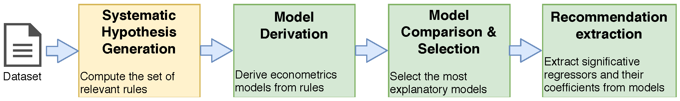
To validate the approach, we compare the recommendations returned by our methodology and those returned by rule mining alone against the ‘ground truth’ used to generate the synthetic datasets. More precisely, we compute the fraction of correct models returned by our methodology as the ratio of the number of models involving significant regressors that indicate (at least some) true discriminatory factors among the variables over the total number of models returned by the approach. To compare this outcome with the one obtained using rule mining, we compute the ratio of the number of rules indicating (at least some) true discriminatory factors over the total number of mined rules.

To this end, we first derive for each model the set of significant regressors along with their coefficients. Then, we compare each regressor with the set of variables describing the discriminated groups. This comparison can return five different outcomes: (a) Exact, indicating that the set of significant regressors of the model involve all and only the variables characterizing one of the discriminated groups; (b) Too general, indicating that the set of explanatory variables in the regressors is a strict subset of the set of variables characterizing one of the discriminated groups; (c) Too specific, indicating that the set of explanatory variables in a regressor is a strict superset of the set of variables characterizing one of the discriminated groups; (d) Partial, indicating that the set of explanatory variables in the regressor overlaps with the set of variables characterizing one of the discriminated groups (but it is not a superset); (e) Off target, indicating that there are no significant regressors involving any variable characterizing a discriminated group. The output of rule mining is classified in the same way, by comparing the set of variables reported in a rule against the set of variables describing the discriminated groups. For a fair comparison, we only considered the variables involved in the antecedent of the rules; indeed, we are interested in determining whether a group shows signs of discrimination, rather than specifying whether it is a positive or negative discrimination.

We only consider exact and too general recommendations to be useful recommendations, since they include the true discriminated group, and therefore provide the analyst with a first, non-misleading indication of possible discriminatory relations. In contrast, the other categories of output are undesirable since, even if some do return part of the actual discriminatory group, the whole discriminated group cannot be identified as it is not included in the recommendation. Therefore, we compute the fraction of useful recommendations as the number of Exact and Too general models (rules) over all returned models (rules).

In addition to comparing the returned models against the ground truth, we also compare rule mining and regression analysis in terms of the number of output rules and regressors, respectively. The goal is to assess the capability of our approach to reduce the outcome complexity, thus making the analysis more accessible for a human analyst.

4.1.3. Results

Models vs. rules.

Table 5. Min, max, mean, median, first and third quantile of the number of rules (first group of rows) and models (second group of rows) obtained in each experiment.

	Metric	Min	1st Q	Mean	Median	3rd Q	Max	sd
Rule mining	N_rules	0	0	12.87	4	13.25	139	23.74
	Exact	0	0	1.01	1	2	3	1.15
	Too general	0	0	1.77	0	3	7	2.38
	Too specific	0	0	3.52	0	2	64	9.99
	Partial	0	0	6.58	0	5	121	14.24
	Off target	0	0	0.00	0	0	0	0.00
Our approach	N_models_tot	0	0	4.98	4	8	16	4.72
	N_models_sel	0	0	1.05	1	2	6	1.11
	Exact	0	0	0.35	0	1	5	0.65
	Too general	0	0	0.53	0	1	6	1.03
	Too specific	0	0	0.18	0	0	2	0.39
	Partial	0	0	0.00	0	0	0	0.00
	Off target	0	0	0.00	0	0	0	0.00

reports descriptive statistics of the results over all experiment runs.

The first set of rows reports the statistics for association rule mining, whereas the second set reports the statistics for our approach. We first observe that the number of rules is significantly larger than both the number of total models (i.e., the models derived from the set of rules) and that of selected models (i.e., the models returned in output by our approach). Furthermore, the number of the selected models is, on average, four times smaller than the overall number of models. The average experimental run produces approximately 12.87 rules, with a maximum of 139. The relatively high standard deviation (with respect to the mean) indicates that the number of rules in output can vary by large amounts across experimental setups. In contrast, the number of total (selected) models per experimental setup is, on average, more than two (twelve) times smaller, similarly to what can be observed for the maximum. The low standard deviation indicates a relatively stable output across experiments, especially for the selected models. Overall, this indicates that the model selection procedure appears to be removing a large number of rules but says little about the correctness of this process.

A first indication of the correctness of this process can be derived by evaluating of the number of exact, too general, too specific, partial, and off target rules/models in output of our method. Considering the obtained rules, we observed that association rule mining never returns off target recommendations. Moreover, it is able to identify, on average, at least one correct recommendation, either in terms of exact or too general recommendations. However, comparing these numbers with the overall average number of rules returned, these recommendations are likely to be hidden in a multitude of misleading recommendations. In fact, the results show that rule mining tends to return a much higher number of undesirable recommendations; on average, we obtain 3.52 too specific and 6.58 partial recommendations.

On the other hand, we observe that our approach returns a higher number of max exact recommendations. This is because a regressor (matching the ground truth) can be significant in multiple models. In general, we observe a similar distribution in the first and second quartile, even though the mean and median values show in general a lower overall capability of our approach to identify relevant groups under most circumstances (the median of Exact is 0). However, this minimal loss in detection is compensated by a large reduction in false positives to investigate. Moving to higher quartiles, we observe that our approach never returns partial or off target results, and generates much less too specific and too general recommendations. Overall, the results suggest that our approach is able to generate a more accurate output. However, this clearly depends on the number of discriminated groups, and results may vary significantly depending on the noise and overlap introduced in the synthetic datasets.

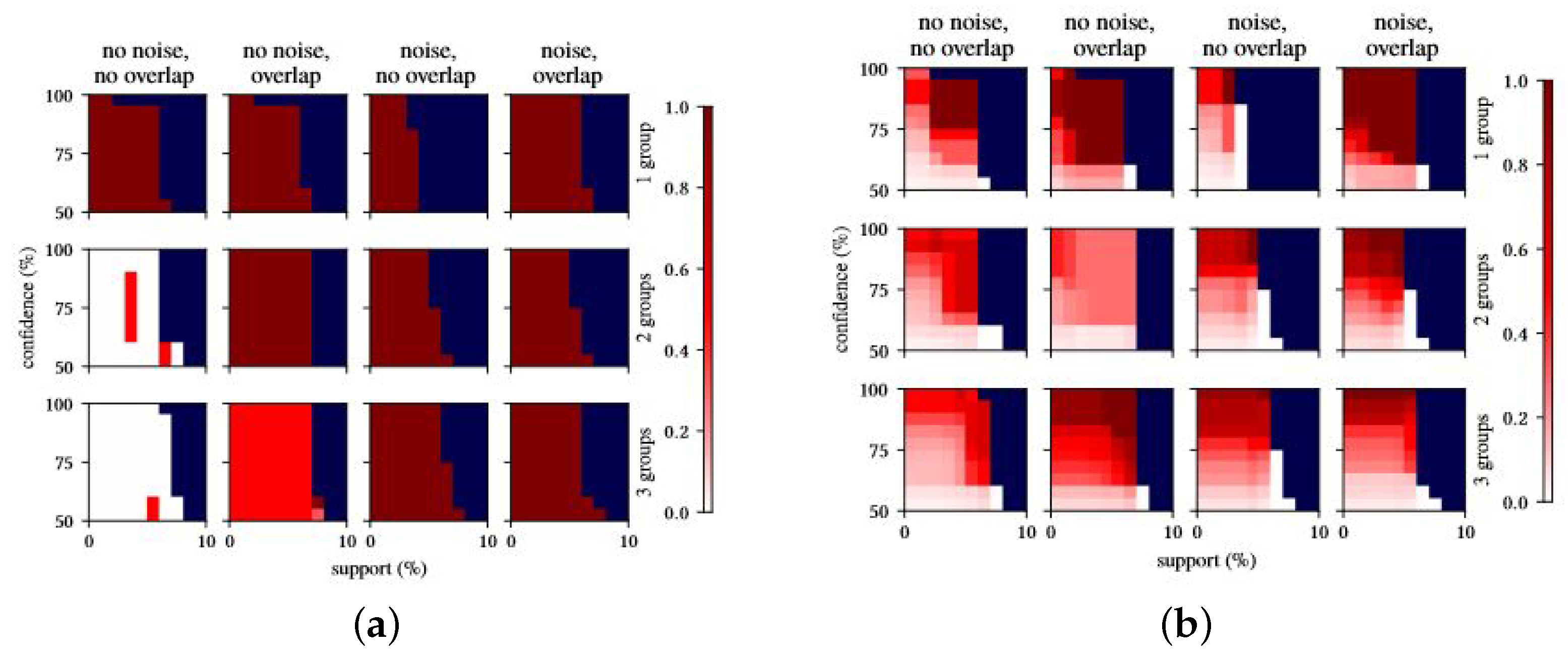
Figure 3 shows the density of ‘useful’ recommendations provided by rules mining and our approach, respectively, across our experimental conditions.

Results are arranged in a matrix, where each box represents a set of experiments with varying confidence and support levels (on the y and x axis, respectively, values are reported as percentages); the four columns correspond to the four combinations of noise and overlap, whereas the three rows correspond to the number of discriminated groups in the dataset. Recall that overlap does not impact the results when a single discriminated group is considered. The difference in the recommendations obtained for this dataset are mostly due to randomness in the data generation process. We reported them anyway for the sake of completeness. Within each box, each square corresponds to a combination of support and confidence thresholds. Squares are colored on the basis of the density of useful recommendations for the given combination of support and confidence. A darker color indicates a higher density (and vice versa). Blue cells represent support–confidence combinations from which no significant rules/regressors were obtained (resulting in a denominator of zero), and white cells represent support–confidence combinations for which no exact or too general recommendations were obtained.

We observe that, across almost all experimental setups, our approach produces a much higher density of relevant recommendations compared to rule mining alone. This confirms the observations made from Table 5; namely, rule mining tends to return a high number of recommendations, in which useful recommendations are hidden among the others. Our approach, instead, provides almost only useful recommendations in almost all performed experiments, with the exception of the experiments involving two and three discriminated groups with no noise and no overlap (first column of the second and third sets of experiments). While this might seem counter intuitive, delving into the corresponding dataset, we find that the over-imposed constraints for data generation turned out to produce unrealistic relations that significantly reduce the discriminating effects of the chosen variables. For more than one discriminated group, and in the absence of noise and overlap, the variable values used for the discriminated groups only occur for subjects fitting the related context. For example, in the experiments with two discriminated groups, we have discriminating context groups, “SpeakLanguage =Y” and “PreviousRole =Employee”. Because of the generation constraints, there are no subjects assuming both these values. This creates the rather unrealistic situation whereby the value of one variable precludes another variable to assume some values. Our approach (correctly) detects a strong correlation among context variables SpeakLanguage and PreviousRole. This leads to the generation of too specific recommendations for most of the support–confidence thresholds, with some exceptions mostly due to the randomness of data. We observe a similar though not as strong effect on the experiments with overlap and no noise. The constraint on the noise led to obtain some correlations between some context group values which in turn led to generate some misleading recommendations. Nevertheless, the overall density values remain high. We point out that the presence of such correlations is a by-product of the data generation constraints and is unlikely to represent a realistic situation under real-life conditions. Therefore, we do not expect this behavior to affect the reliability of the recommendations provided by the approach in real-life contexts.

It is worth noting that, while we observe performance to significantly vary for rule mining depending on the support/confidence thresholds, our approach proved to be more stable, keeping a constant level of density in almost all cases. This is in line with previous observations that rule mining is sensitive to parameterization, and that choosing the correct parameter configuration largely depends on unknown structures in the data. By contrast, our approach performs well across the board. This effectively removes the need for fine-tuning the support and confidence thresholds for rule selection, with regression model selection doing the larger part of the heavy lifting required to cherry-pick relevant rules and discarding imprecise ones.

Regressors vs. rules. The previous paragraph discussed the results obtained at the regression models level. Here we focus on the obtained regressors.

Table 6. Descriptive statistics for rules and regressors in the experiment runs with synthetic data.

Metric	Min	1st Q	Mean	Median	3rd Q	Max	sd
N_rules	0	0	12.87	4	13.25	139	23.74
N_regr	0	0	2.11	2	4	6	1.93

shows descriptive statistics about rules and regressors obtained for the tested datasets.

The table shows some interesting trends. First, we observe much more variation in the number of rules than in the number of regressors (sd = 23.74 and 1.93, respectively), and that extreme values far away from the median are more likely to appear in the former than in the latter distribution. This confirms that the outcome of our approach is much more stable than the rule mining outcome. Furthermore, it is straightforward to see that, on average, the number of regressors is significantly lower than the number of rules. This is particularly evident from the mean value, equal to 12.87 for the rules, while the mean number of regressors is 2.11, with a six-fold reduction. An even stronger reduction can be observed considering the maximum values (139 for the rules, 6 for the regressors).

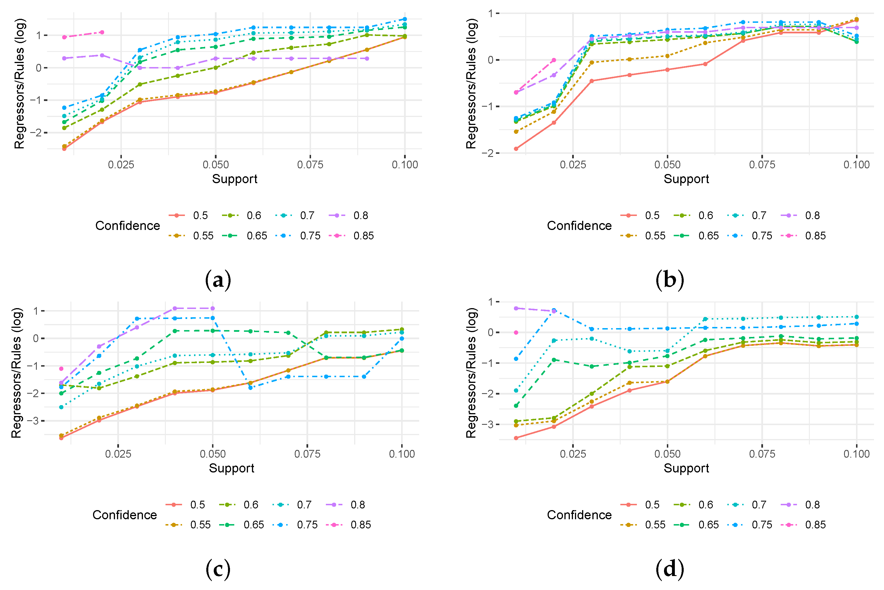
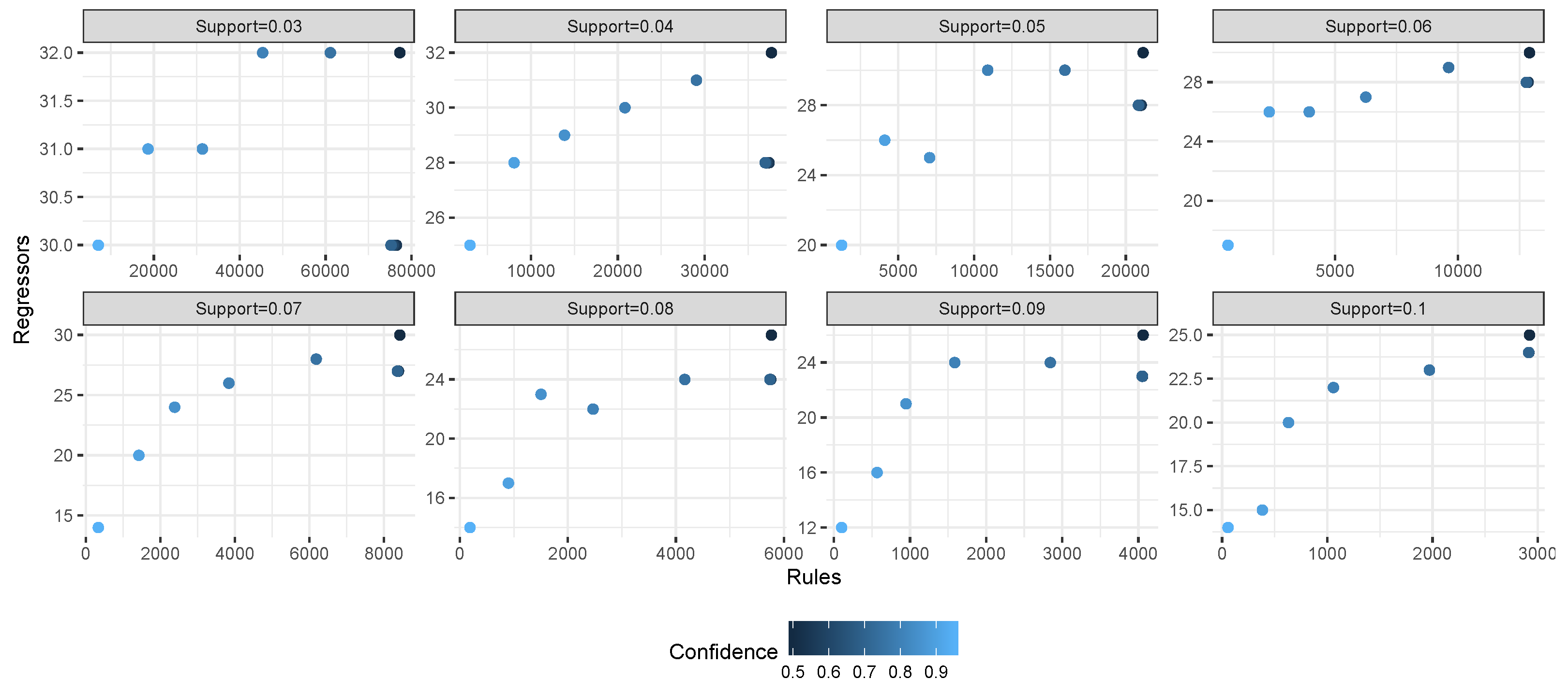
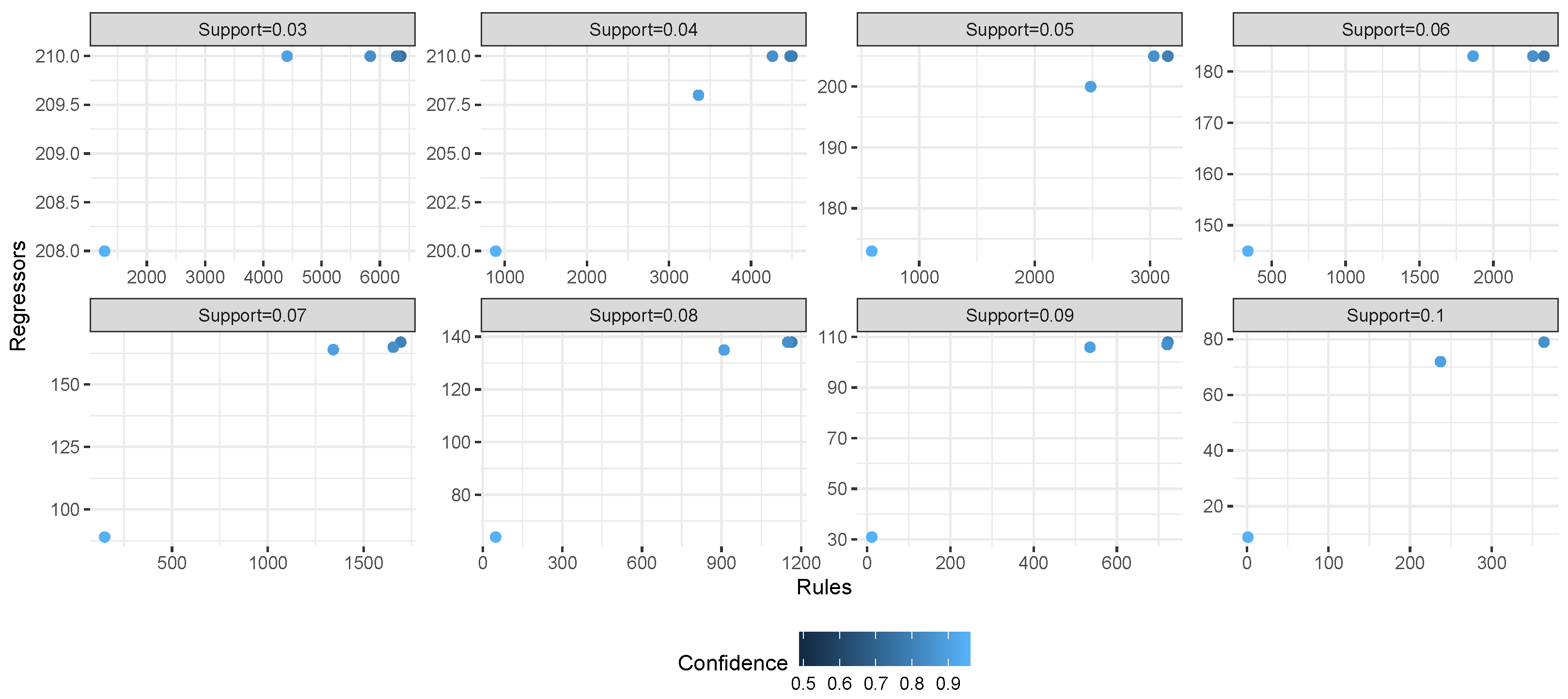
Figure 4 reports the relation between regressors and rules across the experiments for each dataset. Each grid corresponds to a single experimental setting (i.e., to one combination of support and confidence threshold); the x axis shows the number of extracted rules, while the y axis shows the number of extracted regressors. Different symbols and colors are used to represent the complexity of the dataset. A common trend for all datasets is that the number of rules exceeds the number of regressors for at least one order of magnitude at low support/confidence thresholds. Even when increasing the support/confidence thresholds, for most of the tested configurations, the number of rules was at least twice the number of regressors.

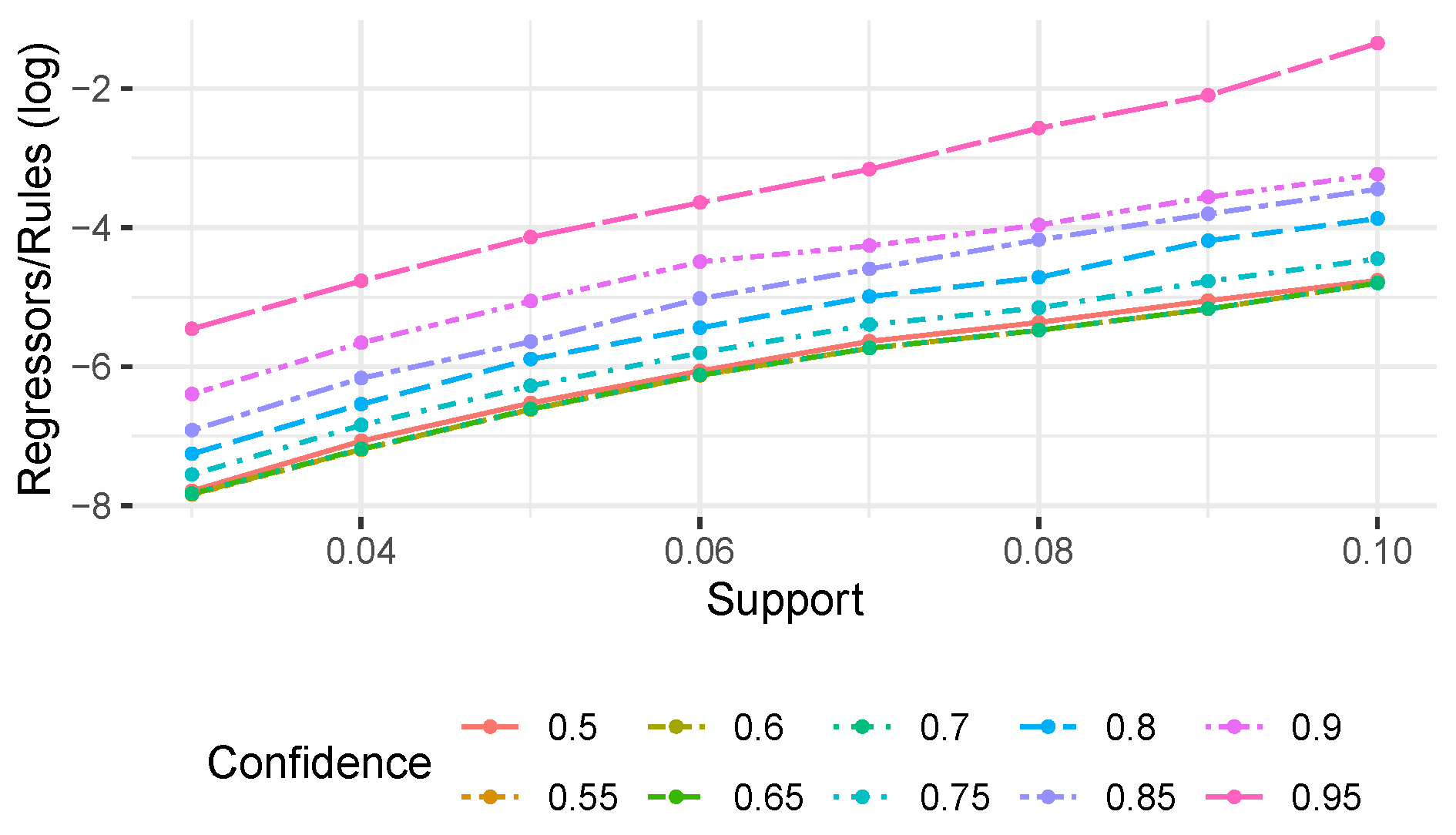
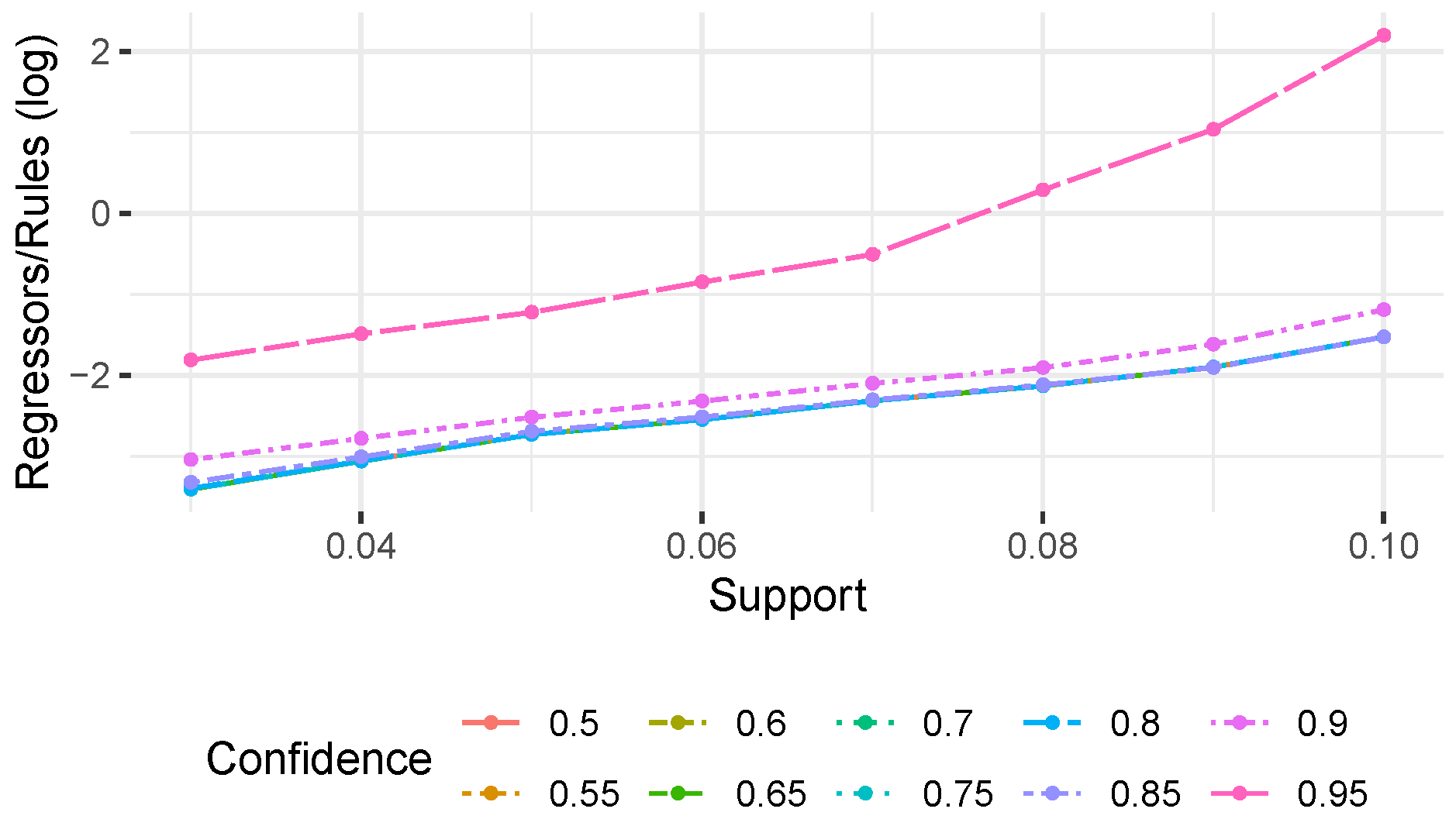
To visualize the order of magnitude in the difference between regressors and rules, Figure 5 reports (on a log scale) the ratio between regressors and rules for each experimental setting (without considering configurations where no rules were found). We observe that the datasets involving noise are also the ones in which we observe a stronger difference between the number of rules/regressors. In both datasets, we obtained at most the same numbers of regressors and rules, while in most of the configurations, the number of regressors is significantly lower (up to a three-fold reduction compared to the number of rules). For the datasets without noise, instead, while we still obtain overall less regressors than rules, this reduction is quite strong only for low support/confidence thresholds, and becomes less and less evident while increasing the thresholds. For the first dataset, the number of regressors exceeds, even though just slightly, the number of rules in few configurations. This is consistent with the characteristics of the used datasets; indeed, the datasets with no noise are also the ones more favorable to rule mining which, with high support/confidence thresholds, is able to return a limited number of rules. Nevertheless, overall these results show that the use of regression analysis reduces up to three times the number of generated bias candidates.

Summarizing, the results show that our approach is able to significantly reduce the number of recommendations provided by rule mining without losing knowledge on the potential bias in the data. The approach also returned consistent results across varying support and confidence thresholds, thus showing to be robust with respect to parametrization. Interestingly, the cases where the approach showed more difficulties are the ones where the data generation procedure created very strong and undesired correlations among variables between which no correlation was intended. We discuss the limitations of the proposed method, such as spurious correlations, in Section 5.

4.2. Approach Application to Two Real-Life Use Cases

In this section, we discuss the results obtained by applying our approach to two real-life datasets which were used in previous work on discrimination detection: the German credit dataset [15], used, e.g., in [4,16,17], and the Crime and Communities dataset [18], used, e.g., in [16,19]. In the following, we present results related to configurations in which support varies between 3% and 10% with a step of 1% and confidence varies between 50% and 95% with a step of 5%. Exploring very low support values turned out to be not feasible with the current implementation of our approach, in terms of hardware and time constraints. Therefore, we did not test our approach for values of support equal to 1% and 2%. We argue that this choice does not significantly impact the validity of the performed results, since it is not unreasonable to discard very infrequent associations when addressing real-life cases. In addition, the validation of our approach on synthetic datasets has shown that it is robust with respect to the parameterization of support.

4.2.1. Use Case on Credit Risk

Dataset and Settings. The German dataset consists of 1000 records representing the assessment of credit risk (good or bad) of bank account holders [15]. The dataset encompasses 21 variables, grouped according to the following categories: personal properties (checking account status, duration, savings status, property magnitude, type of housing), properties related to past/current credits and requested credit (credit history, credit request purpose, credit request amount, installment commitment, existing credits, other parties, other payment plan), properties related to the employment status (job type, employment since, number of dependents, own telephone), and personal attributes (personal status and gender, age, resident since, foreign worker). We discretized the numeric attributes as suggested in [4]. Following [17], we considered the decisional process to be affected by discrimination if the final decision was influenced by the fact that the holder belongs to one or more of the following subgroups: non-single female, older than 52 years and foreign worker.

Results.

Table 7. Descriptive statistics of the experiment runs for the credit dataset.

Metric	Min	1st Q	Mean	Med.	3rd Q	Max	sd
#rul	54.0	2894.0	14,668.1	5971.5	19,166.5	77,219.0	20,004.6
#mod	12.0	117.25	373.1	231.5	491.25	1560.0	386.3
#regr	12.0	23.8	25.3	26.5	28.2	32	4.7

reports the descriptive statistics for the 80 experiment runs for varying levels of support ($[0.03,0.10]$ with steps of $0.01$) and confidence ($[0.5,0.95]$ with steps of $0.5$). We observe that the number of rules in the output is higher but resembles the same distribution as the number of derived regression models. Absolute values are, as one would expect, much higher for real datasets than for the experiment with synthetic data. The median experimental setting produces 5971.5 rules and 231.5 models. The stable ratio of models to rules between the two settings (synthetic and real) suggests that the pre-conditions for the two experiments are comparable. If we focus on the significant, unique regressors, we observe a stronger reduction; indeed, thanks to model selection, we obtain a median and a maximum of 26.5 and 32 regressors to consider (as opposed to, respectively, 5971.5 and 77,219 rules).

Figure 6 reports the relation between regressors and rules across experiments. We can observe that while the results obtained using rule mining vary significantly for different support and confidence settings, regressors turn out to be quite stable, with variations of the order of a few dozens across all experiments. Furthermore, the number of rules exceeds the numbers of regressors of a factor ranges from 10 to 1000, depending on the support level.

Figure 7 reports the (log) ratio between models and rules for each experimental setting. At every level of support and confidence, the number of regressors is, on average, notably smaller than the number of rules. The stability of the results given by our approach is consistent with what we observed in Section 4.1. Nevertheless, the reduction is especially strong at a low level of confidence and support. These results point out that the number of regressors remains manageable for being analyzed by a human policy maker, whereas the number of rules explodes. This suggests that our approach can be very effective in practice to obtain usable and statistically significant indications of biases in the data without the need to fine-tune the support/confidence levels in input to rule mining. The overhead in terms of output from low support and confidence levels is limited, whereas one is not incurred in the risk of removing potentially relevant rules.

The results discussed to date show the capability of the approach to significantly reduce the space of candidate hypotheses, with respect to classic association rule mining. Exploring these hypotheses to detect the presence of actual biased relations is, at this point, up to the human policy makers. A detailed analysis of the detected regressors would not be possible here, for the sake of space. Nevertheless, in the following, we briefly discuss how regressor coefficients, together with their confidence intervals, can be used to further aid the policy maker in her analysis.

To this end, let us consider the configuration with support equal to 0.09 and confidence equal to 0.9. Figure 8 shows the confidence intervals of the corresponding regressors related to the three variables under investigation in our experiments, i.e., Age, Personal status and Foreign worker. The y axis shows the coefficient values; the blue cross represents the estimated value of the coefficient of one regressor and the blue line corresponds to its 95% confidence interval. The light-blue without crosses lines group regressors belonging to the same models. The number of lines per model depends on the domain of the corresponding variable. Both Age and Personal status have four different values; therefore, here we have three lines for every model corresponding to the values not used for the baseline in the regression. Foreign worker, instead, is a binary value; hence, each single line belongs to a different model.

First, we observe that the three variables occur in the result set with different frequencies: we found 10 models containing Age, 79 containing Personal status and 528 containing Foreign worker. By observing the trend of confidence intervals for each variable, one can already spot which candidate hypotheses look more interesting and which ones, instead, could likely be discarded. For instance, all confidence intervals for Age span across both negative and positive values, indicating no clear effect of Age on the outcome variable. This indicates that Age is not a discriminatory factor on its own. It is worth noting that the variable Age occurs in several rules. Therefore, by applying rule mining alone, one might deem this variable to be influential for the decision, although it has actually no statistically significant impact on the output.

The situation is different for the other two variables. For the sake of clarity, Figure 9 zooms in on some models for both the variables.

For Personal status, we focus on the first three models since we observe a stable trend from the overall figure, which suggests that similar insights can be derived from any group of models. For Foreign worker, instead, while we still observe a similar trend across the models, there seems to be more variability for the first few models; therefore, we decided to focus on the first ten. Figure 9a shows the third line of every model, corresponding to the value male_single which is always above 0. This suggests that this value of Personal status has a significant and positive impact on the decision, even though not a very strong one. This suggests that male, single candidates are significantly more likely to receive a positive risk class than the baseline group, i.e., non-single females. Similarly, for Foreign worker, we can see that the confidence interval is always below 0; namely, this regressor shows a significant and negative impact of being a foreign worker on the decision, with respect to the baseline group of non-foreign workers. Such an impact is relatively strong: in many cases, the likelihood of a positive decision was reduced up to 80%. These observations suggest that both these variables should be further investigated.

Figure 8 also shows that the regressors exhibit the same trend for every model in the result set. This suggests that the behavior of these variables may somehow be considered as a global behavior or, at least, as a behavior valid for all identified groups of features. Further investigation may still be conducted to explain visible differences in terms of the coefficient values, for example, in the first set of models involving Foreign worker. We argue that such a representation would also provide the analyst with a valid means to detect groups in which regressors behave differently. In contrast, none of these considerations could have been drawn using rule mining alone. Using rule mining, the analyst can only derive the itemsets that are frequently related to a given value of the outcome variable, but no support was provided to analyze their statistical impact.

4.2.2. Use Case on Crime in Communities

Dataset and Settings. The Crime and Communities dataset contains 1994 records of communities described by socio-economic and demographic factors, including their crime rates [18]. In particular, the dataset involves 128 numerical variables, related to, e.g., average income, average household size, percentages of different ethnic groups, percentages of people at different degree of education and percentage of people using public transport. We preprocessed the dataset by performing common data cleaning tasks; namely, we removed variables involving missing values, as well as variables involving a single value, since they would have only led to noise in the analysis. The cleaned dataset involved 91 attributes. We applied supervised discretization to convert numerical variables into categorical; more precisely, we used the default settings of the supervised discretization technique implemented in Weka (https://www.cs.waikato.ac.nz/ml/weka/, Last access 16 March 2022), which strives to determine the most discriminative intervals with respect to the class.

As in [19], we selected variable ViolentCrimePerPop as the class attribute, where values lower than 20 represent the positive decision and values equal to or greater than 20 represent the negative decision. Among the four values of the variable racePctBlack, the sensitive item is: $\mathtt{racePctBlack}=[0.375,1]$. Accordingly, the decisional process is considered to be affected by discrimination if the fact that black people are the majority in the community has influenced the final decision.

Results.

Table 8. Descriptive statistics of the experiment runs for the Crime and Communities dataset.

Metric	Min	1st Q	Mean	Median	3rd Q	Max	sd
#rul	1.0	722.0	2245.0	1693.0	3153.0	6355.0	1879.7
#regr	9.0	108.0	157.4	167.0	205.0	210	52.1
#mod	1.0	658.0	1721.3	1565.0	2696.0	3570.0	1170.3

reports the descriptive statistics for the 80 experiment runs for varying levels of support ($[0.03,0.10]$ with steps of $0.01$) and confidence ($[0.5,0.95]$ with steps of $0.5$). The number of models, while being consistently lower than the number of rules, is significantly higher those we obtained in the German dataset, approximately in the same order of magnitude as the number of rules. The number of regressors, on the other hand, shows a reduction in more than ten times with respect to the number of rules (models), along with a smaller standard deviation (and, therefore, a more stable output). The median obtained for rules and models in this experiment setting produces 1693 and 1565, respectively, while the median value for the regressors is 167. Moreover, we observe a maximum of 210 regressors to consider (as opposed to, respectively, 6355 rules and 3593 models).

Figure 10 reports the relation between regressors and rules across experiments. We observe a trend similar to the one we observed for the German dataset, i.e., a strong variability in the rule mining results for different support and confidence settings, despite relatively stable regressor outputs. Furthermore, in this case, the number of rules exceeds the number of regressors of a factor ranging from 10 to 1000, depending on the support level. A notable exception, however, can be seen in the experiments with support higher than 0.8 and maximum confidence. This is due to the fact that, in these cases, only a few rules were mined, with the result that the output of rule mining is in this case comparable with that obtained using our approach. In one case, for the configuration with the highest threshold, only one rule was mined, from which nine significant regressors were extracted.

Figure 11 reports the (log) ratio between regressors and rules for each experiment setting. These results are consistent with what we observed for both the synthetic and German datasets: especially for low levels of these settings, there is a strong reduction in the candidates in the result set. Across all support levels, high confidence levels generate a higher number of regressors (with respect to generated rules) than at low confidence levels. At a high confidence level, the number of regressors exceeds that of rules by a factor of 2–3 for support levels higher or equal to 0.8, and reduces well below zero at lower confidence levels. This is in line with the observation made for Figure 10 where we pointed out that in some settings, a few rules were obtained, which generated a comparable or higher number of regressors.

Figure 12 shows the confidence intervals for the regressors obtained for a support equal to 0.09 and confidence equal to 0.9. Among the 535 models containing the variable racePctBlack, the figure only reports the first 50 models for the sake of readability. These models show common trends among all models, but they also show some notable outliers. First, regressors in the first 42 models show a significant positive impact on the decision variable. Delving into greater detail, we observe that the third line of each model which corresponds to the highest percentage of black people in the community is the one with the largest impact on the class. Therefore, overall these models seem to suggest that if the percentage of black people increases, the possibility of being classified as a dangerous area also increases. However, the magnitude of the impact does seem to change in some models, moving from a strong impact (more than three-fold) to a marginal and even negative impact. For example, a model in Figure 12 shows that the first two values are close to zero; and the third line actually goes below 0, thus pointing out that this value is not significant at all for this model. It is worth noting that in the remaining set of models we analyzed (not reported here for the sake of space), the racePctBlack regressor always has a strong impact with the same dynamics we described above. Starting from these observations, the policy maker can actually recover the corresponding model to investigate the reasons underlying the observed differences.

5. Discussion

In this section, we elaborate upon some key observations obtained from our experiments and discuss the limitations of our approach.

Effective candidates generation. The results show how the combination of rules mining and regression analysis allow one to overcome the disadvantages of each method applied individually. First, we stress that, without the rule mining contribution to the methodology, the model testing using regression analysis would have failed to identify interesting relations. To double-check this, during the first stages of this work, we attempted to generate ‘optimal’ models through backward and forward model generation (ref. Section 2.2), leading to uninterpretable results, and oftentimes failing to target ‘sensible’ variables of interest. The systematic hypothesis generation process effectively implemented using rule mining allows focusing on models describing the phenomenon of interest (e.g., potential discrimination in a group or population). At the same time, the rigorous statistical evaluation employed for model selection allows our method to discard a large amount of ‘false positives’ returned by rule mining whose output, indeed, turned out to be very noisy (cf. Figure 3). Overall, we observe some improvements when increasing the support and confidence thresholds. However, being constrained to the use of high values of support and confidence is in general not desirable, since it can lead to some interesting dependencies being missed, especially when investigating possible discrimination cases. These limitations appear to be overcome or significantly reduced with the use of regression models for model derivation and selection. This approach scored relatively well in all experiment settings. Even though there are few configurations in which the approach could not detect any interesting bias, this was due to perfect correlations among unrelated variables, obtained by the data generation procedure and not so likely to occur in real scenarios.

Robustness with respect to parameter tuning. Another notable positive aspect of the approach is that performances are much less dependent on parameterization. In this respect, the forest structure used for model comparison requires pairwise comparisons between models, which rapidly increases as more models are generated by the rules. Nevertheless, our approach proved to be able to detect biased relations even with low values of confidence and support; this suggests that it is suitable also to explore bias-affecting minorities. Different data structures and heuristics for model comparison (e.g., eliminating models with irrelevant variables from different branches) could be employed to decrease the computational overhead. Nonetheless, the advantage of limiting the impact of blind fine-tuning from the procedural setup provides the desirable advantage of assuring that precise (as defined above) results can be expected as long as support is small. This gives the analyst some leeway on the concern about setting the thresholds for support and confidence.

Understandability of the extracted recommendation. Our experiments show that the number of regressors remains manageable for being analyzed by a human policy maker, whereas the number of rules explodes. This suggests that our approach can be very effective in practice to obtain usable and statistically significant indications of bias. We also show how plotting the obtained regression models represents a useful aid to the policy maker to grasp additional information on which variables/models can be shown to the class to have interesting correlations. In particular, we discussed how confidence intervals can be exploited to obtain an informative overview on relations existing within models of a single configuration, providing the base for further exploration.

Assumptions and limitations. The proposed approach can only detect the statistical evidence of bias in cases where the data generation process is sufficiently biased to generate that evidence. This is unavoidable in any empirical approach. In cases where little data exist for the investigation, the statistical detection of small bias effects may fail, as evidence may be attributed to chance alone. In those cases, other approaches such as qualitative methods may be more appropriate. Similarly, while our approach proved to be less sensible to parameter tuning than rule mining, the impact of tuning can still be relevant when addressing datasets with severely underrepresented groups. In the absence of a ground-truth on discrimination levels and groups, our approach to generate a synthetic dataset aims to striking a balance between extreme cases, and considering general guidelines for discriminative actions (e.g., the four-fifths rule [20]) as guiding principles. Whereas a more thorough sensitive analysis for tuning parameters may provide additional estimates of method performance in more extreme cases, those estimates are likely to be misleading because of unknown confounding factors affecting the data. To showcase the applicability of our method, we therefore decided to not make any strong assumptions about the nature of our synthetic dataset.

Another important observation concerns the presence of so-called “proxy” rules and “redundant” rules. The first ones are rules which, while not directly classifiable as biased decisions, actually lead to biased and unfair decisions [4,21]. Redundant rules, instead, are rules that cover the same (or a similar) set of samples of one or more other rules in the dataset. The presence of these rules is typically due to the presence of some correlations within the features and can lead to misleading and/or unreliable outcomes. In our experiments, we assume that all the features relevant for the decisions are present in the dataset, and there is no strong spurious correlation among the features set. We plan to investigate these aspects in future work. Nevertheless, we would like to point out that some mitigation strategies can be applied. For example, proxy rules could be detected by interviewing, when possible, domain experts to understand the relevance and possible hidden use of the features of the dataset. On the other hand, to prevent the generation of redundant rules, one can apply, for example, feature selection approaches, or pruning the redundant rules using approaches such as [22].

6. Related Work

This section provides an overview of the research related to model transparency, in particular features selection, association rule mining, and discusses approaches based on combining association rule mining and regression analysis. A summary of these approaches with respect to the desiderata in Section 2 is given in

Table 9. Comparison of the related work with respect to the desiderata for bias detection presented in Section 2, where ● means “support”, ◐ “partially support”, ○ “no support”. The asterisk (‘*’) indicates that the requirement is only supported by some approaches.

	Data Agnostic	No Param. Tuning	Feature Level	Feature Value Level	Change Impact
Association Rule Mining	●	○	○	●	○
Features selection
Filter Methods	●	○	●	○ *	○
Wrapping Methods	◐	○	●	○	○
Embedded Methods	◐	○	◐	○	○
Combined approaches	◐	○	●	◐	●
Our work	●	◐	●	●	●

.

The increasing adoption of classifiers to support human decision-making processes has led to an increasing importance of the transparency of the models generated by machine learning techniques. A recent survey on this topic [23] identifies two categories of problems related to model interpretability, i.e., a black-box explanation problem, where decisions returned by a black-box classifier are analyzed to construct an explanation, and a transparent box design problem, where the goal is to develop interpretable, white-box classifiers. Our work is related to approaches in the first category, which can be further refined in three subgroups: model explanation aims to provide human-interpretable models capable of mimicking the behavior of the original classifiers [24,25,26]; outcome explanation aims to build local models explaining predictions made on single instances [27,28]; model inspection aims to provide a human understandable representation of some specific properties of the model and/or its predictions [29,30].

Our work is mainly related to model explanation, particularly so-called agnostic approaches (i.e., approaches that are not tailored to a specific classifier), which usually provide explanations in terms of features ranking. This problem overlaps with the feature selection problem, whose goal is to identify and remove those features that either do not have an impact on the classification or are “redundant”, i.e., they are correlated to other features [31,32,33,34]. These methods can be grouped into three main categories. Filter methods evaluate the discriminative power of features exploiting exclusively intrinsic proprieties (e.g., the statistical properties) of the data [35,36]. The outcome of a filter method can consist of either the set of features showing a correlation with the class above a user-defined threshold (so-called “univariate” methods), or groups of features showing the best trade-off in terms of correlations with the class and minimum correlations among each other (named “multi-variate” methods) [31,37,38]. Another class of feature selection methods consists of wrapping methods. Given a classifier, they look for the subset of features that provide the best results in terms of a classification quality metric, e.g., accuracy [39,40]. The search is performed either by adding or removing one feature at each iteration, then evaluating the obtained improvements. Wrapper methods usually perform significantly better than filter approaches; however, they are computationally intensive and thus, unsuitable for real-world applications characterized by a large feature space. Finally, embedded methods are feature selection approaches embedded in the classification process itself; namely, these approaches exploit an intrinsic model building metric to assess the importance of features during the construction of decision trees [41].

All three classes of feature selection techniques do not completely meet the desiderata identified in Section 2. Change impact analysis is only addressed by some embedding and filtering approaches, e.g., [42], while wrapping approaches mainly rely on classification accuracy. Only multi-variate filter approaches are data-agnostic. Wrapping and embedding methods only partially meet this desideratum: to obtain the best results, one should know the classifier used for the decisions being analyzed. All feature selection methods require parameter tuning. Analysis at the feature level is fully supported only by wrapping methods. Indeed, many filter and embedded methods only return the correlation values for a single feature; only few methods in these groups allow one to assess correlations between the class and groups of features. It is worth noting that none of the methods support the analysis at the feature value level.

A recent model transparency approach alternative to feature selection is presented in [43]. This approach aims to provide explanations related to some subspace of interest, i.e., groups of samples of the population presenting some characteristics of interest, usually represented in terms of itemsets. A set of classification rules is then derived for samples in those groups by means of a multi-objective optimization function taking into account factors such as rules overlapping, fidelity to the original classifiers behaviors, precision, etc. This work, however, has the same advantages and disadvantages of association rule mining (see Section 2.3).

Association rule mining has been largely applied to analyze decisional processes, especially for discrimination discovery [4,22]. Several metrics tailored to measure the impact of sensitive itemsets on the class have been proposed. In a seminal work on discrimination discovery [4], Ruggeri and colleagues introduced the notion of extended lift. This metric measures how the rule confidence varies with/without the discriminatory itemset, thus providing an evaluation of the relevance of this itemset. This approach, however, does not support any statistical validation of the discovered associations. To address this issue, several approaches have been proposed. Some focus on mining non-redundant rules by comparing each rule with its generalizations and discarding those rules, not showing any improvement in terms of support [44] or confidence [8]. Other approaches, instead, fall within the field of statistical association rule mining, i.e., they focus on mining statistically significant positive associations, ensuring that these associations are unlikely to be due to chance. Some approaches apply statistical tests to rule assessment metrics, e.g., the confidence intervals [45]. Statistical tests have also been used to validate feature-class correlations, filtering rules involving features with an insufficient/not significant level of correlations [9], or assessing possible correlations between itemsets and the class by means of hypothesis testing (e.g., [46,47,48]).

While these approaches do improve the statistical robustness of the discovered set of rules, they come with some drawbacks. Approaches exploiting relevance metrics only indirectly assess the statistical significance of the impact of the feature values on the class values. Moreover, the use of different metrics can lead to different results, and some commonly-used metrics also come with some drawbacks. For example, it is well known that rules whose consequent has a high support tend to have a high value of confidence, without this implying a real dependency among the antecedent and the consequent [46]. Furthermore, confidence allows measuring only one direction of the impact of feature values, i.e., positive correlations. In addition, all these approaches are mainly intended as filtering mechanisms. Overall, the support provided to the statistical validation of discovered association rules is still limited and not as mature as in other techniques, such as regression analysis. Indeed, the scope of the performed evaluation is only limited to the values of the explanatory variables that occur in the rule under analysis. Little or no support is provided to explore how the impact changes with respect to the different values of the variables.

The combination of associations rules and regression analysis is mostly unexplored; to date, only a few approaches have investigated potential advantages and applications. For instance, Changpetch and Lin [49] investigated the use of association rule mining to detect the set of the most interesting interactions to take into account when building a regression model. However, rule mining is only used to identify interactions among features. Moreover, only a single model is returned, which does not allow differentiating among different possible contexts in which discrimination could have occurred. It is also worth noting that a very aggressive rule filtering mechanism is adopted, so that only correlations with a strong support are considered, which is not always desirable when dealing with biases that involve small portions of the overall population. Other approaches exploit rule mining in the iterative building of the (best) regression model. For example, Jaroszewicz [50] defines so-called polynomial association rules to determine non-linear correlations among a set of (continuous) features and the class, and use an iterative regression model-building procedure that picks the best polynomial rule at each step to determine the factor to include in the regression model. Furthermore, in this case, the output consists of a single, ‘optimal’ model; moreover, polynomial rules are targeted to numerical domains. Other approaches combine their predictive capabilities in a single hybrid system to enhance classification performance. For example, Kamei et al. [51] showed an application to determine faulty modules, where samples described by a (set of) rules are classified accordingly, while samples for which no rules are available are classified according to a regression model. In this respect, the two classification models are built independently from each other. Combined approaches behave similarly to regression analysis, supporting statistical validation and analysis at both feature and feature values level. However, they require parameter tuning for the application of rule mining. They also bring some improvements in terms of data-agnostic requirement, since the use of rule mining enhances classic model selection techniques. However, as their goal is to detect the “best” model, it does not support the generation of multiple hypotheses, so that they cannot identify multiple contexts involving biases.

7. Conclusions

In this work, we proposed a methodology that leverages both association rule mining and regression analysis to uncover systematic biases in decisional processes. Specifically, our methodology uses association rule mining to systematically generate hypotheses of bias sources from an exploration of data. These hypotheses are then used to build regression models that provide statistically significant evidence about the impact of variables on the process outcome. The experiments show that our methodology overcomes the limitations of standard association rule mining and regression analysis. However, while being able to detect the population that is discriminated against, it tends to provide only an indication of the targeted set of observations, as opposed to giving a precise picture of targeted sub-groups. This is to be expected from any statistical analysis, as noisy data and sample sizes affect clearly have an impact on the prediction. Nonetheless, the ability of filtering out a large number of overly specific rules and focusing only on a few that are highly likely to cover the population of interest (or otherwise point towards it), enables policy makers and analysts to focus on groups of observations where future investigations and data collection are likely to uncover the specific effect. Furthermore, we showed how confidence intervals can be effectively exploited to grasp an overview of the most important detected relations, thus providing valuable guidance for the human analyst. In future work, we plan to address some of the limitations discussed in Section 5. In particular, we plan to investigate the combination of different rules’ redundancy reduction techniques with our approach in order to improve its robustness with respect to undesired correlations among features. In addition, we plan to apply our method in other contexts, for example to uncover indicative patterns of compromise in network traffic based on a security event generated by network security sensors as recorded by a security operation center.

References

1. Sundaramurthy, S.C.; McHugh, J.; Ou, X.; Wesch, M.; Bardas, A.G.; Rajagopalan, S.R. Turning contradictions into innovations or: How we learned to stop whining and improve security operations. In Symposium on Usable Privacy and Security; USENIX Association: Berkeley, CA, USA, 2016; pp. 237–251. [Google Scholar]
2. Sundaramurthy, S.C.; Bardas, A.G.; Case, J.; Ou, X.; Wesch, M.; McHugh, J.; Rajagopalan, S.R. A human capital model for mitigating security analyst burnout. In Symposium On Usable Privacy and Security; USENIX Association: Berkeley, CA, USA, 2015; pp. 347–359. [Google Scholar]
3. Chen, T.R.; Shore, D.B.; Zaccaro, S.J.; Dalal, R.S.; Tetrick, L.E.; Gorab, A.K. An organizational psychology perspective to examining computer security incident response teams. IEEE Secur. Priv. 2014, 12, 61–67. [Google Scholar] [CrossRef]
4. Ruggieri, S.; Pedreschi, D.; Turini, F. Data mining for discrimination discovery. ACM Trans. Knowl. Discov. Data 2010, 4, 9:1–9:40. [Google Scholar] [CrossRef] [Green Version]
5. Tversky, A.; Kahneman, D. Judgment under Uncertainty: Heuristics and Biases. Science 1974, 185, 1124–1131. [Google Scholar] [CrossRef]
6. Agrawal, R.; Imieliński, T.; Swami, A. Mining Association Rules Between Sets of Items in Large Databases. SIGMOD Rec. 1993, 22, 207–216. [Google Scholar] [CrossRef]
7. Field, A. Discovering Statistics Using IBM SPSS Statistics; Sage: Thousand Oaksm, MA, USA, 2013. [Google Scholar]
8. Bayardo, R.J.; Agrawal, R.; Gunopulos, D. Constraint-based rule mining in large, dense databases. Data Min. Knowl. Discov. 2000, 4, 217–240. [Google Scholar] [CrossRef]
9. Shaharanee, I.N.M.; Hadzic, F.; Dillon, T.S. Interestingness measures for association rules based on statistical validity. Knowl.-Based Syst. 2011, 24, 386–392. [Google Scholar] [CrossRef]
10. Genga, L.; Allodi, L.; Zannone, N. Unveiling systematic biases in decisional processes: An application to discrimination discovery. In Proceedings of the Asia Conference on Computer and Communications Security, Auckland, New Zeland, 7–12 July 2019; ACM: New York, NY, USA, 2019; pp. 67–72. [Google Scholar]
11. Liu, B.; Hsu, W.; Ma, Y. Integrating classification and association rule mining. In Proceedings of the International Conference on Knowledge Discovery and Data Mining, New York, NY, USA, 27–31 August 1998; AAAI Press: Palo Alto, CA, USA, 1998; pp. 80–86. [Google Scholar]
12. Tan, P.N.; Kumar, V.; Srivastava, J. Selecting the right objective measure for association analysis. Inf. Syst. 2004, 29, 293–313. [Google Scholar] [CrossRef]
13. Webb, G.I. Discovering significant rules. In Proceedings of the SIGKDD International Conference on Knowledge Discovery and Data Mining, Philadelphia, PA USA, 20–23 August 2006; ACM: New York, NY, USA, 2006; pp. 434–443. [Google Scholar]
14. Agresti, A. Categorical Data Analysis; John Wiley & Sons: Hoboken, NJ, USA, 2003; Volume 482. [Google Scholar]
15. UCI. Statlog (German Credit Data) Data Set. Available online: http://archive.ics.uci.edu/ml/datasets/statlog+(german+credit+data) (accessed on 20 December 2021).
16. Nasiriani, N.; Squicciarini, A.C.; Saldanha, Z.; Goel, S.; Zannone, N. Hierarchical Clustering for Discrimination Discovery: A Top-Down Approach. In Proceedings of the International Conference on Artificial Intelligence and Knowledge Engineering, Sardinia, Italy, 3–5 June 2019; IEEE: Piscataway, NJ, USA, 2019; pp. 187–194. [Google Scholar]
17. Pedreschi, D.; Ruggieri, S.; Turini, F. Integrating induction and deduction for finding evidence of discrimination. In Proceedings of the International Conference on Artificial Intelligence and Law, Barcelona, Spain, 8–12 June 2009; ACM: New York, NY, USA, 2009; pp. 157–166. [Google Scholar]
18. UCI. Communities and Crime Data Set. Available online: https://archive.ics.uci.edu/ml/datasets/Communities+and+Crime (accessed on 20 December 2021).
19. Qureshi, B.; Kamiran, F.; Karim, A.; Ruggieri, S. Causal discrimination discovery through propensity score analysis. arXiv 2016, arXiv:1608.03735. [Google Scholar]
20. Bobko, P.; Roth, P.L. The four-fifths rule for assessing adverse impact: An arithmetic, intuitive, and logical analysis of the rule and implications for future research and practice. In Research in Personnel and Human Resources Management; Emerald Group Publishing Limited: Bingley, UK, 2004. [Google Scholar]
21. Hajian, S.; Domingo-Ferrer, J. A Methodology for Direct and Indirect Discrimination Prevention in Data Mining. IEEE Trans. Knowl. Data Eng. 2013, 25, 1445–1459. [Google Scholar] [CrossRef]
22. Genga, L.; Zannone, N.; Squicciarini, A. Discovering reliable evidence of data misuse by exploiting rule redundancy. Comput. Secur. 2019, 87, 101577. [Google Scholar] [CrossRef]
23. Guidotti, R.; Monreale, A.; Ruggieri, S.; Turini, F.; Giannotti, F.; Pedreschi, D. A survey of methods for explaining black box models. ACM Comput. Surv. 2018, 51, 93. [Google Scholar] [CrossRef] [Green Version]
24. Augasta, M.G.; Kathirvalavakumar, T. Reverse engineering the neural networks for rule extraction in classification problems. Neural Process. Lett. 2012, 35, 131–150. [Google Scholar] [CrossRef]
25. Craven, M.; Shavlik, J.W. Extracting tree-structured representations of trained networks. In Advances in Neural Information Processing Systems; MIT Press: Cambridge, MA, USA, 1996; pp. 24–30. [Google Scholar]
26. Schetinin, V.; Fieldsend, J.E.; Partridge, D.; Coats, T.J.; Krzanowski, W.J.; Everson, R.M.; Bailey, T.C.; Hernandez, A. Confident interpretation of Bayesian decision tree ensembles for clinical applications. IEEE Trans. Inf. Technol. Biomed. 2007, 11, 312–319. [Google Scholar] [CrossRef] [PubMed]
27. Ribeiro, M.T.; Singh, S.; Guestrin, C. Why should i trust you: Explaining the predictions of any classifier. In Proceedings of the SIGKDD International Conference on Knowledge Discovery and Data Mining, San Francisco, CA, USA, 13–17 August 2016; ACM: New York, NY, USA, 2016; pp. 1135–1144. [Google Scholar]
28. Xu, K.; Ba, J.; Kiros, R.; Cho, K.; Courville, A.; Salakhudinov, R.; Zemel, R.; Bengio, Y. Show, attend and tell: Neural image caption generation with visual attention. In Proceedings of the International Conference on Machine Learning, Lille, France, 6–11 July 2015; pp. 2048–2057. [Google Scholar]
29. Datta, A.; Sen, S.; Zick, Y. Algorithmic transparency via quantitative input influence: Theory and experiments with learning systems. In Proceedings of the Symposium on Security and Privacy, San Jose, CA, USA, 22–26 May 2016; IEEE: Piscataway, NJ, USA, 2016; pp. 598–617. [Google Scholar]
30. Seifert, C.; Aamir, A.; Balagopalan, A.; Jain, D.; Sharma, A.; Grottel, S.; Gumhold, S. Visualizations of deep neural networks in computer vision: A survey. In Transparent Data Mining for Big and Small Data; Springer: Berlin/Heidelberg, Germany, 2017; pp. 123–144. [Google Scholar]
31. Hall, M.A. Correlation-Based Feature Selection for Machine Learning. Ph.D. Thesis, The University of Waikato, Hamilton, NewZealand, 1999. [Google Scholar]
32. Molina, L.C.; Belanche, L.; Nebot, À. Feature selection algorithms: A survey and experimental evaluation. In Proceedings of the International Conference on Data Mining, Maebashi City, Japan, 9–12 December 2002; IEEE: Piscataway, NJ, USA, 2002; pp. 306–313. [Google Scholar]
33. Chandrashekar, G.; Sahin, F. A survey on feature selection methods. Comput. Electr. Eng. 2014, 40, 16–28. [Google Scholar] [CrossRef]
34. Hastie, T.; Tibshirani, R.; Friedman, J.; Franklin, J. The elements of statistical learning: Data mining, inference and prediction. Math. Intell. 2005, 27, 83–85. [Google Scholar]
35. Lazar, C.; Taminau, J.; Meganck, S.; Steenhoff, D.; Coletta, A.; Molter, C.; de Schaetzen, V.; Duque, R.; Bersini, H.; Nowe, A. A survey on filter techniques for feature selection in gene expression microarray analysis. IEEE/ACM Trans. Comput. Biol. Bioinform. 2012, 9, 1106–1119. [Google Scholar] [CrossRef]
36. Duch, W.; Wieczorek, T.; Biesiada, J.; Blachnik, M. Comparison of feature ranking methods based on information entropy. In Proceedings of the International Joint Conference on Neural Networks, Budapest, Hungary, 25–29 July 2004; IEEE: Piscataway, NJ, USA, 2004; Volume 2, pp. 1415–1419. [Google Scholar]
37. Karegowda, A.G.; Manjunath, A.; Jayaram, M. Comparative study of attribute selection using gain ratio and correlation based feature selection. Int. J. Inf. Technol. Knowl. Manag. 2010, 2, 271–277. [Google Scholar]
38. Zien, A.; Krämer, N.; Sonnenburg, S.; Rätsch, G. The feature importance ranking measure. In Proceedings of the Joint European Conference on Machine Learning and Knowledge Discovery in Databases, Bled, Slovenia, 7–11 September 2009; Springer: Berlin/Heidelberg, Germany, 2009; pp. 694–709. [Google Scholar]
39. Kohavi, R.; John, G.H. Wrappers for feature subset selection. Artif. Intell. 1997, 97, 273–324. [Google Scholar] [CrossRef] [Green Version]
40. Henelius, A.; Puolamäki, K.; Boström, H.; Asker, L.; Papapetrou, P. A peek into the black box: Exploring classifiers by randomization. Data Min. Knowl. Discov. 2014, 28, 1503–1529. [Google Scholar] [CrossRef]
41. Ratanamahatana, C.; Gunopulos, D. Feature selection for the naive Bayesian classifier using decision trees. Appl. Artif. Intell. 2003, 17, 475–487. [Google Scholar] [CrossRef]
42. Cai, Y.; Chow, M.Y.; Lu, W.; Li, L. Statistical feature selection from massive data in distribution fault diagnosis. IEEE Trans. Power Syst. 2010, 25, 642–648. [Google Scholar] [CrossRef]
43. Lakkaraju, H.; Kamar, E.; Caruana, R.; Leskovec, J. Faithful and customizable explanations of black box models. In Proceedings of the AAAI/ACM Conference on AI, Ethics, and Society, Honolulu, HI, USA, 27–28 January 2019; pp. 131–138. [Google Scholar]
44. Bastide, Y.; Pasquier, N.; Taouil, R.; Stumme, G.; Lakhal, L. Mining minimal non-redundant association rules using frequent closed itemsets. In Proceedings of the International Conference on Computational Logic, London, UK, 24–28 July 2000; Springer: Berlin/Heidelberg, Germany, 2000; pp. 972–986. [Google Scholar]
45. Pedreschi, D.; Ruggieri, S.; Turini, F. Measuring discrimination in socially-sensitive decision records. In Proceedings of the International Conference on Data Mining, Miami, FL, USA, 6–9 December 2009; SIAM: Philadelphia, PA, USA, 2009; pp. 581–592. [Google Scholar]
46. Brin, S.; Motwani, R.; Silverstein, C. Beyond market baskets: Generalizing association rules to correlations. In Proceedings of the SIGMOD International Conference on Management of Data, Tucson, AZ, USA, 13–15 May 1997; ACM: New York, NY, USA, 1997; pp. 265–276. [Google Scholar]
47. Hämäläinen, W.; Nykänen, M. Efficient discovery of statistically significant association rules. In Proceedings of the International Conference on Data Mining, Pisa, Italy, 15–19 December 2008; IEEE: Piscataway, NJ, USA, 2008; pp. 203–212. [Google Scholar]
48. Liu, B.; Hsu, W.; Ma, Y. Pruning and summarizing the discovered associations. In Proceedings of the SIGKDD International Conference on Knowledge Discovery and Data Mining, San Diego, CA, USA, 15–18 August 1999; ACM: New York, NY, USA, 1999; pp. 125–134. [Google Scholar]
49. Changpetch, P.; Lin, D.K. Model selection for logistic regression via association rules analysis. J. Stat. Comput. Simul. 2013, 83, 1415–1428. [Google Scholar] [CrossRef]
50. Jaroszewicz, S. Polynomial association rules with applications to logistic regression. In Proceedings of the SIGKDD International Conference on Knowledge Discovery and Data Mining, Philadelphia, PA, USA, 20–23 August 2006; ACM: New York, NY, USA, 2006; pp. 586–591. [Google Scholar]
51. Kamei, Y.; Monden, A.; Morisaki, S.; Matsumoto, K.I. A hybrid faulty module prediction using association rule mining and logistic regression analysis. In Proceedings of the ACM-IEEE International Symposium on Empirical Software Engineering and Measurement, Kaiserslautern, Germany, 9–10 October 2008; ACM: New York, NY, USA, 2008; pp. 279–281. [Google Scholar]
52. Goodman, S. A dirty dozen: Twelve p-value misconceptions. In Seminars in Hematology; Elsevier: Amsterdam, The Netherlands, 2008; Volume 45, pp. 135–140. [Google Scholar]
Figure 1. Depiction of the phases of the proposed methodology.
Jcp 02 00011 g001
Figure 2. Example of a hierarchy of models.
Jcp 02 00011 g002
Figure 3. Density results for the synthetic dataset. (a) density results for models in the synthetic dataset; and (b) density results for rules in the synthetic datasets.
Jcp 02 00011 g003
Figure 4. Rules and regressors for each experimental setting on all datasets. Results for confidence levels above 0.85 are removed as no rule is detected irrespective of the level of support.
Jcp 02 00011 g004
Figure 5. Fraction of obtained models per rules for all datasets: (a) no noise, no overlap; (b) no noise, overlap; (c) noise, no overlap; (d) noise, overlap.
Jcp 02 00011 g005
Figure 6. Rules and regressors for each experimental setting.
Jcp 02 00011 g006
Figure 7. Fraction of obtained models per rule.
Jcp 02 00011 g007
Figure 8. Coefficients confidence intervals for the three features under investigation in the experiment (support 0.09 and confidence 0.9). Variable Age can take four values: [ 0 , 30 ] , ( 30 , 41 ] , ( 41 , 52 ] and ( 52 , 100 ] . The baseline value used in the regression model is ( 30 , 41 ] . Variable Personal status can take four values: m a l e _ s i n g l e , f e m a l e _ d i v _ o r _ d e p _ o r _ m a r , m a l e _ d i v _ o r _ s e p and m a l e _ m a r _ o r _ w i d . The baseline value used in the regression model is f e m a l e _ d i v _ o r _ d e p _ o r _ m a r . Variable Foreign worker can take two values: Y, N. The baseline value used in the regression model is N.
Jcp 02 00011 g008
Figure 9. Zoom on the first models containing Personal status (a) and Foreign worker (b) in the experiment with support 0.09 and confidence 0.9.
Jcp 02 00011 g009
Figure 10. Rules and regressors for each experimental setting in the Crime and Communities dataset.
Jcp 02 00011 g010
Figure 11. Fraction of obtained regressors per rule.
Jcp 02 00011 g011
Figure 12. Coefficient confidence intervals for the racePctBlack regressors (first 50 models) in the experiment with support 0.09 and confidence 0.9. Variable racePctBlack can assume four values, namely [ 0 , 0.035 ] , [ 0.035 , 0.165 ) , [ 0.165 , 0.375 ] ) , [ 0.375 , 1 ] . The baseline value used in the regression model is [ 0 , 0.035 ] .
Jcp 02 00011 g012