Article

High-Resolution Subsurface Geophysical Characterisation of Icelandic Volcanic Layering

1
Department of Geological Sciences, Brigham Young University, Provo, UT 84602, USA
2
Department of Geology and Geophysics, University of Utah, Salt Lake City, UT 84112, USA
3
Department of Earth Science, Utah Valley University, Orem, UT 84058, USA
*
Author to whom correspondence should be addressed.
GeoHazards 2026, 7(3), 85; https://doi.org/10.3390/geohazards7030085
Submission received: 11 June 2026 / Revised: 4 July 2026 / Accepted: 6 July 2026 / Published: 9 July 2026

Abstract

Integrating geophysical techniques at two contrasting locations—fractured young lavas in southwestern Iceland and older layered basalts in eastern Iceland—constrains the structure and shear-wave velocity of the volcanic subsurface. The results show that relying on a single geophysical method often yields non-unique solutions that can obscure velocity profiles and overlook sharp structural contrasts. Findings from southwestern Iceland reveal that young, faulted ‘a‘ā flows have a complex architecture with shallow, eroded layers, resulting in a reduced Vs30. Conversely, older Miocene bedrock in eastern Iceland shows a well-layered, consolidated structure with a higher Vs30. We demonstrate that modelling Scholte waves from legacy marine seismic data can generate regional velocity models consistent with onshore measurements.

1. Introduction

Understanding the near-surface structural properties of volcanic terrains is essential for deciphering lava flow emplacement mechanisms and assessing associated geological hazards [1,2]. A fundamental metric in these assessments is the shallow shear-wave velocity structure, often quantified as the time-averaged velocity in the uppermost 30 metres (Vs30). Vs30 acts as a primary proxy for rock and soil stiffness, governing the amplification of earthquake ground motions and ensuring that critical low-velocity layers are appropriately weighted in seismic hazard estimation [3,4,5]. While non-invasive geophysical techniques like Multichannel Analysis of Surface Waves (MASW) [6,7,8,9] are frequently utilised to measure Vs30, the underlying mathematical inversion process yields non-unique solutions. Consequently, MASW tends to average or smear the velocity profile [10,11], often obscuring the thin layers and sharp impedance contrasts that are vital for reconstructing complex lava flow stratigraphy. To overcome this limitation, integrating MASW-derived Vs30 with simultaneously collected multi-scale geophysical surveys provides the detailed structural context necessary to accurately interpret subsurface volcanic architecture rather than relying on a single averaged parameter [12,13,14].
This paper presents geophysical data and results from two Icelandic study sites featuring layered volcanic strata, where we measured the shallow seismic shear-wave velocity structure alongside complementary multi-scale geophysical imaging and modelling techniques. Our results show that integrating these methods more effectively constrains the interpretation of the structural and geotechnical properties of the shallow subsurface. Iceland serves as an optimal natural laboratory for characterising recent volcanic rocks [15,16,17] because headlands, sea cliffs, steep fjords, and road cuts provide excellent, easily accessible geological exposures. Furthermore, studying the geophysics of these volcanic rocks and their eroded soils is directly relevant to public safety; the region experiences a significant seismic hazard, and nearly all local infrastructure is built upon these materials [18].

2. General Geologic-Volcanic Setting

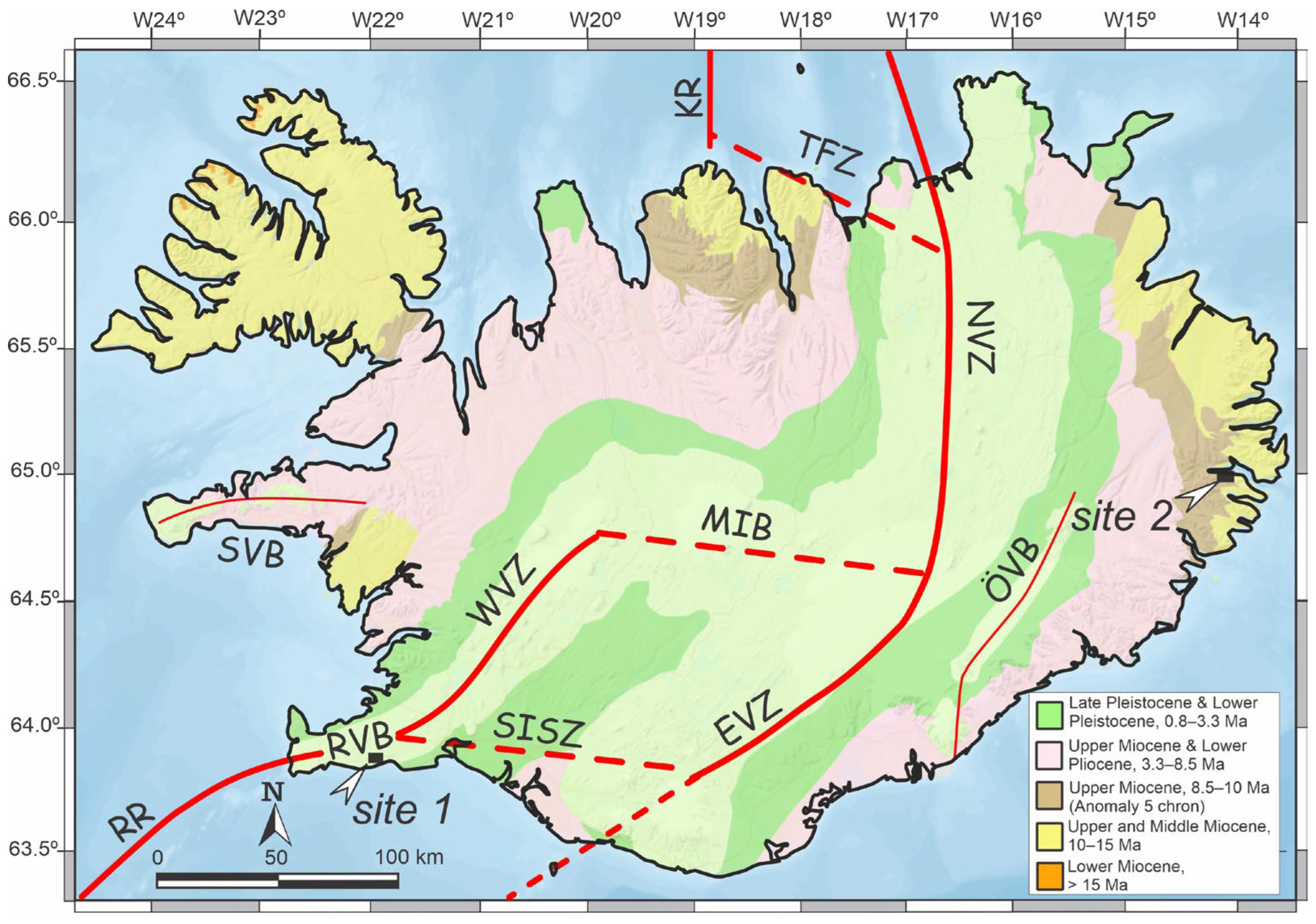
Iceland (Figure 1) provides a unique exposure of a mid-ocean ridge formed by the interaction of the North American and Eurasian plates and the Iceland mantle plume. This has produced a thicker, more complex crust than a typical oceanic crust [19,20]. While deep crustal and mantle studies have examined plume-ridge interactions [21,22], the shallow seismic shear-wave velocity structure—important for understanding seismic hazards—is an emerging research focus.
Volcanic activity in Iceland is concentrated along specific zones where tectonic plates diverge. These zones generally trend from southwest to northeast, following the Mid-Atlantic Ridge, which extends on land as the Reykjanes Volcanic Belt (Figure 1). The volcanic zones are categorised into Rift Zones (where the plates actively pull apart) and Flank Zones (where volcanism occurs just outside the main plate boundaries) [15,16,19,23,24]. Iceland’s geological structure features thick basaltic lavas and hyaloclastites formed by active rifting and volcanic activity [25]. The oldest exposed rocks are only about 16–18 Ma old [23], making the island geologically very young. The crust is categorised into layers based on age and palaeomagnetic patterns [26]. Tertiary flood basalts, mainly subaerial tholeiitic flows with thin clastic beds, cover northwest and east Iceland [27]. These layers dip towards the rift zones, indicating subsidence from crustal loading [28]. The active Neovolcanic Zone is a region of fissure swarms and volcanoes where rifting and magmatism are concentrated [29] and is subdivided into the West, North, and East Volcanic Zones (Figure 1). Seismic velocity models of the Icelandic crust show a rapid increase in velocity with depth within 2–5 km due to pore closure and a mineral transition from zeolite to greenschist facies [30,31,32,33,34,35,36]. Significant lateral differences occur between eroded Tertiary fjord terranes and porous, fractured active rift zones (Figure 1).
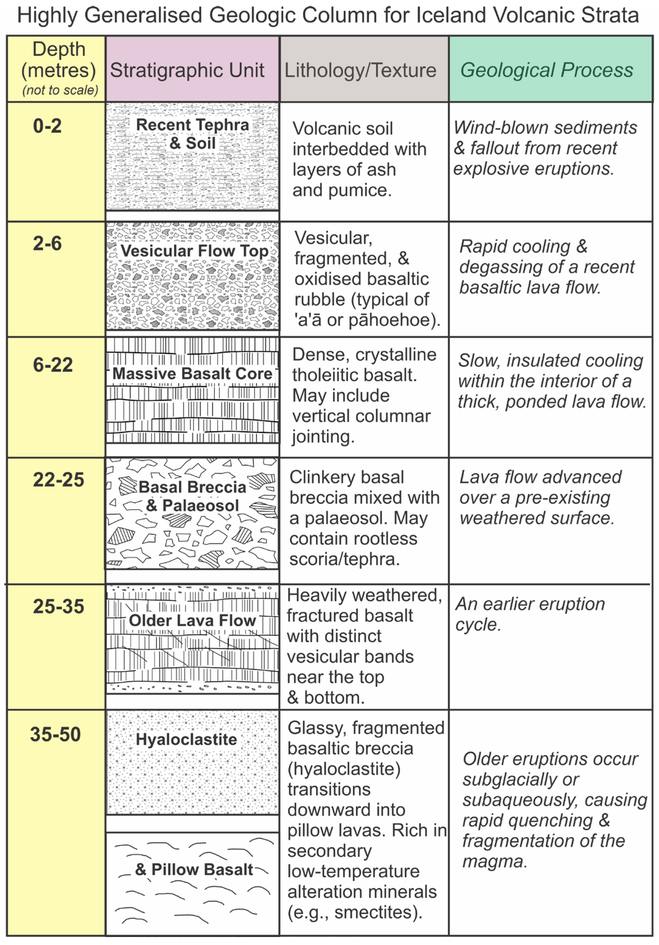
Iceland’s bedrock “layer-cake stratigraphy” (Figure 2) consists of successive basaltic lava flows stacked vertically. Dips typically increase with depth, ranging from near 0° at the Earth’s surface to 5–10° at deeper stratigraphic levels (e.g., at sea level) [37,38]. The basalt flows are often separated by thin sedimentary horizons. Icelandic volcanology distinguishes two primary subaerial basalt flow types: pāhoehoe, with smooth, ropy, or billowy surfaces; and ‘a‘ā flows, with rough, clinkery, and fragmented (“rubble”) surfaces. ‘A‘ā flows often feature a massive core sandwiched between brittle, clinkery top and bottom layers (Figure 2). Transitions between the two flow types are common within a single flow field [37].

3. Previous Near-Surface Geophysical Studies in Iceland

Recent near-surface geophysical studies increasingly aim to characterise shear-wave velocity structure to improve site-effect assessment and soil classification in accordance with Eurocode 8 standards [39,40]. Multichannel Analysis of Surface Waves (MASW) has proven effective for non-invasive profiling of soil and shallow bedrock in Iceland’s complex volcanic regions [41,42]. For example, research in the South Iceland Seismic Zone (SISZ) (Figure 1) has utilised MASW to determine shear-wave velocity profiles as deep as 15–25 m. A foundational study by [41] employed MASW at seven SISZ locations and classified each site according to Eurocode 8. The results showed that sites with sandy glaciofluvial, littoral, or alluvial sediments are assigned to code C, while those with cemented deposits are categorised as B.
A major advancement is the development of nationwide, frequency-dependent seismic site-amplification models. Reference [43] presented nationwide maps of site proxies—including slope, inferred Vs30, and geological units—to refine ground-motion predictions. This work highlights the discrepancy between global amplification models and local Icelandic data, attributing the differences to the country’s young, volcanic geology, for example, by correlating Vs30 with distinct geological units (e.g., lava rock versus sedimentary soil).
To standardise site characterisation, a comprehensive database of measured shear-wave velocity profiles has recently been developed. Reference [42] introduced this open-access resource, which consolidates MASW results from 19 regions across Iceland, tested between 2013 and 2021. The database allows researchers and engineers to view phase-velocity dispersion curves alongside time-averaged shear-wave velocity profiles, making it easier to compare different Icelandic soil types, including gravelly and partly cemented materials that are difficult to sample using traditional borehole methods.

4. Methodologies

While geophysical surveys offer a powerful alternative to direct sampling, individual techniques are often limited by non-uniqueness, depth-resolution trade-offs, or sensitivity to specific physical parameters. For instance, common mid-point (CMP) seismic compressional (P) wave reflection and ground-penetrating radar (GPR) surveys excel at mapping structural boundaries but cannot directly constrain soil or bedrock stiffness (i.e., shear-wave velocity). This study employs a suite of seismic and electromagnetic methods to characterise the subsurface architecture from the near surface down to a stiffer bedrock interface. For two sites, we applied CMP seismic reflection, MASW, and the Horizontal-to-Vertical Spectral Ratio (HVSR) technique; for one site, we applied GPR. We tested several sites in Iceland and selected two, at opposite ends of the island in different geological settings, to illustrate our results. These are the roadcut at the border between Sveitarfélagið Ölfus/Grindavíkurbær along road 427 (site 1) and the southern margin of inner Reyðarfjörður (site 2) (Figure 1).

4.1. Seismic CMP Reflection and MASW Profiles

The seismic reflection data were acquired using a static geophone spread (‘walk-through’) with 48 recording channels and processed as a short CMP reflection profile, and as active- and passive-recorded MASW input to produce a one-dimensional shear-wave velocity profile (using ParkSEIS© Version 3.0 [44]). The CMP data were used to obtain a stacked profile of reflections from volcanic strata for comparison with the MASW results, with the midpoint of the resulting Vs model located at the approximate centre of the CMP profile. For the MASW surveys, no acquisition filters were used. For each site, several survey strategies were tested: the source-to-nearest-receiver distance was varied (1–25 m) for active-source recordings; passive-source recordings were made by listening for 30 s (sample rate = 2 ms) and 60 s (sample rate = 4 ms), with six records stacked. Rayleigh-wave dispersion spectra for shear-wave velocity inversion were generated [6] and compared with the CMP profiles.
The geophone CMP array length was 47 m at site 1 and 70.5 m at site 2 (Figure 1). All surveys used 4.5 Hz geophones. The CMP surveys used a field acquisition filter of 10–1000 Hz to reduce surface-wave energy. The seismic source was a sledgehammer (4–6 kg) struck against an aluminium plate, stacked four or five times to reduce random noise. The CMP profiles had a maximum fold of cover of 48. The data processing steps [45] consisted of assigning three-dimensional station geometry, top muting of linear arrivals (direct arrival and head waves) and bottom muting of surface-wave energy, Ormsby frequency bandpass filtering (30–40–400–500 Hz, trapezoidal), automatic gain control (200 ms window), CMP sorting, CMP stretch mute (attenuation of any sample moved in time by 30% or more) to further suppress first breaks (direct and head waves), normal moveout (NMO) velocity analysis and application for CMP stacking and to derive a simple root-mean-square (RMS) velocity for time-to-depth conversion, stacking of CMP-sorted traces, phase-shift migration, depth conversion, and display. We also experimented with post-stack seismic attribute displays to aid interpretation [46], with reflection strength being most useful. Further processing details are provided in Section 5: Results and Interpretation.
At site 1, there was no appreciable elevation difference along the survey. The Reyðarfjörður site 2 required an elevation static correction (datum is the highest elevation above mean sea level along the profile, 40 m, with a replacement velocity of 2500 m/s). Deconvolution filtering [45] was tested but deemed destructive given the complexity of the reflectivity series. Multiple reflected arrivals were not apparent in the shot records or on the CMP stack sections. For site 1, the minimum vertical resolution, estimated using the Rayleigh criterion, is 2 m (using a compressional wave velocity of 400 m/s, derived from RMS velocity analysis, and a minimum dominant frequency of 50 Hz). For site 2, the minimum vertical resolution, estimated using the Rayleigh criterion, is 5 m (using a compressional wave velocity of 1000 m/s, derived from RMS velocity analysis, and a minimum dominant frequency of 50 Hz).

4.2. HVSR Soundings

The Horizontal-to-Vertical Spectral Ratio (HVSR) method, also known as the Nakamura method, is widely used in site investigations to estimate the resonant frequency of soft layers overlying hard bedrock (e.g., depth < 50 m) [47,48,49,50,51,52,53]. The technique relies on the ratio of the amplitude spectra of the horizontal (H) and vertical (V) components. Peaks in the HVSR curve typically indicate resonant frequencies at which soft materials amplify ambient vibrations caused by wind, ocean waves, traffic, or footsteps [51,52,53]. Natural vibrations generally occur at low frequencies (e.g., <1 Hz), whereas human-made or very shallow sources tend to generate higher-frequency components (e.g., >1 Hz). The method uses a small, three-component seismometer to measure passive ground vibrations, making it adaptable to nearly any location [54,55,56]. The HVSR technique has been used to derive site shear-wave velocity (Vs) profiles for engineering purposes, including evaluating ground-shaking amplification [57,58,59]. It has also been applied to characterise sedimentary cover and to determine the depth to the underlying bedrock [59,60,61,62].

4.3. 3D GPR Survey

GPR (ground-penetrating radar) provides higher resolution than seismic or other geophysical methods and detects rock-property changes at scales as fine as decimetres [63]. For sites where chemical weathering has not progressed to high clay content and where ground conditions are dry, volcanic deposits can make excellent radar targets. The ability of georadar to image the internal structure of volcanic deposits also depends on the variability in porosity within the deposits (i.e., variation between air and matrix). Site 1 was also ideal for a GPR survey because it lies directly above a roadcut, which was used to support the geophysical interpretation.
A three-dimensional (3D) GPR survey was conducted just above the roadcut, along a smooth, graded road with thin asphalt paving (area = 5 m × 67.6 m). A 120 m-long two-dimensional (2D) profile was collected through the centre of the 3D survey to provide context. The survey was carried out during a dry period using a GSSI (Geophysical Survey Systems, Inc, Nashua, NH, USA.) bistatic 400 MHz antenna with a field-frequency filter set to 100–800 MHz. Data were recorded as individual 2D profiles, spaced 25 cm, using a distance wheel, with a sample rate of 2048 samples per trace (~0.1 ns per sample), 36 traces per metre, and a record length of 200 ns. Because the GPR survey was conducted over mostly flat ground, no topographic correction survey was necessary. Processing the 2D georadar data began with an exponential amplitude gain function, followed by ‘background’ removal based on continuity across 199 traces (a typical value) to eliminate direct arrivals, ground-borne arrivals (e.g., refractions), and radar ring-down effects [64,65]. An automatic gain control (AGC) was applied to balance low and high amplitudes [56]. Kirchhoff migration [66] correctly repositioned dipping reflections. The velocity of the electromagnetic signal transmission was determined via diffraction modelling. We also calculated seismic attributes [46] for the profiles to guide interpretation. The vertical resolution, estimated using the Rayleigh criterion, is about 7 cm (based on a centre frequency of 400 MHz and an electromagnetic propagation velocity of 0.1058 m/ns, derived from diffraction modelling, see below).

5. Results and Interpretation

5.1. Sveitarfélagið Ölfus/Grindavíkurbær Roadcut

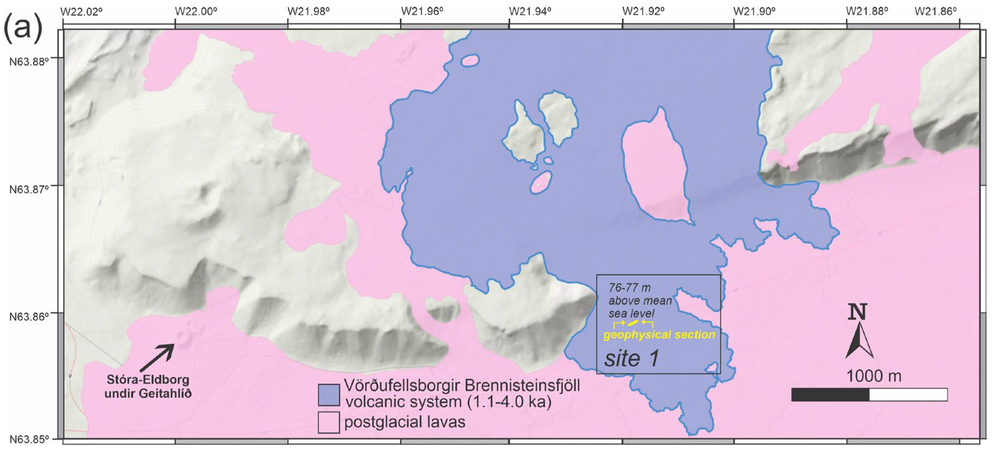
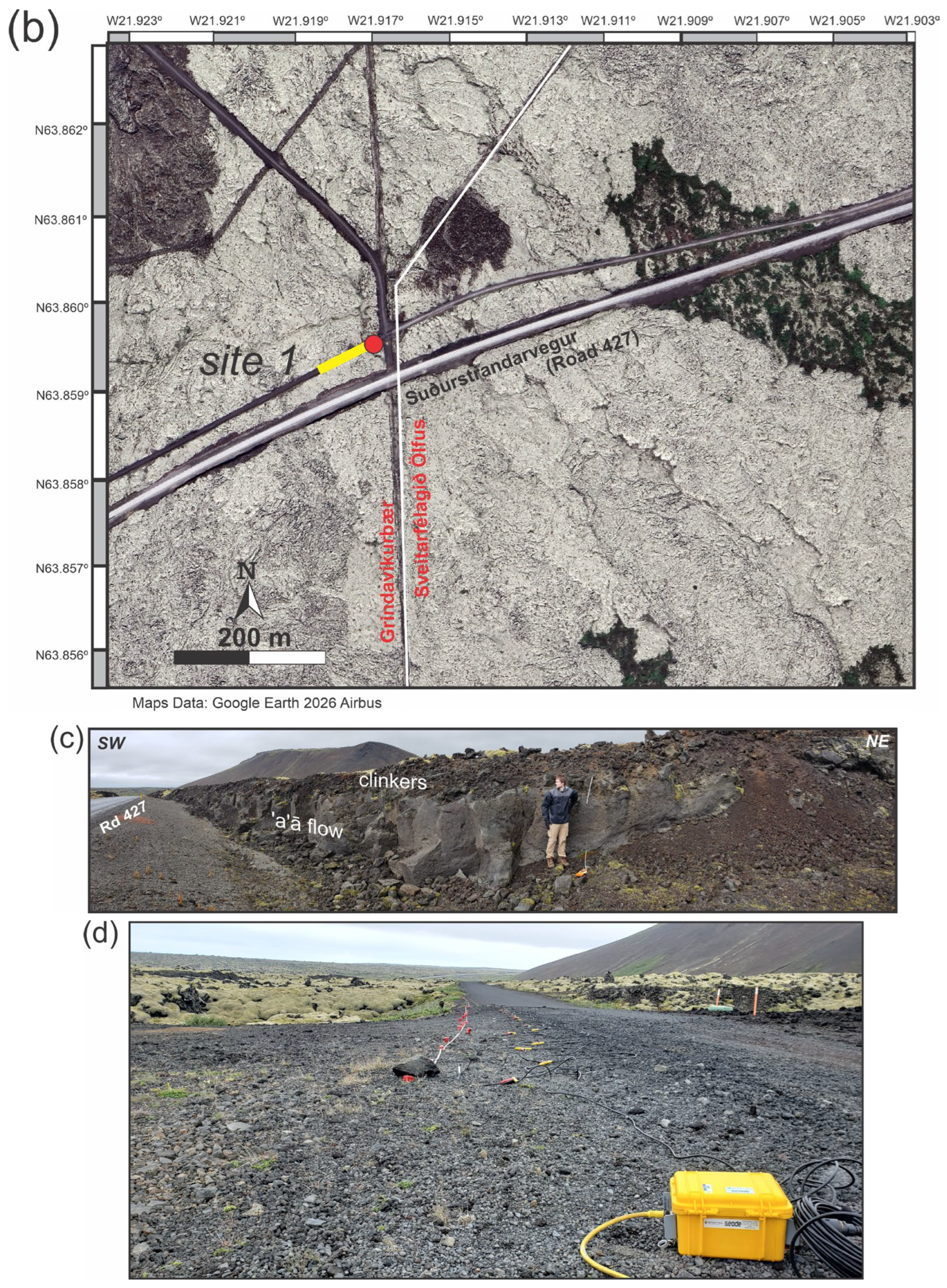
The road 427 cut site 1 is located just west of the Sveitarfélagið Ölfus/Grindavíkurbær border (Figure 3a–d) on the easternmost edge of Suðurnes. The local geology consists of Holocene-to-Prehistoric mafic and intermediate lavas, part of the tholeiitic Brennisteinsfjöll volcanic system, dating to 1100–4000 years before present [23]. The lavas around the survey site are generally not heavily eroded, though they may be weathered and vegetated.

5.1.1. CMP Seismic Reflection

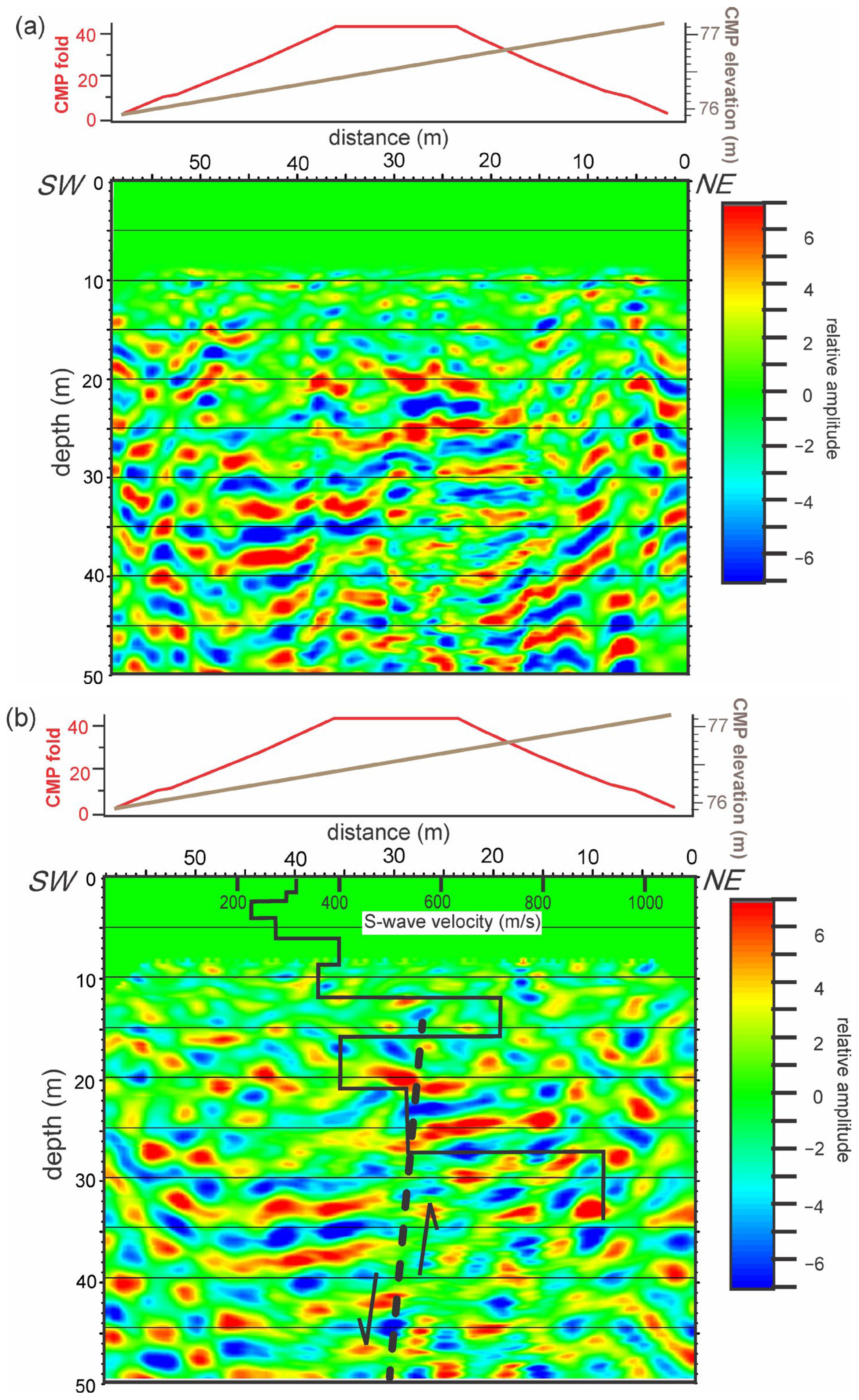
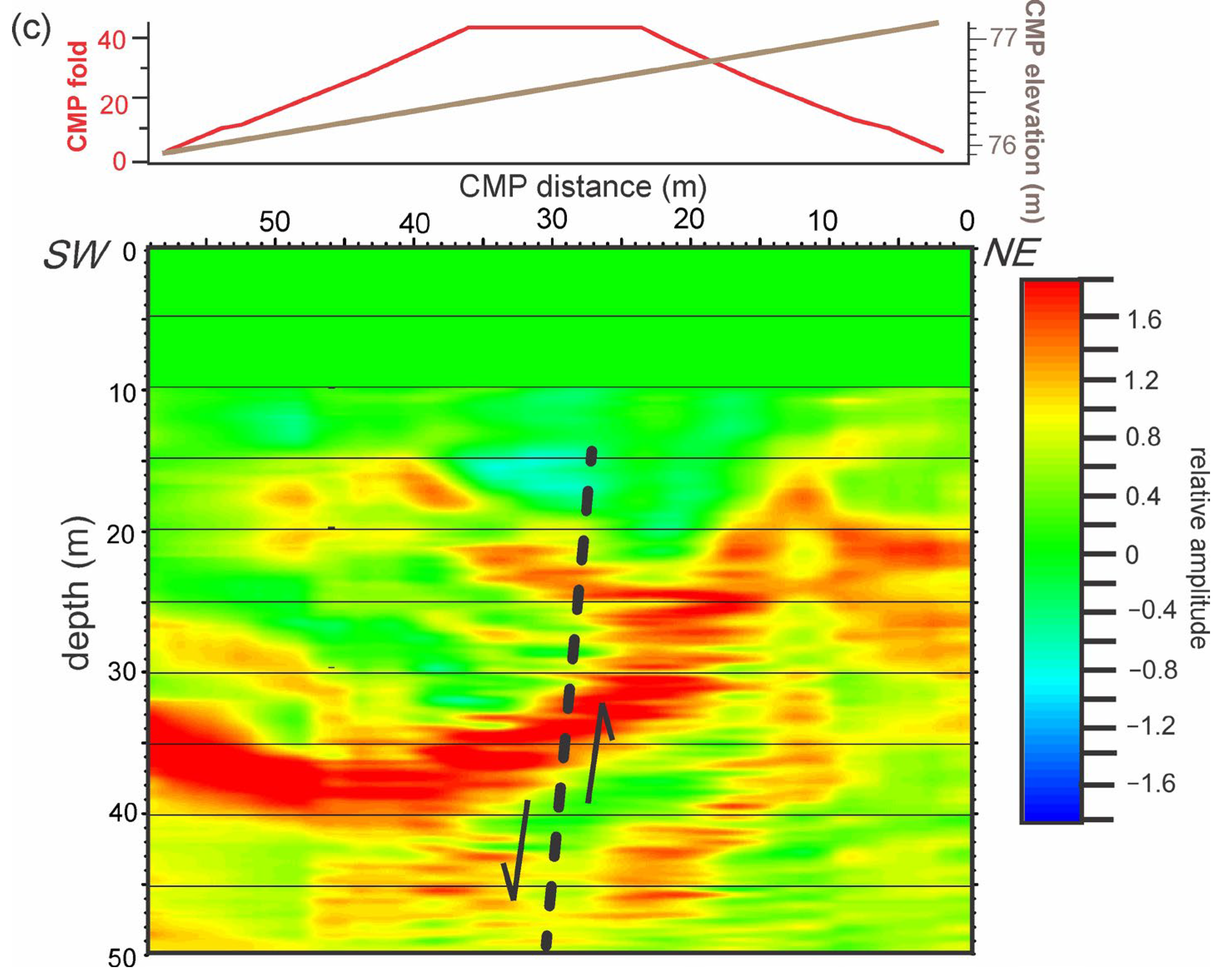
The CMP-stacked P-wave section is shown unmigrated (Figure 4a), migrated with interpretation (Figure 4b), and as reflection strength (Figure 4c). To mitigate potential contamination from first-break and surface-wave arrivals stacked with reflections, the upper part of the field records was aggressively muted at the top and bottom, as well as by CMP stretch muting. Both the unmigrated and migrated sections show an offset reflection between 25 and 33 m depth (about 8 m vertical offset) within the horizontal distance range 15–45 m. The offset is interpreted as a near-vertical or steeply west-dipping (in the plane of the section) normal fault. The reflection-strength seismic attribute envelope (Figure 4c) isolates the highest-amplitude events, supporting the observation of a reflector offset.

5.1.2. MASW

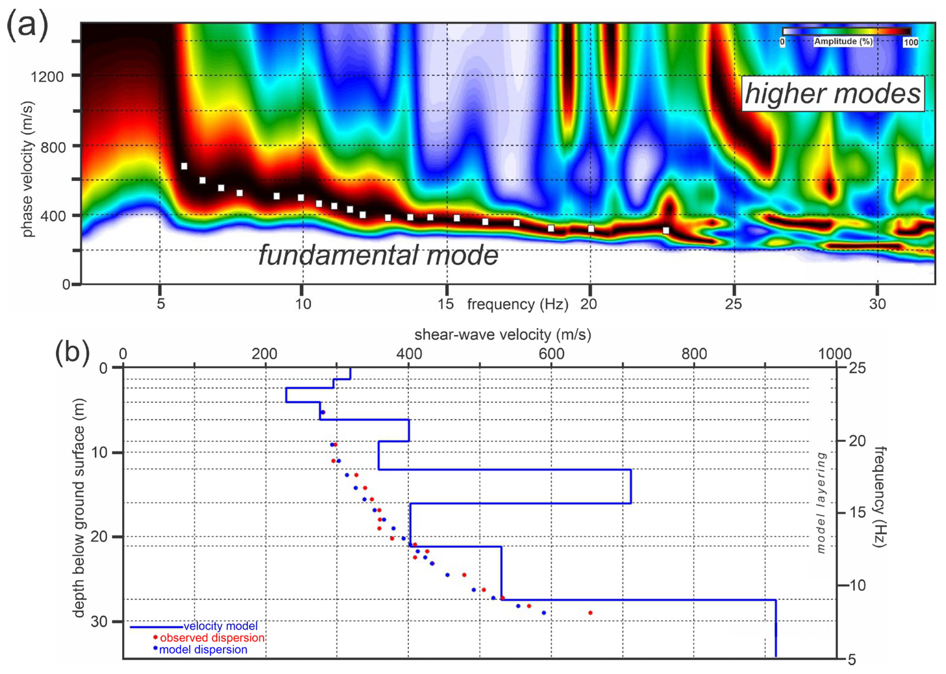
For the MASW recordings, six 60 s passive records were processed and their respective dispersion images stacked, producing a dispersion spectrum (Figure 5a) with a high-amplitude response between about 5 Hz, just above the geophone resonant frequency, and just below 25 Hz. Over this frequency interval, the phase velocities ranged from 1000 m/s to 200 m/s. The fundamental mode dispersion function was extracted to produce the Vs-depth model shown in Figure 5b. The model shows a variable, low-Vs upper layer (250–315 m/s), 3–4 m thick, interpreted as loose clinker material at the top of an ‘a‘ā flow (Figure 3c), with an underlying core with variable Vs = 400–710 m/s. The velocity inversion between 16 m and 20 m could represent clinker or other loose material at the base of the flow(s), which is then underlain by higher-Vs material. The Vs30 derived from the Vs model is 421 m/s, which corresponds to Eurocode Ground Type B [4] or NEHRP Seismic Site Class C (‘very dense soil and soft rock’) [5]. Superimposing the Vs-depth model on the migrated CMP section (Figure 4b) indicates that the upper limit of the onset of coherent P-wave reflectivity (~16 m depth) corresponds to the first prominent inversion on the Vs model (Figure 5b), underlain by a jump to 530 m/s at 21 m depth and then again deeper to 910 m/s at about 27 m. The velocity inversion (16–21 m depth) could represent a zone of fracturing or brecciation associated with the emplacement of the ‘a‘ā flow (Figure 2).

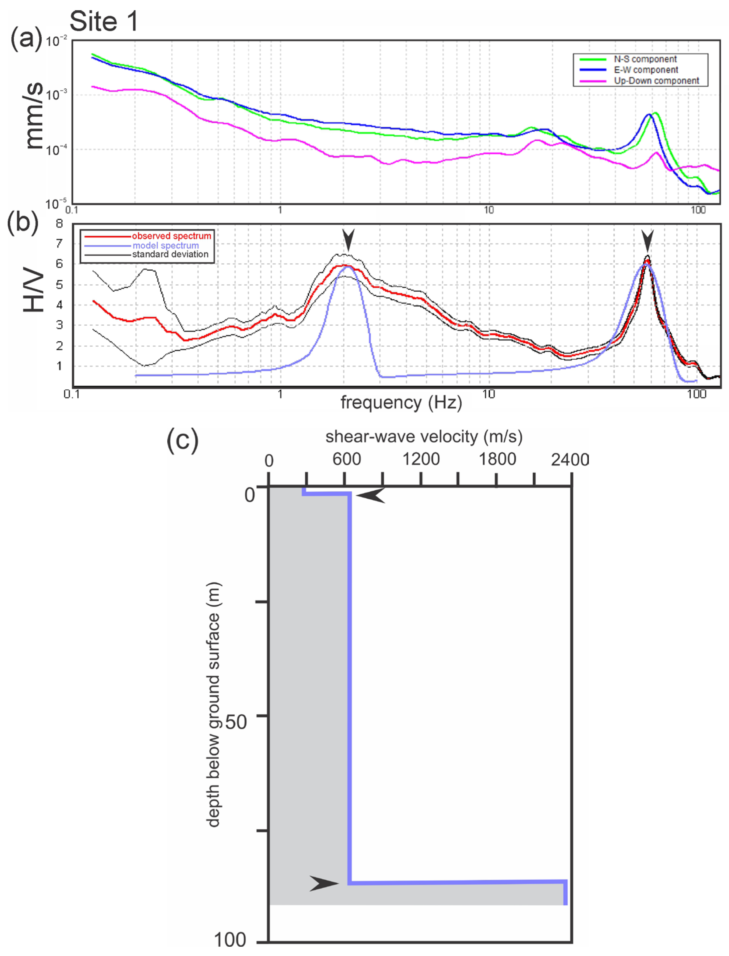
5.1.3. HVSR

To model the H/V spectra (Figure 6a), the thicknesses and Vs values of the upper and lower layers were adjusted to match peak position and amplitude, starting with Vs = 240 m/s for the HVSR model (Figure 6b,c), which approximately matches the averaged Vs from the uppermost layers in the MASW model (Figure 5b). The H/V frequency spectra (Figure 6a) can be modelled (Figure 6b) with two prominent subsurface boundaries: (1) a shallow (1.3 m) interface interpreted to lie between a surface clinker layer and the dense core of an ‘a‘ā flow (Figure 6c); (2) a deep interface at 85 m (Figure 6c), above which we interpreted the layer to represent the core of the ‘a‘ā flow (Figure 2). The shallow interface is at about one-third the depth of the uppermost low-Vs layer modelled from the MASW data (Figure 5b). The middle interval’s velocity in the HVSR model is a little over 600 m/s (Figure 6c), which is considerably greater than the averaged Vs for the upper 30 m from the MASW velocity model (Vs30 = 421 m/s, Figure 5b); however, the upper 30 m-thick interval in the lower-resolution HVSR Vs model represents part of the composite average of the entire HVSR 85 m thick interval, meaning that the two velocities would not be expected to be equivalent. Note that the HVSR model (Figure 5) complements the MASW Vs model (Figure 5b) and the CMP profile (Figure 4a), both of which are unable to detect targets below 30–50 m.
When comparing MASW with HVSR, reasonably coherent results were obtained. Both methods detect a boundary between surface clinkers and a dense ‘a‘ā core, although the clinker layer as modelled by MASW is more complex than in the HVSR model. HVSR has the advantage of detecting deeper boundaries than MASW. The boundary at 85 m (Figure 6c) is undetectable by MASW, suggesting that it is advantageous to deploy both methods at any given site. MASW can provide important velocity inputs, especially the upper-layer Vs, to guide HVSR modelling, whereas HVSR can detect deeper features.

5.1.4. GPR

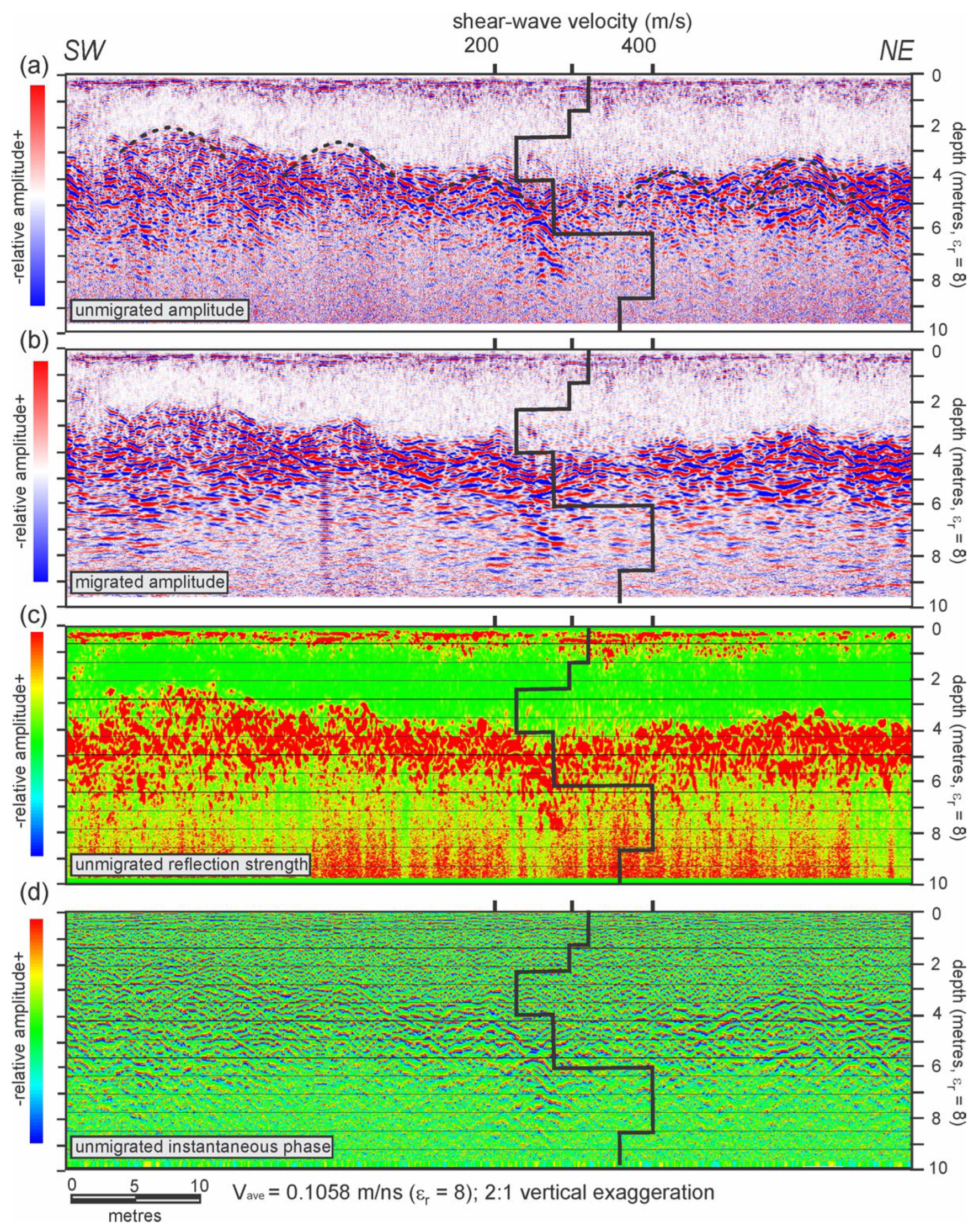
We surveyed a ~120 m-long GPR 2D profile along the CMP and MASW lines, where elevation changes were negligible. The ground conditions at the time of the survey were moist. A time-to-depth conversion, obtained by fitting hyperbolae to diffractions on the unmigrated profile (Figure 7a), yielded an average velocity of 0.1058 m/ns (equivalent to a dielectric constant of 8), consistent with previous studies of basalt dielectric constants under wet conditions [67,68]. The migrated amplitude profile (Figure 7b) shows a transparent zone that varies in thickness from 2.3 to 4.7 m below the acquisition surface. Beneath this layer lies a strongly reflective (highly scattering) zone (Figure 7c,d) with numerous overlapping diffractions and dipping reflections. Due to the complexity of the scattering surface, including likely out-of-plane arrivals, the migration was performed with a reduced average velocity to suppress over-migration artefacts. The internal structure of the 2–4 m-thick reflective zone shows a sparse stratigraphy of short reflection segments, 1–3 m long, together with collapsed diffractions, reflecting the jagged, chaotic nature of the lava emplacement, such as might be expected from an ‘a‘ā flow (Figure 2).
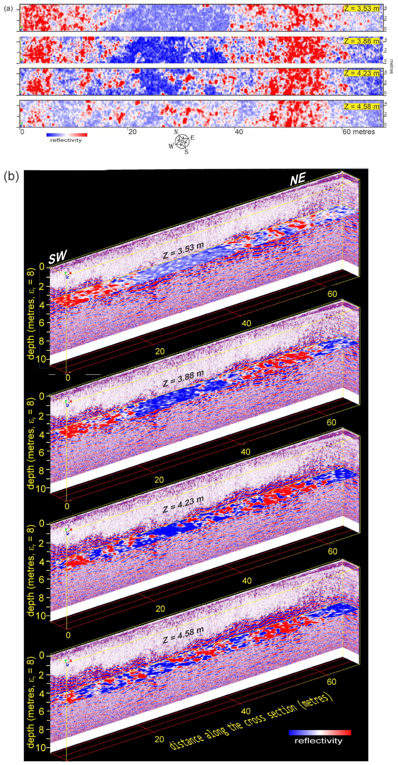
In general, ‘a‘ā basalt flows are characterised by a highly structured three-part internal architecture, typically comprising a rough, brecciated upper clinker layer, a massive, dense and finely crystalline core, and a thinner basal breccia or vesicular zone (Figure 2). The roadcut (Figure 3d) exposes the massive core and the associated ‘a‘ā stratigraphy (Figure 2). The upper transparent zone in the radar data, interpreted as the upper clinker layer or its eroded products, approximately corresponds to the uppermost low-Vs zone in the MASW-derived model (i.e., the top of the radar reflective zone matches the base of the Vs inversion, Figure 5b). Our results are consistent with previous GPR studies of ‘a‘ā flows [67,68]. Horizontal depth slices through the 3D GPR volume (Figure 8a,b) reveal the uneven, corrugated nature of the reflective zone, with elevation relief up to about 2.5 m.

5.2. Reyðarfjörður

Our study site in eastern Iceland lies along the southern margin of inner Reyðarfjörður, the longest and widest fjord in eastern Iceland. The bedrock exposed along the fjords of eastern Iceland (Austfirðir) (Figure 9a–d) consists of mafic and intermediate extrusive Lower Pliocene and Miocene rocks intercalated with red-coloured sediments, originally soil horizons (all older than 3.3 Ma; 10–15 Ma [23,69]) (Figure 2). Due to loading in the volcanic zones west of Austfirðir, the lava beds cropping out along the fjords typically dip west towards the volcanic zone. Pleistocene glaciers subsequently carved deep valleys and fjords into the bedrock [23].

5.2.1. CMP Seismic Reflection

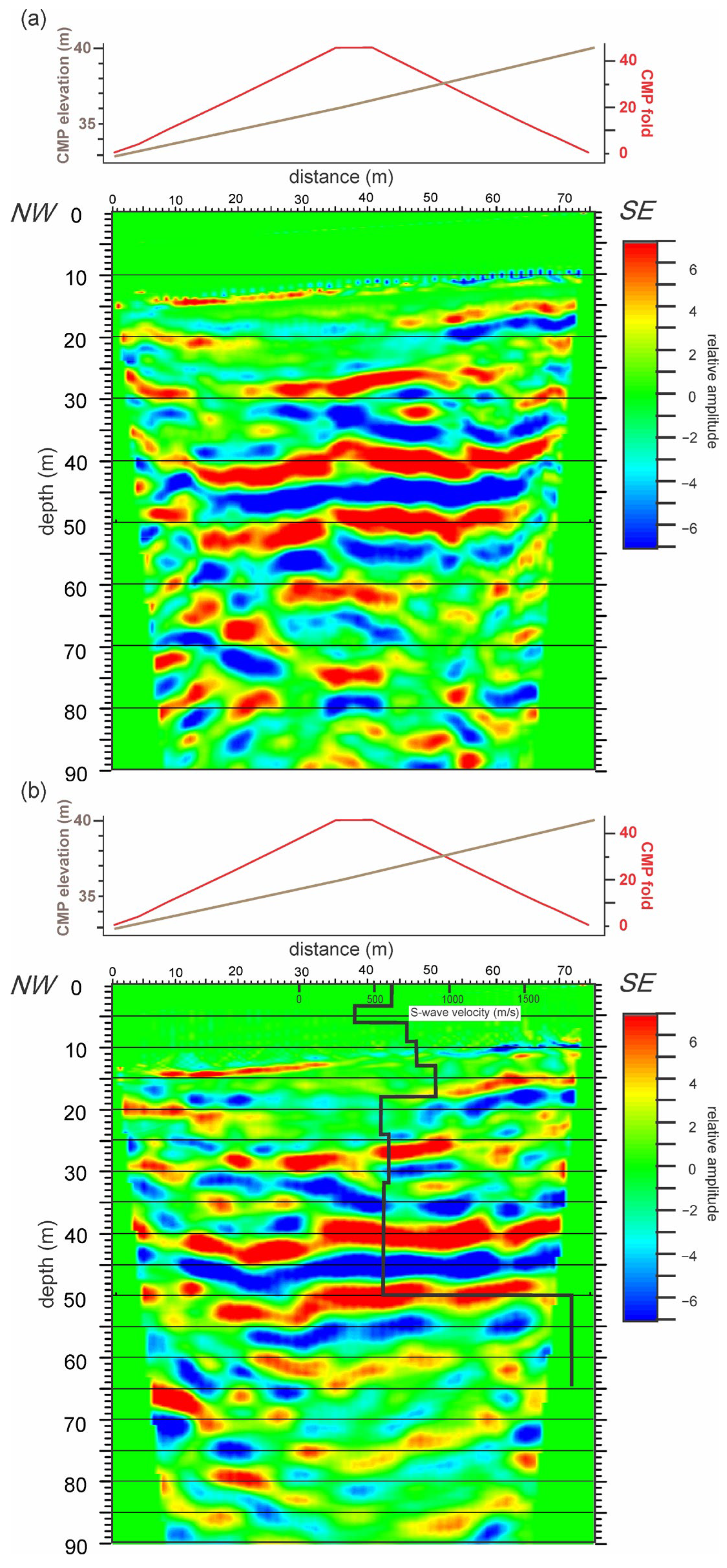
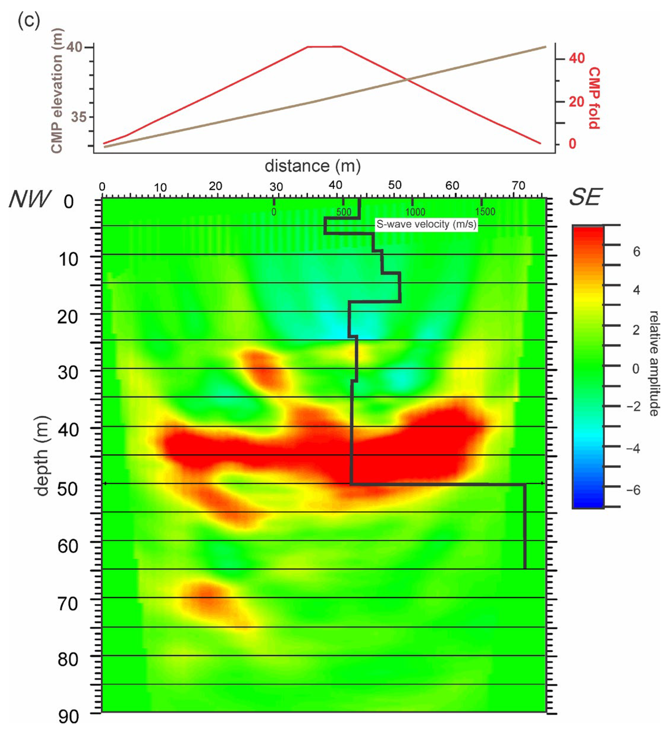
Following the format of site 1, the CMP-stacked P-wave section is shown unmigrated (Figure 10a), migrated with interpretation (Figure 10b), and as reflection strength (Figure 10c). To prevent contamination from first-break and surface-wave arrivals mixing with reflections, the upper section was extensively muted at the top and bottom, along with CMP-stretch muting. Both the unmigrated and migrated sections show a layered reflectivity structure in the upper 50–60 m (Figure 10a,b), particularly between 3 and 55 m depth. The reflection-strength seismic attribute envelope (Figure 10c) isolates the highest-amplitude events at depths between 35 and 55 m. The dip of the reflectors varies between 5° and 10° west (in the plane of the section), which matches the outcrop observations (Figure 9a) and reports on the dip of volcanic beds along the coast in the Reyðarfjörður area [23,27].
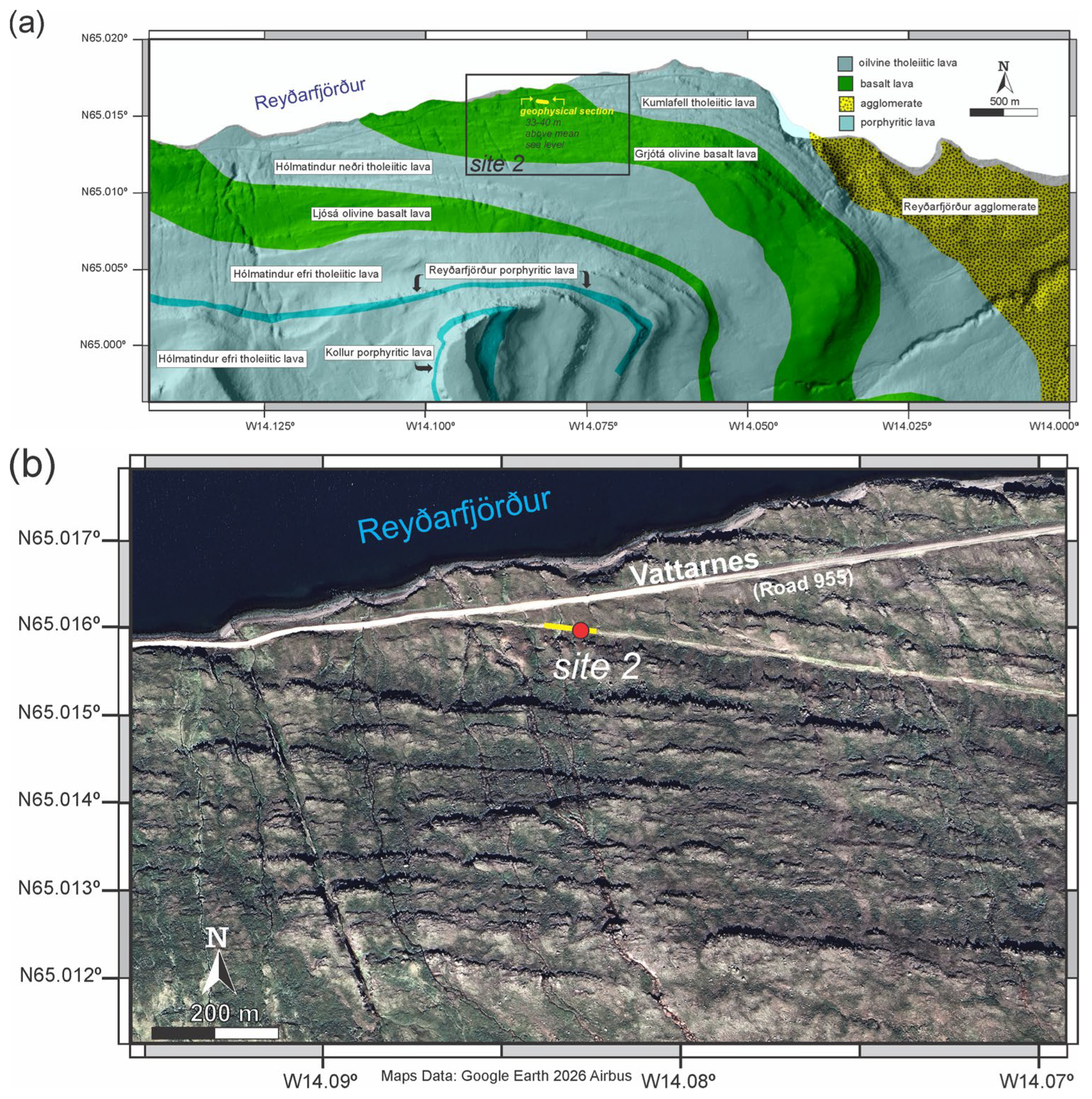
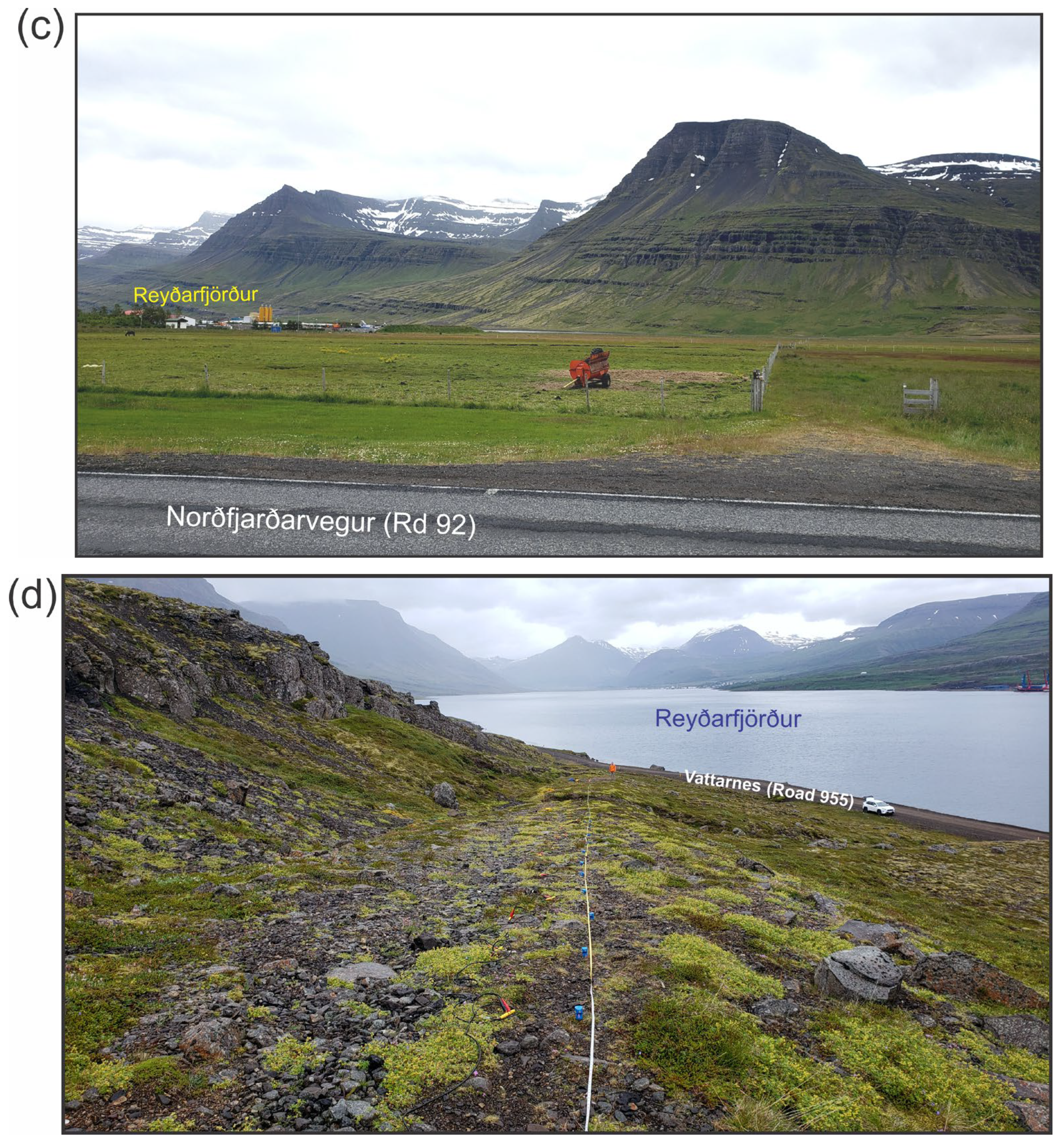
Figure 9. (a) Site 2 (Figure 1) shaded relief map with Miocene-age geologic units. Source of information: [23]. “Reyðarfjörður” refers to the fjord north of site 2. (b) Google Earth satellite image of site 2 in (a). “Vattarnes” refers to the name of the road that passes by site 2. The yellow line is the area of seismic surveys. The red dot is the location of the HVSR sounding. Note the prominent ridges of volcanic rock outcrop. (c) Photo (by J. McBride) just west of the town of Reyðarfjörður, looking approximately south, 8 km west of site 2 (b). “Norðfjarðarvegur” refers to the name of the road along which the photograph was taken. Location of the photographer: 65.032627° N, 14.247164° W. Note well-developed volcanic outcrop ridges, like the location of site 2 (b). (d) Photo (by J. McBride) looking west along the trail where the geophysical surveys were located (yellow line in (b)). Location of the photographer: 65.015943° N, 14.081423° W.
Geohazards 07 00085 g009aGeohazards 07 00085 g009b
Figure 10. (a) P-wave CMP unmigrated reflection profile from Site 2, displayed with no vertical exaggeration. See Figure 9b for location. (b) Same as above but migrated and shown with the corresponding S-wave velocity function from MASW superimposed (Figure 11b). (c) Same as above but processed as relative reflection strength.
Geohazards 07 00085 g010aGeohazards 07 00085 g010b
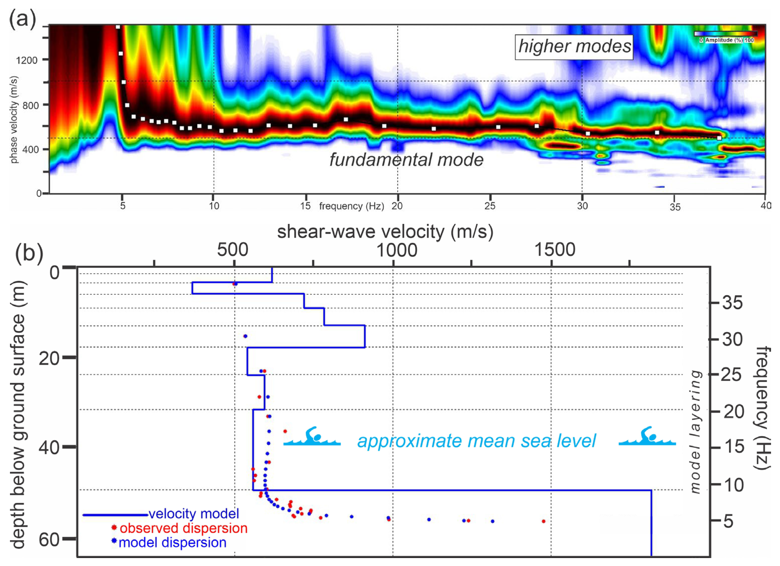
Figure 11. (a) Phase-velocity frequency spectrum for site 2, derived from the 60 s passive recording. White squares (connected by thin black line) are the dispersion function used for shear-wave velocity inversion (b). (b) Shear-wave velocity model based on inversion of the dispersion function (a).
Geohazards 07 00085 g011

5.2.2. MASW

As with the previous site, six 60 s passive records were processed from the MASW recordings, and their respective dispersion images were stacked. The dispersion spectrum (Figure 11a) shows a high-amplitude response between about 5 Hz, just above the geophone resonant frequency, and 38 Hz. The phase velocities over this frequency interval ranged from 1500 m/s to 500 m/s (Figure 11a). The extracted fundamental-mode dispersion function yields a model that shows an upper low-Vs layer starting at the ground surface at 625 m/s, ~3 thick, followed by a velocity inversion (~400 m/s), 2–3 m thick, interpreted as rubbly and weathered zones on top of more indurated volcanic layers (Figure 9d), underlain by a 13 m thick higher-velocity zone with a variable Vs = 730–925 m/s, in turn overlying a ~32 m thick more homogeneous layer with a Vs of 565 m/s–620 m/s. The base of the Vs model lies at a depth of 50 m, with a half-space velocity of about 1800 m/s. The Vs30 derived from the Vs model is 617 m/s, which corresponds to Eurocode Ground Type B or NEHRP Seismic Site Class C (‘very dense soil and soft rock’).
Superimposing the Vs-depth model on the migrated CMP section (Figure 10b) indicates that the upper limit of the onset of P-wave layered reflectivity (~20 m depth) coincides with the first prominent inversion in the Vs model (Figure 10b). The reflective interval from 20 m to about 50 m depth on the P-wave CMP section (Figure 10b) corresponds to the low S-wave velocity zone (Figure 11b). The base of this zone on the Vs-depth model (Figure 11b) matches the base of the P-wave reflective zone (Figure 10b,c).

5.2.3. HVSR

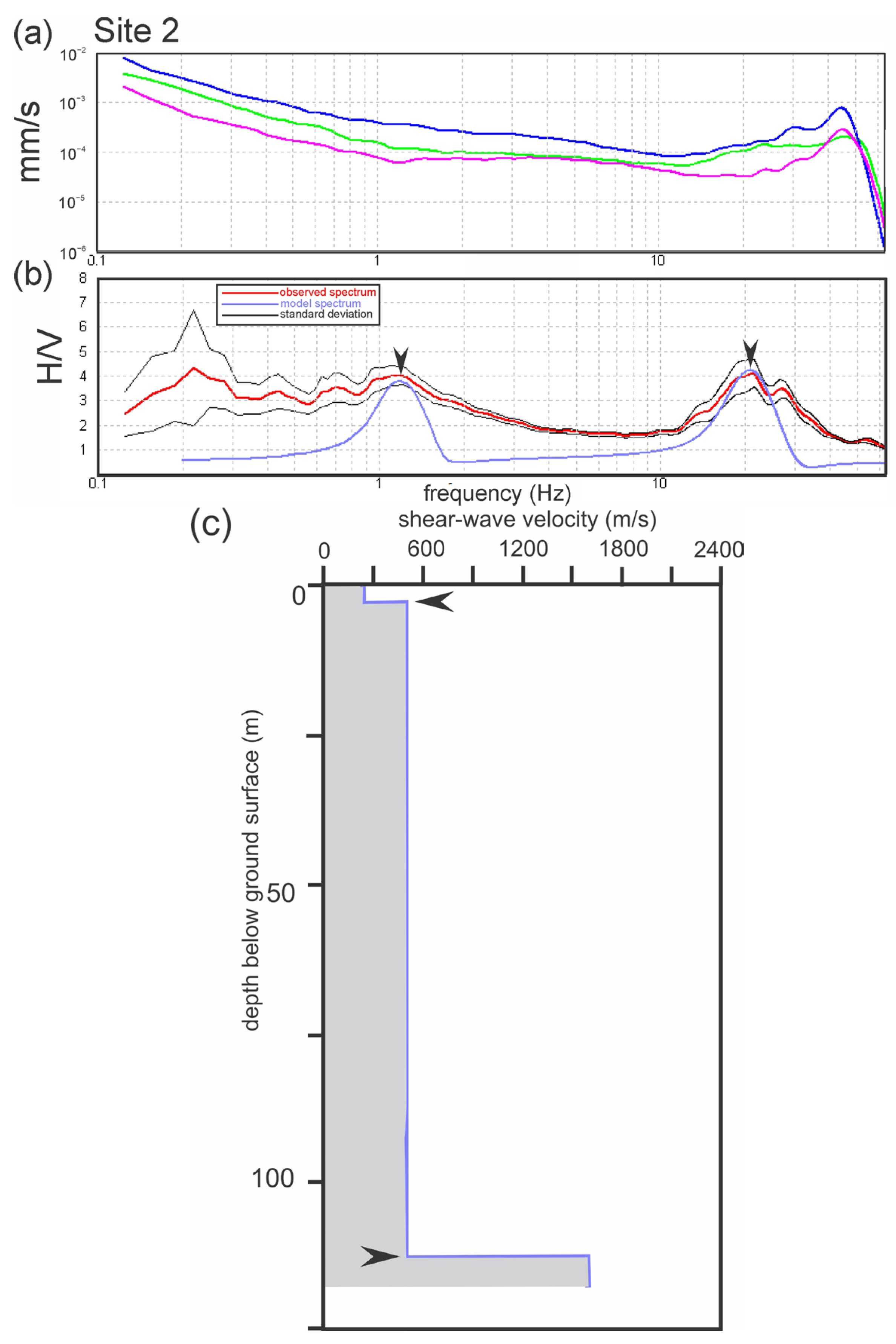
As with the HVSR model for site 1 (Figure 6a–c), the H/V frequency spectra (Figure 12a) can be modelled (Figure 12b,c) with two prominent subsurface boundaries: (1) a shallow (~3 m) interface interpreted to lie between a weathered and rubbly zone starting at the ground surface (Figure 9d); (2) a deep interface at 110 m (Figure 12c) overlying a middle layer with Vs = 500 m/s, which corresponds to the layered P-wave reflectivity on the CMP section (Figure 10b). The shallow interface is at about the same depth as the uppermost low-Vs layer modelled from the MASW data (~3 m, Figure 11b). The velocity of the middle interval in the HVSR model (Vs = 500 m/s) (Figure 12b) is considerably less than the averaged Vs for the upper 30 m from the MASW velocity model (617 m/s, Figure 11b); however, as was the case for site 1, the upper 30 m-thick interval in the lower-resolution HVSR Vs model, represents only part of the composite average of the entire HVSR 115 m thick interval—the fact that the Vs of the middle HVSR model layer is less than the Vs30 of 617 m/s may reflect the greater degree of chemical weathering at depth, expected for the much older volcanic strata in Austfirðir (site 2) as opposed to Suðurnes (site 1) (Figure 1).

5.2.4. MASW of Scholte Waves

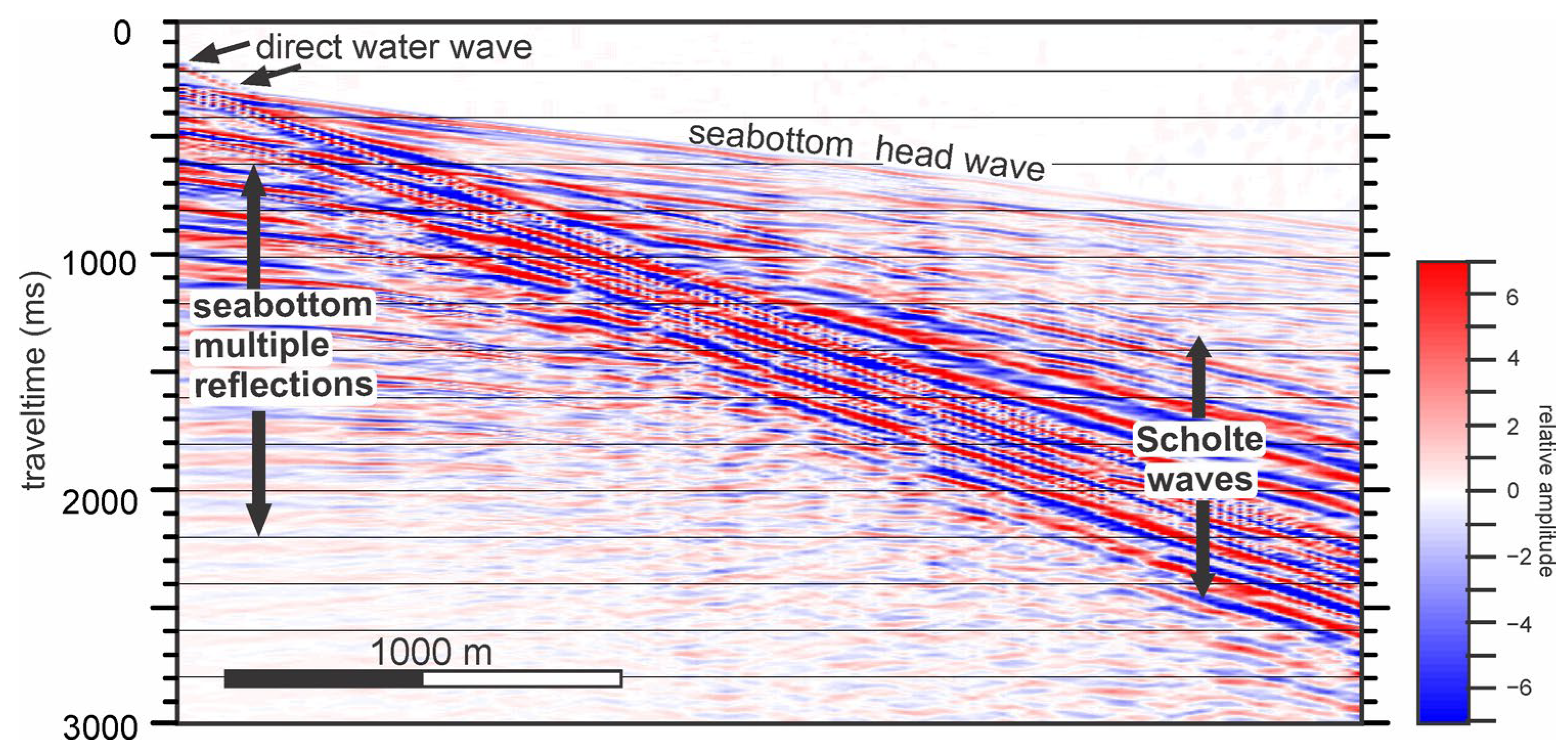
We take advantage of the fortuitous availability of marine common-source P-wave seismic data recorded in 1994 for a long-record CMP profile by the British Institutions Reflection Profiling Syndicate (BIRPS) [70,71,72] (Figure 9a,b). We selected one record (Figure 13), the closest to our study site (about 8 km offshore to the northeast) (Figure 9a,b). The energy source was a large 36-element airgun array (153 litres) towed from the vessel’s stern at 10 m depth. The hydrophone streamer was at a depth of 18 m. The distance from the centre of the airgun array to the first hydrophone group was 247.5 m. The hydrophone group interval was 25 m, with 48 individual hydrophones per group. The streamer length was about 3000 m, with 120 recording channels. Total recording time was 27 s. Due to the relatively hard seafloor (Vs > VP of water, i.e., Vs ≥ 1500 m/s) [73] and the source and recording parameters, conditions were suitable for the generation of Scholte waves.
Scholte waves are specialised seismic interface waves that propagate along the boundary between a fluid layer, such as seawater, and a solid elastic medium, such as the seafloor [74,75]. Their particle motion and dispersive properties closely resemble those of Rayleigh waves on land, making them useful for underwater MASW analysis of the Vs structure beneath the seafloor [76]. Furthermore, the unusually long receiver cable (relative to high-resolution MASW land surveys) and the very large energy source act together to significantly increase the depth of investigation compared with conventional MASW [77].
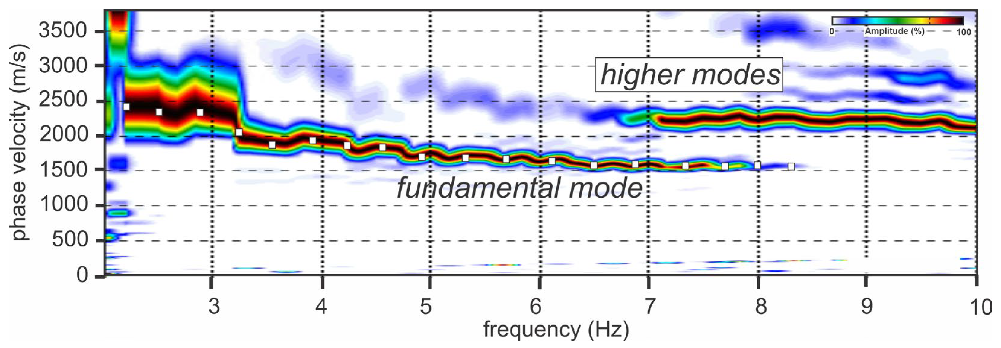
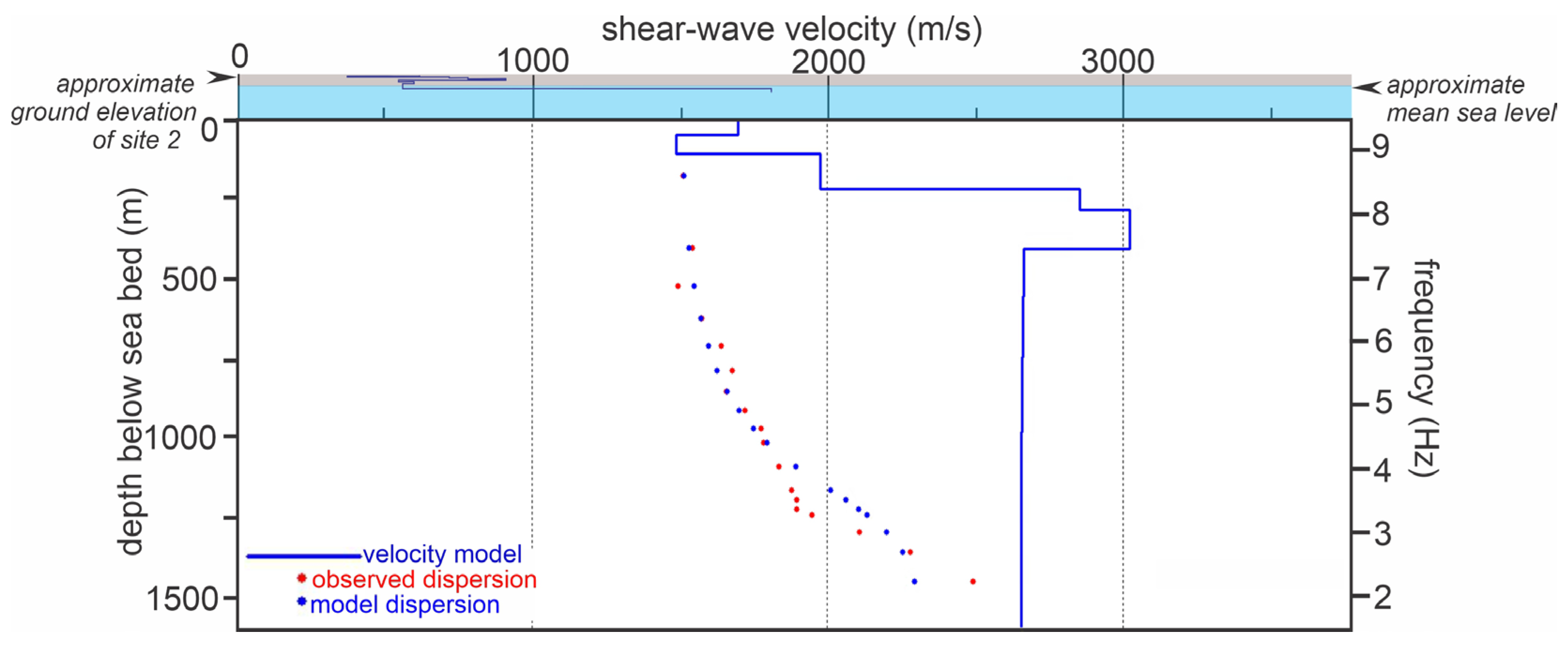
For the MASW of the offshore records, we use the same inversion approach as applied to the two previous onshore sites. The Scholte wave modelling assumes that the data were collected using seabed receivers [73]. The dispersion analysis yielded a high-quality phase-velocity-frequency spectrum (Figure 14), showing a well-developed fundamental mode (2–8 Hz) and higher modes (7–15 Hz). For this study, we analysed only the fundamental mode. Phase velocities ranged from 1500 to 3000 m/s. The modelling results (Figure 15) span the frequency range of 2–9 Hz and provide a Vs-depth profile starting with a 50 m-thick layer at about 1700 m/s, underlain by an inversion to about 1480 m/s. The Vs model then jumps to about 1980 m/s at 100 m depth, below which the velocity increases to a maximum of just over 3000 m/s. Finally, the velocity inverts to 2690 m/s at about 400 m depth, down to the maximum depth of investigation at about 1500 m. Weathered basalt can have a Vs of 100–1500 m/s [78,79], whereas compact and massive basalt in the deep crust can have a Vs of 2200–3800 m/s [79,80]. These values are consistent with the results of our model [79,80].

6. Discussion

While our study builds on foundational research by Icelandic geophysicists and engineers to precisely identify and map subsurface geological hazards [18,39,41,42,43], the integrated, multi-method workflow developed here can serve as a template for characterising shallow basalt stratigraphy more broadly. Through experimental surveys, we utilised complementary geophysical techniques to explicitly characterise the shallow subsurface. Specifically, we built robust geological models for two study sites by integrating structural imaging—using P-wave Common Midpoint (CMP) and 3D Ground Penetrating Radar (GPR)—with shear-wave velocity data extracted from Multichannel Analysis of Surface Waves (MASW) and Horizontal-to-Vertical Spectral Ratio (HVSR) techniques. This integrated workflow yields more reliable subsurface interpretations than standalone surveys, providing a methodological framework adaptable to seismic hazard assessments, infrastructure development, and fault mapping in other complex geological settings. Additionally, we evaluate the feasibility of using existing offshore long-record and long-array seismic datasets to conduct regional-scale shear-wave velocity (Vs) modelling, demonstrating a scalable approach for integrating offshore legacy data with onshore campaigns.
The complementary nature of these tools mitigates common geophysical limitations encountered universally. GPR can be used to image the uppermost volcanic stratigraphy and identify near-surface anomalies at decimetre-scale resolution. MASW is used to readily derive a 1D shear-wave velocity profile, which serves as a proxy for soil stiffness and enables site classification. HVSR measurements of ambient noise are analysed to estimate a site’s fundamental resonance frequency and to extend the results from MASW, albeit at lower resolution. CMP processing of the P-wave seismic recording as a reflection profile provides the structural framework, imaging volcanic stratigraphic continuity and fault geometries that cannot be resolved by surface-wave methods. The CMP profiles thus provide context for understanding 1D Vs functions.
When integrating these techniques, inconsistencies can arise because the methods measure fundamentally distinct physical properties and operate at different scales. GPR responds to changes in electromagnetic properties (water content, mineralogy, porosity), whereas MASW, HVSR, and CMP reflection respond to mechanical and elastic properties (bulk density, shear and bulk moduli). For example, a distinct boundary detected by GPR may not appear as a sharp contrast in an MASW survey if the layer’s stiffness remains unchanged. 3D GPR provides decimetre-scale resolution to depths of a few metres, whereas MASW and HVSR bulk-average subsurface properties over several to tens of metres. Attempting to perfectly align a high-frequency GPR reflection with a broad shear-wave velocity contour from MASW can lead to interpretive errors. HVSR is a 1D passive point measurement, whereas MASW, as used in this study, typically assumes a 1D layered earth directly beneath the array. CMP reflection and 3D GPR techniques attempt to map complex 2D or 3D geometries. Integrating a 1D bulk measurement with a highly detailed 3D structural image may require significant assumptions about the site’s lateral uniformity.
The two experimental sites were chosen for their geological distinctiveness, providing analogues for studying both recent, active volcanic zones and ancient, weathered margins elsewhere: the Sveitarfélagið Ölfus/Grindavíkurbær roadcut site 1 in southwestern Iceland represents young, well-exposed volcanic flows (Figure 2), whereas the inner Reyðarfjörður site 2 in eastern Iceland represents the much older layered ‘bedrock’ that underpins steep mountain fronts.
At the southwestern Iceland site, GPR and CMP data complement each other to address ‘blind spots’—a strategy applicable to near-surface mapping generally. GPR images the top 0–6 m, where seismic CMP reflections are contaminated by first breaks and surface waves and suffer from a low effective fold in the cover, leading to poor noise cancellation. By contrast, CMP reflections image deeper into the subsurface (~10–50 m), where the GPR signal is attenuated. For both sites, MASW and HVSR constitute a ‘stiffness pair’ of techniques: MASW furnishes Vs versus depth, while HVSR provides the total depth to a deeper, stiffer boundary. Due to near-surface complexity and limited potential for areal coverage at the Reyðarfjörður site, 3D GPR imaging was not feasible.
The geophysical results, particularly well expressed in the CMP profiles, for the two sites are markedly different, illustrating how weathering and depositional age impact seismic velocity and reflectivity. The geophysical expression of the subsurface at the southwestern Iceland site 1 is a poorly layered, jumbled (faulted and fractured) reflectivity structure, with a complex velocity structure. This includes a lower Vs30 (421 m/s) due to the incorporation of the shallow erosive products covering the buried ‘a‘ā core. The geologically recent extrusion of the ‘a‘ā core means less time for chemical weathering, which is consistent with the higher HVSR-derived Vs (640 m/s) for the overall depth of 85 m. Site 2 in eastern Iceland shows a well-layered, more ordered velocity structure (higher Vs30 = 617 m/s), reflecting the absence of loose eroded products, as seen at Site 1. We interpret the significantly lower HVSR-derived Vs (500 m/s) at the greater overall depth (relative to site 1) of 110 m as indicating older rocks, with more time for chemical weathering.
Finally, the fortuitous availability of marine seismic data for eastern Iceland offers an opportunity to develop a longer-wavelength (lower-frequency) Vs model that is consistent with both the land-based MASW and HVSR models. These models show maximum Vs values of 1800 m/s and 1600 m/s, respectively, which compare well with the shallowest Vs from the offshore model, 1700 m/s. Future shear-wave velocity work may leverage marine seismic surveying, where available, to complement a geophysical ‘toolkit’.
The costs of these geophysical surveys scale directly with equipment complexity, field deployment time, and data processing requirements: HVSR is the most cost-effective method, requiring only a single three-component seismometer, a single field worker, and rapid data processing. MASW is a moderate-cost method, utilising a linear array of geophones and an active seismic source (such as a sledgehammer), and requiring more field time and inversion processing. 3D GPR entails higher costs due to the expensive, specialised antenna array required and the intensive computational processing needed to render 3D data volumes. CMP seismic reflection is generally the most expensive and labour-intensive, requiring extensive geophone arrays, and complex, time-consuming data processing to produce accurate structural images.

7. Conclusions

Understanding the shallow shear-wave velocity structure of the Earth is crucial for accurate seismic hazard assessment, especially in seismically active regions with complex volcanic geology, such as Iceland. This research shows that relying on a single non-invasive geophysical method, such as MASW, often produces non-unique solutions that can obscure velocity profiles and overlook sharp structural contrasts. By integrating multiple complementary techniques—including MASW, HVSR, CMP seismic reflection, and 3D GPR—we can develop a more robust and reliable model of the shallow subsurface. Combining these methods overcomes the limitations and depth-resolution trade-offs of individual surveys. MASW and HVSR work together as a ‘stiffness pair’: MASW provides a high-resolution, direct estimate of near-surface soil stiffness, while HVSR extends the investigation depth to determine the fundamental resonance and the depth to stiffer bedrock. Similarly, GPR and CMP seismic reflection identify structural ‘blind spots’: GPR images the uppermost volcanic layers (0–6 m) with centimetre-scale detail, while CMP reflection maps deeper structures, stratigraphic continuity, and fault geometries where GPR signals weaken. This multi-method approach was validated in two geologically distinct areas. In southwestern Iceland (Sveitarfélagið Ölfus/Grindavíkurbær), it characterised young, faulted ‘a‘ā flows (Figure 2) with Vs30 of 421 m/s, influenced by shallow erosive clinker layers. In contrast, the eastern site (Reyðarfjörður) revealed older, dipping, well-layered Pliocene and Miocene bedrock with a higher Vs30 of 617 m/s, indicating its more consolidated, erosion-free state. Additionally, the study successfully extracted Scholte waves from legacy marine seismic data, creating a deeper regional velocity model that seamlessly integrates with the shallower onshore MASW and HVSR results.

Author Contributions

Conceptualization, S.T.N. and J.M.; methodology, J.M., K.A.R., S.T.N. and L.K.M.; software, J.M., S.T.N. and J.D.B.; validation, S.T.N., J.M., J.R. and K.A.R.; formal analysis, J.M., S.T.N. and J.D.B.; investigation, K.A.R. and L.K.M.; resources, J.M. and K.A.R.; data curation, J.M.; writing—original draft preparation, J.M.; writing—review and editing, S.T.N., J.M. and K.A.R.; visualisation, J.M. and S.T.N.; supervision, J.M. and K.A.R.; project administration, J.M. All authors have read and agreed to the published version of the manuscript.

Funding

This research received no external funding.

Data Availability Statement

The geophysical data used in this study are available upon request by contacting the corresponding author.

Acknowledgments

A generous software grant from the Landmark (Halliburton) University Grant Programme supported the seismic data visualisation and analysis. Many thanks to Richard W. Hobbs for providing access to the BIRPS data from Reyðarfjörður. A very special thank you to two anonymous referees, whose reviews substantially improved the final version of the article.

Conflicts of Interest

The authors declare no conflicts of interest.

References

  1. Khalilidermani, M.; Knez, D. Shear wave velocity applications in geomechanics with focus on risk assessment in carbon capture and storage projects. Energies 2024, 17, 1578. [Google Scholar] [CrossRef] [Scilit]
  2. Talukder, M.K.; Rosset, P.; Chouinard, L. Reduction of bias and uncertainty in regional seismic site amplification factors for seismic hazard and risk analysis. GeoHazards 2021, 2, 277–301. [Google Scholar] [CrossRef] [Scilit]
  3. Kim, D.S.; Bang, E.S.; Kim, W.C. Evaluation of various downhole data reduction methods for shear wave velocity profiles. Geotech. Test. J. 2004, 27, 585–597. [Google Scholar] [CrossRef] [Scilit]
  4. Borcherdt, R.D. Estimates of site-dependent response spectra for design (Methodology and justification). Earthq. Spectra 1994, 10, 617–653. [Google Scholar] [CrossRef] [Scilit]
  5. Building Seismic Safety Council (BSSC). NEHRP Recommended Seismic Provisions for New Buildings and Other Structures (FEMA P-2082); Federal Emergency Management Agency: Washington, DC, USA, 2020; pp. 86–88. Available online: https://share.google/2wZappzutOAF39Ks0 (accessed on 1 May 2026).
  6. Park, C.B.; Miller, R.D.; Xia, J. Multichannel analysis of surface waves MASW. Geophysics 1999, 64, 800–808. [Google Scholar] [CrossRef] [Scilit]
  7. Park, C.; Ryden, N. Historical overview of the surface wave method. In Proceedings of the 20th EEGS Symposium on the Application of Geophysics to Engineering and Environmental Problems, Denver, CO, USA, 1–5 April 2007; pp. 897–909. [Google Scholar] [CrossRef] [Scilit]
  8. Nugraheni, A.S.; Setianto, A.; Setiawan, H. Comparison of Vs30 value from microtremor data based on SPT drill test of young Merapi deposits in Opak River, Yogyakarta. J. Geos. Remote Sens. 2024, 5, 101–110. [Google Scholar] [CrossRef] [Scilit]
  9. Ismail, A.M.; Stumpf, A.J.; Anderson, N.L.; Dey, W.S. Comparing Shear Wave Velocity Measurements from MASW and Downhole Seismic Methods. In Proceedings of the 25th Symposium on the Application of Geophysics to Engineering & Environmental Problems, Tucson, AZ, USA, 25–29 March 2012. [Google Scholar] [CrossRef] [Scilit]
  10. Brown, L.T.; Boore, D.M.; Stokoe, K.H. Comparison of Shear-Wave Velocity Profiles from SASW and Downhole Seismic Tests at a Strong-Motion Site. 2002, pp. 1–8, 12WCEE2000. Available online: http://www.iitk.ac.in/nicee/wcee/article/2202.pdf (accessed on 5 May 2026).
  11. Stephenson, W.J.; Williams, R.A.; Odum, J.K.; Worley, D.M. Comparison of ReMi, and MASW Shear-Wave Velocity Techniques with the CCOC Borehole to 100 m, Santa Clara Valley. 2005; USGS Open-File Report; pp. 1–6. Available online: https://pubs.usgs.gov/of/2005/1169/chapters/of2005-1169_part2_07_14_Stephenson.pdf (accessed on 1 May 2026).
  12. Kanlı, A.I.; Tildy, P.; Prónay, Z.; Pınar, A.; Hermann, L. VS30 mapping and soil classification for seismic site effect evaluation in Dinar region, SW Turkey. Geophys. J. Int. 2006, 165, 223–235. [Google Scholar] [CrossRef] [Scilit]
  13. López, F.; Navarro, M.; Martínez-Pagán, P.; García-Jerez, A.; Pérez-Cuevas, J.; Enomoto, T. Vs30 Structure of Almeria City (SE Spain) Using SPAC and MASW Methods and Proxy Correlations. Geosciences 2022, 12, 403. [Google Scholar] [CrossRef] [Scilit]
  14. Yust, M.B.S.; Cox, B.R.; Cheng, T. Epistemic Uncertainty in Vs Profiles and Vs30 Values Derived from Joint Consideration of Surface Wave and H/V Data at the FW07 TexNet Station. In Geotechnical Earthquake Engineering and Soil Dynamics; ASCE: Reston, VA, USA, 2018; pp. 387–399. [Google Scholar] [CrossRef] [Scilit]
  15. Hardarson, B.; Fitton, J.; Hjartarson, A. Tertiary volcanism in Iceland. Jökull 2008, 58, 161–178. [Google Scholar] [CrossRef] [Scilit]
  16. Saemundsson, K. Outline of the geology of Iceland. Jökull 1979, 29, 7–28. Available online: https://timarit.is/gegnir/000552268 (accessed on 3 May 2026). [CrossRef] [Scilit]
  17. Thorarinsson, S.; Einarsson, T.; Kjartansson, G. On the Geology and Geomorphology of Iceland. Geogr. Ann. 1959, 41, 135–169. [Google Scholar] [CrossRef] [Scilit]
  18. Ornthammarath, T.; Douglas, J.; Sigbjörnsson, R.; Lai, C.G. Assessment of ground motion variability and its effects on seismic hazard analysis: A case study for Iceland. Bull. Earthq. Eng. 2011, 9, 931–953. [Google Scholar] [CrossRef] [Scilit]
  19. Allen, R.M.; Nolet, G.; Morgan, W.J.; Vogfjörd, K.; Nettles, M.; Ekström, G.; Bergsson, B.H.; Erlendsson, P.; Foulger, G.R.; Jakobsdóttir, S.; et al. Plume-driven plumbing and crustal formation in Iceland. J. Geophys. Res. 2002, 107, 1–19. [Google Scholar] [CrossRef] [Scilit]
  20. Darbyshire, F.A.; White, R.S.; Priestley, K.F. Structure of the crust and uppermost mantle of Iceland from a combined seismic and gravity study. Earth Planet. Sci. Lett. 2000, 181, 409–428. [Google Scholar] [CrossRef] [Scilit]
  21. Wolfe, C.J.; Bjarnason, I.T.; VanDecar, J.C.; Solomon, S.C. Seismic structure of the Iceland mantle plume. Nature 1997, 385, 245–247. [Google Scholar] [CrossRef] [Scilit]
  22. Bjarnason, I.T.; Menke, W.; Flovenz, O.G.; Caress, D. Tomographic image of the Mid-Atlantic Plate Boundary in southwestern Iceland. J. Geophys. Res. 1993, 98, 6607–6622. [Google Scholar] [CrossRef] [Scilit]
  23. Náttúrufræðistofnun. Available online: https://kort.gis.is (accessed on 4 May 2026).
  24. Einarsson, P. Earthquakes and present-day tectonism in Iceland. Tectonophysics 1991, 189, 261–279. [Google Scholar] [CrossRef] [Scilit]
  25. Gudmundsson, M.T.; Pálsson, F.; Björnsson, H.; Högnadóttir, H. The hyaloclastite ridge formed in the subglacial 1996 eruption in Gjálp, Vatnajökull, Iceland: Present day shape and future preservation. In Volcano–Ice Interaction on Earth and Mars; Geological Society, Special Publications: London, UK, 2022; Volume 202, pp. 319–335. [Google Scholar] [CrossRef] [Scilit]
  26. Saemundsson, K.; Kristjansson, L.; McDougall, I.; Watkins, N.D. K-Ar dating, geological and paleomagnetic study of a 5-km lava succession in northern Iceland. J. Geophys. Res. 1980, 85, 3628–3646. [Google Scholar] [CrossRef] [Scilit]
  27. Walker, G.P.L. Geology of the Reydarfjördur area, eastern Iceland. Q. J. Geol. Soc. 1958, 114, 367–391. [Google Scholar] [CrossRef] [Scilit]
  28. Bodvarsson, G.; Walker, G.P.L. Crustal drift in Iceland. Geophys. J. R. Astron. Soc. 1964, 8, 285–300. [Google Scholar] [CrossRef] [Scilit]
  29. Thordarson, T.; Larsen, G. Volcanism in Iceland in historical time: Volcano types, eruption styles and eruptive history. J. Geodyn. 2007, 43, 118–152. [Google Scholar] [CrossRef] [Scilit]
  30. Flovenz, O.G. Seismic structure of the Icelandic crust above layer 3 and the relation between body wave velocity and the alteration of the basaltic crust. J. Geophys. 1980, 47, 211–220. [Google Scholar]
  31. Thordarson, T.; Höskuldsson, Á. Postglacial volcanism in Iceland. Jökull 2002, 52, 19–35. [Google Scholar]
  32. Larsen, G.; Eiríksson, J. Late Quaternary terrestrial tephrochronology of Iceland—Volcanology, history, and landscape. J. Quat. Sci. 2008, 23, 109–120. [Google Scholar] [CrossRef] [Scilit]
  33. Gudmundsson, A. Infrastructure and mechanics of volcanic systems in Iceland. J. Volcanol. Geotherm. Res. 1995, 64, 1–22. [Google Scholar] [CrossRef] [Scilit]
  34. Foulger, G.R.; Du, Z.; Julian, B.R. Icelandic-type crust. Geophys. J. Int. 2003, 155, 567–590. [Google Scholar] [CrossRef] [Scilit]
  35. Hamilton, C.W.; Fitch, E.P.; Fagents, S.A.; Thordarson, T. Rootless tephra stratigraphy and emplacement processes. Bull. Volcanol. 2017, 79, 11. [Google Scholar] [CrossRef] [Scilit] [PubMed]
  36. Weismüller, C.; Urai, J.L.; Kettermann, M.; von Hagke, C.; Reicherter, K. Structure of massively dilatant faults in Iceland: Lessons learned from high-resolution unmanned aerial vehicle data. Solid Earth 2019, 10, 1757–1784. [Google Scholar] [CrossRef] [Scilit]
  37. Self, S.; Keszthelyi, L.; Thordarson, T. The importance of pāhoehoe. Annu. Rev. Earth Planet. Sci. 1998, 26, 81–110. [Google Scholar] [CrossRef] [Scilit]
  38. Sigmarsson, O.; Steinthórsson, S. Origin of Icelandic basalts: A review of their petrology and geochemistry. J. Geodyn. 2007, 43, 87–100. [Google Scholar] [CrossRef] [Scilit]
  39. Bessason, B.; Kaynia, A.M. Site amplification in lava rock on soft sediments. Soil Dyn. Earthq. Eng. 2002, 22, 525–540. [Google Scholar] [CrossRef] [Scilit]
  40. Rahpeyma, S.; Halldorsson, B.; Hrafnkelsson, B. Velocity profile estimation in the presence of multiple strong velocity reversals. In Proceedings of the 17th World Conference on Earthquake Engineering, 17WCEE Proceedings, International Association for Earthquake Engineering, Sendai, Japan, 13–18 September 2020; p. 4c-0058. Available online: https://wcee.nicee.org/wcee/article/17WCEE/4c-0058.pdf (accessed on 1 May 2026).
  41. Ólafsdóttir, E.Á.; Bessason, B.; Erlingsson, S. Application of MASW in the South Iceland Seismic Zone. In Geotechnical, Geological and Earthquake Engineering, Proceedings of the International Conference on Earthquake Engineering and Structural Dynamics, ICESD 2017, Reykjavik, Iceland, 12–14 June 2017; Rupakhety, R., Olafsson, S., Bessason, B., Eds.; Springer: Cham, Switzerland, 2018; p. 47. [Google Scholar] [CrossRef] [Scilit]
  42. Ólafsdóttir, E.Á.; Erlingsson, S.; Bessason, B. Database of measured shear wave velocity profiles for Icelandic soil sites. In Geotechnical Engineering Challenges to Meet Current and Emerging Needs of Society, Proceedings of the XVIII ECSMGE, London, UK, 17 September 2024; CRC Press: Boca Raton, FL, USA, 2024; pp. 660–664. [Google Scholar] [CrossRef] [Scilit]
  43. Darzi, A.; Halldorsson, B.; Cotton, F.; Rahpeyma, S. Nationwide frequency-dependent seismic site amplification models for Iceland. Soil Dyn. Earthq. Eng. 2024, 183, 108798. [Google Scholar] [CrossRef] [Scilit]
  44. Park Seismic LLC. ParkSEIS User Manual (Version 3.0). Available online: https://www.parkseismic.com/parkseis/ (accessed on 4 May 2026).
  45. Sheriff, R.E.; Geldart, L.P. Exploration Seismology, 2nd ed.; Cambridge University Press: Cambridge, UK, 1995; pp. 335–342. [Google Scholar] [CrossRef] [Scilit]
  46. Barnes, A.E. Handbook of Poststack Seismic Attributes; Geophysical References Series No. 21; SEG: Tulsa, OK, USA, 2016; pp. 177–199. [Google Scholar] [CrossRef] [Scilit]
  47. Lim, D.; Ahn, J.-K. Horizontal seismic wave at ground surface from transfer function based on ambient noise. Front. Earth Sci. 2023, 11, 1047667. [Google Scholar] [CrossRef] [Scilit]
  48. Cox, B.R.; Tianjian, C.; Vantassel, J.P.; Manuel, L. A statistical representation and frequency-domain window-rejection algorithm for single-station HVSR measurements. Geophys. J. Int. 2020, 221, 2170–2183. [Google Scholar] [CrossRef] [Scilit]
  49. Hayashi, K.; Asten, M.W.; Stephenson, W.J.; Cornou, C.; Hobiger, M.; Pilz, M.; Yamanaka. Microtremor array method using spatial autocorrelation analysis of Rayleigh-wave data. J. Seismol. 2022, 26, 601–627. [Google Scholar] [CrossRef] [Scilit]
  50. Ulysse, S.; Boisson, D.; Prépetit, C.; Havenith, H.-B. Site effect assessment of the Gros-Morne Hill area in Port-au-Prince, Haiti, Part A: Geophysical-seismological survey results. Geosciences 2018, 8, 142. [Google Scholar] [CrossRef] [Scilit]
  51. Nakamura, Y. A method for dynamic characteristics estimation of subsurface using microtremor on the ground surface. Q. Rep. Railw. Tech. Res. Inst. 1989, 30, 25–33. [Google Scholar]
  52. Nakamura, Y. On the H/V spectrum. In Proceedings of the 14th World Conference on Earthquake Engineering, Beijing, China, 12 October 2008. [Google Scholar]
  53. Arai, H.; Tokimatsu, K. S-wave velocity profiling by inversion of microtremor H/V spectrum. Bull. Seismol. Soc. Am. 2004, 94, 53–63. [Google Scholar] [CrossRef] [Scilit]
  54. Castellaro, S. The complementarity of H/V and dispersion curves. Geophysics 2016, 81, 1–16. [Google Scholar] [CrossRef] [Scilit]
  55. Castellaro, S.; Mulargia, F.; Bianconi, L. Passive seismic stratigraphy: A new efficient, fast and economic technique. Geol. Tec. Ambient. 2005, 3, 76–102. Available online: https://hdl.handle.net/11585/34836 (accessed on 10 May 2026).
  56. Konno, K.; Ohmachi, T. Ground-motion characteristics estimated from spectral ratio between horizontal and vertical components of microtremor. Bull. Seismol. Soc. Am. 1998, 88, 228–241. [Google Scholar] [CrossRef] [Scilit]
  57. Del Monaco, F.; Tallini, M.; De Rose, C.; Durante, F. HVNSR survey in historical downtown L’Aquila (central Italy): Site resonance properties vs. subsoil model. Eng. Geol. 2013, 158, 34–47. [Google Scholar] [CrossRef] [Scilit]
  58. Stanko, D.; Markušić, S.; Strelec, S.; Gazdek, M. HVSR analysis of seismic site effects and soil-structure resonance in Varaždin city (North Croatia). Soil Dyn. Earthq. Eng. 2013, 92, 666–677. [Google Scholar] [CrossRef] [Scilit]
  59. Mahajan, A.K.; Galiana-Merino, J.J.; Lindholm, C.; Arora, B.R.; Mundepi, A.K.; Rai, N.; Chauhan, N. Characterization of the sedimentary cover at the Himalayan foothills using active and passive seismic techniques. J. Appl. Geophys. 2011, 73, 196–206. [Google Scholar] [CrossRef] [Scilit]
  60. Haefner, R.J.; Sheets, R.A.; Andrews, R.E. Evaluation of the horizontal-to-vertical spectral ratio (HVSR) seismic method to determine sediment thickness in the vicinity of the South Well Field, Franklin County, OH. Ohio J. Sci. 2010, 110, 77–85. Available online: https://kb.osu.edu/items/2d1feeb9-7450-50e5-94a2-8c68e92311d9 (accessed on 4 July 2025).
  61. Grippa, A.; Bianca, M.; Tropeano, M.; Cilumbriello, A.; Gallipoli, M.R.; Mucciarelli, M.; Sabato, L. Use of the HVSR method to detect buried paleomorphologies (filled incised-valleys) below a coastal plain: The case of the Metaponto plain (Basilicata, southern Italy). Boll. Geofis. Teor. Appl. 2011, 52, 225–240. [Google Scholar] [CrossRef] [Scilit]
  62. Chandler, V.W.; Lively, R.S. OFR14-01, Evaluation of the Horizontal-to-Vertical Spectral Ratio (HVSR) Passive Seismic Method for Estimating the Thickness of Quaternary Deposits in Minnesota and Adjacent Parts of Wisconsin. Available online: https://hdl.handle.net/11299/162792 (accessed on 4 July 2025).
  63. Martinez, A.; Byrnes, A.P. Modeling dielectric constant values of geologic materials: An aid to ground penetrating radar data collection and interpretation. Curr. Res. Earth Sci. Kans. Geol. Surv. Bull. 2001, 247, 1–16. [Google Scholar] [CrossRef] [Scilit]
  64. Annan, P. Electromagnetic principles of ground penetrating radar. In Ground Penetrating Radar Theory and Applications; Jol, H.M., Ed.; Elsevier Science: Amsterdam, The Netherlands, 2009; pp. 3–40. [Google Scholar]
  65. Alemdağ, H.; Şeren, A.; Karslı, H. Combining ground-penetrating radar sections with different antenna frequencies including time-frequency domain noise suppression filters. Geophysics 2022, 87, WB41–WB54. [Google Scholar] [CrossRef] [Scilit]
  66. Yilmaz, O. Seismic Data Analysis; SEG: Tulsa, OK, USA, 2001; pp. 463–653. [Google Scholar] [CrossRef] [Scilit]
  67. González-de-Vallejo, L.; Álvarez-Hernández, A.; Ferrer, M.; Lockwood, J.P.; Pérez, N.M.; Hernández, P.A.; Miranda-Hardisson, A.; Rodríguez-Losada, J.A.; Afonso-Falcón, D.; de-los-Ríos, H.; et al. La Palma 2021 Eruption (Canary Islands): Measurements and Modelling of Lava Flow Cooling Rates and Applications for Infrastructure Reconstruction and Risk Mitigation. GeoHazards 2024, 5, 1093–1124. [Google Scholar] [CrossRef] [Scilit]
  68. Gómez-Ortiz, D.; Martín-Velázquez, S.; Martín-Crespo, T.; Márquez, A.; Lillo, J.; López, I.; Carreño, F. Characterization of volcanic materials using ground penetrating radar: A case study at Teide volcano (Canary Islands, Spain). J. Appl. Geophys. 2006, 59, 63–78. [Google Scholar] [CrossRef] [Scilit]
  69. Jóhannesson, H.; Sæmundsson, K. Iceland Tectonic Geology Geological Map of Iceland. Tectonics. 1:600,000 Revised Edition 2009, 1st Edition Náttúrufræðistofnun Íslands. Available online: https://www.arcgis.com/home/item.html?id=2fc275f4253e4d36ae720b32f025e816#overview (accessed on 22 May 2026).
  70. Smallwood, J.R.; White, R.S.; Staples, R.K. Deep crustal reflectors under Reydarfjördur, eastern Iceland: Crustal accretion above the Iceland mantle plume. Geophys. J. Int. 1998, 134, 277–290. [Google Scholar] [CrossRef] [Scilit]
  71. Smallwood, J.R.; Staples, R.K.; Richardson, K.R.; White, R.S.; FIRE Working Group. Crust generated above the Iceland mantle plume: From continental rift to oceanic spreading center. J. Geophys. Res. 1999, 104, 22885–22902. [Google Scholar] [CrossRef] [Scilit]
  72. McBride, J.H.; White, R.S.; Smallwood, J.R.; England, R.W. Must magmatic intrusion in the lower crust produce reflectivity? Tectonophysics 2004, 388, 271–297. [Google Scholar] [CrossRef] [Scilit]
  73. Park, C.B. (Park Seismic LLC., Shelton, Connecticut, USA). Personal communication, 2025.
  74. Dong, Y.; Piao, S.; Gong, L.; Zheng, G.; Iqbal, K.; Zhang, S.; Wang, X. Scholte Wave Dispersion Modeling and Subsequent Application in Seabed Shear-Wave Velocity Profile Inversion. J. Mar. Sci. Eng. 2021, 9, 840. [Google Scholar] [CrossRef] [Scilit]
  75. Kugler, S.; Bohlen, T.; Forbriger, T.; Bussat, S.; Klein, G. Scholte-wave tomography for shallow-water marine sediments. Geophys. J. Int. 2007, 168, 551–570. [Google Scholar] [CrossRef] [Scilit]
  76. Park, C.B.; Miller, R.D.; Xia, J.; Ivanov, J.; Sonnichsen, G.V.; Hunter, J.A.; Good, R.L.; Burns, R.A.; Christian, H. Underwater MASW to evaluate stiffness of water-bottom sediments. Lead. Edge 2005, 24, 724–728. [Google Scholar] [CrossRef] [Scilit]
  77. Wang, Y.; You, Q.; Hao, T. Estimating the Shear-Wave Velocities of Shallow Sediments in the Yellow Sea Using Ocean-Bottom-Seismometer Multicomponent Scholte-Wave Data. Front. Earth Sci. 2022, 10, 812744. [Google Scholar] [CrossRef] [Scilit]
  78. Yaede, J.R.; McBride, J.H.; Nelson, S.T.; Park, C.B.; Flores, J.A.; Turnbull, S.J.; Tingey, D.J.; Jacobsen, R.T.; Dong, C.D.; Gardner, N.L. A geophysical strategy for measuring the thickness of the critical zone developed over basalt lavas. Geosphere 2015, 11, 514–532. [Google Scholar] [CrossRef] [Scilit]
  79. Sharma, R.; Dehiya, R.; Sarkar, S.; Duraiswami, R. Seismic characterization of lava flow facies in the critical zone of the deccan traps using shear wave velocity models. Sci. Rep. 2025, 15, 28091. [Google Scholar] [CrossRef] [Scilit] [PubMed]
  80. Johnston, J.E.; Christensen, N.I. Seismic properties of layer 2 basalts. Geophys. J. Int. 1997, 128, 285–300. [Google Scholar] [CrossRef] [Scilit]
Figure 1. Generalised bedrock age geologic map of Iceland. Site 1 and site 2 refer to the two study areas. Red lines show generalised tectonic and volcanic features: RR = Reykjanes Ridge; RVB = Reykjanes Volcanic Belt; WVZ = West Volcanic Zone; EVZ = East Volcanic Zone; MIB = Mid-Iceland Belt; SISZ = South Iceland Seismic Zone; NVZ = North Volcanic Zone; TFZ = Tjörnes Fracture Zone; KR = Kolbeinsey Ridge; ÖVB = Öræfi Volcanic Belt; SVB = Snæfellsnes Volcanic Belt. Source of information used to create this figure: [23].
Geohazards 07 00085 g001
Figure 2. Highly generalised volcanic stratigraphy for Iceland. Note that not all components are necessarily found in any one place. Furthermore, the actual depths and presence of these layers vary significantly depending on whether one is situated on a Holocene lava shield, a Pleistocene hyaloclastite ridge, or within the older Tertiary basalt regions of the East and West fjords. Sources of information: [16,31,32,33,34,35,36].
Geohazards 07 00085 g002
Figure 3. (a) Site 1 (Figure 1) shaded relief map of postglacial lavas (pink colour, lavas that formed after a glacier retreated from Iceland during the postglacial period). The blue outline shows the Brennisteinsfjöll volcanic system, 1.1–4.0 ka old. Source of information: [23]. (b) Google Earth satellite image of site 1 in (b). The yellow line is the area of seismic and GPR surveys. The red dot is the location of the HVSR sounding. (c) Photo (by J. McBride) of roadcut just south of Site 1 along Suðurstrandarvegur (Road 427) showing an ‘a‘ā flow and overlying weathered zone (Figure 2). Location of photographer: 63.859212° N, 21.916529° W. (d) Photo (by J. McBride) looking southwest along the thinly paved road, just northwest of the road cut, showing the geophysical survey area (yellow line in (b)). Location of photographer: 63.859694° N, 21.916431° W.
Geohazards 07 00085 g003aGeohazards 07 00085 g003b
Figure 4. (a) P-wave CMP unmigrated reflection profile from site 1, displayed with no vertical exaggeration. The dashed line represents an interpreted normal fault; the arrows indicate the sense of displacement. See Figure 3b for location. (b) Same as above, but migrated and shown with fault interpretation, with the corresponding S-wave velocity function from MASW superimposed. (c) Same as above but processed as relative reflection strength.
Geohazards 07 00085 g004aGeohazards 07 00085 g004b
Figure 5. (a) Phase-velocity frequency spectrum for site 1, derived from the 60 s passive recording. Cold colours represent low amplitude percentage, hot colours represent high amplitude percentage. White squares are the dispersion function used for shear-wave velocity inversion (b). (b) Shear-wave velocity model based on inversion of the dispersion function (a).
Geohazards 07 00085 g005
Figure 6. (a) HVSR transformation displaying the amplitude response as a function of frequency for the three components. (b) The H/V (horizontal-vertical) ratio as a function of frequency. Vertical arrows relate to the two velocity-depth boundaries in the inverse model (c). (c) Shear-wave velocity model inverted from the H/V ratio spectra in (b). Black arrows relate to spectral peaks (with arrows) in (b).
Geohazards 07 00085 g006
Figure 7. (a) Two-dimensional unmigrated GPR amplitude profile across site 1 located in the centre of the 3D GPR survey (yellow line in Figure 3b). Dashed lines indicate diffractions that were used to derive a radar velocity, and thus a dielectric constant (εr = 8), for migration and time-to-depth conversion. Solid black lines represent the shear-wave velocity function derived from the MASW survey (Figure 5b). (b) Same as above, with migration. (c) Same as in Figure 3b but processed as relative strength. (d) Same as in Figure 3b but processed as instantaneous phase.
Geohazards 07 00085 g007
Figure 8. (a) Depth slices through the 3D GPR volume (yellow line in Figure 3b). (b) Perspective views through the 3D GPR volume, combining four vertical views with the four depth slices shown in (a).
Geohazards 07 00085 g008
Figure 12. (a) HVSR transformation displaying the amplitude response as a function of frequency for the three components. (b) The H/V (horizontal-vertical) ratio as a function of frequency. Vertical arrows relate to the two velocity-depth boundaries in the inverse model (Figure 11b). (c) Shear-wave velocity model inverted from the H/V ratio spectra in Figure 11b. Black arrows relate to spectral peaks (with arrows) in Figure 11b.
Geohazards 07 00085 g012
Figure 13. Marine shot record extracted from BIRPS FIRE-3, offshore inner Reyðarfjörður located about 8 km northeast of Site 2 (Figure 9a).
Geohazards 07 00085 g013
Figure 14. Phase velocity frequency spectrum transformed from the marine seismic record in Figure 13. White squares are the dispersion function used for shear-wave velocity inversion (Figure 15).
Geohazards 07 00085 g014
Figure 15. Shear-wave velocity model based on inversion of the dispersion function in Figure 14. Blue transparent rectangle represents the ~100 m water layer for the marine shot record (Figure 13), estimated from the corresponding marine CMP record in western Reyðarfjörður (Figure 9a). The thin transparent brown rectangle represents the solid-earth layer beneath site 2 (Figure 9b), and the dark blue curve starting at the top of this layer is the land-based shear-wave velocity function in Figure 11b.
Geohazards 07 00085 g015
Disclaimer/Publisher’s Note: The statements, opinions and data contained in all publications are solely those of the individual author(s) and contributor(s) and not of MDPI and/or the editor(s). MDPI and/or the editor(s) disclaim responsibility for any injury to people or property resulting from any ideas, methods, instructions or products referred to in the content.