From Alpine Catchment Classification to Debris Flow Monitoring

Abstract

Debris flows are one of the most common and frequent natural hazards in mountainous environments. For this reason, there is a need to develop monitoring systems aimed at better understanding the initiation and propagation mechanisms of these phenomena to subsequently adopt the most reliable mitigation measures to safeguard anthropic assets and human lives exposed to the impact of debris flows in alluvial fan areas. However, the design of a responsive monitoring system cannot overlook the need for a thorough understanding of the catchment in which debris flows occur. This knowledge is essential for making optimized decisions regarding the type and number of sensors to include in the monitoring system and ensuring their accurate and efficient placement. In this paper, it is described how the preliminary characterization of an Alpine catchment and the geo-hydrological processes that have historically affected it—such as the lithological and geomechanical classification of the catchment’s bedrock, the identification and description of sediment source areas, the characterization of debris flow occurrence and quantification of the triggering causes—contribute to the optimal design of a monitoring system. Additionally, the data recorded from the sensors during a debris flow event in summer 2024 validate and confirm the results obtained from previous research.

1. Introduction

Debris flows are sediment gravity flows composed of a mixture of prevailing sediments of various grain sizes and subordinate amounts of water. These processes originate within the catchment due to the activation of landslides or in-channel deposit mobilization [1,2,3]. They are typically triggered by heavy, intense rainfall or other significant water contribution (e.g., glacier bursts, glacial lake outburst floods, dam breaks, etc.) and propagate downstream at high speeds, posing a big threat to populations living on alluvial fans.

Their unpredictability, combined with their potential for destruction, and increased frequency observed in recent decades as a result of climate change are serious challenges for risk reduction, especially in mountainous areas [4]. Stoffel et al. [5] demonstrated that climate change induces two distinct effects on debris flow events, depending on the geological and climate characteristics of the catchment: (i) increasing frequency with decreasing magnitude and runoff; (ii) more energetic phenomena driven by higher rainfall intensities.

Consequently, structural solutions have been implemented to control and reduce the risks associated with these phenomena [6]. However, their effectiveness has been proven only when coupled with monitoring systems. In fact, the latter play a key role in risk management and are essential for (i) improving the understanding of the debris flow triggering mechanisms and dynamics; (ii) supporting predictive numerical models; (iii) ensuring the proper design of countermeasures or early warning systems [7]. Numerous documented examples of local monitoring systems for debris flows exist at both national and international levels, supported by an extensive history of experimentation and implementation [8,9,10,11,12,13]. A recent study [12] highlights that more than 50 research monitoring systems have been installed worldwide. This number is expected to increase as the technological development advances and the understanding of these phenomena improves.

The core of all these systems is a redundant multi-sensor monitoring framework, with its configuration tailored to the specific characteristics of the site and the requirements dictated by the objectives pursued. Consequently, a variety of sensors have been employed to analyze the main parameters involved in debris flow events, depending on the process analyzed (initiation or flow dynamics). Most of them refer to precipitation monitoring (e.g., rain gauges or weather radars) and rarely to pore water change detection (piezometers or soil water content measurements) and measurements during the propagation phase (e.g., level sensors, seismic sensors, video recording with camera, impact load cells). Less common is the use of geomatics and remote-sensing techniques based on photogrammetry or radar interferometry, as the dynamics of debris flows are incompatible with their application.

Monitoring systems are characterized by configurations with varying levels of complexity, depending on whether the monitoring is aimed at characterizing the debris flow phenomena (research purposes) or focused on local warnings to guarantee safety for the people [14]. Several intermediate solutions exist, effectively balancing both aspects.

This paper emphasizes that the design of a monitoring system for debris flows cannot overlook preliminary studies capable of comprehensively characterizing the catchment where debris flows occur. This includes the identification of predisposing factors, the characterization and quantification of sediment source areas and their actual connectivity to the catchment channel network, the behavior of debris flows from initiation to deposition, the quantification of triggering causes and the description of the occurrence of such phenomena in terms of frequency, seasonality and magnitude.

The Alpine catchment of the Rio Frejus, located in the upper Susa Valley (Bardonecchia municipality, Western Italian Alps), is selected as the case study. For this catchment, a wide historical series of flow events are recorded, and several research works aimed at characterizing the catchment and its processes have been caried out [15,16,17,18,19]. A high-magnitude debris flow occurred in August 2023, causing severe damage in the Bardonecchia settlement located on an alluvial fan. Following this event, a monitoring system has been designed and installed to improve the knowledge of Rio Frejus debris flow phenomena. Moreover, the integration of this monitoring system into a local early warning system in the future has been investigated. The first results obtained from the monitoring campaign during summer 2024 proved promising and enabled the validation of preliminary studies based on which the monitoring system was designed.

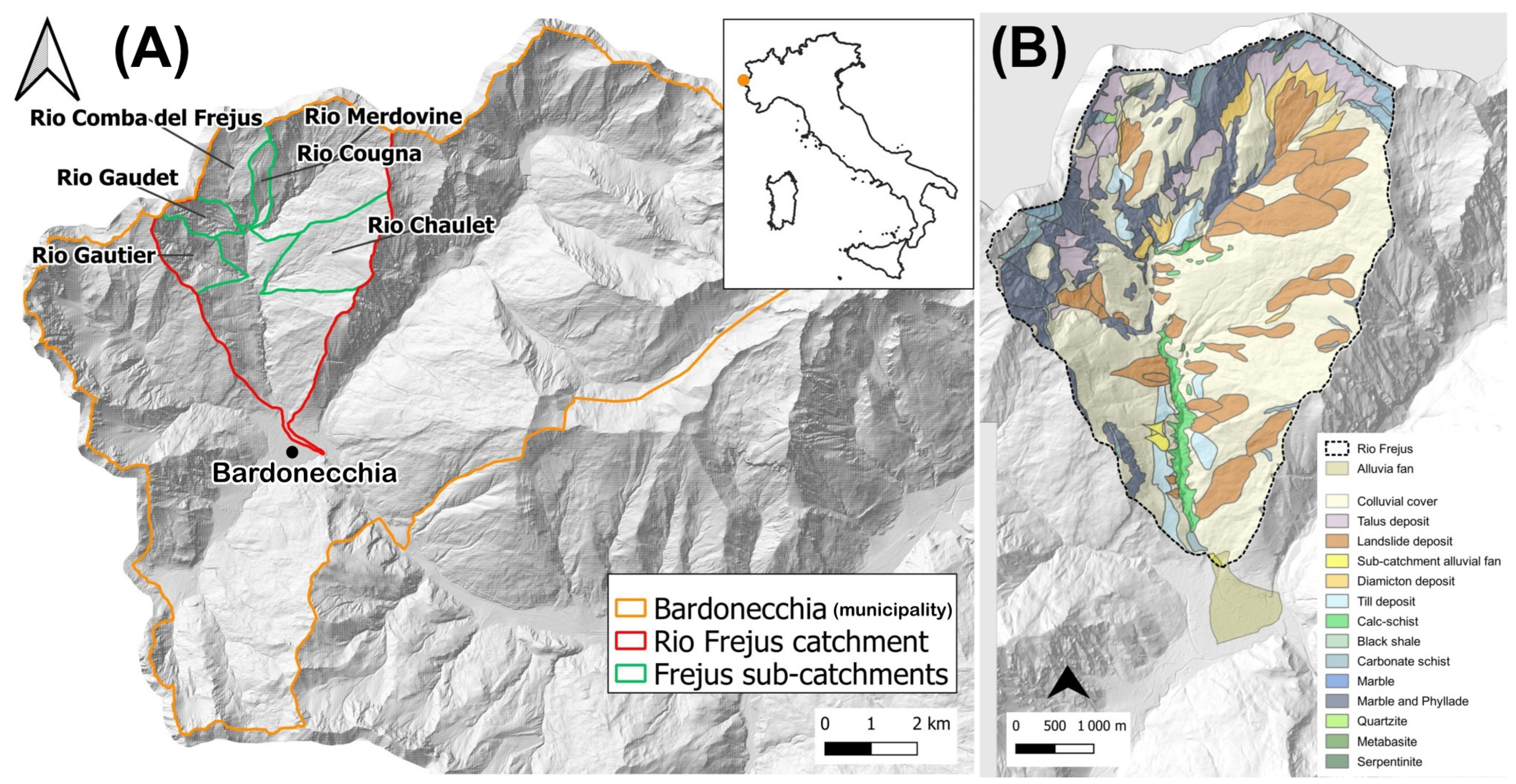
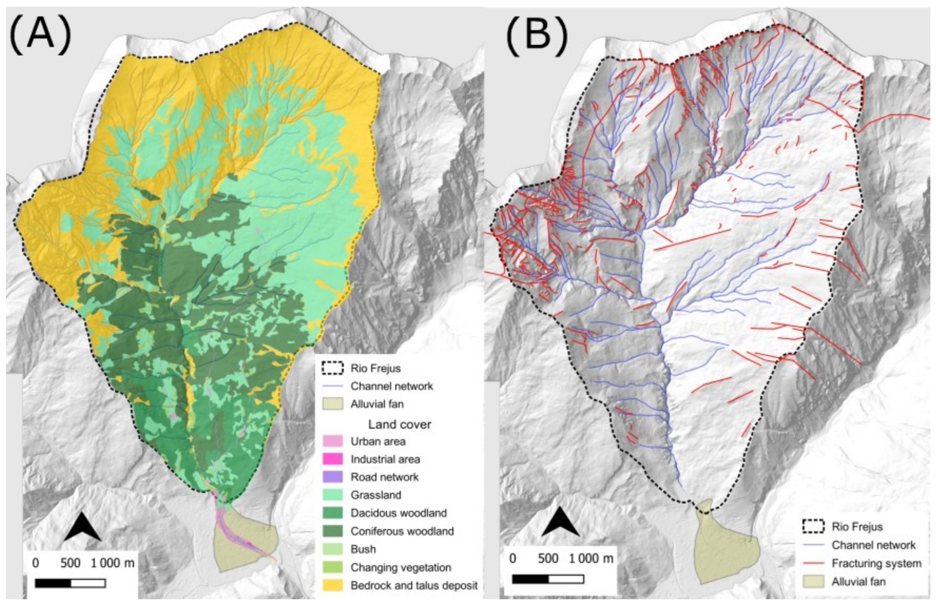
The Rio Frejus Catchment and Historical Series of Debris Flow Events

The Rio Frejus catchment (

Table 1. Main features of the Rio Frejus catchment.

Catchment Parameter	Value
Catchment area [km2]	22.32
Main incised channel length (from catchment head to alluvial fan toe) [km]	9.42
Average catchment slope [°]	28.1
Max elevation (at watershed) [m asl]	3.14
Min elevation (at alluvial fan toe) [m asl]	1.25
Average elevation [m asl]	2.19
Alluvial fan area [km2]	0.43
Fan/catchment area ratio [%]	1.93
Bedrock outcropping area [km2]	5.27
Bedrock outcropping percentage [%]	23.63
Landslide deposits area [km2]	8.56
Landslide deposits percentage [%]	38.36
Surficial deposits and eluvial–colluvial cover area [km2]	8.48
Surficial deposits and eluvial–colluvial cover percentage [%]	38.00

) is located in the municipality of Bardonecchia (Susa Valley, Western Italian Alps) in the province of Turin. The catchment, elongated north–south, has an area of about 22 km² and is subdivided into five sub-catchments, which correspond to the tributary channels of the main incised channel of the Rio Frejus (Figure 1A).

Given the geological and geomorphological characteristics of the catchment, it is affected almost annually by debris flow events, mainly of modest magnitude, during the summer storms (

Table 2. Historical debris flows have affected the Rio Frejus catchment since the 20th century, including the high-magnitude debris flow events of 6 August 2004, 7 August 2009 and 13 August 2023.

Sub-Catchment	Date	Time	Flow Type Observed at the Alluvial Fan
-	July 1914	-	-
-	September 1920	-	-
-	3 August 1934	-	mud–debris flow
-	12 June 1947	-	-
-	4 September 1948	-	-
Merdovine	2 May 1949	-	mud–debris flow
Merdovine	26 May 1951	-	mud–debris flow
-	21 June 1954	-	mud–debris flow
-	21 August 1954	-	mud–debris flow
-	8 June 1955	-	mud–debris flow
-	13 June 1957	-	-
-	18 October 1966	-	-
-	3 November 1968	-	mud–debris flow
Gautier	7 August 1997	4:15–4:30 p.m.	mud–debris flow
Gautier	21 June 2002	-	mud–debris flow
Gautier	6 August 2004	8:00 p.m.	debris flow
Gautier	25 July 2006	8:30 p.m.	mud–debris flow
Gautier, Merdovine and Gaudet	August 2006	-	mud–debris flow
Merdovine	7 August 2009	7:00 p.m.	debris flow
Gautier	16 July 2013	7:45 p.m.	mud–debris flow
-	17 July 2013	7:45 p.m.	mud–debris flow
-	9 August 2015	-	mud–debris flow
-	8 August 2017	7:30 p.m.	mud–debris flow
Merdovine	13 August 2023	9:00 p.m.	debris flow
Merdovine	30 July 2024	8:30–9:00 p.m.	mud–debris flow

), which originate especially from the Merdovine and Gautier sub-catchments.

Through field observations, the change in the flows along the channel network was identified, passing from a mature debris flow in the upper parts of the catchment to a mud–debris flow or hyperconcentrated flow in the alluvial fan area. This evolution is linked to the morphometry and lithological characteristics of the catchment.

The average annual rainfall in the upper Susa Valley is moderate to low, with a value of about 770 mm/yr, with more frequent and intense rainfall events between June and September.

The catchment is characterized by geological settings with high structural complexity, typical of the Western Alps. The ‘Lago Nero’ represents the main tectonostratigraphic unit of the outcropping bedrock [20]. This unit is primarily formed by carbonate schists rich in phyllosilicates with poor geomechanical characteristics that promote a continuous production of loose material, along with subordinate serpentinites and metabasites (Figure 1B) characterized by stronger geomechanical properties.

Where there are litho-structural conditions and slopes predisposing to gravitational instability, these rock masses assume a degree of gradually increasing loosening until complete disarticulation. These characteristics of the bedrock generate particularly favorable conditions for debris production, representing the main source area for the initiation of debris flow phenomena, as described by [19].

The surficial deposits can be distinguished into eluvial–colluvial, talus, glacial (till), landslide, alluvial fans and debris flow/hyperconcentrated flow (near the channel network) deposits. The debris accumulations are deeply engraved by numerous gullies and represent important sources of easily erodible material. The morphology of the catchment is complex and articulated due to the overlapping of different processes (glacial, erosive action of watercourses, slope processes).

2. Materials and Methods

2.1. Catchment Characterization: From Geological–Geomorphological Analyses to Debris Flow Susceptibility Assessment

Effective catchment characterization is crucial to identifying the initiation areas for implementing appropriate monitoring systems and strategies. This process helps identify the initiation areas and facilitate the adoption of suitable monitoring strategies.

A two-step approach was adopted in this study. First, the catchment was classified using the Clay Weathering Index (CWI) and the bedrock outcropping percentage threshold, as proposed by [19,21,22]. This approach assesses the lithological features of the bedrock, which produces mobilizable material influencing the debris flow behavior, taking into account the actual connection between the sediment source areas and the channel network. Second, susceptibility mapping was performed using a modified version of the Rock Engineering System (RES) method to determine the debris flow propensity index (DfPI) [23,24]. This step focused on identifying the most active initiation areas based on the geological and geomorphological characteristics of the catchment identified in the first step.

2.1.1. Lithological Catchment Classification

Small Alpine catchments (area ≤ 50 km²) are subject to different flow types, influenced by specific characteristics that also govern flow behavior in terms of sediment concentration, rheology, occurrence frequency, seasonality and triggering causes. Tiranti et al. [16,21] proposed a novel classification method based on the Clay Weathering Index (CWI). This method describes debris flow behavior by assessing the dominant lithology of the catchment bedrock and its propensity to produce varying amounts of clay-size sediments.

The CWI identifies three main classes:

• Excellent Clay Maker (ECM): catchment bedrock mainly formed by thin-foliated metamorphic rocks, producing high quantity of clay grain-size sediments.
• Good Clay Maker (GCM): catchment bedrock mainly formed by massive carbonate rocks, producing moderate quantity of clayey silt grain-size sediments.
• Bad Clay Maker (BCM): catchment bedrock mainly formed by massive crystalline rocks, producing negligible quantity of fine sediment.

The amount of clay in the fine sediment influences the flow rheology: (i) >5% for cohesive debris flows (viscoplastic behavior); (ii) <5% for non-cohesive debris flows (frictional–collisional behavior). The CWI also describes the characteristics of alluvial fans:

• ECM alluvial fans have a small size compared with the size of the feeding catchment (normally, the fan area is about 5% of the catchment area), with an irregular shape and low grain-size differentiation along the longitudinal axis of the fan (from apex to toe). The most frequent debris flow deposits are represented by clayey matrix-rich asymmetric levees in the cross-section with steep sides.
• GCM alluvial fans have a large size compared with the size of the feeding catchment (normally, the alluvial fan area is about 20% of the catchment area), with a regular flat-fan shape and low grain-size differentiation along the longitudinal axis of the fan (from apex to toe). The most frequent debris flow deposits are represented by clayey silt matrix-rich symmetric levees with a flat shape in the cross-section.
• BCM alluvial fans have a moderate size compared with the size of the feeding catchment (normally, the alluvial fan area is about 10% of the catchment area), with a regular lobate shape and high grain-size differentiation along the longitudinal axis of the fan (boulders in the apex area and silty sands at the toe, through abrupt transitions). The most frequent debris flow deposits are represented by matrix-free (or scarce silty sand matrix) levee-like boulder trains.

Further studies [22], updated in [19], also emphasize the role of the catchments’ bedrock outcropping percentage in determining the predominant flow process likely to occur. These processes are also related to the features of the coarse sediment fraction in loose material. This methodology identifies the following outcropping bedrock percentage thresholds for different flow types:

• Outcropping bedrock < 20% generates water flows.
• Outcropping bedrock ≥ 20%–≤54% generates hyperconcentrated flows.
• Outcropping bedrock ≥ 55% generates debris flows.

These methodologies were applied to classify the Rio Frejus catchment to identify the debris flow predisposing factors, the main rheology of the flow processes and the debris flows’ depositional style (including sedimentological characteristics and depositional patterns). Additionally, they helped define the alluvial fan architecture and establish the rainfall triggering threshold values for debris flow initiation via the correlation of observed rainfall and historical debris flow events [16,19,21].

2.1.2. Debris Flow Propensity Index Assessment

Lithological classification is also valuable for further catchment characterization, particularly in identifying the most susceptible areas within the catchment. This susceptibility mapping is crucial for designing a monitoring system that ensures these critical zones are effectively observed, especially in mountainous catchments subdivided into multiple sub-catchments, such as the Rio Frejus catchment.

The analysis was conducted using a modified version of the DfPI approach proposed by Bonetto et al. and Vianello et al. [23,24]. The methodology is based on the RES method proposed by Hudson [25], an expert semi-quantitative method designed to describe and evaluate the relationships and interactions among the factors influencing, in this case, a debris flow phenomenon.

The DfPI quantifies the susceptibility to debris flow generation based on a set of primary predisposing factors. The score ranges from 0 (low susceptibility) to 100 (extreme susceptibility) and is calculated using Equation (1):

$$DfPI={\sum }_{\hspace{0.17em}i=0}^{\hspace{0.17em}n}\left(a_i\cdot P_{ik}\right)$$

(1)

where a_i is the weighting coefficient for the i-th parameter, and P_ik is a specific value between 0 (most stable condition) and 4 (most favorable condition) assigned to each class of the identified predisposing factors.

The weighting coefficient can be calculated using Equation (2) as

$$a_i={\displaystyle \frac{1}{\max \left(I_{ijth}\right)}}\cdot {\displaystyle \frac{C+E}{\sum C+\sum E}}\cdot 100$$

(2)

where I_ijth, C and E are evaluated after generating the interaction matrix. In this matrix, the main predisposing factors are placed along the main diagonal, while the off-diagonal terms represent interactions between the i-th parameter and the (i + 1)-th parameter.

In this matrix, C represents the sum of values in each row (Cause—C), indicating the influence of parameter Pi on the system, and E is the sum of values in each column (Effect—E), representing the influence of the system on parameter Pi.

Compared to the previous version of DfPI [24], where bedrock lithology, surficial deposits, slope, channel network, curvature, land use, lineament density and landslide activity were encoded into two matrices, A and B, for outcropping lithologies and surficial deposits, respectively, this study modified and updated the interaction matrices. Specifically, the channel network and curvature—two key geomorphological parameters—were replaced with the connectivity index (CI), as described in the following sub-section. All of these parameters and their corresponding indices were obtained directly or with minimal analysis from freely available databases:

• Outcropping lithologies and surficial deposits were derived from the ‘Foglio 153—Bardonecchia’ of the Geological Map of Italy at the scale of 1:50,000 [26].
• The slope and connectivity index were derived from the 5 × 5 m regional digital elevation model (DEM). Slope was calculated using the QGIS 3.4 software’s slope calculation tool. The procedure for deriving the CI is described in Section 2.1.3.
• Land use was obtained from the metadata of the Land Cover Piemonte 2021 project (https://geoportale.igr.piemonte.it/cms/progetti/land-cover-piemonte, accessed on 15 November 2024).
• Landslide distribution and activity were derived by merging the information from the Italian Landslide Inventory (IFFI, https://www.progettoiffi.isprambiente.it/, accessed on 15 November 2024) and the Landslide Information System of Piedmont region (SIFraP, https://www.arpa.piemonte.it/dato/sistema-informativo-frane-piemonte-sifrap, accessed on 15 November 2024).

Furthermore, to incorporate the lithological classification previously described, as well as the characteristics of the non-flow-like landslides that affected the study area, the P_ik values for these parameters were modified accordingly.

As stated in [24], one of the main advantages of the RES approach is its integration with GIS-based software. Similarly, in this study, the 5 × 5 m regional DEM was used as a basemap for performing the susceptibility analysis, resulting in a DfPI index for each cell of the DEM.

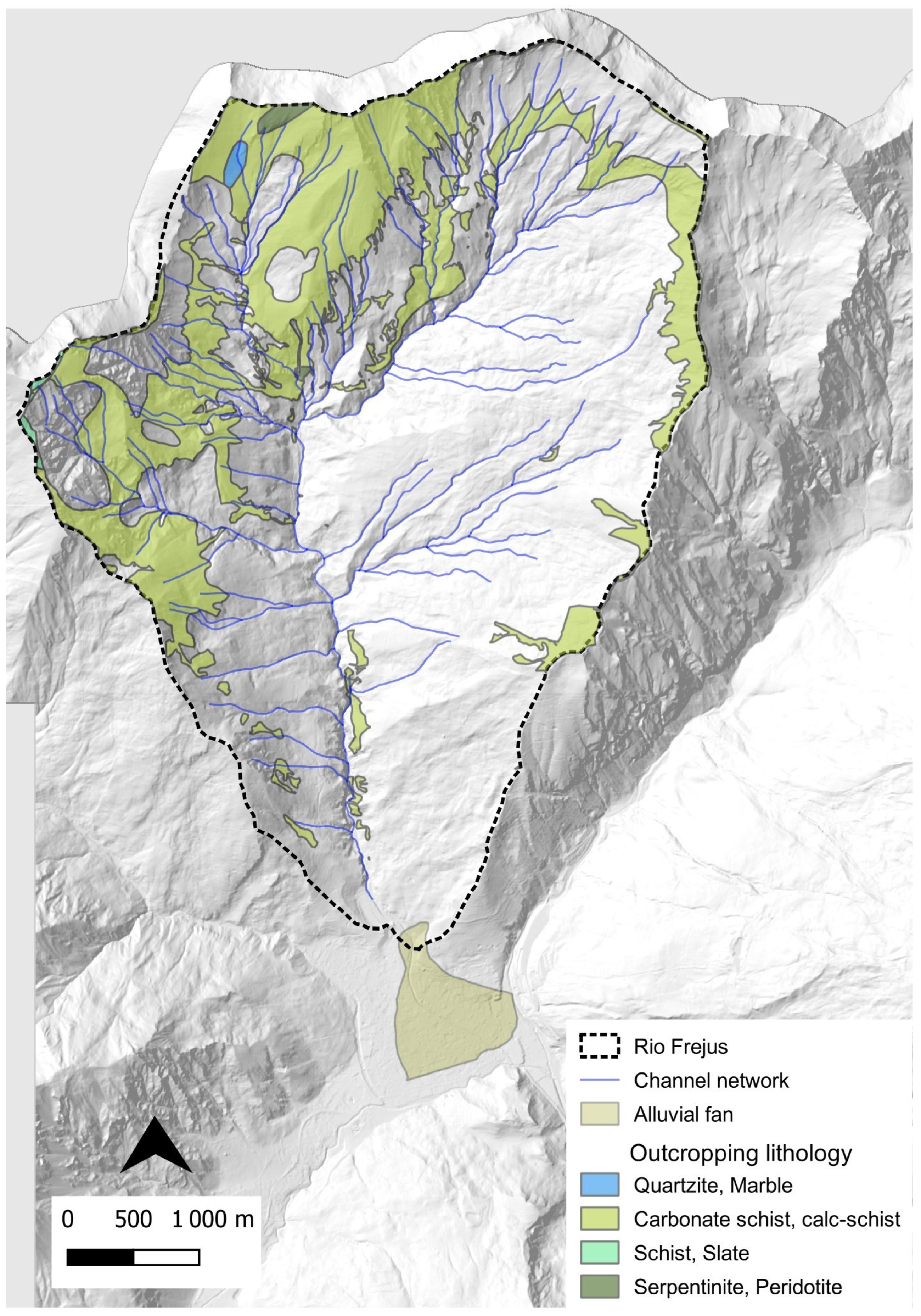
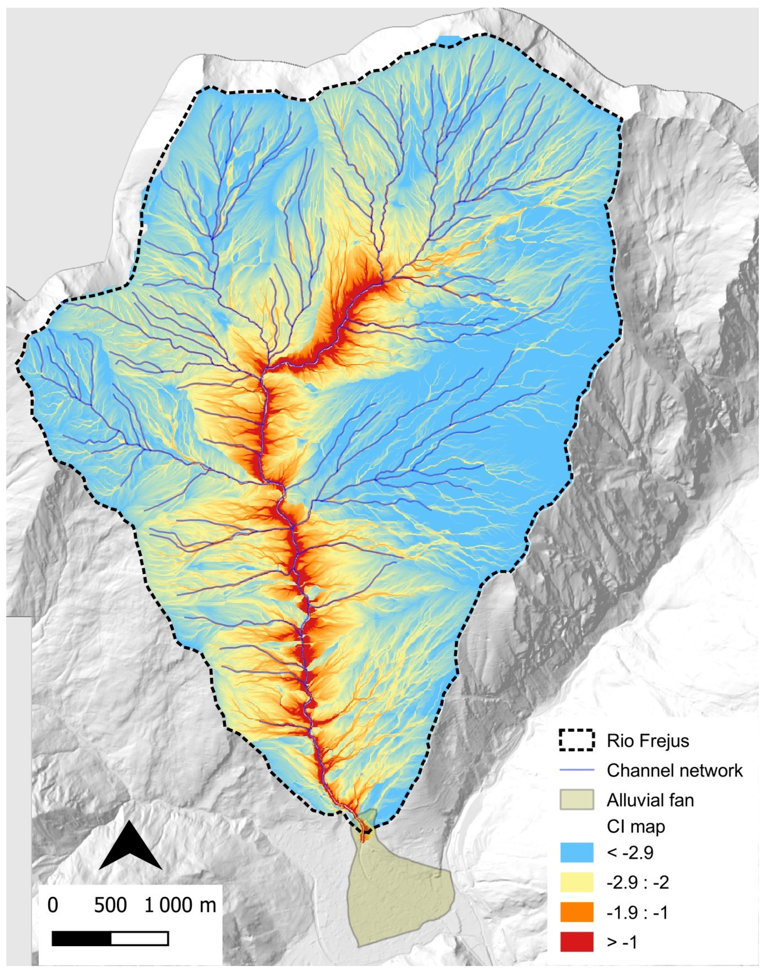
2.1.3. Connectivity Index

Sediment connectivity analysis was performed to characterize and identify the sediment source areas, focusing on their connection to the main drainage system.

The sediment connectivity index (CI) is a topography-based index, originally developed by Borselli et al. [27] and adapted to mountain environments by Cavalli et al. [28]. Using a high-resolution DEM, a CI map of the catchment can be generated by calculating the logarithm of the ratio between the upslope (D_up) and downslope (D_dn) components for each cell, as described in Equation (3):

$$CI=\log \left({\displaystyle \frac{D_{up}}{D_{dn}}}\right)$$

(3)

The upslope component expresses the potential for downward routing of sediment, while the downslope component represents the sediment flux path length to the nearest target sink (Equation (4)):

$$D_{up}=W\cdot S\cdot A\hspace{0.17em}\hspace{0.17em}\hspace{0.17em}\hspace{0.17em}\hspace{0.17em}\hspace{0.17em}{D}_{dn}=\sum {\displaystyle \frac{d_i}{W_i{S}_i}}$$

(4)

Both components incorporate a weighting factor that accounts for flow impedance due to topographic influence on sediment connectivity. Borselli et al. [27] initially evaluated this factor using vegetation (land cover) as an indicator, while Cavalli et al. [28] proposed using surface roughness to better capture the effects of morphology and topography on runoff processes (Equation (5)):

$$W=1-{\displaystyle \frac{RI}{R{I}_{max}}}$$

(5)

The CI map was calculated using the SedInConnect tool [29]. The necessary input is the DEM of the area, previously modified with QGIS 3.4 to remove small local depressions that could interfere with the connectivity analysis. In addition, the size of the DEM cells (5 m resolution), the targeted stream tract and the use of roughness for the weighting factor calculation had to be indicated.

The result was classified into four categories (low, medium-low, medium-high and high) using the natural breaks classification algorithm.

The CI method was applied to the Rio Frejus catchment to identify the sediment source areas that are effective in supplying debris flow events, which can reach the alluvial fan area, as previously proposed [18].

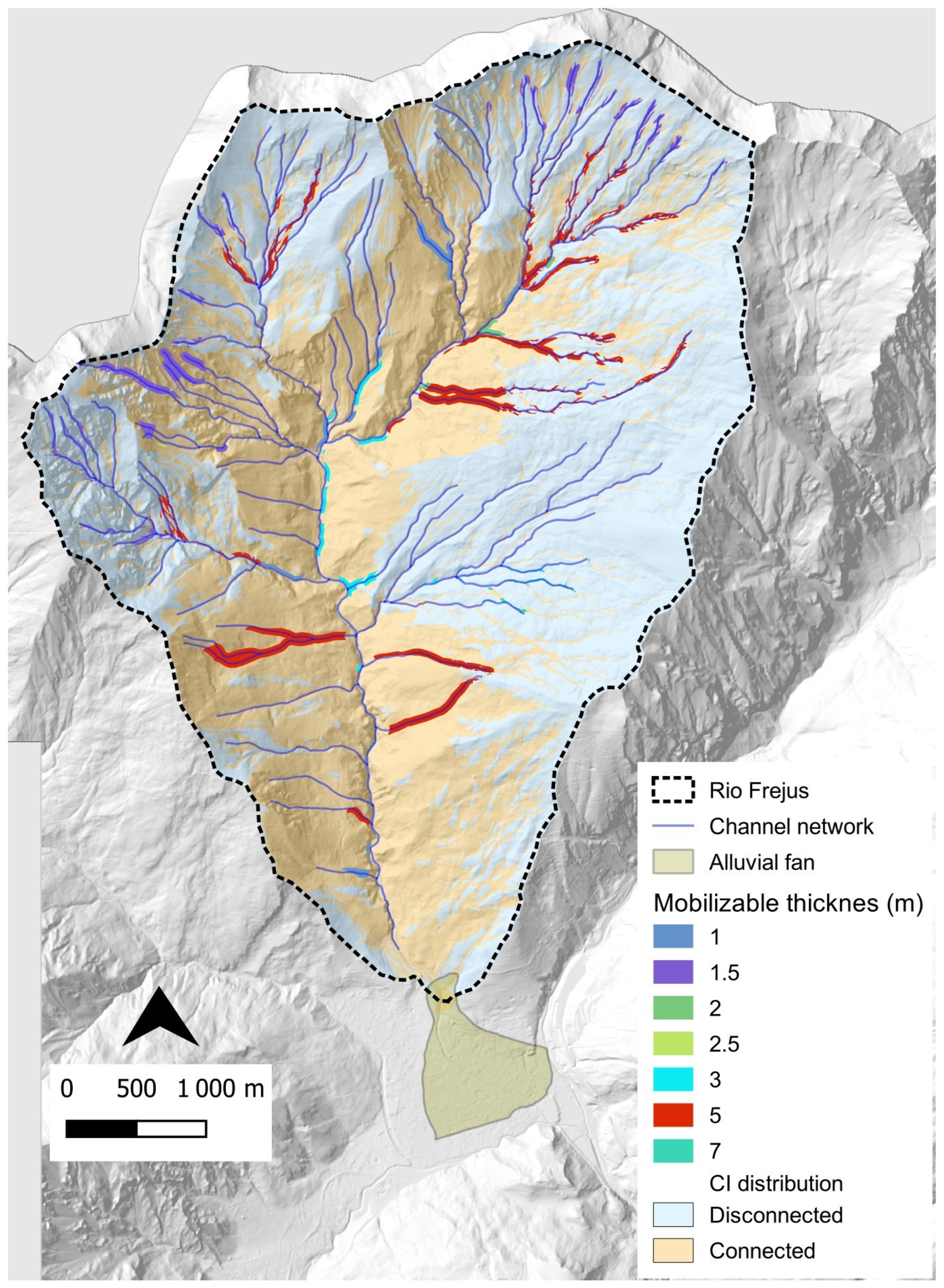
2.1.4. Sediment Source Area Estimation

Commonly, debris flow phenomena occur where the channel network intersects the main surficial deposits. For this reason, sediment source areas were estimated considering the intersection between landslide/talus deposits and the channel network.

Landslide deposits can be generated from different types of movement, such as rock falls, rotational slides, large shallow landslides and earth flows, each presenting different characteristics in terms of size, activity and sedimentological features. Sediment sources can be located both at the heads of the catchment and along the slopes. Additionally, an important sediment source is represented by stream deposits along the channels, resulting from past debris flow events.

In this research, the most probable amount of sediment capable of contributing to a debris flow was determined by considering a 50 m buffer around the channel axes intersecting the main surficial deposits within the catchment, according to [18]. These deposits were identified and described through field surveys, aerial photo interpretation and thematic layers from public repositories (Geoportale Regione Piemonte, https://www.geoportale.piemonte.it, accessed on 15 November 2024; Geoportale of ARPA Piemonte, https://geoportale.arpa.piemonte.it, accessed on 15 November 2024).

2.2. Debris Flow Monitoring

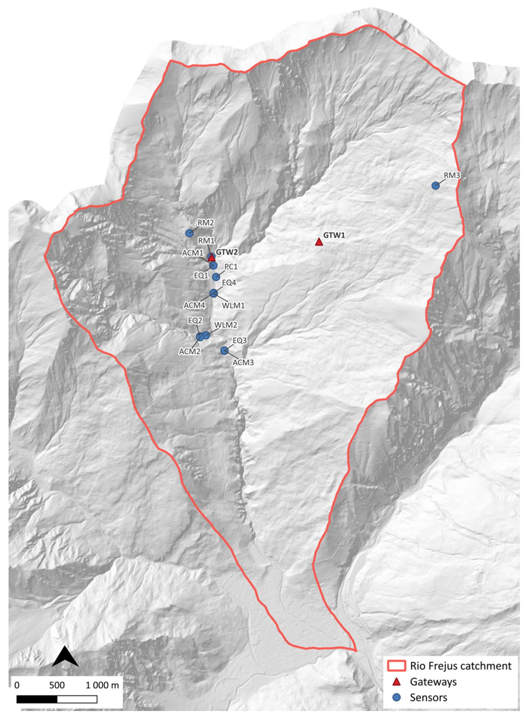
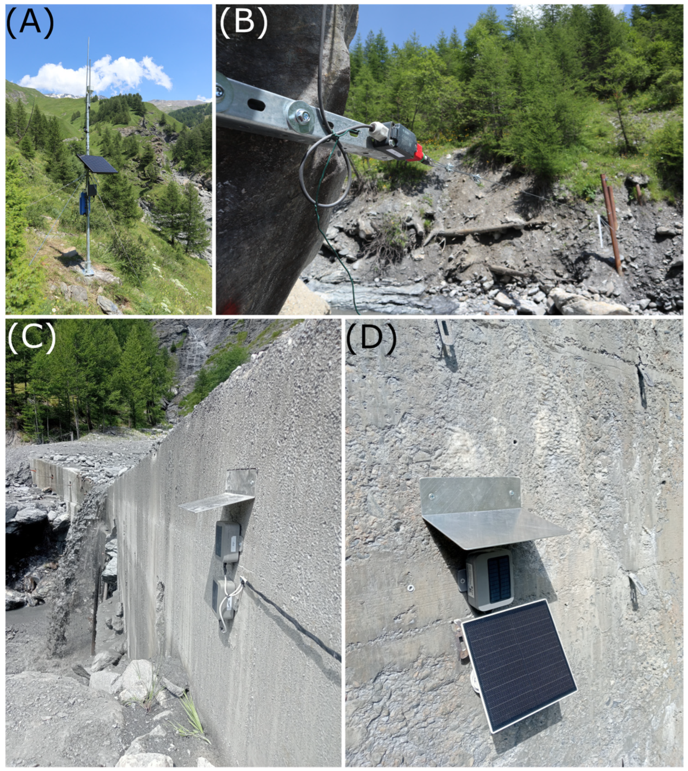
2.2.1. Monitoring System

The results of the analyses described in the previous section, coupled with the historical dataset of events, assist in designing a monitoring system for this area.

A monitoring system was developed to analyze both the triggering factors and propagation behavior of debris flows within the Rio Frejus catchment. This stage can be useful for future development of an early warning system to support decision making by the authorities. Most of the effort was directed toward monitoring the upper part of the catchment, where most of the triggering areas are located. However, the propagation of the phenomenon was also monitored through installation of various multi-sensor stations on the hydraulic protection works along the Rio Frejus channel network.

Table 3. Monitoring sensors installed.

Sensor	Number	Sampling Frequency	Unit of Measure	Sensitivity	Range
Rain gauge (RM)	3	30 s	mm	0.25 mm	0-Inf
Accelerometer (ACM)	4	30 s	m/s2	0.01 m/s2	±2 g
Seismic sensor (EQ)	4	30 s	m/s2	0.01 m/s2	±2 g
Water level meter (WLM)	2	30 s	mm	1 mm	0.5–10 m
Pull-cord (PC)	1	30 s	/	/	0–1

lists the types of sensors installed within the Rio Frejus catchment and their main characteristics. From the head to the bottom of the catchment, the sensor network includes three rain gauges (RM in Figure 2) installed at an altitude of 1764 m asl (RM1, at the closing of the Rio Comba Frejus sub-catchment), 2055 m asl (RM3, monitoring Rio Merdovine sub-catchment) and 2648 m asl (RM2, monitoring Rio Gaudet sub-catchment). Additional sensors were installed downstream to monitor the evolution of the flow. Specifically, they were organized into five monitoring stations (Figure 3), distributed as shown in Figure 2:

• Station 1 (1731 m asl): monitoring the Rio Frejus main channel (at the confluence with Rio Merdovine, Rio Gaudet and Rio Comba Frejus) and equipped with a seismic sensor (EQ1) and accelerometer (ACM1).
• Station 2 (1688 m asl): monitoring the Rio Frejus main channel (downstream of the confluence with Rio Merdovine, Rio Gaudet and Rio Comba Frejus) and equipped with a seismic sensor (EQ4), accelerometer (ACM4) and water level meter (WLM1).
• Station 3 (1711 m asl): monitoring the Rio Frejus main channel (downstream of the confluence with Rio Merdovine, Rio Gaudet and Rio Comba Frejus) and equipped with a pull-cord (PC1).
• Station 4 (1680 m asl): monitoring the Rio Gautier sub-catchment (close to the confluence with the Rio Frejus main channel) and equipped with a seismic sensor (EQ2), accelerometer (ACM2) and water level meter (WLM2).
• Station 5 (1613 m asl): monitoring the Rio Frejus main channel (downstream of the confluence with Rio Gautier) and equipped with a seismic sensor (EQ3) and accelerometer (ACM3).

To provide a clear description of the debris flow propagation, the selected sensors enable real-time data acquisition regarding the flow height within the stream, the intensity of vibrations induced in the ground and on structures and the dissipation of energy from the phenomenon.

The implementation of two gateways (GTW1 and GTW2) ensures seamless data transmission and real-time communication between the remote sensors and the remote data collecting center.

The wireless communication technology used by the sensors employs the LoRa WAN protocol, which offers the advantages of covering large areas with low power consumption. The sensors were connected via two gateways (GTW1 at 2155 m asl and GTW2 at 1760 m asl in Figure 2), enabling data transmission with central management control. Since the gateways need to be linked to the sensors and require a direct internet connection, a visibility analysis was performed to determine their optimal locations. The sensors’ locations were chosen to cover most of the catchment area, with a focus on accessible sections where protection structures are present, allowing for analysis of their response to the flow passage.

All sensors and gateways are powered by batteries, which are recharged via external solar panels. During installation, the instruments were permanently set up in a safe position along the section and secured with metal shields to protect them during high-magnitude flow events.

Access to real-time monitoring is ensured through communication between the gateways and an online dashboard, which samples the signal every 30 s and displays the values of the variables, as well as other data related to signal quality and battery status. The monitoring system is also visualized spatially through a WebGIS integrated with a data management dashboard, where the position and attributes of each component are highlighted, and the corresponding measurements are linked. The WebGIS allows users to view the details of each sensor, and by selecting a measurement point, the corresponding data time series is displayed.

2.2.2. Unmanned Aerial Vehicle (UAV) Photogrammetry

The findings from Section 2.1 allow the identification of the primary triggering areas within the catchment. However, no information about the potential mobilizable volume or the mobilizable material recharge rate can be obtained from the methods described previously. Similarly, the installed sensors of the monitoring system can only provide information on the rate of entrainment or deposition in localized sectors of the catchment, but they do not offer insight into the available loose material potentially mobilizable at the head of the catchment. Consequently, a preliminary attempt to evaluate the potential event magnitude at the source area was made by employing a remote aircraft. Based on accessibility and the feasibility of safely operating a remote aircraft at these sites, a 22-hectare area within the Rio Merdovine sub-catchment was selected for further analysis. The goal of this survey campaign was to collect data for a change detection analysis using the digital elevation models of difference (DoD) approach. This method utilizes a pair of digital elevation models representing the same area at two different acquisition times to compute the ground difference resulting from a specific event.

The equipment used for the survey included a DJI Mavic 3 unmanned aerial vehicle (UAV) (

Table 4. UAV DJI Mavic 3 technical data.

UAV DJI Mavic 3
RGB camera	CMOS 4/3″
Sensor length [mm]	13
Sensor width [mm]	17.3
Sensor resolution [MP]	20
Image dimension [px]	5280 × 3956
Focal length [mm]	24

), a Geomax Zenith 60 GNSS antenna with RTK correction and water-based spray paint for marking the points used to georeference the model.

The planning of the survey operation began with the evaluation of flying permissions for the area. According to official maps provided by the Civil Aviation Authority (National Agency ENAC), the area has no restrictions below 120 m from the ground. The planning also took into account other factors, such as the area of interest, which needs to be covered uniformly. Additionally, the flying altitude was considered, as it is directly related to the ground sampling distance (GSD). The positioning of ground control points (GCPs) is another key consideration, as the RTK correction used by the GNSS antenna requires access to an online network, and the points must be distributed across the entire area. After identifying and measuring the coordinates of the GCPs using the GNSS antenna, the flight was operated manually in the first survey and automatically in the second one, maintaining a constant altitude to ensure a consistent GSD.

The acquired data were processed using the structure from motion (SfM) algorithm, a photogrammetric technique employed to reconstruct 3D structures from a series of 2D images. By identifying common points across multiple photographs, SfM algorithms estimate both the camera positions and the 3D coordinates of the scene. This process enables the creation of accurate 3D models and digital elevation models (DEMs) from aerial imagery. The workflow involved selecting high-quality images from the dataset, performing image alignment and generating a point cloud, which was then georeferenced using the coordinates of the GCPs. These coordinates were imported into the software to ensure precise georeferencing of the model. Subsequently, a dense point cloud was processed, and a mesh was created from which the DEM was derived.

Two acquisition campaigns were conducted in the selected area (

Table 5. Survey conducted.

Date	Images	Designed GSD	Obtained GSD	Flight Altitude
Survey 1: 30 July 2024	4825	3.2 cm	5 cm	Manual
Survey 2: 20 August 2024	3618	4.75 cm	5 cm	75 m

): the first, serving as a reference for future surveys, was carried out concurrently with the installation of the monitoring system, and the second, conducted three weeks later, aimed to detect any potential changes in deposits within the source area. Between the two surveys, two small debris flow events were recorded.

The same procedure previously described was applied to both surveys. For the DoD results, the DEMs obtained from the two acquisitions were properly sampled and aligned before being subtracted.

3. Results

3.1. The Rio Frejus’ Debris Flow Susceptibility of Initiation Areas

The approaches presented in Section 2.1 allowed the identification of sectors most susceptible to debris flows within the Rio Frejus catchment. The results of the susceptibility assessment and flow process characterization were used to guide the design and installation of the monitoring system described in Section 2.2. The implementation of this system allowed us to record a debris flow event in the summer of 2024, and the collected data were used to validate and confirm the results obtained from preliminary investigations to characterize the catchment.

The Rio Frejus catchment was classified as ECM, applying the CWI approach, because the dominant lithology forming the catchment’s bedrock consists of carbonate shists and calc-schists, constituting 96.32% of the rock outcrops, as illustrated in Figure 4.

According to the CWI classification, the debris flows in the Rio Frejus are characterized by viscoplastic rheology due to the high percentage of clay in fine sediments (>5%) produced by the outcropping rocks as loose material.

Moreover, the poor geomechanical properties of the dominant rocks forming the catchment promote a large production of coarse loose material (Figure 5), mainly derived from frequent small rockfalls. The coarse fraction of loose material comprises.

• Rare boulders between 1 and 2 m³, showing sphericity ranging from prismoidal to sub-prismoidal, and occasionally spherical, with roundness from angular to very angular.
• Common blocks sized 0.50–0.70 m³, exhibiting sphericity from prismoidal to sub-discoidal and roundness from angular to very angular.
• Abundant cobbles and pebbles, with sphericity from prismoidal to discoidal and roundness from angular to very angular.
• Very abundant gravels characterized by sphericity from prismoidal to discoidal and a very angular roundness.

High clay content favors the initiation of cohesive debris flows, which are characterized by high viscosity, conferring to the flow a viscoplastic rheology [17] and resulting in moderate-to-low velocity. High viscosity causes most of the material transported by the debris flow to settle relatively close to the trigger area. As the debris flow propagates, it becomes progressively diminished in the solid component, eventually reaching the fan area as a diluted solid–liquid mixture with characteristics of a hyperconcentrated flow or mud flow. Commonly, more than 30% of sediments are deposited in the medium-high parts of the catchment.

As a result, the alluvial fan of Rio Frejus is relatively small compared to the feeding catchment, with an alluvial-fan-to-catchment-area ratio of 1.93%. The deposition of debris flows in the upper part of the catchment determines the conditions of starved aggradation of the alluvial fan, and a low–moderate average magnitude of the events, until large quantities of sediment progressively accumulated in the head areas of the catchment are mobilized by high-intensity rainstorm events. Such events occurred on 6 August 2004 and 13 August 2023, generating two high-magnitude debris flows that reached the alluvial fan area.

In the Rio Frejus catchment, as an ECM catchment, debris flows are commonly triggered by rainstorms of low–moderate intensity, with a minimum triggering threshold of 20 mm/h (intensity of a 5-year return period in the Susa Valley) [21]. This threshold is confirmed by the frequency and seasonality of debris flow events (see Table 2). In fact, the higher occurrence of debris flow events along the Rio Frejus catchment takes place during summer, when rainstorms are more frequent. Moreover, the high recurrence of flow phenomena (close to one per year) is testament to the high production of loose material by the outcropping rocks, ensuring a constant sediment supply that can be mobilized by debris flows, even in the face of low-intensity rainstorms [19].

Regarding the bedrock outcropping percentage thresholds that determine the type of flow most likely to reach the alluvial fan area, as described in Section 2.1.1, the Rio Frejus catchment has an outcropping percentage of 23.63%. This value overcomes the threshold of 20%, indicating a high probability that a hyperconcentrated flow will reach the alluvial fan area.

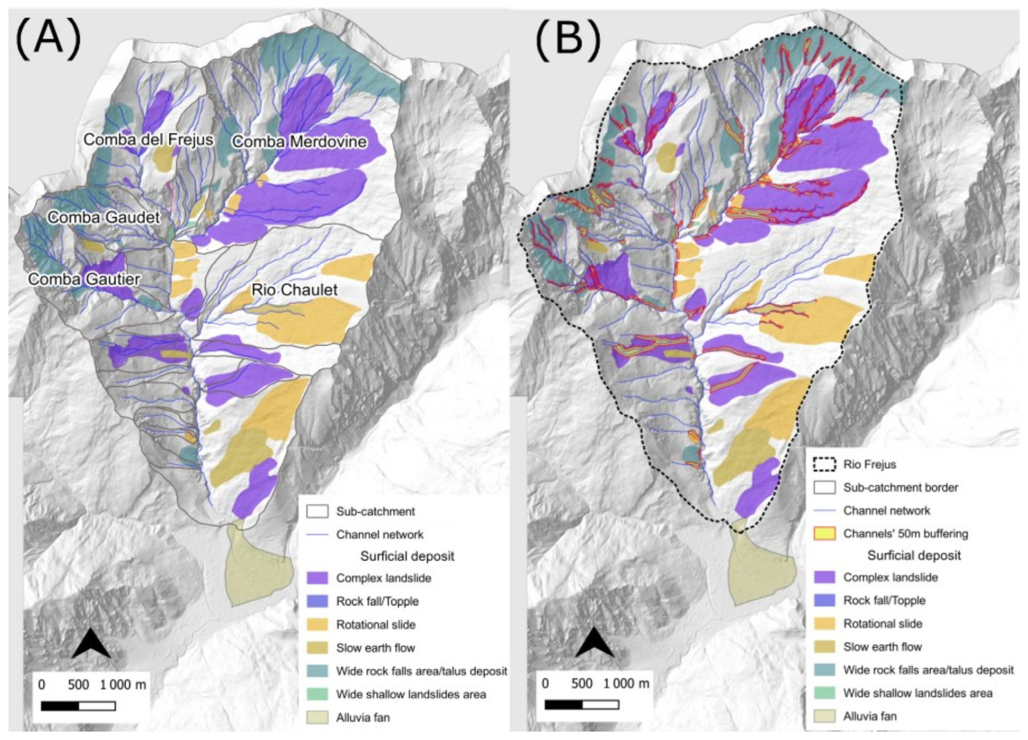
3.2. Actual Sediment Source Areas

To estimate the actual sediment source areas that can contribute to debris flow feeding, the identified surficial deposits were mapped and classified through field surveys and aerial photo analysis (Figure 6A). These deposits were related to the channel network, considering a 50 m buffer as the effective area of interaction between deposits and channels (Figure 6B).

In the second step, the connectivity index (CI) map was derived using the SedInConnect application [28]. The main channel was selected as the target.

Finally, the resulting raster was divided into four classes, following the natural breaks classification [18] (Figure 7).

Using an assessment of the sediment source area connectivity, it is possible to evaluate and select the areas connected to the main channel network. This excludes the portions of the catchment that are unable to transport material to the main incised channel.

The results of the connectivity index analysis were integrated with field observations to characterize the sediment source areas, including sedimentological characteristics of the deposits and their average thickness.

Obviously, the only representation of connectivity is not sufficient to provide an indication of susceptibility to the phenomenon, as it is also necessary to consider its intersection with the distribution of sediment source areas. According to [18], the most likely amount of sediment that can contribute to debris flow feeding is determined by selecting a 50 m buffer from the channel axes at the source areas (Figure 8).

Figure 8 shows that not the entire extent of sediment source areas (see Figure 6B) crossed by channels is capable of feeding debris flow phenomena. Instead, only portions of these areas, characterized by high connection in a restricted area near the channels, are relevant. This also considers the average thickness of the mobilizable material, which allows for a rough estimation of the likely initial debris flow magnitude. For this reason, the intersection between the source areas and the connectivity index map helps identify the most critical areas for monitoring. Furthermore, based on historical events, areas located in the lower portion of the catchment can be excluded, as debris flow typically originates from the catchment head.

3.3. Debris Flow Susceptibility Estimation

The identified debris flow predisposing factors—lithology and surficial deposits (Figure 1B), slope, connectivity (Figure 7), land use (Figure 9A), landslide deposit (Figure 1B) and fracturing systems (Figure 9B)—were processed using the methodologies described in Section 2.1.2 applied to the Rio Frejus catchment and classified according to their influence on debris flow initiation.

The data collected from public repositories and field surveys were cross-processed using a matrix approach.

In the analysis of debris flow susceptibility and estimation of DfPI, the distribution of surficial deposits and the outcropping lithology must be considered as independent parameters. The former is related to a potentially mobilizable volume, while the latter can create loose deposits depending on the mechanical characteristics of the rocks, as already highlighted in the previous analyses. Therefore, two interaction matrices were created to separately analyze the reciprocal interaction between bedrock lithology (Matrix A) or deposits (Matrix B) and the other parameters (

Table 6. Interaction Matrix A.

Matrix A—Lithology
a/a	1	2	3	4	5	C	C + E	ai
1	Lithology	2	2	1	1	6	10	3.57
2	0	Slope	4	3	0	7	17	6.07
3	0	3	Connectivity	2	1	6	18	6.43
4	1	2	2	Land use	0	5	12	4.29
5	3	3	4	1	Fracturing density	11	13	4.64
E	4	10	12	7	2		70	25

and

Table 7. Interaction Matrix B.

Matrix B—Deposits
a/a	1	2	3	4	5	C	C + E	ai
1	Deposits	2	2	2	2	8	19	4.85
2	4	Slope	4	3	3	14	23	5.87
3	3	3	Connectivity	2	3	11	21	5.36
4	1	2	2	Land use	1	6	16	4.08
5	3	2	2	3	Landslide activity	10	19	4.85
E	11	9	10	10	9		70	25

).

After coding the interactions of the main factors and calculating their weighted coefficients (Table 6 and Table 7), they were linearly correlated with the relevant thematic levels to produce a map of likely debris flow initiation areas (

Table 8. Classification and scores of predisposing factors considered in interaction matrices A and B for the application of RES.

Matrix A—Lithology			Matrix B—Deposits
Parameter	Class	Pj	Parameter	Class	Pj
Lithology	Quartzites	0	Deposits	No deposit	0
	Gneiss, quartz mica schist	1		Talus deposits	2
	Marble and dolostone	2		Glacial deposits	2
	Calc-schist and mica schist	4		Landslide deposits	3
	Gypsum and carbonate breccias	4		Eluvial–colluvial deposits	4
Slope	0–8°	0	Slope	0–8°	0
	9–15°	1		9–15°	1
	16–25°	3		16–25°	3
	26–35°	4		26–35°	4
	>35°	2		>35°	2
Connectivity	Low (≤−2.9)	1	Connectivity	Low (≤−2.9)	1
	Medium-low (−2.9: −2.3)	2		Medium-low (−2.9: −2.3)	2
	Medium-high (−2.3: −1.3)	3		Medium-high (−2.3: −1.3)	3
	High ≥ −1.3)	4		High (≥−1.3)	4
Land use	Villages, urban	0	Land use	Villages, urban	0
	High forests	1		High forests	1
	Low forests	2		Low forests	2
	Grassland	2		Grassland	2
	Rock and deposits	4		Rock and deposits	4
Fracturing density	Weak	0	Landslide activity	--	0
	Moderate	1		Nd	1
	Strong	2		Stabilized	2
	Very Strong	3		Quiescent	3
	Intense	4		Active	4

). This was performed using Equation (1) for calculating the DfPI, applying it to each cell of the 5 × 5 m grid generated within the catchment.

The classification of the raster map was carried out using a modified version of Brabb [30] susceptibility scale: Low (0–20), Medium (20–40), High (40–60), Very High (60–80) and Extreme (80–100) (Figure 10).

The resulting map confirms that the sub-catchments most susceptible to debris flow initiation are Rio Merdovine (northeast) and Rio Gautier (west), which should be the focus of any monitoring.

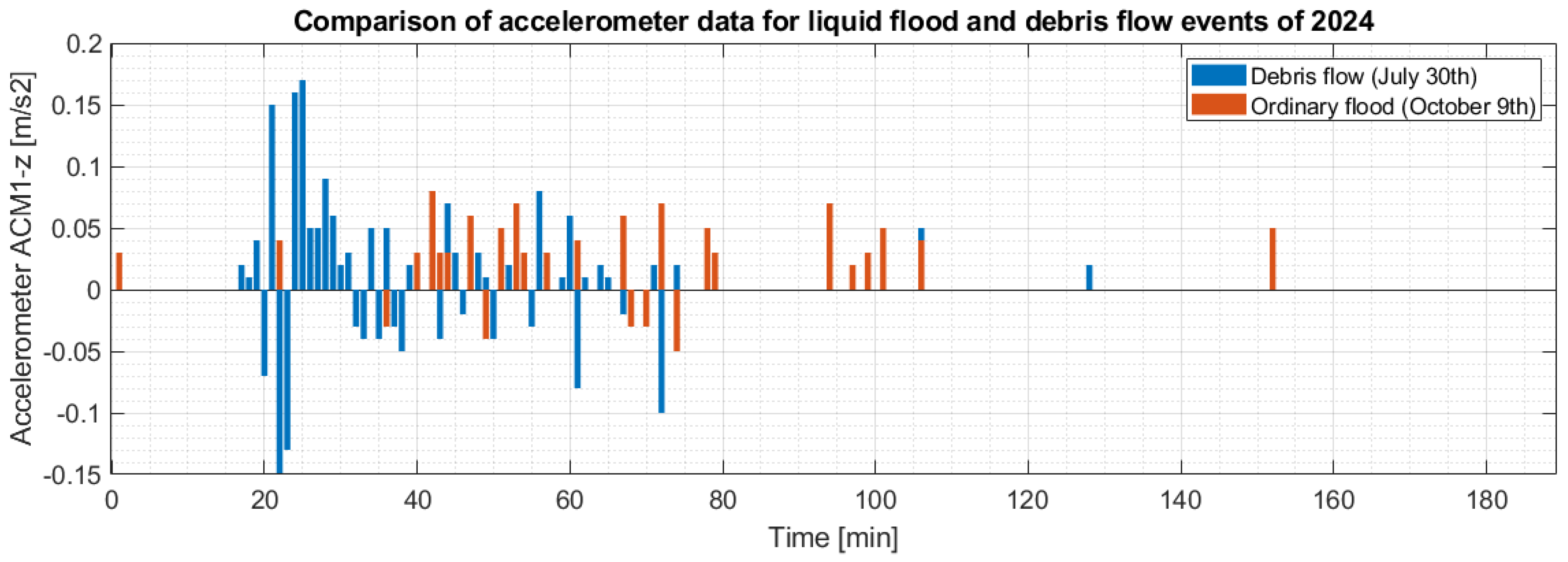
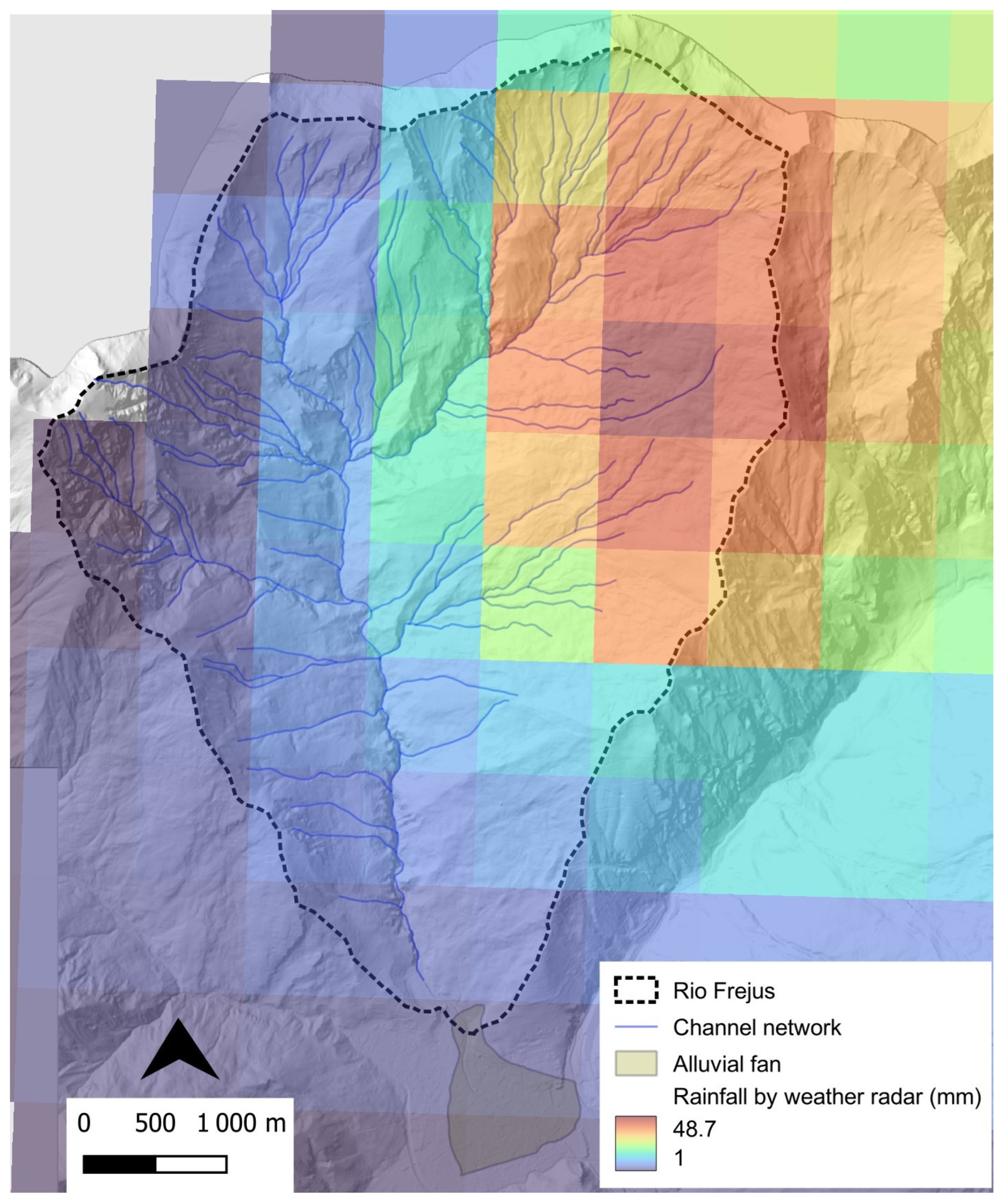
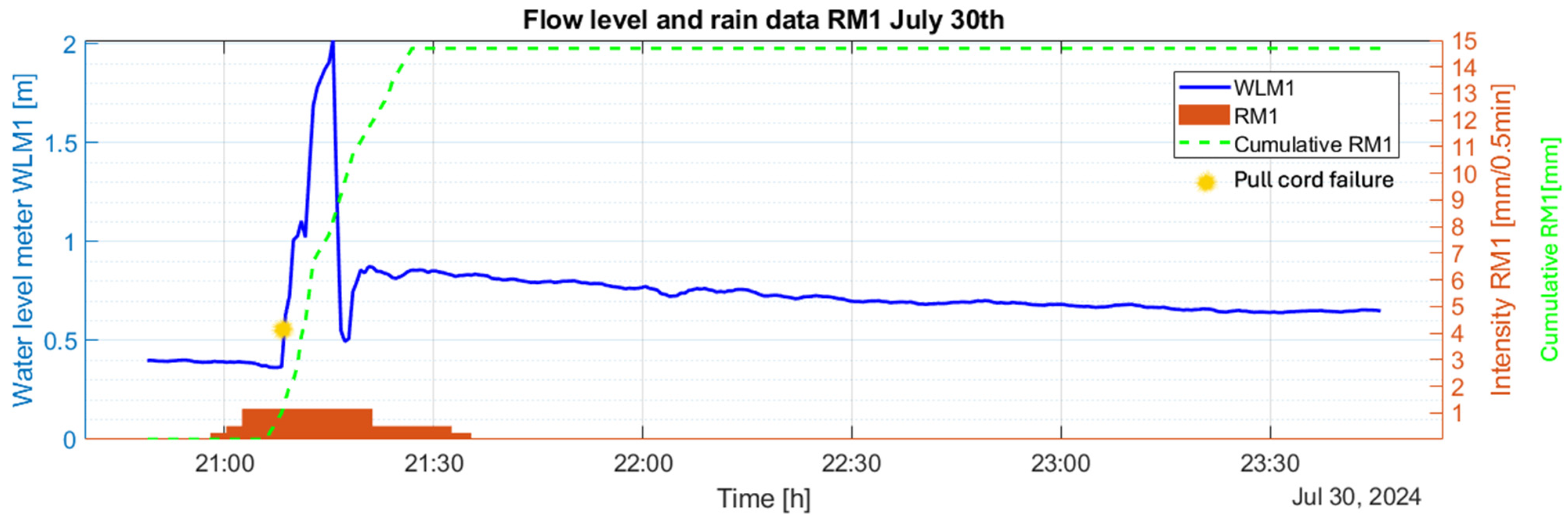
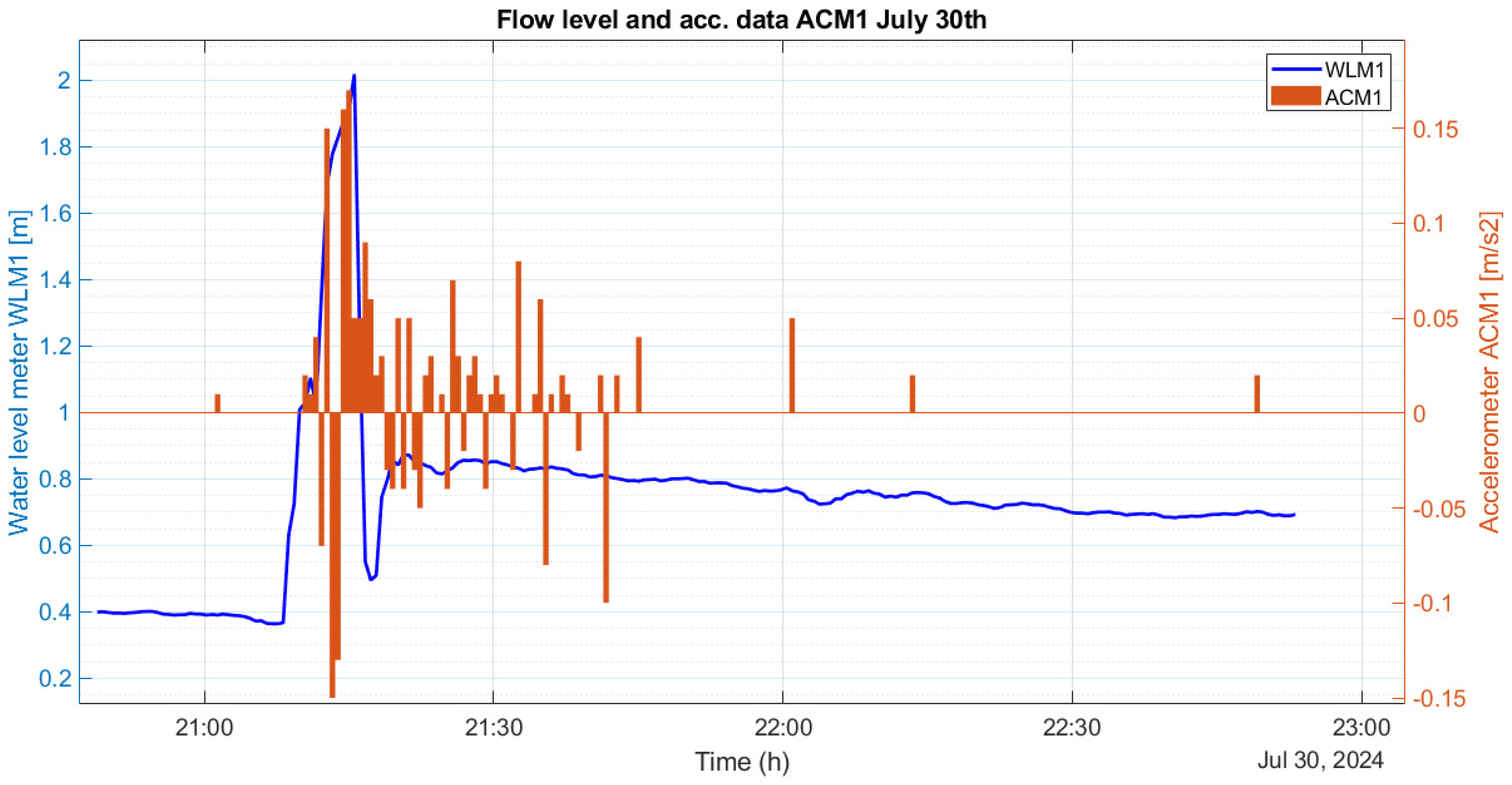
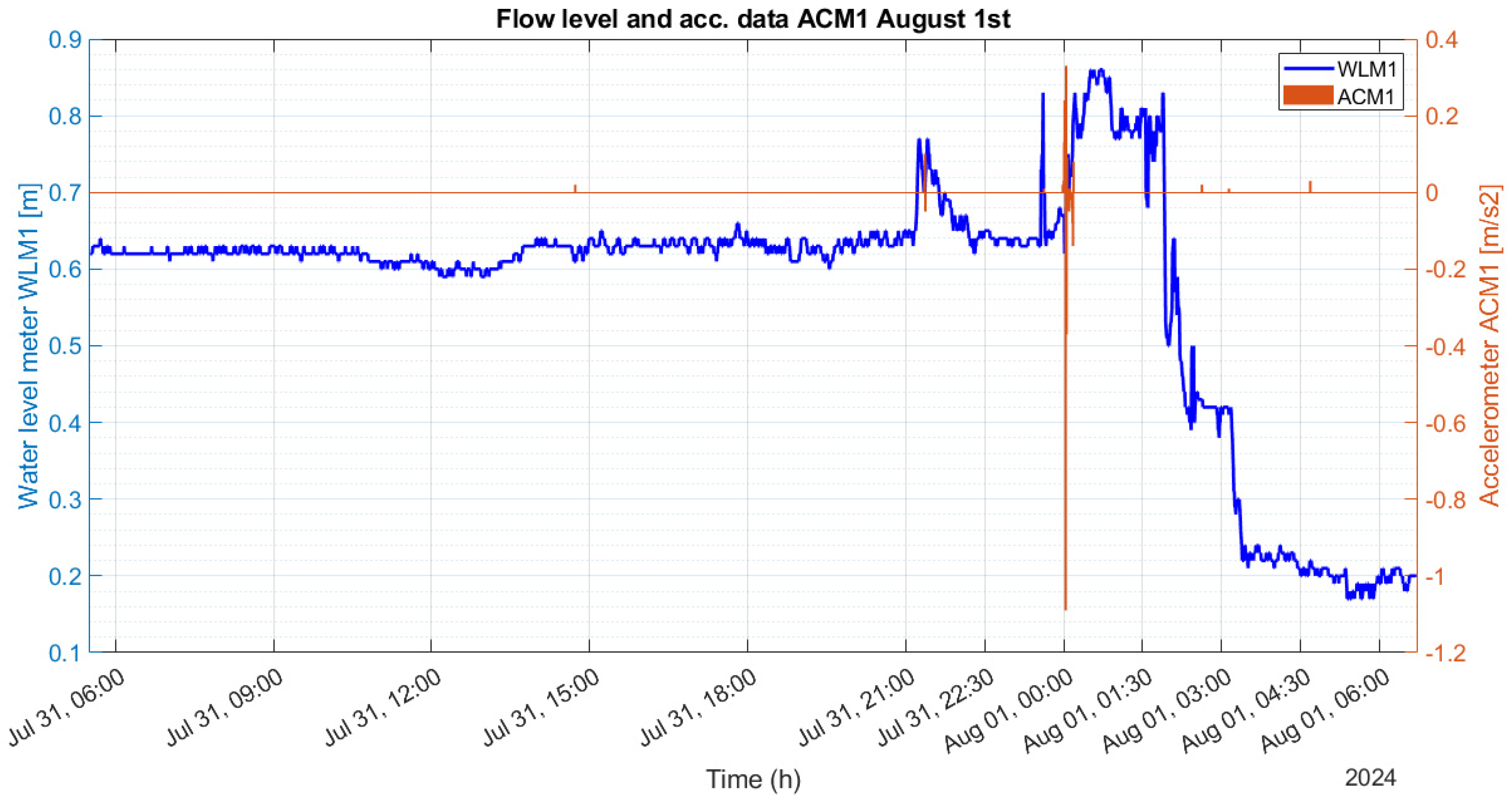
3.4. Observations Resulting from the Monitoring System

The data collected from the monitoring systems during the summer of 2024 provide a description of a series of debris flow events that occurred between 30 July and 1 August. During data processing, outliers and invalid data were filtered out to observe the flow propagation. Filtering outliers in the data involved identifying and removing erroneous data points, which were due to sensor malfunctions or other anomalies. The data were processed to remove out-of-range values, ensuring that only valid measurements were included in the analysis. Additionally, data were smoothed using a moving average technique to reduce noise and enhance the reliability of the results. The analysis of rainfall measurements prior to the event allowed for the determination of rain intensity that triggered the debris flows, although multiple factors contributed to the occurrence, such as the spatial distribution of precipitation.

To investigate the accelerometer data during the debris flow events of July and August 2024, a comparison was made with a typical flood event from the autumn season along the Rio Frejus stream. The flood event of 9 October 2024 provided a reference. The comparison between this ordinary flood event and the debris flow at the end of July revealed that only the acceleration along the y-axis was significantly higher than the values recorded during the flood, with a peak of 0.16 m/s². This result suggests that analyzing acceleration along the y-axis may be the most effective approach for detecting debris flow passage (Figure 11).

The survey area within the Merdovine sub-catchment is delineated and defined along the detachment zones near the watershed of the catchment (Figure 12). The survey campaign aimed to acquire two DEMs of the same area to compute the DEM of difference (DoD) (Figure 13). The first survey was conducted on 30 July, just prior to a significant series of debris flow events that occurred on 30 July and 31 July 2024. The second survey took place on 20 August using the same settings as the first one but with the added advantage of using the DEM obtained from the previous survey, which enabled the use of autopilot mode. For data processing purposes, the autopilot settings were configured with a longitudinal overlap of 80% and a transversal overlap of 60%.

To obtain the average thickness of deposits after the recent debris events of 30 July and 1 August at the catchment head, the DoD technique was used. This technique allows for the generation of a change map by comparing two or more digital elevation models (DEMs) acquired at different times. The map highlights the elevation differences between two or more surfaces, enabling the analysis of topographic changes over time. The DEMs used for the implementation represent the same area and were obtained from two photogrammetric surveys using UAVs. Through the process of data registration and alignment, the two models, characterized by the same spatial resolution, are georeferenced according to a common reference system and then aligned, allowing for accurate comparison. Once aligned, the difference between the two surfaces is calculated pixel by pixel. The formula is generally (Equation (6))

$$DoD=DEM\left(t_1\right)-DEM\left(t_0\right)$$

(6)

where DEM(t₁) represents the post-event terrain model, and DEM(t₀) represents the pre-event model. This results in a DoD where erosion areas will be characterized by negative values (blue color), while deposition areas will show positive values (red color in Figure 13).

The Debris Flow Events of 30 July 2024 and 1 August 2024

Between 30 July 2024 and 1 August 2024, several rainstorms affected the Frejus catchment, leading to a major debris flow event on 30 July at 09:10 P.M. This event was observed by witnesses in the center of Bardonecchia town, with some damage to the recently built hydraulic works.

On the evening of 30 July, a storm cell passed along the Cottian Alps, crossing the municipal area in a west–east direction and affecting the head of Rio Frejus catchment between 07:00 P.M. and 09:00 P.M. The storm accumulated a maximum of 48.7 mm of rain at the head of Rio Merdovine sub-catchment, as estimated by the weather radar managed by the Regional Agency for Environmental Protection of Piemonte (ARPA Piemonte) (Figure 14).

A mud–debris flow transited through the alluvial fan between 09:30 PM and 10:00 PM, depositing material in the riverbed but without overflowing (Figure 15).

Along the stream, the flow alternated between bank erosion and deposition of coarse debris and a fine fraction composed of clay, silt and sand (Figure 16A,B).

It should be noted that, during the series of debris flow events between 30 July 2024 and 1 August 2024, the monitoring network was only partially installed. Therefore, the sensors that functioned properly included PC1, WLM1, ACM1 and EQ1. Analysis of the events was based on the data recorded by these instruments.

On 31 July 2024, a new storm cell affected the Rio Frejus catchment, triggering a flow event that passed along the Rio Frejus channel between midnight and 01:00 A.M. on 1 August 2024. This event had a lower flow rate than that of 30 July, but it was sufficient to visually notice the deposits left by the previous one.

Both events were monitored by sensors, which indicated that the phenomenon only affected the Rio Merdovine sub-catchment. In fact, the WLM2 level sensor, positioned in the Rio Gautier sub-catchment, did not report significant variations. This also helped explain the small vibrations detected on weir 5 as being due to water runoff on the sensors.

Along the Rio Frejus main channel, the WLM1 level sensor detected variations in correspondence with the events but without showing the typical wave trend of debris flows in the hydrograph. This may have been due to a low sampling rate (30 s). However, in the graphs shown in Figure 17 and Figure 18, the temporal evolution of the phenomenon can still be observed.

RM1 recorded 15 mm of precipitation in less than 30 min (30 mm/h) prior to the debris flow event observation, while RM2 measured a slightly lower value of 10 mm during the same time window, corresponding to an hourly intensity of 20 mm/h. Both intensity values recorded by rain gauges were comparable with the weather radar estimation and reached the minimum triggering threshold value assigned to debris flow initiation for ECM catchments (20 mm/h), under which the Rio Frejus catchment falls. By processing the flow height values at WLM1, the characteristics of the flow and its front were extracted, showing a 1.5 m increase during the passage of the debris at 09:10 P.M. on 30 July 2024. The accelerometers recorded very high acceleration values during the same event, confirming the high energy content of the flow (Figure 19 and Figure 20).

The cross-correlation of measurements from various monitoring stations on 30 July 2024 allowed for the estimation of the transit time of the flow front and the calculation of the average flow velocity, which was approximately 2.3 m/s between ACM1 and WLM1. The observed velocity is compatible with a cohesive debris flow characterized by viscoplastic rheology, as defined by the CWI classification for ECM catchments.

The measured data confirm the behavior of flows along the channels of the Rio Frejus, as hypothesized in research works on the characterization of the catchment and its geo-hydrological processes presented in Section 3.1, Section 3.2 and Section 3.3.

4. Discussion

The results of this study emphasize the fundamental role of preliminary catchment characterization in designing an effective debris flow monitoring system.

The integration of geological, geomorphological and hydrological analyses allowed for the identification of key factors influencing debris flow initiation and propagation, which in turn allowed for a more strategic and effective placement of monitoring sensors. In particular, the classification of the Rio Frejus catchment, based on the Clay Weathering Index (CWI), the bedrock outcropping percentage method and the Debris Flow Propensity Index (DfPI), provided a solid foundation for the optimal design of the monitoring system, ensuring coverage of the most critical areas. After the system implementation and data collection began, its effectiveness became evident.

The correlation between susceptibility analyses and real-time monitoring data collected during the summer 2024 debris flow events demonstrated the system’s capacity to detect and analyze flow characteristics.

Monitoring data, along with observations in the inhabited area, confirmed that debris flows within the Rio Frejus catchment undergo a transition from cohesive debris flows to hyperconcentrated flows/mud–debris flows along the propagation path, in line with rheological predictions derived from CWI classification. This post-event validation reinforces the importance of a well-structured preliminary characterization phase.

The monitoring campaign also highlighted the crucial role of rainfall intensity thresholds in debris flow initiation. The triggering rainfall, measured by RM1 at 15 mm in 30 min, is consistent with previous studies in the Western Alps and underscores the necessity for real-time rainfall monitoring to improve predictive capabilities. The data acquired by accelerometers and seismic sensors provided further insights into flow dynamics, with acceleration peaks corresponding to debris flow fronts. These observations emphasize the value of deploying high-frequency multi-sensor systems to capture the rapid evolution of flows and enhance early warning capabilities.

Despite the demonstrated efficiency of the system, some limitations emerged. The low sampling rate (30 s) of water level sensors may have affected the resolution of hydrograph waveforms, limiting the precision of flow velocity calculations. Additionally, the monitoring network was only partially operational during the July 2024 events, reducing the completeness of data collection. Future improvements should focus on increasing sensor redundancy and enhancing data transmission to ensure more reliable real-time monitoring. However, it is important to note that such improvements should be made solely in the technological domain, as the sensor types and their distribution proved to be satisfactory.

This study also highlights the potential of integrating photogrammetry with unmanned aerial vehicles (UAVs) for event characterization. The application of the difference of digital elevation models (DoD) approach successfully quantified post-event sediment redistribution, demonstrating its utility in assessing debris flow magnitude.

Overall, the findings reinforce the necessity for a multi-disciplinary approach in designing debris flow monitoring systems to enable a timely detection of debris flow initiation despite the extent of sediment source areas and the catchment. The combination of historical, geospatial and real-time monitoring data improves risk assessment and mitigation strategies, providing a foundation for future development of an early warning system. In future research, the role of avulsion phenomena related to the propagation and deposition of debris flows [31] could also be taken into consideration to better evaluate the contribution of morphological changes in the channel network and how these can impact the performance of the monitoring network over time.

5. Conclusions

In this paper, an innovative integrated approach is presented that can best optimize the design of a monitoring system, starting from an exhaustive characterization of the catchment and the processes that occur in it.

The study therefore demonstrates its dual value, highlighting the existence of a virtuous circle in which preliminary research aimed at understanding the mechanisms that govern debris flows, i.e., the identification of predisposing and triggering factors, as well as the correct evaluation of the sediment source areas that can actually contribute to fueling such phenomena and the estimation of mobilizable sediments’ recharging time, allowed for an optimal design of a monitoring system, which, with the data acquired after its installation, allowed for the confirmation of the results deriving from preliminary research works and the actual propagation time of debris flows from the initiating areas to the alluvial fan.

This integrated study also allowed us to obtain a reliable estimate of the debris flow hazard of the Rio Frejus, and we hope that in the future, the monitoring system can be transformed into an early warning system able to guarantee timely warnings, allowing the activation of population protection measures through the issuing of alerts in the town of Bardonecchia before the flow processes reach the alluvial fan area.

References

1. Gregoretti, C.; Fontana, G. The triggering of debris flow due to channel-bed failure in some alpine headwater basins of the Dolomit6es. Analysis of critical runoff. Hydrol. Process. 2007, 22, 2248–2263. [Google Scholar] [CrossRef]
2. Dowling, C.A.; Santi, P. Debris flow and their toll on human life: A global analysis of debris flow fatalities from 1950 to 2011. Nat. Hazards 2014, 71, 203–227. [Google Scholar] [CrossRef]
3. Aaron, J.; McDougall, S.; Jordan, P. Dynamic analysis of the 2012 Johnson landslide at Kootenay Lake, British Columbia: The importance of undrained flow potential. Can. Geothech. J. 2019, 57, 1172–1182. [Google Scholar] [CrossRef]
4. Jakob, M.; McDougall, S.; Santi, P. Advances in Debris-Flow Science and Practice; Springer Nature Switzerland AG: Cham, Switzerland, 2024; 636p. [Google Scholar] [CrossRef]
5. Stoffel, M.; Tiranti, D.; Huggel, C. Climate change impacts on mass movements—Case studies from the European Alps. Sci. Total Environ. 2014, 493, 1255–1266. [Google Scholar] [CrossRef] [PubMed]
6. Vagnon, F. Design of active debris flow mitigation measures: A comprehensive analysis of existing impact models. Landslides 2020, 17, 313–333. [Google Scholar] [CrossRef]
7. Liu, K.; Wei, S. Real-time debris flow monitoring and automated warning system. J. Mt. Sci. 2024, 21, 4050–4061. [Google Scholar] [CrossRef]
8. Okuda, S.; Suwa, H.; Okunishi, K.; Yokoyama, K.; Nakano, M. Observation of the motion of debris flow and its geomorphological effects. Z. Geomorphol. 1980, 35, 142–163. [Google Scholar]
9. Berti, M.; Genevois, R.; LaHusen, R.; Simoni, A.; Tecca, P.R. Debris flow monitoring in the acquabona watershed on the Dolomites (Italian Alps). Phys. Chem. Earth (B) 2000, 25, 707–715. [Google Scholar] [CrossRef]
10. Arattano, M.; Marchi, L. Systems and Sensors for Debris-flow Monitoring and Warning. Sensors 2008, 8, 2436–2452. [Google Scholar] [CrossRef]
11. Coviello, V.; Arattano, M.; Comiti, F.; Macconi, P.; Marchi, L. Seismic Characterization of Debris Flows: Insights into Energy Radiation and Implications for Warning. J. Geophys. Res. Earth Surf. 2019, 124, 1440–1463. [Google Scholar] [CrossRef]
12. Hürlimann, M.; Coviello, V.; Bel, C.; Guo, X.; Berti, M.; Graf, G.; Hübl, J.; Miyata, S.; Smith, J.B.; Yin, H.-Y. Debris-flow monitoring and warning: Review and examples. Earth-Sci. Rev. 2019, 199, 102981. [Google Scholar] [CrossRef]
13. Cazorzi, F.; Dalla Fontana, G.; De Luca, A.; Sofia, G.; Tarolli, P. Drainage network detection and assessment of network storage capacity in agrarian landscape. Hydrol. Process. 2023, 27, 541–553. [Google Scholar] [CrossRef]
14. Hungr, O.; Morgan, G.C.; VanDine, D.F.; Lister, D.R. Debris flow defenses in British Columbia. In Debris Flows/Avalanches: Process, Recognition, and Mitigation; Costa, J.E., Wieczorek, G.F., Eds.; Geological Society of America: Boulder, CO, USA, 1987; pp. 201–222. [Google Scholar] [CrossRef]
15. Bosco, F.; Gandini, D.; Giudici, I.; Marco, F.; Paro, L.; Tararbra, M.; Tiranti, D. The Mass Movement of the Rio Frejus (Bardonecchia, NW Italian Alps) on 6 August 2004. In Evaluation and Prevention of Natural Risks; Campus, S., Barbero, S., Bovo, S., Forlati, F., Eds.; Taylor & Francis Group, Balkema: London, UK, 2007; pp. 409–447. [Google Scholar] [CrossRef]
16. Tiranti, D.; Bonetto, S.; Mandrone, G. Quantitative basin characterization to refine debris-flow triggering criteria and processes: An example from the Italian Western Alps. Landslides 2008, 5, 45–57. [Google Scholar] [CrossRef]
17. Tiranti, D.; Deangeli, C. Modeling of debris flow depositional patterns according to the catchments and sediment source areas characteristics. Front. Earth Sci. 2015, 3, 8. [Google Scholar] [CrossRef]
18. Tiranti, D.; Crema, S.; Cavalli, M.; Deangeli, C. An Integrated Study to Evaluate Debris Flow Hazard in Alpine Environment. Front. Earth Sci. 2018, 6, 60. [Google Scholar] [CrossRef]
19. Tiranti, D. Alpine Catchments’ Hazard Related to Subaerial Sediment Gravity Flows Estimated on Dominant Lithology and Outcropping Bedrock Percentage. GeoHazards 2024, 5, 652–682. [Google Scholar] [CrossRef]
20. Piana, F.; Fioraso, G.; Irace, A.; Mosca, P.; d’Atri, A.; Barale, L.; Falletti, P.; Monegato, G.; Morelli, M.; Tallone, S.; et al. Geology of Piemonte region (NW Italy, Alps–Apennines interference zone). J. Maps 2017, 13, 395–405. [Google Scholar] [CrossRef]
21. Tiranti, D.; Cremonini, R.; Marco, F.; Gaeta, A.R.; Barbero, S. The DEFENSE (DEbris Flows triggEred by storms—Nowcasting SystEm): An early warning system for torrential processes by radar storm tracking using a Geographic Information System (GIS). Comput. Geosci. 2014, 70, 96–109. [Google Scholar] [CrossRef]
22. Tiranti, D.; Cremonini, R.; Asprea, I.; Marco, F. Driving Factors for Torrential Mass-Movements Occurrence in the Western Alps. Front. Earth Sci. 2016, 4, 16. [Google Scholar] [CrossRef]
23. Bonetto, S.; Mosca, P.; Vagnon, F.; Vianello, D. New application of open source data and Rock Engineering System for debris flow susceptibility analysis. J. Mt. Sci. 2021, 18, 3200–3217. [Google Scholar] [CrossRef]
24. Vianello, D.; Vagnon, F.; Bonetto, S.; Mosca, P. Debris flow susceptibility mapping using the Rock Engineering System (RES) method: A case study. Landslides 2022, 20, 735–756. [Google Scholar] [CrossRef]
25. Hudson, J.A. Rock Engineering System: Theory and Practice; Ellis Horwood Series in Civil Engineering: New York, NY, USA, 1992; 185p. [Google Scholar]
26. Polino, R.; Dela Pierre, F.; Fioraso, G.; Giardino, M.; Gattiglio, M. Foglio 132-152-153 “Bardonecchia” Carta Geologica d’Italia, Scala 1:50,000; Servizio Geologico d’Italia: Roma, Italy, 2002. [Google Scholar]
27. Borselli, L.; Cassi, P.; Torri, D. Prolegomena to sediment and flow connectivity in the landscape: A GIS and field numerical assessment. Catena 2008, 75, 268–277. [Google Scholar] [CrossRef]
28. Cavalli, M.; Trevisani, S.; Comiti, F.; Marchi, L. Geomorphometric assessment of spatial sediment connectivity in small Alpine catchments. Geomorphology 2013, 188, 31–41. [Google Scholar] [CrossRef]
29. Crema, S.; Schenato, L.; Goldin, B.; Marchi, L.; Cavalli, M. Toward the development of a stand-alone application for the assessment of sediment connectivity. In Rendiconti Online Societa Geologica Italiana; Societa Geologica Italiana: Roma, Italy, 2015; pp. 58–61. [Google Scholar] [CrossRef]
30. Brabb, E.E. Innovative Approaches to Landslide Hazard and Risk Mapping. In International Landslide Symposium Proceedings; Landslide Society: Tokyo, Japan, 1985; Volume 1, pp. 17–22. [Google Scholar]
31. Schiavo, M.; Gregoretti, C.; Boreggio, M.; Barbini, M.; Bernard, M. Probabilistic identification of debris-flow pathways in mountain fans within a stochastic framework. J. Geophys. Res. Earth Surf. 2024, 129, e2024JF007946. [Google Scholar] [CrossRef]
Figure 1. (A) The Rio Frejus catchment and sub-catchments located in the Bardonecchia municipality (orange border). (B) The Rio Frejus synthetic geological map.
Geohazards 06 00015 g001
Figure 2. Location of the installed sensors.
Geohazards 06 00015 g002
Figure 3. Example of the monitoring sensors installed: (A) GTW2 gateway; (B) PC1 pull-cord; (C) ACM1 accelerometer and EQ1 seismic sensor; (D) ACM2 accelerometer.
Geohazards 06 00015 g003
Figure 4. Outcropping lithologies of the Rio Frejus catchment’s bedrock.
Geohazards 06 00015 g004
Figure 5. A debris flow levee deposit at the head of Rio Merdovine sub-catchment. The debris flow deposit demonstrates the nature of coarse and fine sediment fractions produced by rock weathering processes and mobilized by flow events.
Geohazards 06 00015 g005
Figure 6. (A) Surficial deposit distribution within the catchment. (B) Areas resulting from the intersection of surficial deposits and a 50 m buffer of the channel network.
Geohazards 06 00015 g006
Figure 7. The CI map of the Rio Frejus catchment—from values > −1, characterized by very high connectivity, to values < −2.9, indicating sectors with no connection—referring to the main target represented by the Rio Frejus main incised channel (modified from [18]).
Geohazards 06 00015 g007
Figure 8. Potential contribution of actual sediment source areas resulting from the intersection between surficial deposits and a 50 m buffer of the channel network (modified from [18]), with related average thickness, compared with the CI distribution representing the areas connected and disconnected from the main channel.
Geohazards 06 00015 g008
Figure 9. (A) Land use map of the Rio Frejus catchment, acquired from public repository. (B) Map of the main fracturing systems derived from aerial photo analysis and field survey.
Geohazards 06 00015 g009
Figure 10. Result of the application of RES method.
Geohazards 06 00015 g010
Figure 11. Comparison of accelerometer data on the z-axis for the flood event of 9 October and the debris flow event of 30 July.
Geohazards 06 00015 g011
Figure 12. Location of the survey area inside the Rio Merdovine sub-catchment.
Geohazards 06 00015 g012
Figure 13. The DEM of difference (DoD) derived from the difference between the DEM resulting from the first survey and the DEM resulting from the second survey. Negative values represent areas subject to erosion, while positive values represent areas of deposits. Snow blocks were excluded from the calculation.
Geohazards 06 00015 g013
Figure 14. The storm cell involved the head of Rio Frejus catchment between 07:00 P.M. and 09:00 P.M., characterized by an intensity of 24.4 mm/h, as estimated by the weather radar of ARPA Piemonte. 48.7 mm (dark-red cell on the map) corresponds to the position of the maximum value of accumulated rainfall where the main rainstorm shower affected the Rio Merdovine sub-catchment.
Geohazards 06 00015 g014
Figure 15. The mud–debris flow reached the Bardonecchia municipality (in the alluvial fan area) during the 30 July debris flow event.
Geohazards 06 00015 g015
Figure 16. (A) Debris flow initiation area at the head of the Rio Merdovine sub-catchment. (B) Traces of the passage of debris flow just upstream of the confluence between the Rio Merdovine and the Rio Frejus main channel.
Geohazards 06 00015 g016
Figure 17. Comparison between the values recorded by the RM1 rain gauge and the level values measured in the Rio Frejus channel through WLM1 between 30 July and 31 July.
Geohazards 06 00015 g017
Figure 18. Comparison between the values recorded by the RM2 rain gauge and the level values measured in the Rio Frejus channel through WLM1 between 31 July and 1 August.
Geohazards 06 00015 g018
Figure 19. Comparison between the values recorded by the ACM1 accelerometer along the z-axis and the level values measured in the Rio Frejus channel through WLM1 between 30 and 31 July.
Geohazards 06 00015 g019
Figure 20. Comparison between the values recorded by the ACM1 accelerometer along the z-axis and the level values measured in the Rio Frejus channel through WLM1 between 31 July and 1 August.
Geohazards 06 00015 g020