
The Destabilizing Effect of Glacial Unloading on a Large Volcanic Slope Instability in Southeast Iceland

 , , , ,
Abstract
1. Introduction
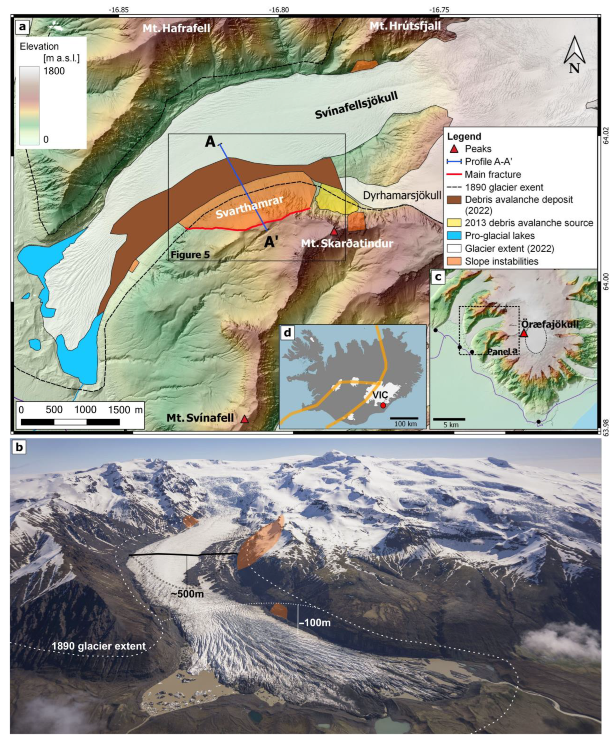
Study Area
2. Methods
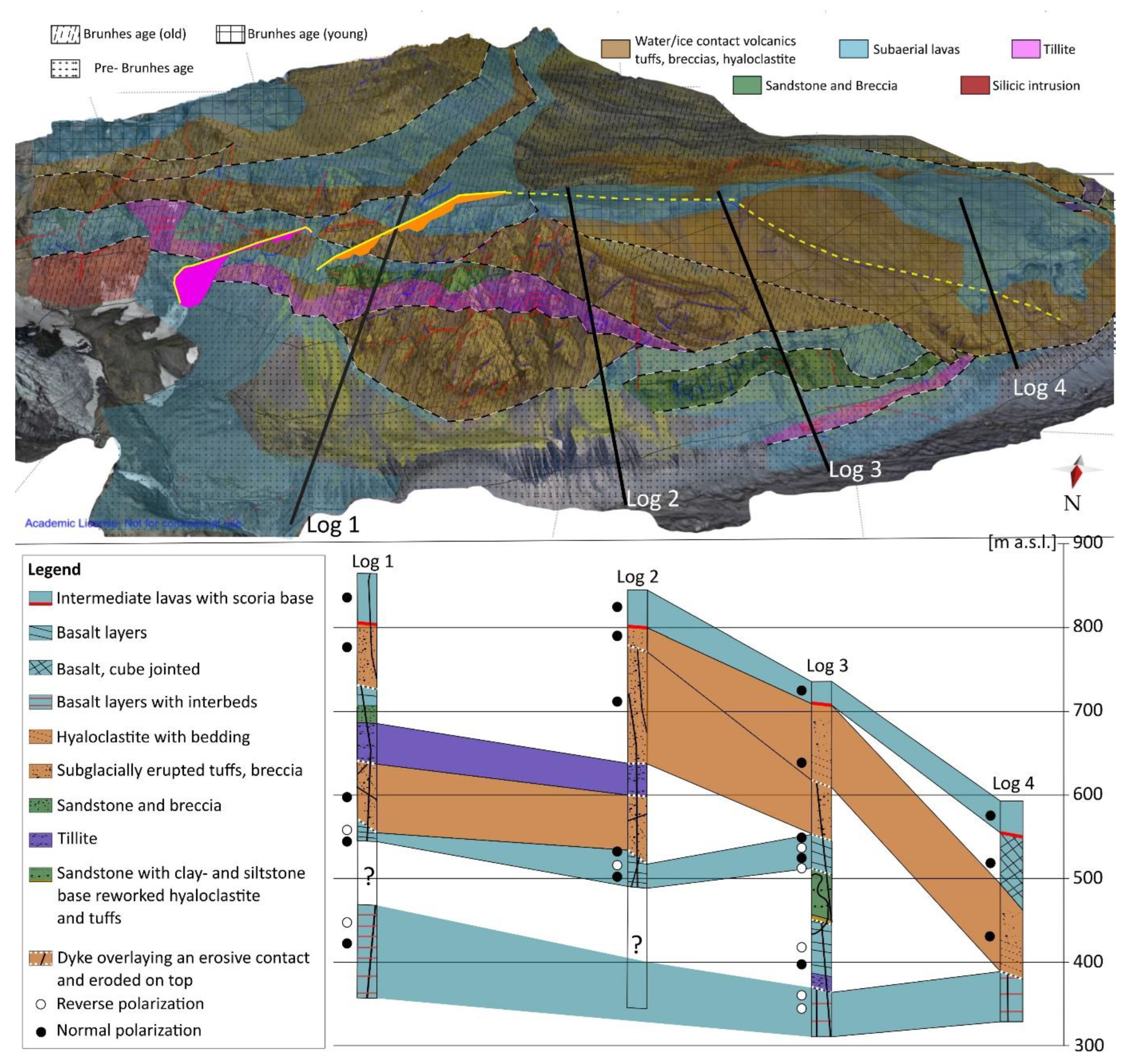
2.1. Geological and Structural Mapping
2.2. Radio Echo Sounding and Glacier Bed
2.3. Stability Modelling
2.3.1. Stratigraphic Units and Model Parameters
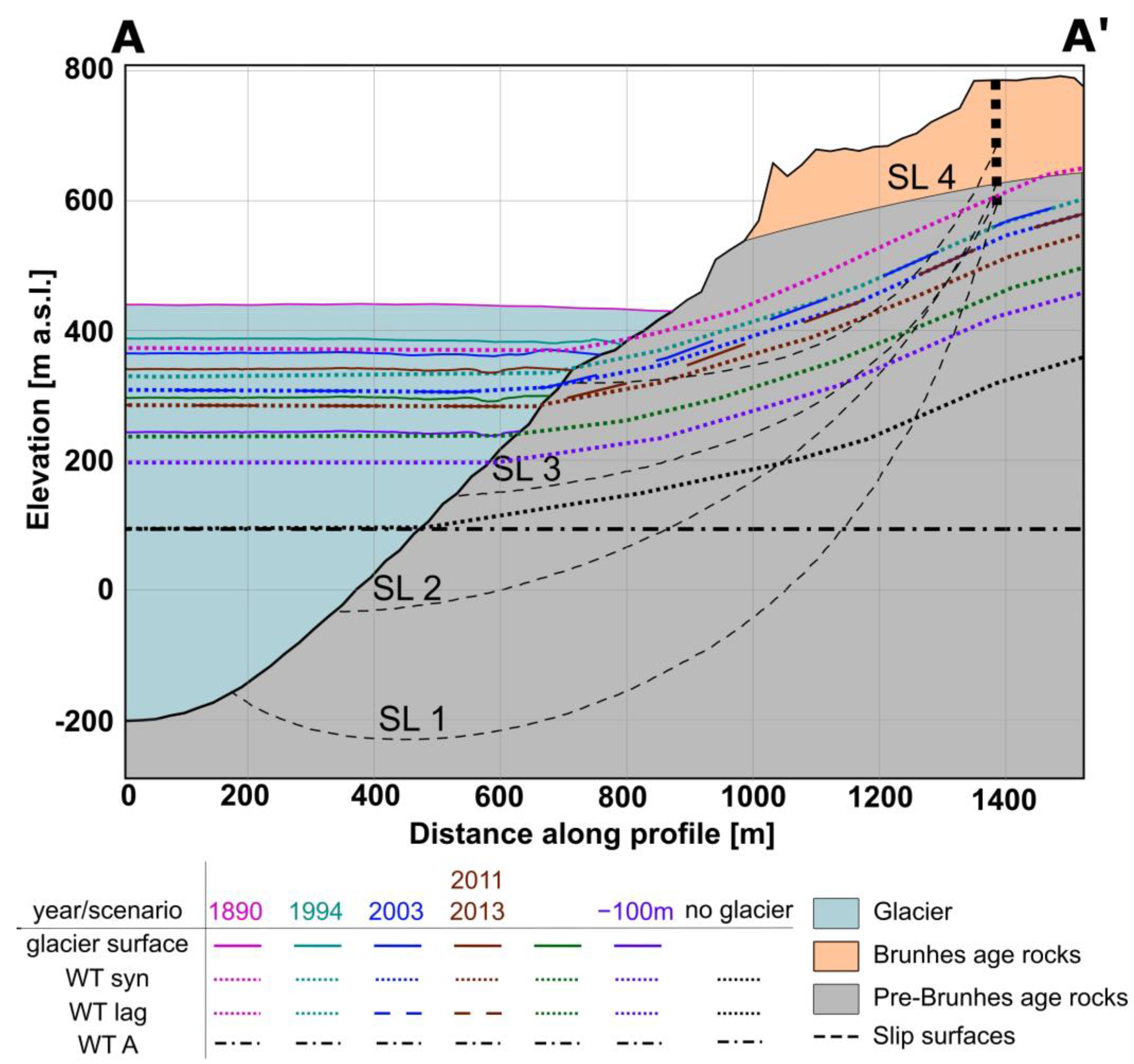
2.3.2. Slip Surfaces
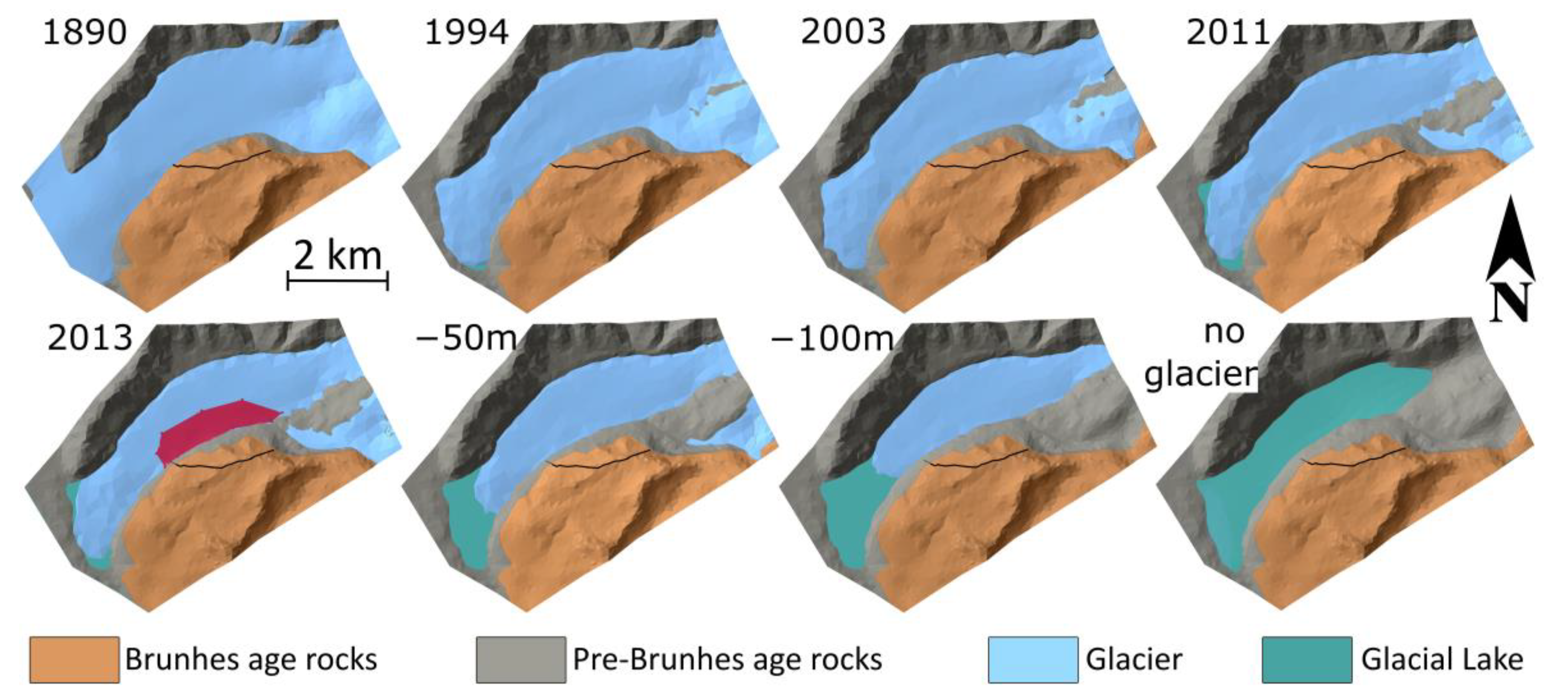
2.3.3. Glacier Scenarios
2.3.4. Water Surfaces
2.3.5. Seismic Scenarios
3. Results
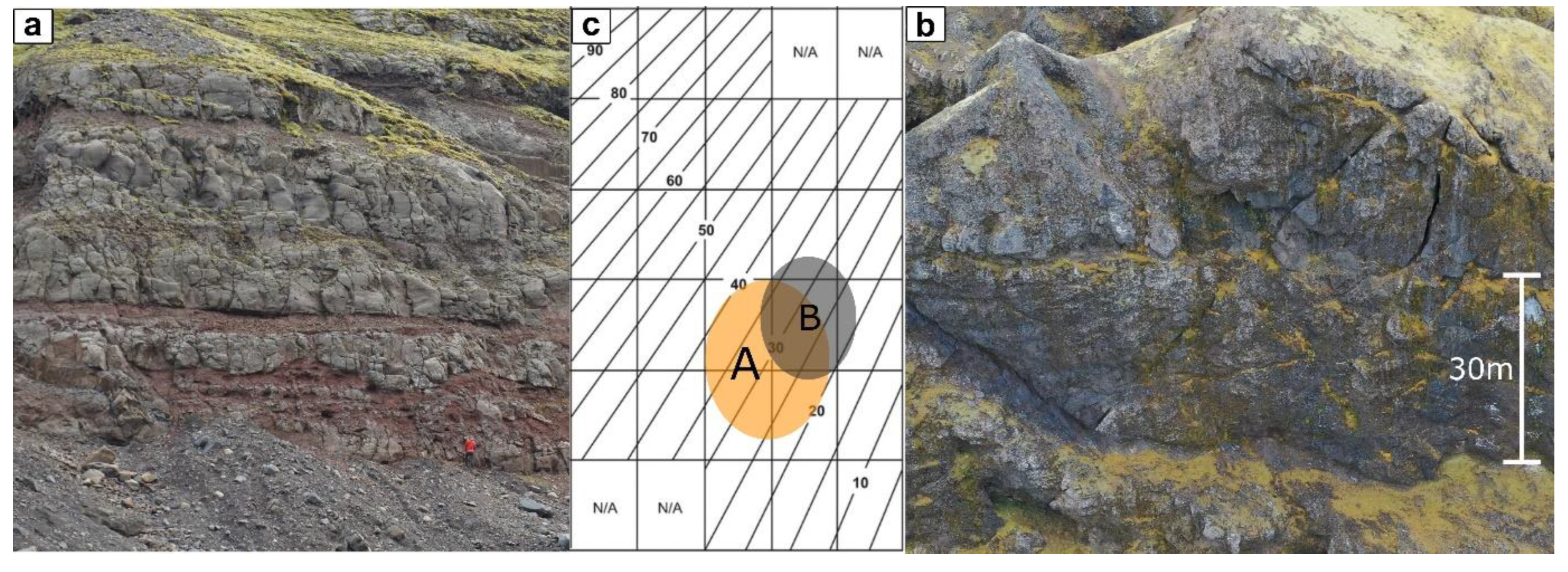
3.1. Geology and Important Structures
3.2. Structural Observations
3.3. Modelling Results
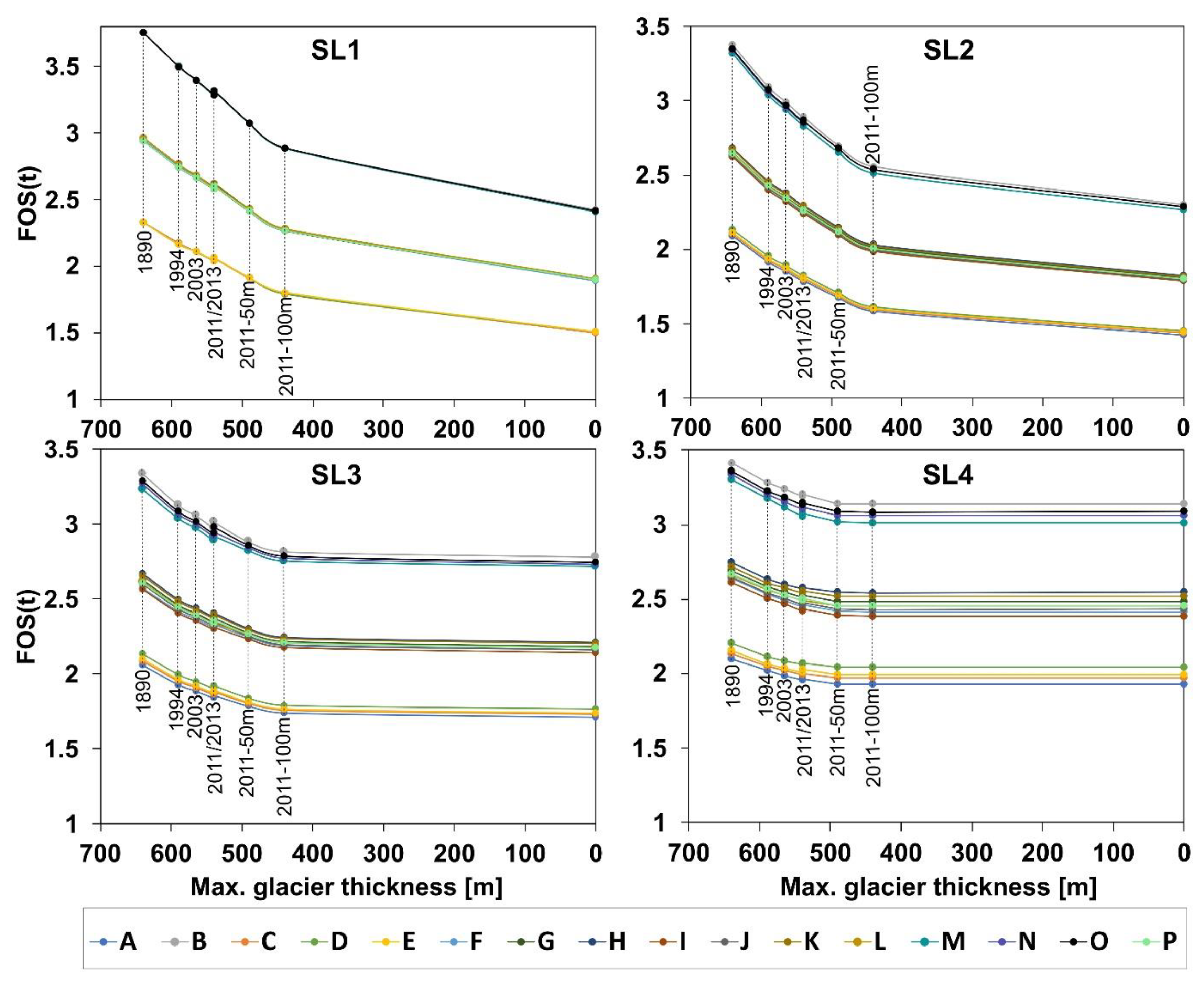
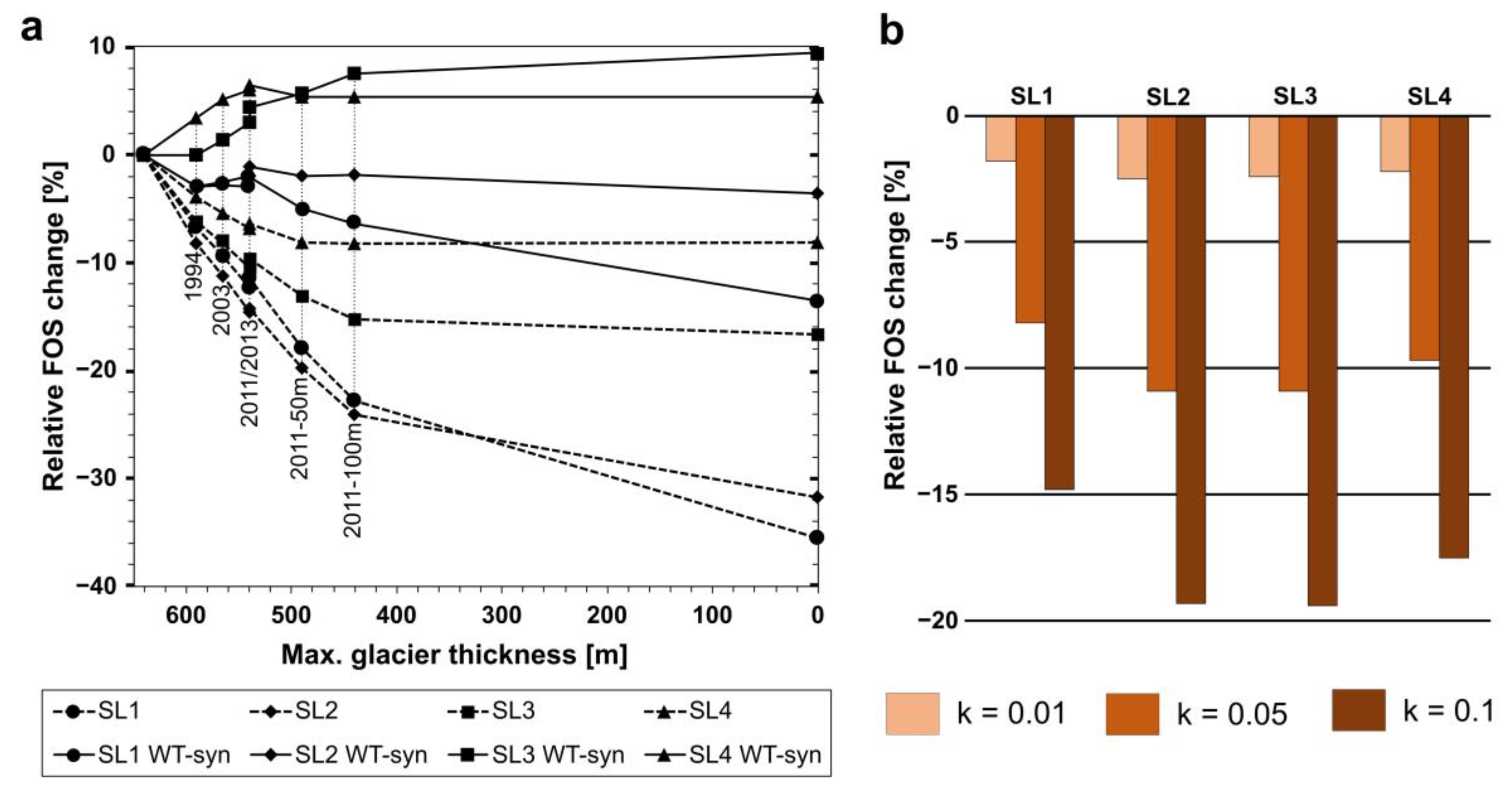
3.3.1. Scenarios A–P
3.3.2. Seismic Acceleration
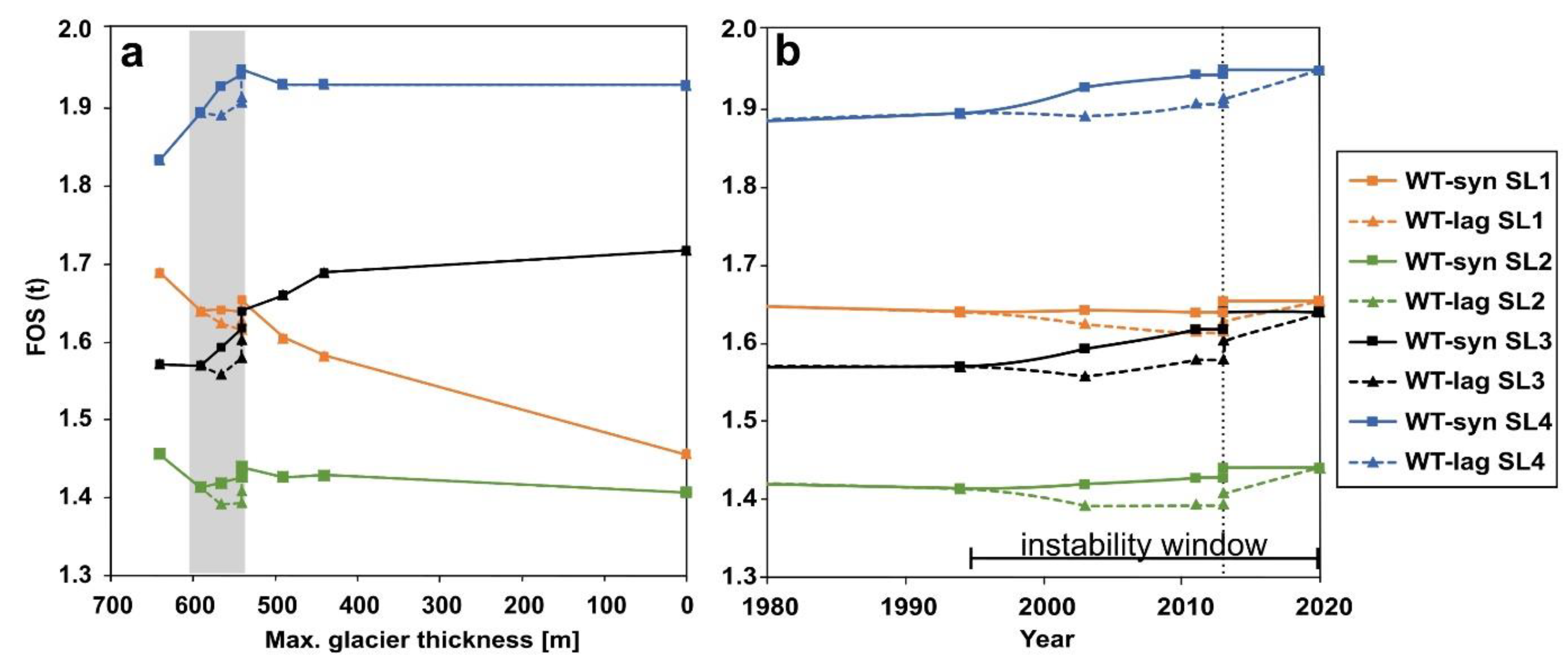
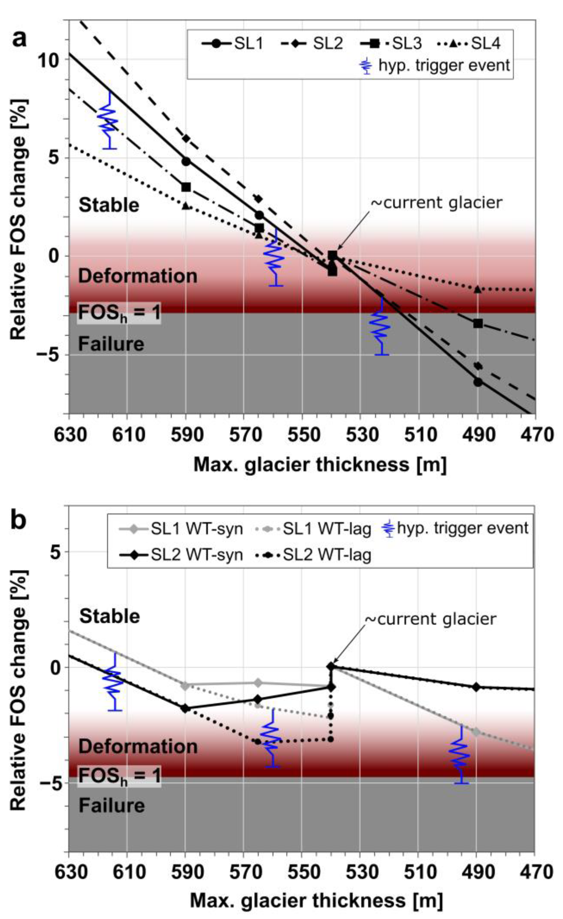
3.3.3. Scenarios WT-syn and WT-lag
4. Discussion
4.1. Geology and Important Structures
4.2. Scenarios A–P and Seismic Acceleration
4.3. Interpretation of WT-syn and WT-lag
4.4. Wider Implications
5. Conclusions
Supplementary Materials
Author Contributions
Funding
Data Availability Statement
Acknowledgments
Conflicts of Interest
References
- Hugonnet, R.; McNabb, R.; Berthier, E.; Menounos, B.; Nuth, C.; Girod, L.; Farinotti, D.; Huss, M.; Dussaillant, I.; Brun, F.; et al. Accelerated Global Glacier Mass Loss in the Early Twenty-First Century. Nature 2021, 592, 726–731. [Google Scholar] [CrossRef] [PubMed]
- Zemp, M.; Huss, M.; Thibert, E.; Eckert, N.; McNabb, R.; Huber, J.; Barandun, M.; Machguth, H.; Nussbaumer, S.U.; Gärtner-Roer, I.; et al. Global Glacier Mass Changes and Their Contributions to Sea-Level Rise from 1961 to 2016. Nature 2019, 568, 382–386. [Google Scholar] [CrossRef]
- Meredith, M.; Sommerkorn, M.; Cassotta, S.; Derksen, C.; Ekaykin, A.; Hollowed, A.; Kofinas, G.; Mackintosh, A.; Melbourne-Thomas, J.; Muelbert, M.M.C.; et al. Polar Regions. In IPCC Special Report on the Ocean and Cryosphere in a Changing Climate; IPCC: Geneva, Switzerland, 2019; pp. 203–320. [Google Scholar]
- Ballantyne, C.K. Paraglacial Geomorphology. In Reference Module in Earth Systems and Environmental Sciences; Elsevier Inc.: Amsterdam, The Netherlands, 2022; pp. 1–22. ISBN 9780323999311. [Google Scholar]
- McColl, S.T.; Draebing, D. Rock Slope Instability in the Proglacial Zone: State of the Art. In Geomorphology of Proglacial Systems: Landform and Sediment Dynamics in Recently Deglaciated Alpine Landscapes; Springer: Cham, Switzerland, 2019; pp. 119–141. [Google Scholar] [CrossRef]
- Ballantyne, C.K.; Sandeman, G.F.; Stone, J.O.; Wilson, P. Rock-Slope Failure Following Late Pleistocene Deglaciation on Tectonically Stable Mountainous Terrain. Quat. Sci. Rev. 2014, 86, 144–157. [Google Scholar] [CrossRef]
- Hermanns, R.L.; Schleier, M.; Böhme, M.; Blikra, L.H.; Gosse, J.; Ivy-Ochs, S.; Hilger, P. Rock-Avalanche Activity in W and S Norway Peaks after the Retreat of the Scandinavian Ice Sheet. In Proceedings of the 4th World Landslide Forum, Ljubljana, Slovenia, 30 May–2 June 2017; pp. 331–338. [Google Scholar]
- Böhme, M.; Oppikofer, T.; Longva, O.; Jaboyedoff, M.; Hermanns, R.L.; Derron, M.H. Analyses of Past and Present Rock Slope Instabilities in a Fjord Valley: Implications for Hazard Estimations. Geomorphology 2015, 248, 464–474. [Google Scholar] [CrossRef]
- Mercier, D.; Coquin, J.; Feuillet, T.; Decaulne, A.; Cossart, E.; Jónsson, H.P.; Sæmundsson, Þ. Are Icelandic Rock-Slope Failures Paraglacial? Age Evaluation of Seventeen Rock-Slope Failures in the Skagafjörður Area, Based on Geomorphological Stacking, Radiocarbon Dating and Tephrochronology. Geomorphology 2017, 296, 45–58. [Google Scholar] [CrossRef]
- Hermanns, R.L.; Niedermann, S.; Villanueva, G.A.; Schellenberger, A. Rock Avalanching in the NW Argentine Andes as a Result of Complex Interactions of Lithologic, Structural and Topographic Boundary Conditions, Climate Change and Active Tectonics. In Landslides from Massive Rock Slope Failure, Proceedings of the NATO Advanced Research Workshop on Massive Rock Slope Failure—New Models for Hazard Assessment; Springer: Berlin/Heidelberg, Germany, 2006; pp. 497–520. [Google Scholar]
- González-Díez, A.; Remondo, J.; Díaz De Terán, J.R.; Cendrero, A. A Methodological Approach for the Analysis of the Temporal Occurrence and Triggering Factors of Landslides. Geomorphology 1999, 30, 95–113. [Google Scholar] [CrossRef]
- Evans, S.G.; Clague, J.J. Recent Climatic Change and Catastrophic Geomorphic Processes in Mountain Environments. Geomorphol. Nat. Hazards 1994, 10, 107–128. [Google Scholar] [CrossRef]
- Grämiger, L.M.; Moore, J.R.; Gischig, V.S.; Loew, S. Thermomechanical Stresses Drive Damage of Alpine Valley Rock Walls during Repeat Glacial Cycles. J. Geophys. Res. Earth Surf. 2018, 123, 2620–2646. [Google Scholar] [CrossRef]
- Grämiger, L.M.; Moore, J.R.; Gischig, V.S.; Loew, S.; Funk, M.; Limpach, P. Hydromechanical Rock Slope Damage during Late Pleistocene and Holocene Glacial Cycles in an Alpine Valley. J. Geophys. Res. Earth Surf 2020, 125, e2019JF005494. [Google Scholar] [CrossRef]
- Grämiger, L.M.; Moore, J.R.; Gischig, V.S.; Ivy-Ochs, S.; Loew, S. Beyond Debuttressing: Mechanics of Paraglacial Rock Slope Damage during Repeat Glacial Cycles. J. Geophys. Res. Earth Surf. 2017, 122, 1004–1036. [Google Scholar] [CrossRef]
- Miles, K.E.; Hubbard, B.; Irvine-Fynn, T.D.L.; Miles, E.S.; Quincey, D.J.; Rowan, A.V. Hydrology of Debris-Covered Glaciers in High Mountain Asia. Earth Sci. Rev. 2020, 207, 103212. [Google Scholar] [CrossRef]
- Eberhardt, E.; Stead, D.; Coggan, J.S. Numerical Analysis of Initiation and Progressive Failure in Natural Rock Slopes-the 1991 Randa Rockslide. Int. J. Rock Mech. Min. Sci. 2004, 41, 69–87. [Google Scholar] [CrossRef]
- Stead, D.; Eberhardt, E. Understanding the Mechanics of Large Landslides. Ital. J. Eng. Geol. Environ.-Book Ser. 2013, 6, 85–112. [Google Scholar] [CrossRef]
- Jaboyedoff, M.; Baillifard, F.; Bardou, E.; Girod, F. The Effect of Weathering on Alpine Rock Instability. Q. J. Eng. Geol. Hydrogeol. 2004, 37, 95–103. [Google Scholar] [CrossRef]
- Glen, J.W. The Flow Law of Ice: A Discussion of the Assumptions Made in Glacier Theory, Their Experimental Foundations and Consequences. IASH Publ. 1958, 47, 171–183. [Google Scholar]
- Schulson, E.M. Brittle Failure of Ice. Eng. Fract. Mech. 2001, 68, 1839–1887. [Google Scholar] [CrossRef]
- McColl, S.T.; Davies, T.R.H. Large Ice-Contact Slope Movements: Glacial Buttressing, Deformation and Erosion. Earth Surf. Process. Landf. 2013, 38, 1102–1115. [Google Scholar] [CrossRef]
- McColl, S.T.; Davies, T.; McSaveney, M.J. Glacier Retreat and Rock-Slope Stability: Debunking Debuttressing. In Proceedings of the Geologically Active: Delegate Papers 11th Congress of the International Association for Engineering Geology and the Environment, Auckland, New Zealand, 5–10 September 2010; pp. 467–474. [Google Scholar]
- Storni, E.; Hugentobler, M.; Manconi, A.; Loew, S. Monitoring and Analysis of Active Rockslide-Glacier Interactions (Moosfluh, Switzerland). Geomorphology 2020, 371, 107414. [Google Scholar] [CrossRef]
- Ben-Yehoshua, D.; Sæmundsson, Þ.; Erlingsson, S.; Helgason, J.K.; Hermanns, R.L.; Magnússon, E.; Ófeigsson, B.G.; Belart, J.M.C.; Hjartardóttir, Á.R.; Geirsson, H.; et al. The Destabilization of a Large Mountain Slope Controlled by Thinning of Svínafellsjökull Glacier, SE Iceland. Jökull 2023, 1–33. [Google Scholar] [CrossRef]
- Cuffey, K.M.; Paterson, W.S.B. The Physics of Glaciers, 4th ed.; Elsevier: Amsterdam, The Netherlands, 2010. [Google Scholar]
- Hugentobler, M.; Aaron, J.; Loew, S.; Roques, C. Hydro-Mechanical Interactions of a Rock Slope with a Retreating Temperate Valley Glacier. J. Geophys. Res. Earth Surf. 2022, 127, 1–31. [Google Scholar] [CrossRef]
- Burns, E.R.; Williams, C.F.; Ingebritsen, S.E.; Voss, C.I.; Spane, F.A.; Deangelo, J. Understanding Heat and Groundwater Flow through Continental Flood Basalt Provinces: Insights Gained from Alternative Models of Permeability/Depth Relationships for the Columbia Plateau, United States. In Crustal Permeability; Wiley: Hoboken, NJ, USA, 2016; pp. 137–154. [Google Scholar] [CrossRef]
- Dijksma, R.; Avis, L. Measuring and Modelling Water Transport on Skaftafellsheiði, Iceland. Forum Geogr. 2016, 15, 66–72. [Google Scholar] [CrossRef]
- Faybishenko, B.; Doughty, C.; Steiger, M.; Long, J.C.S.; Wood, T.R.; Jacobsen, J.S.; Lore, J.; Zawislanski, P. Conceptual Model of the Geometry and Physics of Water Flow in a Fractured Basalt Vadose Zone. Water Resour. Res. 2000, 36, 3499–3520. [Google Scholar] [CrossRef]
- Terzaghi, K. Stability of Steep Slopes on Hard Unweathered Rock. Geotechnique 1962, 12, 251–270. [Google Scholar] [CrossRef]
- van Wyk de Vries, B.; Davies, T. Landslides, Debris Avalanches, and Volcanic Gravitational Deformation, 2nd ed.; Elsevier Inc.: Amsterdam, The Netherlands, 2015; Volume 1, ISBN 9780123859389. [Google Scholar]
- Roverato, M.; Dufresne, A.; Procter, J. Volcanic Debris Avalanches from Collapse to Hazard; Springer: Cham, Switzerland, 2021; ISBN 9783030574109. [Google Scholar]
- Dufresne, A.; Siebert, L.; Bernard, B. Distribution and Geometric Parameters of Volcanic Debris Avalanche Deposits; Springer International Publishing: Berlin/Heidelberg, Germany, 2021; ISBN 9783030574116. [Google Scholar]
- Glicken, H. Rockslide-Debris Avalanche of May 18, 1980, Mount St. Helens Volcano, Washington. U.S. Geol. Surv. Open-File Rep. 1996, 96, 1–90. [Google Scholar]
- Roberti, G.; Ward, B.; van Wyk de Vries, B.; Falorni, G.; Menounos, B.; Friele, P. Landslides and Glacier Retreat at Mt. Meager Volcano: Hazard and Risk Challenges. In Proceedings of the 7th Canadian Geohazards Conference: Engineering Resiliency in a Changing Climate, Canmore, AB, Canada, 3–6 June 2018. [Google Scholar]
- Svennevig, K.; Owen, M.J.; Citterio, M.; Nielsen, T.; Rosing, S.; Harff, J.; Endler, R.; Morlighem, M.; Rignot, E. Holocene Gigascale Rock Avalanches in Vaigat Strait, West Greenland—Implications for Geohazard. Geology 2024, 52, 147–152. [Google Scholar] [CrossRef]
- Pánek, T.; Břežný, M.; Smedley, R.; Winocur, D.; Schönfeldt, E.; Agliardi, F.; Fenn, K. The Largest Rock Avalanches in Patagonia: Timing and Relation to Patagonian Ice Sheet Retreat. Quat. Sci. Rev. 2023, 302, 107962. [Google Scholar] [CrossRef]
- Kjartansson, G. Steinsholtshlaup, Central-South Iceland on January 15th, 1967. Jökull 1967, 17, 249–262. [Google Scholar] [CrossRef]
- Jónsson, Ó.B. Berghlaup; Prentverk Odds Björnssonar hf.: Akureyri, Iceland, 1974. (In Icelandic) [Google Scholar]
- Cossart, E.; Mercier, D.; Decaulne, A.; Feuillet, T.; Jónsson, H.P.; Sæmundsson, Þ. Impacts of Post-Glacial Rebound on Landslide Spatial Distribution at a Regional Scale in Northern Iceland (Skagafjörður). Earth Surf. Process. Landf. 2014, 39, 336–350. [Google Scholar] [CrossRef]
- Whalley, W.B.; Douglas, G.R.; Jonsson, A. The Magnitude and Frequency of Large Rockslides in Iceland in the Postglacial. Geogr. Annaler. Ser. A Phys. Geogr. 1983, 65, 99. [Google Scholar] [CrossRef]
- Aðalgeirsdóttir, G.; Magnússon, E.; Pálsson, F.; Thorsteinsson, T.; Belart, J.M.C.; Jóhannesson, T.; Hannesdóttir, H.; Sigurðsson, O.; Gunnarsson, A.; Einarsson, B.; et al. Glacier Changes in Iceland from ~1890 to 2019. Front. Earth Sci. 2020, 8, 574754. [Google Scholar] [CrossRef]
- Hannesdóttir, H.; Björnsson, H.; Pálsson, F.; Aðalgeirsdóttir, G.; Guðmundsson, S. Changes in the Southeast Vatnajökull Ice Cap, Iceland, between ∼1890 and 2010. Cryosphere 2015, 9, 565–585. [Google Scholar] [CrossRef]
- Hannesdóttir, H.; Sigurðsson, O.; Þrastarson, R.H.; Guðmundsson, S.; Belart, J.M.C.; Pálsson, F.; Magnússon, E.; Víkingsson, S.; Kaldal, I.; Jóhannesson, T. A National Glacier Inventory and Variations in Glacier Extent in Iceland from the Little Ice Age Maximum to 2019. Jokull 2020, 2020, 1–34. [Google Scholar] [CrossRef]
- Belart, J.M.C.; Magnússon, E.; Berthier, E.; Gunnlaugsson, Á.; Pálsson, F.; Aðalgeirsdóttir, G.; Jóhannesson, T.; Thorsteinsson, T.; Björnsson, H. Mass Balance of 14 Icelandic Glaciers, 1945–2017: Spatial Variations and Links with Climate. Front. Earth Sci. 2020, 8, 163. [Google Scholar] [CrossRef]
- Einarsson, P. Plate Boundaries, Rifts and Transforms in Iceland. Jökull 2008, 58, 35–58. [Google Scholar] [CrossRef]
- Sólnes, J.; Sigbjörnsson, R.; Elíasson, J. Probabilistic Seismic Hazard Mapping of Iceland. Proposed Seismic Zoning and de-Aggregation Mapping for EUROCODE 8. In Proceedings of the 13th World Conference on Earthquake Engineering (13WCEE), Vancouver, BC, Canada, 1–6 August 2004. Paper No. 2337. [Google Scholar]
- Einarsson, P. Historical Accounts of Pre-Eruption Seismicity of Katla, Hekla, Öræfajökull and Other Volcanoes in Iceland. Jökull 2019, 69, 35–52. [Google Scholar] [CrossRef]
- Geirsson, H.; Parks, M.M.; Ófeigsson, B.G.; Drouin, V.; Li, S.; Sigmundsson, F.; Árnadóttir, T.; Hjartardottir, A.R.; Lárentínusdóttir, M.; Einarsson, P.; et al. Reawakening of the Öræfajökull Volcano in Iceland: Deformation Signals of Stress Triggers and Intrusive Activity. In EGU General Assembly Conference Abstracts; EGU: Munich, Germany, 2018; p. 15438. [Google Scholar]
- Guðmundsson, H.J. Holocene Glacier Fluctuations and Tephrochronology of the Öræfi District, Iceland. Ph.D. Thesis, University of Edinburgh, Edinburgh, Scotland, 1998. [Google Scholar]
- Ben-Yehoshua, D.; Sæmundsson, Þ.; Helgason, J.K.; Belart, J.M.C.; Sigurðsson, J.V.; Erlingsson, S. Paraglacial Exposure and Collapse of Glacial Sediment: The 2013 Landslide onto Svínafellsjökull, Southeast Iceland. Earth Surf. Process. Landf. 2022, 47, 2612–2627. [Google Scholar] [CrossRef]
- Crochet, P. A Study of Regional Precipitation Trends in Iceland Using a High-Quality Gauge Network and ERA-40. J. Clim. 2007, 20, 4659–4677. [Google Scholar] [CrossRef]
- Sæmundsson, Þ.; Pétursson, H.G.; Decaulne, A. Triggering Factors for Rapid Mass Movements in Iceland. Int. Conf. Debris-Flow Hazards Mitig. Mech. Predict. Assess. Proc. 2003, 1, 167–178. [Google Scholar]
- Helgason, J.; Duncan, R.A. Stratigraphy, 40Ar–39Ar Dating and Erosional History of Svínafell, SE-Iceland. Jökull 2013, 63, 33–54. [Google Scholar] [CrossRef]
- Helgason, J.; Duncan, R.A. Magnetostratigraphy, K-Ar Dating and Erosion History of the Hafrafell Volcanics, SE–Iceland. Jökull 2014, 64, 41–60. [Google Scholar] [CrossRef]
- Lee, R.E.; Maclachlan, J.C.; Eyles, C.H. Landsystems of Morsárjökull, Skaftafellsjökull and Svínafellsjökull, Outlet Glaciers of the Vatnajökull Ice Cap, Iceland. Boreas 2018, 47, 1199–1217. [Google Scholar] [CrossRef]
- Everest, J.; Bradwell, T.; Jones, L.; Hughes, L. The Geomorphology of Svínafellsjökull and Virkisjökull-Falljökull Glacier Forelands, Southeast Iceland. J. Maps 2017, 13, 936–945. [Google Scholar] [CrossRef]
- Thompson, A. Historical Development of the Proglacial Landforms of Svínafellsjökull and Skaftafellsjökull, Southeast Iceland. Jökull 1988, 38, 17–30. [Google Scholar] [CrossRef]
- Helgason, J.; Duncan, R.A. Glacial-Interglacial History of the Skaftafell Region, Southeast Iceland, 0–5 Ma. Geology 2001, 29, 179–182. [Google Scholar] [CrossRef]
- Primdahl, F. The Fluxgate Magnetometer. J. Phys. E 1979, 12, 241–253. [Google Scholar] [CrossRef]
- Singer, B.S. A Quaternary Geomagnetic Instability Time Scale. Quat. Geochronol. 2014, 21, 29–52. [Google Scholar] [CrossRef]
- Jóhannesson, T.; Björnsson, H.; Magnússon, E.; Guðmundsson, S.; Pálsson, F.; Sigurðsson, O.; Thorsteinsson, T.; Berthier, E. Ice-Volume Changes, Bias Estimation of Mass-Balance Measurements and Changes in Subglacial Lakes Derived by Lidar Mapping of the Surface of Icelandic Glaciers. Ann. Glaciol. 2013, 54, 63–74. [Google Scholar] [CrossRef]
- Magnússon, E.; Pálsson, F.; Björnsson, H.; Gudmundsson, S. Removing the Ice Cap of Öræfajökull Central Volcano, SE-Iceland: Mapping and Interpretation of Bedrock Topography, Ice Volumes, Subglacial Troughs and Implications for Hazards Assessments. Jökull 2014, 64, 83–84. [Google Scholar] [CrossRef]
- Mingo, L.; Flowers, G.E. Instruments and Methods An Integrated Lightweight Ice-Penetrating Radar System. J. Glaciol. 2010, 56, 709–714. [Google Scholar] [CrossRef]
- Magnússon, E.; Pálsson, F.; Gudmundsson, M.T.; Högnadóttir, T.; Rossi, C.; Thorsteinsson, T.; Ófeigsson, B.G.; Sturkell, E.; Jóhannesson, T. Development of a Subglacial Lake Monitored with Radio-Echo Sounding: Case Study from the Eastern Skaftá Cauldron in the Vatnajökull Ice Cap, Iceland. Cryosphere 2021, 15, 3731–3749. [Google Scholar] [CrossRef]
- Bradford, J.H.; Nichols, J.; Mikesell, T.D.; Harper, J.T. Continuous Profiles of Electromagnetic Wave Velocity and Water Content in Glaciers: An Example from Bench Glacier, Alaska, USA. Ann. Glaciol. 2009, 50, 1–9. [Google Scholar] [CrossRef]
- Duncan, J.M. Factors of Safety and Reliability in Geotechnical Engineering. J. Geotech. Geoenviron. Eng. 2000, 126, 307–316. [Google Scholar] [CrossRef]
- Hoek, E.; Brown, E.T. The Hoek–Brown Failure Criterion and GSI—2018 Edition. J. Rock Mech. Geotech. Eng. 2019, 11, 445–463. [Google Scholar] [CrossRef]
- Scott, S.W.; Lévy, L.; Covell, C.; Franzson, H.; Gibert, B.; Valfells, Á.; Newson, J.; Frolova, J.; Júlíusson, E.; Guðjónsdóttir, M.S. Valgarður: A Database of the Petrophysical, Mineralogical, and Chemical Properties of Icelandic Rocks. Earth Syst. Sci. Data 2023, 15, 165–1195. [Google Scholar] [CrossRef]
- Loftsson, M.; Jóhannsson, Æ.; Erlingsson, E. Kárahnjúkar Hydroelectric Project—Powerhouse Cavern. Successful Excavation despite Complex Geology and Stress Induced Stability Problems. Fjellsprengninsteknikk. Bergmek./Geotek. 2005, 235–260. [Google Scholar]
- Foged, N.N.; Andreassen, K.A. Strength and Deformation Properties of Volcanic Rocks in Iceland. In Proceedings of the 17th Nordic Geotechnical Meeting, Reykjavík, Iceland, 25–28 May 2016; pp. 1–10. [Google Scholar]
- Arngrímsson, H.Ö.; Gunnarsson, Þ.B. Tunneling in Acidic, Altered and Sedimentary Rock in Iceland. Master’s Thesis, University of Iceland, Reykjavik, Iceland, 2009; p. 162. [Google Scholar]
- Hoek, E.; Marinos, P.G.; Marinos, V.P. Characterisation and Engineering Properties of Tectonically Undisturbed but Lithologically Varied Sedimentary Rock Masses. Int. J. Rock Mech. Min. Sci. 2005, 42, 277–285. [Google Scholar] [CrossRef]
- Labuz, J.F.; Zang, A. Mohr-Coulomb Failure Criterion. Rock Mech. Rock Eng. 2012, 45, 975–979. [Google Scholar] [CrossRef]
- Lacroix, P.; Belart, J.M.C.; Berthier, E.; Sæmundsson, Þ. Mechanisms of Landslide Destabilization Induced by Glacier-Retreat on Tungnakvíslarjökull Area, Iceland. Geophys. Res. Lett. 2022, 49, e2022GL098302. [Google Scholar] [CrossRef]
- Schöpa, A.; Chao, W.A.; Lipovsky, B.P.; Hovius, N.; White, R.S.; Green, R.G.; Turowski, J.M. Dynamics of the Askja Caldera July 2014 Landslide, Iceland, from Seismic Signal Analysis: Precursor, Motion and Aftermath. Earth Surf. Dyn. 2018, 6, 467–485. [Google Scholar] [CrossRef]
- Ma, T.; Cami, B.; Javankhoshdel, S.; Corkum, B.; Chan, N.; Gandomi, A.H. Spline Search for Slip Surfaces in 3d Slopes. Int. J. Geomech. 2023, 23, 04023114. [Google Scholar] [CrossRef]
- Jaboyedoff, M.; Carrea, D.; Derron, M.-H.; Oppikofer, T.; Penna, I.M.; Rudaz, B. A Review of Methods Used to Estimate Initial Landslide Failure Surface Depths and Volumes. Eng. Geol. 2020, 267, 105478. [Google Scholar] [CrossRef]
- Porter, C.; Morin, P.; Howat, I.; Noh, M.-J.; Bates, B.; Peterman, K.; Keesey, S.; Schlenk, M.; Gardiner, J.; Tomko, K.; et al. ArcticDEM Harvard Dataverse.
- Hugentobler, M.; Loew, S.; Aaron, J.; Roques, C.; Oestreicher, N. Borehole Monitoring of Thermo-Hydro-Mechanical Rock Slope Processes Adjacent to an Actively Retreating Glacier. Geomorphology 2020, 362, 107190. [Google Scholar] [CrossRef]
- Saroli, M.; Albano, M.; Atzori, S.; Moro, M.; Tolomei, C.; Bignami, C.; Stramondo, S. Analysis of a Large Seismically Induced Mass Movement after the December 2018 Etna Volcano (Southern Italy) Seismic Swarm. Remote Sens. Environ. 2021, 263, 112524. [Google Scholar] [CrossRef]
- Murphy, B. Coseismic Landslides; Elsevier Inc.: Amsterdam, The Netherlands, 2015; ISBN 9780123964755. [Google Scholar]
- Björnsson, H.; Pálsson, F. Radio-Echo Soundings on Icelandic Temperate Glaciers: History of Techniques and Findings. Ann. Glaciol. 2020, 61, 25–34. [Google Scholar] [CrossRef]
- Harbor, J.M. Application of a General Sliding Law to Simulating Flow in a Glacier Cross-Section. J. Glaciol. 1992, 38, 182–190. [Google Scholar] [CrossRef]
- Benn, D.I.; Evans, D.J.A. Glaciers and Glaciation, 2nd ed.; Routledge: London, UK, 2010. [Google Scholar]
- Sæmundsson, Þ.; Sigurðsson, I.A.; Pétursson, H.G.; Jónsson, H.P.; Decaulne, A.; Roberts, M.J. The Rock Avalanche Which Fell on the Morsárjökull Outlet Glacier, 20th of March 2007 (in Icelandic). Náttúrufræðingurinn 2011, 81, 132–141. [Google Scholar]
- Schleier, M.; Hermanns, R.L.; Krieger, I.; Oppikofer, T.; Eiken, T.; Rønning, J.S.; Rohn, J. Gravitational Reactivation of a Pre-Existing Post-Caledonian Fault System: The Deep-Seated Gravitational Slope Deformation at Middagstinden, Western Norway. Nor. J. Geol. 2016, 96, 1–23. [Google Scholar] [CrossRef]
- Hermanns, R.L.; Oppikofer, T.; Anda, E.; Blikra, L.H.; Böhme, M.; Bunkholt, H.; Crosta, G.B.; Dahle, H.; Devoli, G.; Fischer, L.; et al. Hazard and Risk Classification for Large Unstable Rock Slopes in Norway. Ital. J. Eng. Geol. Environ. 2013, 2013, 245–254. [Google Scholar] [CrossRef]
- Thiele, S.T.; Cruden, A.R.; Micklethwaite, S. Failure of Load-Bearing Dyke Networks as a Trigger for Volcanic Edifice Collapse. Commun. Earth Environ. 2023, 4, 382. [Google Scholar] [CrossRef]
- Schmidt, L.S.; Aðalgeirsdóttir, G.; Pálsson, F.; Langen, P.L.; Guðmundsson, S.; Björnsson, H. Dynamic Simulations of Vatnajökull Ice Cap from 1980 to 2300. J. Glaciol. 2019, 66, 97–112. [Google Scholar] [CrossRef]
- Gischig, V.S.; Eberhardt, E.; Moore, J.R.; Hungr, O. On the Seismic Response of Deep-Seated Rock Slope Instabilities—Insights from Numerical Modeling. Eng. Geol. 2015, 193, 1–18. [Google Scholar] [CrossRef]
- Bourdeau, C.; Havenith, H.-B.; Fleurisson, J.-A.; Grandjean, G. Numerical Modelling of Seismic Slope Stability. Eng. Geol. Infrastruct. Plan. Eur. Lect. Notes Earth Sci. 2004, 104, 671–684. [Google Scholar] [CrossRef]
- Svennevig, K.; Hicks, S.; Lecocq, T.; Mangeney, A.; Hibert, C.; Lucas, A.; Keiding, M.; Marboeuf, A.; Schippkus, S.; Rysgaard, S.; et al. Interdisciplinary Insights into an Exceptional Giant Tsunamigenic Rockslide on September 16th 2023 in Northeast Greenland. In Proceedings of the EGU General Assemly 2024, Vienna, Austria, 14–19 April 2024. [Google Scholar]
- Crochet, P.; Jóhannesson, T.; Jónsson, T.; Sigurdsson, O.; Björnsson, H.; Pálsson, F.; Barstad, I. Estimating the Spatial Distribution of Precipitation in Iceland Using a Linear Model of Orographic Precipitation. J. Hydrometeorol. 2007, 8, 1285–1306. [Google Scholar] [CrossRef]
- Hugentobler, M.; Aaron, J.; Loew, S. Rock Slope Temperature Evolution and Micrometer-Scale Deformation at a Retreating Glacier Margin. J. Geophys. Res. Earth Surf. 2021, 126, e2021JF006195. [Google Scholar] [CrossRef]


| Pre-Brunhes Age Rocks | Brunhes Age Rocks | Glacier | Other Settings | ||||||||||
|---|---|---|---|---|---|---|---|---|---|---|---|---|---|
| Scenario | UCS [MPa] | GSI | mi | γ (kN/m3) | UCS [MPa] | GSI | mi | γ [kN/m3] | γ [kN/m3] | c [kPa] | Φ [°] | k | WT |
| A | 50 | 20 | 17 | 28 | 10 | 20 | 13 | 26 | 9 | 0.1 | 0.1 | 0 | A |
| B | 110 | 35 | 17 | 28 | 50 | 40 | 13 | 26 | 9 | 0.1 | 0.1 | 0 | A |
| C | 50 | 20 | 17 | 28 | 10 | 40 | 13 | 26 | 9 | 0.1 | 0.1 | 0 | A |
| D | 50 | 20 | 17 | 28 | 50 | 40 | 13 | 26 | 9 | 0.1 | 0.1 | 0 | A |
| E | 50 | 20 | 17 | 28 | 50 | 20 | 13 | 26 | 9 | 0.1 | 0.1 | 0 | A |
| F | 50 | 35 | 17 | 28 | 10 | 20 | 13 | 26 | 9 | 0.1 | 0.1 | 0 | A |
| G | 50 | 35 | 17 | 28 | 50 | 20 | 13 | 26 | 9 | 0.1 | 0.1 | 0 | A |
| H | 50 | 35 | 17 | 28 | 50 | 40 | 13 | 26 | 9 | 0.1 | 0.1 | 0 | A |
| I | 110 | 20 | 17 | 28 | 10 | 20 | 13 | 26 | 9 | 0.1 | 0.1 | 0 | A |
| J | 110 | 20 | 17 | 28 | 10 | 40 | 13 | 26 | 9 | 0.1 | 0.1 | 0 | A |
| K | 110 | 20 | 17 | 28 | 50 | 40 | 13 | 26 | 9 | 0.1 | 0.1 | 0 | A |
| L | 110 | 20 | 17 | 28 | 50 | 20 | 13 | 26 | 9 | 0.1 | 0.1 | 0 | A |
| M | 110 | 35 | 17 | 28 | 10 | 20 | 13 | 26 | 9 | 0.1 | 0.1 | 0 | A |
| N | 110 | 35 | 17 | 28 | 10 | 40 | 13 | 26 | 9 | 0.1 | 0.1 | 0 | A |
| O | 110 | 35 | 17 | 28 | 50 | 20 | 13 | 26 | 9 | 0.1 | 0.1 | 0 | A |
| P | 50 | 35 | 17 | 28 | 10 | 40 | 13 | 26 | 9 | 0.1 | 0.1 | 0 | A |
| AS0 | 50 | 20 | 17 | 28 | 10 | 20 | 13 | 26 | 9 | 0.1 | 16.7 | 0 | A |
| AS1 | 50 | 20 | 17 | 28 | 10 | 20 | 13 | 26 | 9 | 0.1 | 16.7 | 0.01 | A |
| AS2 | 50 | 20 | 17 | 28 | 10 | 20 | 13 | 26 | 9 | 0.1 | 16.7 | 0.05 | A |
| AS3 | 50 | 20 | 17 | 28 | 10 | 20 | 13 | 26 | 9 | 0.1 | 16.7 | 0.1 | A |
| BS0 | 110 | 35 | 17 | 28 | 50 | 40 | 13 | 26 | 9 | 0.1 | 16.7 | 0 | A |
| BS1 | 110 | 35 | 17 | 28 | 50 | 40 | 13 | 26 | 9 | 0.1 | 16.7 | 0.01 | A |
| BS2 | 110 | 35 | 17 | 28 | 50 | 40 | 13 | 26 | 9 | 0.1 | 16.7 | 0.05 | A |
| BS3 | 110 | 35 | 17 | 28 | 50 | 40 | 13 | 26 | 9 | 0.1 | 16.7 | 0.1 | A |
| WT-syn | 50 | 20 | 17 | 28 | 10 | 20 | 13 | 26 | 9 | 0.1 | 0.1 | 0 | WT-syn |
| WT-lag | 50 | 20 | 17 | 28 | 10 | 20 | 13 | 26 | 9 | 0.1 | 0.1 | 0 | WT-lag |
| Glacier Scenario | SL1 | SL2 | SL3 | SL4 |
|---|---|---|---|---|
| 1890 | 0 | 0 | 0 | 0 |
| 1994 | −6.8 | −8.3 | −6.2 | −4 |
| 2003 | −9.5 | −11.3 | −8.3 | −5.4 |
| 2011 | −12.4 | −14.6 | −10.6 | −6.8 |
| 2013 | −11.6 | −14.3 | −9.7 | −6.4 |
| 2013-50 m | −18 | −19.9 | −13.3 | −7.9 |
| 2013-100 m | −23 | −24.2 | −15.4 | −8 |
| no glacier | −35.6 | −31.8 | −16.6 | −8 |
| k = 0.01 | −1.8 | −2.5 | −2.4 | −2.2 |
| k = 0.05 | −8.2 | −10.9 | −10.9 | −9.7 |
| k = 0.1 | −14.8 | −19.3 | −19.4 | −17.5 |
| 1890 | 0 | 0 | 0 | 0 |
| 1994 | −2.9 | −3.0 | −0.1 | 3.4 |
| 2003 | −2.8 | −2.6 | 1.3 | 5.2 |
| 2003 | −3.8 | −4.4 | −0.8 | 3.2 |
| 2011 | −4.4 | −4.3 | 0.5 | 4.1 |
| 2013 | −3.6 | −3.3 | 2.1 | 4.4 |
| 2011 | −3.0 | −2.0 | 2.9 | 6.0 |
| 2013 | −2.1 | −1.1 | 4.4 | 6.4 |
| 2011-50 m | −5.0 | −2.0 | 5.7 | 5.3 |
| 2011-100 m | −6.4 | −1.9 | 7.5 | 5.3 |
| no glacier | −13.6 | −3.4 | 9.1 | 5.3 |
Disclaimer/Publisher’s Note: The statements, opinions and data contained in all publications are solely those of the individual author(s) and contributor(s) and not of MDPI and/or the editor(s). MDPI and/or the editor(s) disclaim responsibility for any injury to people or property resulting from any ideas, methods, instructions or products referred to in the content. |
© 2025 by the authors. Licensee MDPI, Basel, Switzerland. This article is an open access article distributed under the terms and conditions of the Creative Commons Attribution (CC BY) license (https://creativecommons.org/licenses/by/4.0/).
Share and Cite
Ben-Yehoshua, D.; Erlingsson, S.; Sæmundsson, Þ.; Hermanns, R.L.; Magnússon, E.; Askew, R.A.; Helgason, J. The Destabilizing Effect of Glacial Unloading on a Large Volcanic Slope Instability in Southeast Iceland. GeoHazards 2025, 6, 1. https://doi.org/10.3390/geohazards6010001
Ben-Yehoshua D, Erlingsson S, Sæmundsson Þ, Hermanns RL, Magnússon E, Askew RA, Helgason J. The Destabilizing Effect of Glacial Unloading on a Large Volcanic Slope Instability in Southeast Iceland. GeoHazards. 2025; 6(1):1. https://doi.org/10.3390/geohazards6010001
Chicago/Turabian StyleBen-Yehoshua, Daniel, Sigurður Erlingsson, Þorsteinn Sæmundsson, Reginald L. Hermanns, Eyjólfur Magnússon, Robert A. Askew, and Jóhann Helgason. 2025. "The Destabilizing Effect of Glacial Unloading on a Large Volcanic Slope Instability in Southeast Iceland" GeoHazards 6, no. 1: 1. https://doi.org/10.3390/geohazards6010001
APA StyleBen-Yehoshua, D., Erlingsson, S., Sæmundsson, Þ., Hermanns, R. L., Magnússon, E., Askew, R. A., & Helgason, J. (2025). The Destabilizing Effect of Glacial Unloading on a Large Volcanic Slope Instability in Southeast Iceland. GeoHazards, 6(1), 1. https://doi.org/10.3390/geohazards6010001