Predictive Simulation for Surface Fault Occurrence Using High-Performance Computing

Abstract

Numerical simulations based on continuum mechanics are promising methods for the estimation of surface fault displacements. We developed a parallel finite element method program to perform such simulations and applied the program to reproduce the 2016 Kumamoto earthquake, where surface rupture was observed. We constructed an analysis model of the 5 × 5 × 1 km domain, including primary and secondary faults, and inputted the slip distribution of the primary fault, which was obtained through inversion analysis and the elastic theory of dislocation. The simulated slips on the surface were in good agreement with the observations. We then conducted a predictive simulation by inputting the slip distributions of the primary fault, which were determined using a strong ground motion prediction method for an earthquake with a specified source fault. In this simulation, no surface slip was induced in the sub-faults. A large surface slip area must be established near a sub-fault to induce the occurrence of a slip on the surface.

1. Introduction

Since the occurrence of massive earthquakes in Taiwan and Turkey in 1999, there have been growing concerns regarding potential damage to various infrastructure systems and buildings caused by surface fault ruptures. For on-site fault assessment at nuclear power plants (NPPs), it is important to estimate fault displacements and their impact on facility safety functions. Important NPP facilities are separated from primary (or main) faults, which are direct extensions of earthquake source faults, and detailed geological surveys are conducted. However, there are several cases of secondary faults (or sub-faults) located beneath or close to these important facilities. The effects of sub-fault slip on these facilities are being discussed.

Numerical simulations based on continuum mechanics are promising evaluation methods for the estimation of surface fault displacements. However, there are major difficulties in simulating fault rupture processes. One challenge is the requirement of significant numerical computations to simulate such processes for a target area that is only a few hundred meters in size. In practice, the following two-step simulation method is adopted [1]: (1) evaluating the boundary displacement of an area containing a target facility by determining the crustal deformation based on the elastic theory of dislocation [2] and (2) evaluating the deformation of the target area using a detailed two-dimensional model with high resolution and fidelity. A few researchers have conducted dynamic fault rupture simulations to evaluate ground motions or rupture propagation using the finite difference method, boundary element method, or finite element method (FEM) [3,4,5,6,7]. It was difficult to conduct dynamic rupture simulations at a sufficiently high resolution because it requires a large amount of computation resources. In recent years, however, fault displacement analyses using dynamic rupture simulation with high-resolution detailed analytical models have begun to be reported [8,9,10,11].

Another difficulty is the stability loss in the solution of the initial and boundary value problems to which numerical analysis is applied. Stability implies that a solution does not change significantly when a small variation is added to the problem and stability loss leads to drastic changes in solutions induced by small disturbances in numerical computations.

We overcame these difficulties by applying high-performance computing (HPC) to solve a high-resolution analysis model. We developed an FEM strengthened with the following two functions: (1) a symplectic time integration explicit scheme to conserve the energy of the system and (2) rigorously formulated high-order joint elements. The FEM was also enhanced with parallel computing capabilities [12,13]. Another use of HPC is to perform multi-case analyses with different input conditions in parallel. This enables us to evaluate the variability of the solutions.

We applied the FEM to the simulation of the 2014 Nagano-ken-hokubu earthquake, where surface faults were observed [14]. The primary fault of this earthquake slipped in the form of a reverse fault, including a left-lateral strike-slip component. Through simulations, we confirmed the applicability of the FEM to the evaluation of surface fault occurrence. We also estimated the effect of material uncertainty on surface fault displacement by performing 230 simulations with Latin hypercube sampling [15].

In the paper, we applied the FEM to simulate the 2016 Kumamoto earthquake, where the primary fault slipped in the form of a right-lateral strike-slip fault, including a normal slip component. The applicability of the FEM was further confirmed for this earthquake because the observed fault displacement was reproduced in the simulation. We also examined the potential for the predictive simulation of surface fault occurrence using the FEM. The same analysis model used for the 2016 Kumamoto earthquake was adopted, but the input earthquake fault at the bottom of the analysis model was changed. The conditions under which secondary faults induce surface fault occurrence are discussed based on our predictive simulations.

2. Numerical Method

2.1. Estimation of Fault Displacement

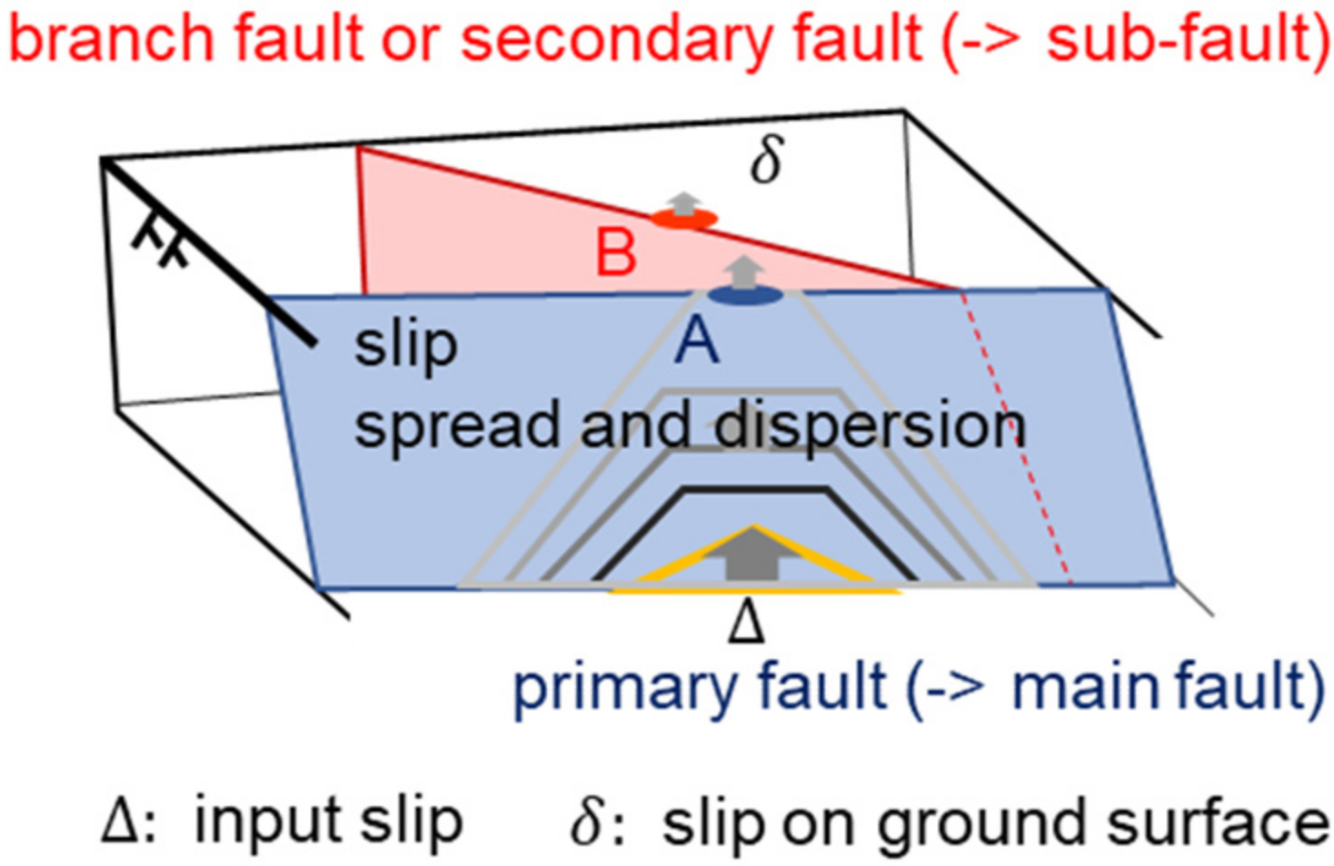
For fault displacement simulations, we constructed a continuum model of the ground and faults (Figure 1). An input slip $\Delta$ was defined at the bottom of the primary (or main) fault and the surface slip $\delta$ was obtained after calculating the spread and dispersion of the slip on the fault plane. For on-site fault assessment at NPPs, the surface slip on branch or secondary faults (or sub-faults) must be estimated, rather than the slip on the main fault.

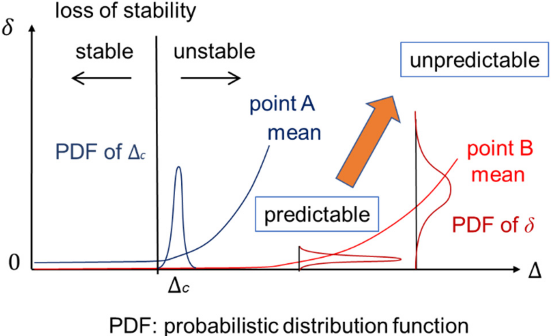
A fundamental difficulty in simulating the fault rupture process is the stability loss in the solutions of the initial and boundary value problems, which leads to significant changes in the solution as a result of small disturbances.

The treatment of uncertainties stemming from limitations in the quality and quantity of available relevant data for underground structures, stress states, and source fault dynamics is important. Numerous simulations must be conducted under different conditions (capacity computing).

When significant uncertainty exists, the surface fault displacement $\delta$ calculated using capacity computing is distributed over a wide range. In this case, $\delta$ was unpredictable. It is important to evaluate the critical input slip ${\Delta }_c$, which is the minimum input slip that causes a surface slip, before evaluating $\delta$. This concept is illustrated in Figure 2.

Quasi-static simulations facilitate the determination of the relationship between the input and surface slips. This is extremely important for the estimation of ${\Delta }_c$. Sawada et al. [13] demonstrated that the calculated ${\Delta }_c$ and $\delta$ from quasi-static simulations were close to those calculated using dynamic simulations with damping and proposed the use of quasi-static simulations for capacity computing. Therefore, quasi-static simulations were adopted in this study. Therefore, the symplectic time integration described above was not used and seismic waves were not included in the simulations.

2.2. FEM for the Fault Displacement Problem

We implemented a rigorous joint element for modeling the slip behavior of faults and a symplectic time integration method with a Hamiltonian formulation using the open-source FEM software FrontISTR [16] to develop a numerical tool for fault displacement simulation [17].

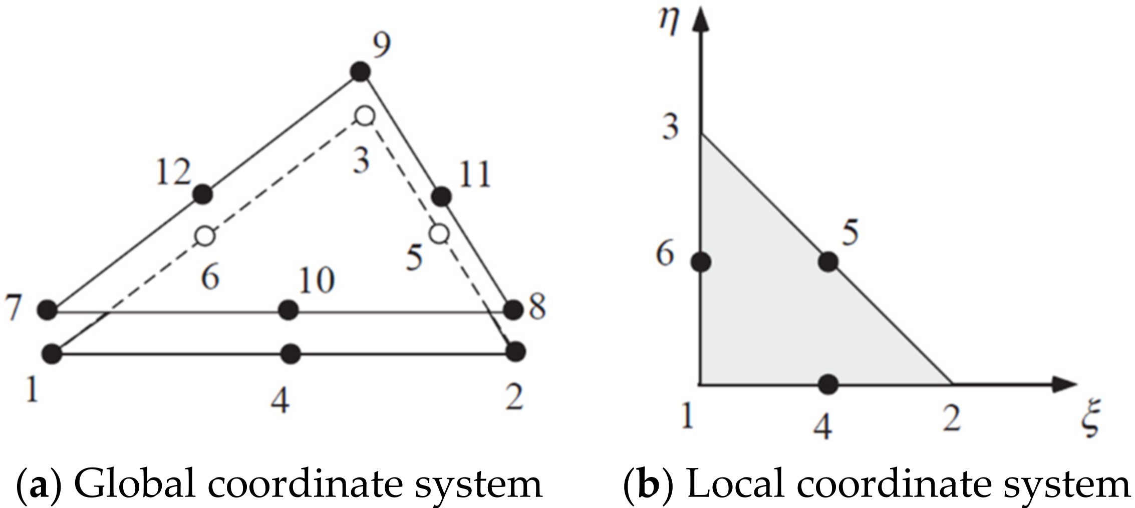
In joint elements that are widely used in the field of rock mechanics, nodal forces are directly calculated from relative nodal displacements on a discontinuity [18]. By using this method, element stiffness matrices can be easily calculated. However, they differ from the standard method for constructing finite elements. Joint elements for fault displacement simulations should be defined to ensure proper convergence for the chosen element sizes and applicability to curved faults. We developed a rigorous joint element in which element stiffness matrices are derived from the Lagrangian on a discontinuous surface using an isoparametric formulation [12]. The following is a formulation for a second-order triangular joint element.

The variant of the Lagrangian $\mathsf{\delta }{L}_J$ is given by the following area integral on the discontinuous surface $S$:

$$\mathsf{\delta }{L}_J=-\int \mathsf{\delta }\mathit{u}\left(2k_n\mathit{n}\otimes \mathit{n}+2k_t\mathit{t}\otimes \mathit{t}\right)\mathit{u}dS,$$

(1)

where $\mathit{u}\left(={\mathit{u}}_{+}-{\mathit{u}}_{-}\right)$ is the relative displacement; ${\mathit{u}}_{+}$ and ${\mathit{u}}_{-}$ are the displacements on the top and bottom surfaces of $S$, respectively; $\mathit{n}$ is the unit normal vector of $S$; $\mathit{t}$ is the unit tangential vector of $S$; and $k_n$ and $k_t$ are the normal and tangential spring constants, respectively. $\mathit{A}\otimes \mathit{B}$ denotes the tensor product of vectors $\mathit{A}$ and $\mathit{B}$.

Considering the case that $S$ is a curved surface, an isoparametric formulation is adopted. The three-dimensional global coordinate system $\mathit{x}$ of $S$ is given by the following function of the two-dimensional local coordinate system $\mathbf{\xi }$ (see Figure 3):

$$\mathit{x}\left(\mathbf{\xi }\right)={{\displaystyle \sum }}_{a=1}^6{N}^a\left(\mathbf{\xi }\right)x^a,$$

(2)

where ${\mathit{x}}^a\left(a=1,2,\dots ,6\right)$ is the nodal coordinate of the joint element and $N^a$ is the shape function. The area integral on $S$ is transformed into the area integral using $\mathbf{\xi }$, and the Gaussian integral is applied:

The unit normal vector $\mathit{n}$ is formulated as follows:

$$\mathit{n}=s_{\mathsf{\xi }}\times s_{\mathsf{\eta }}/\left|s_{\mathsf{\xi }}\times s_{\mathsf{\eta }}\right|,$$

(3)

where $\mathit{A}\times \mathit{B}$ denotes the vector product of vectors $\mathit{A}$ and $\mathit{B}$. The differential global coordinates $\mathit{s}$ is defined as follows:

$$s_{\mathsf{\xi }}=\partial \mathit{x}/\partial \xi , s_{\mathsf{\eta }}=\partial \mathit{x}/\partial \eta .$$

(4)

The unit vectors have the following relationship:

$$\mathit{t}\otimes \mathit{t}=\mathit{e}-\mathit{n}\otimes \mathit{n},$$

(5)

where $\mathit{e}$ is the identity matrix. The element stiffness matrix ${\mathit{E}}_J^{ab}$ is obtained as follows:

$${\mathit{E}}_J^{ab}=\int 2N^a\left(k_n\mathit{n}\otimes \mathit{n}+k_t\mathit{t}\otimes \mathit{t}\right)N^b\left|s_{\mathsf{\xi }}\times s_{\mathsf{\eta }}\right|d\mathsf{\xi }d\eta ,$$

(6)

We implemented joint elements using a nonlinear spring-type constitutive equation to represent fault movement [12,13]. The constitutive equation for the shear movement of the joint element is defined as follows (see Figure 4):

$$\tau =\kappa u,$$

(7)

where $\tau$ is the shear stress and $u$ is the slip on the fault plane. The spring coefficient per unit area (shear stiffness) $\kappa$ is described by the following function for a slip $u$:

$$\kappa \left(u\right)=\left\{\begin{array}{cc}{\kappa }_0-\frac{{\kappa }_0-{\kappa }_d}{u_{cr}}u& \left(u\le u_{cr}\right)\\ {\kappa }_d& \left(u>u_{cr}\right)\end{array}\right.,$$

(8)

where ${\kappa }_0$ is the initial shear stiffness, ${\kappa }_d$ is the final shear stiffness, and $u_{cr}$ is the critical slip. We considered the effects of the normal stress on the shear stiffness of the faults and defined the following equation:

$${\kappa }_0={\tilde{\kappa }}_0\left({\sigma }_n+b\right),$$

(9)

where ${\tilde{\kappa }}_0$ is the shear stiffness per unit of normal stress, ${\sigma }_n$ is the normal stress on the fault plane, and $b$ is a constant. We assumed that the first peak of the slip–shear stress relationship shown in Figure 4 is identical to the shear strength. The parameters ${\kappa }_0$ and $b$ in Equation (9) can be determined such that the shear strength satisfies Coulomb’s law of friction as follows:

$${\tilde{\kappa }}_0=\frac{4\left(1-{\kappa }_d/{\kappa }_0\right)}{u_{cr}}\tan \varphi ,$$

(10)

$$b=\frac{4c}{{\tilde{\kappa }}_0{u}_{cr}}\left(1-{\kappa }_d/{\kappa }_0\right),$$

(11)

where $c$ is the cohesion and $\varphi$ is the friction angle.

3. Simulation

3.1. The 2016 Kumamoto Earthquake

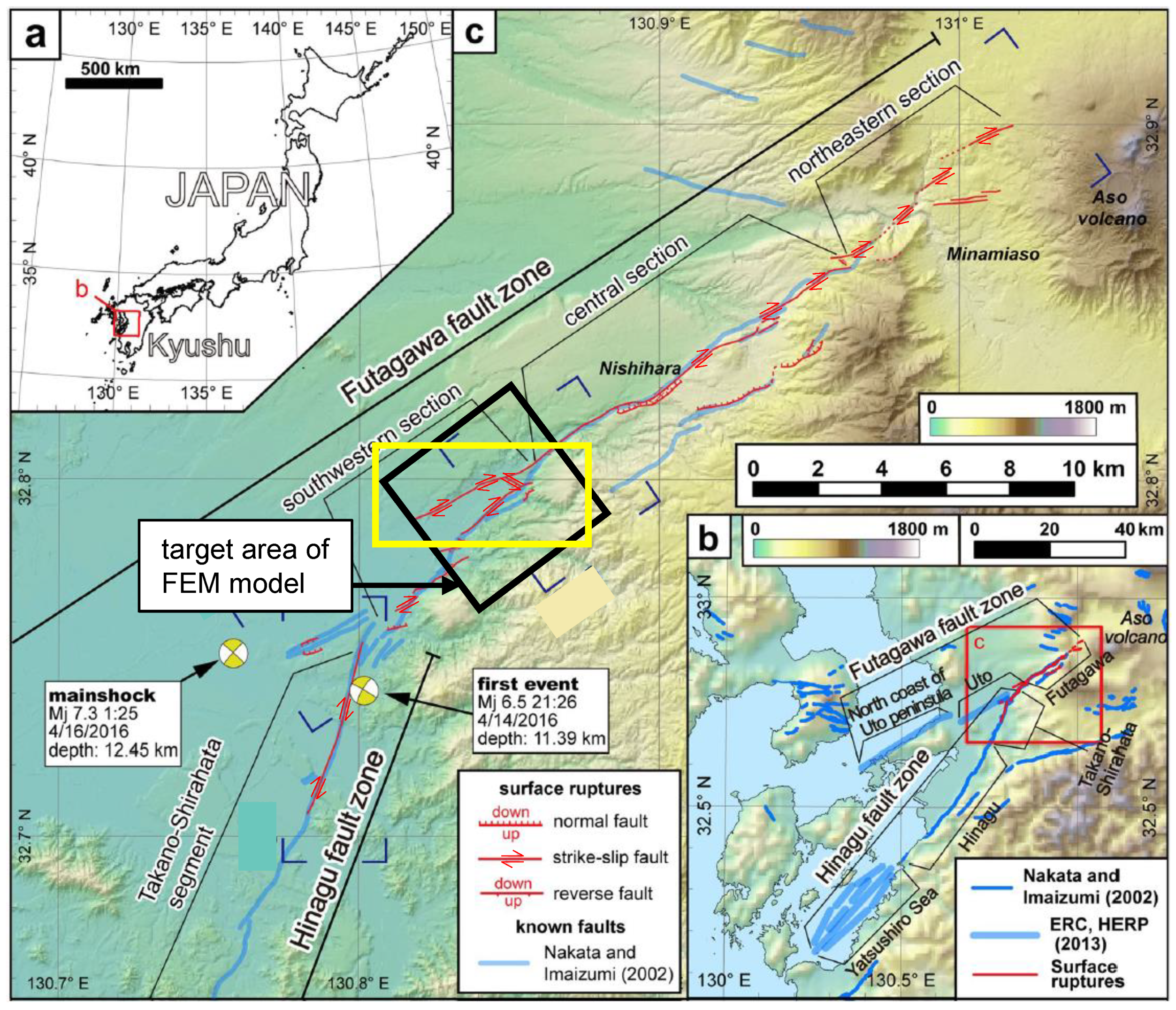
The 2016 Kumamoto earthquake began with a Japan Meteorological Agency magnitude (M_JMA) 6.5 earthquake in Kumamoto Prefecture in the central part of Kyushu Island in southwest Japan at 21:26 Japan Standard Time (JST) on 14 April 2016. A larger M_JMA 7.3 earthquake occurred at 01:25 JST on 16 April 2016, just 28 h later. A seismic intensity observation station at the Mashiki town hall recorded a seismic intensity of seven on the JMA scale during both events. The M_JMA 6.5 event on 14 April was the foreshock and the M_JMA 7.3 event on April 16 was the mainshock. The mainshock was the simulation target considered in this study.

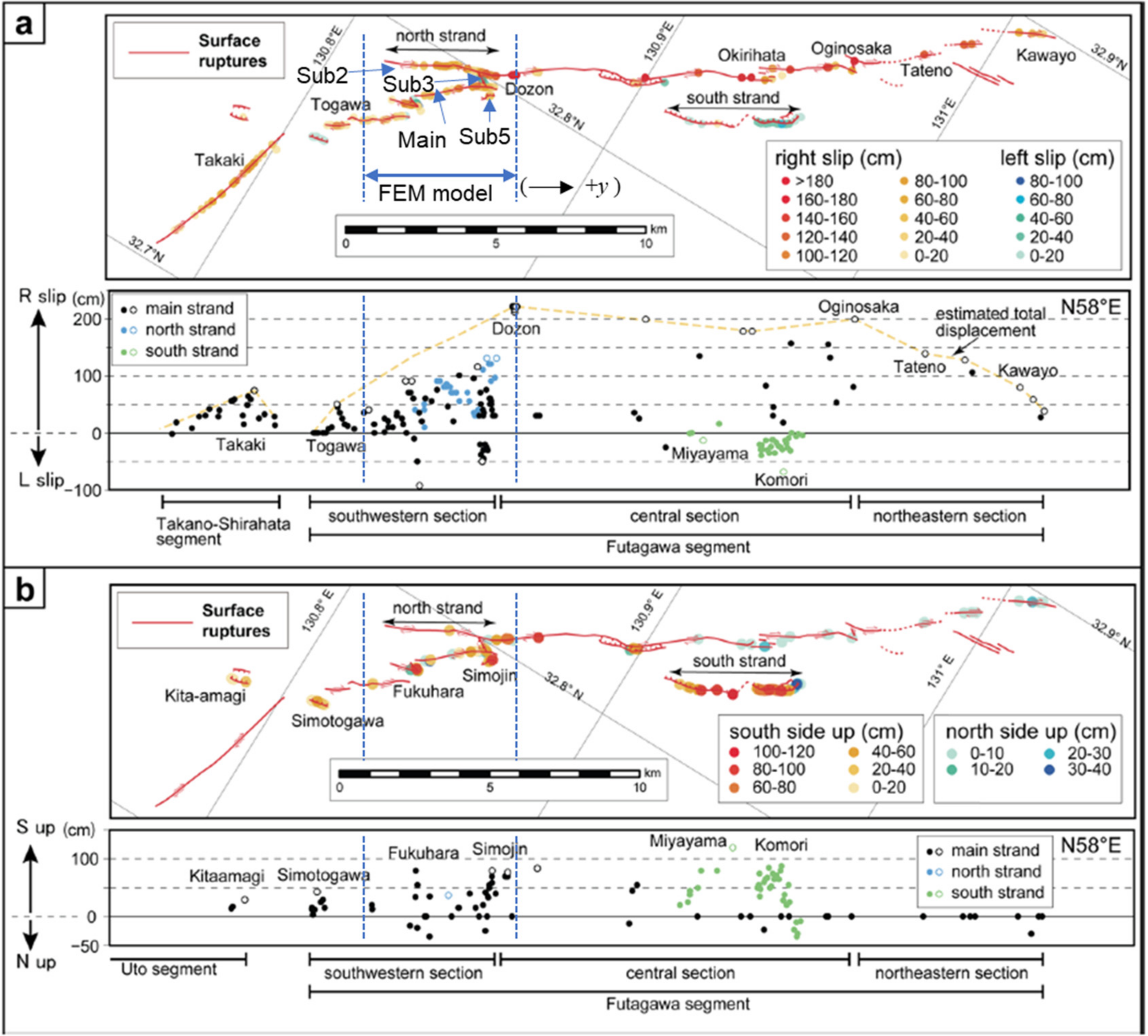
The earthquake occurred along the Futagawa and northern Hinagu fault zones [19]. Surface faults of 28 and 6 km in length were observed along the Futagawa and Hinagu fault zones, respectively (see Figure 5). Vertically, the north side of the Futagawa fault zone sank ≥1.0 m and the south side rose ≥0.3 m. Horizontally, the north side was displaced by more than 1.0 m to the east and the south side was displaced by more than 0.5 m to the west. The surface faults were investigated and the fault displacement distribution along the faults was obtained [20]. A right-lateral strike-slip fault of up to 2.2 m was observed at Dozon in the eastern part of Mashiki. The surface fault branched into two faults from Dozon to the west. Although these two branched-out faults exhibited a right-lateral strike-slip fault, a left-lateral strike-slip fault was observed between them. The target area of our numerical simulations was a 5 × 5 km square area containing the faults around Dozon, as shown in Figure 5.

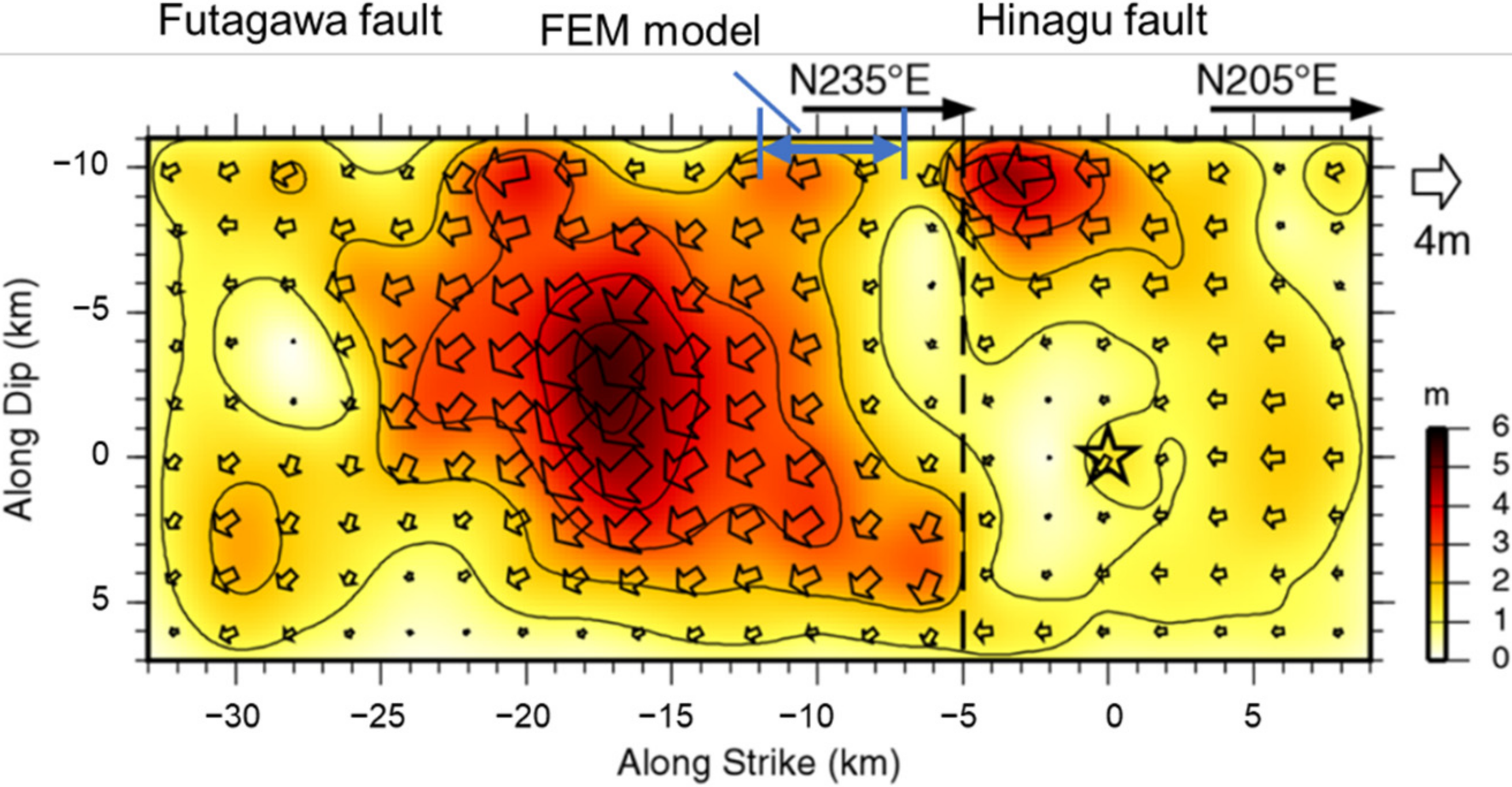
Asano and Iwata [21] conducted a seismic source inversion analysis of the 2016 Kumamoto earthquake and obtained the slip distributions on the Futagawa and Hinagu faults (Figure 6). The Futagawa and Hinagu faults slipped in the form of right-lateral strike-slip faults, including a normal fault component. The slip near the target area of the simulation ranged from 1.7 to 2.6 m.

3.2. Analytical Model

The target of our simulations was a 5 × 5 km square area containing the branched-out faults in Mashiki town. The target depth from the ground surface was approximately 1 km. The National Research Institute for Earth Science and Disaster Resilience provides a database of the crustal structure density and elastic wave velocity covering all of Japan on the website of the Japan Seismic Hazard Information Station (J-SHIS) [22]. In this database, elevation data regarding the ground surface and boundaries of elastic wave velocity and density are provided at the center of every grid of 30 arcseconds of latitude and 45 arcseconds of longitude. By using this database, we constructed an analytical model that includes the shape of the land and crustal structure. We determined the strike and dip angles of the Futagawa and Hinagu faults by referring to the paper by Asano and Iwata [21]. The dip angles of the Futagawa and Hinagu faults were 65° N and 72° N, respectively. Although the upper edges of the faults did not reach the ground surface, we extended them to the ground surface with the same dip angle.

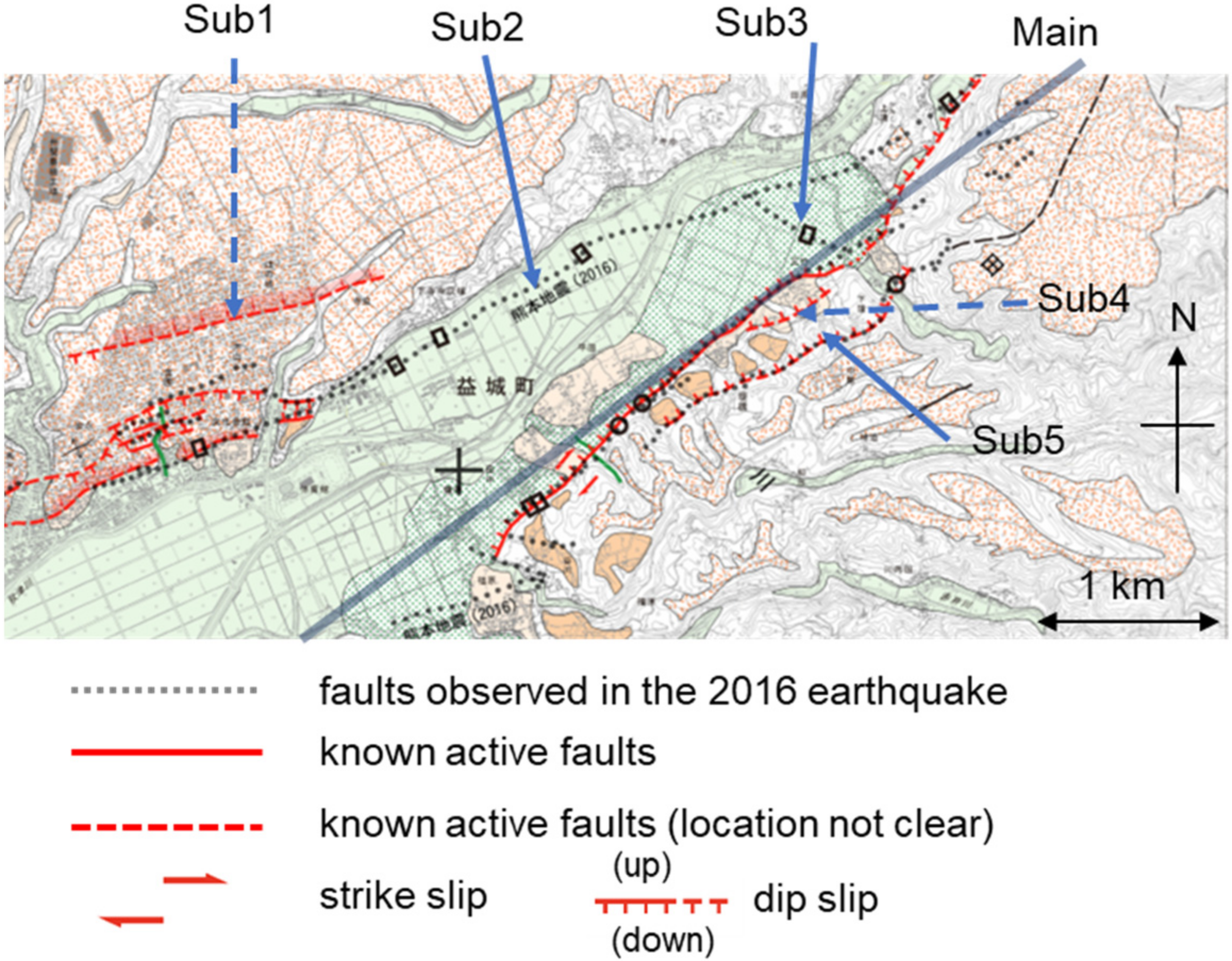
Figure 7 presents the surface faults along the Kiyama river in Mashiki town, where the Futagawa fault branches out into 2 faults. We treated the line labeled “Main”, which is one of the two branched-out faults, as the main fault, which is identical to the Futagawa fault. The other faults, which are labeled as “SubN”, were included in the analytical model as sub-faults. Three faults, namely Sub2, Sub3, and Sub5, were observed during the 2016 earthquake, with Sub2 being the other branched-out fault. Sub3 was a left-lateral strike-slip fault bridging the main fault and Sub2. Sub1 and Sub4 were faults known to exist before the 2016 earthquake. However, surface faulting was not observed along them during the earthquake.

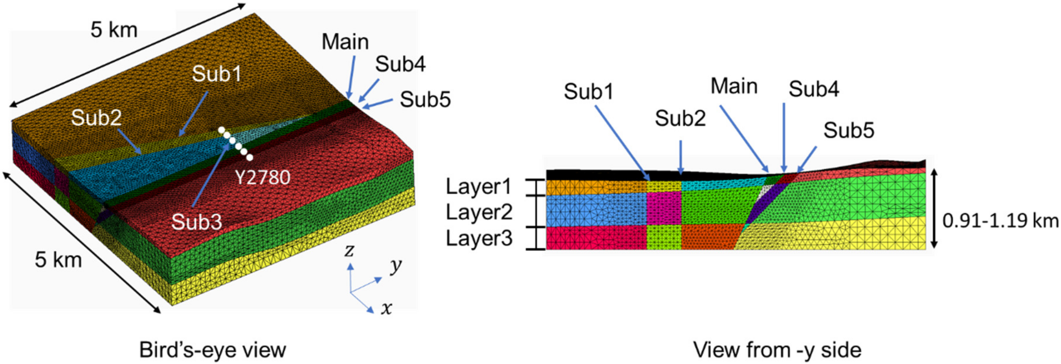
Figure 8 presents the finite element mesh of the analytical model. Faults are extended to the outer boundary or to other faults. The main fault, Sub4, and Sub5 strikes are parallel to the y axis. The sub-fault dip angles were determined based on the results of a seismic reflection survey by Aoyagi [23]. Sub1, Sub2, and Sub4 are vertical. The ground is divided into three layers based on the J-SHIS database. The ground is discretized using second-order tetrahedral elements and the fault planes are discretized using second-order triangular joint elements. The fault plane element size is approximately 50 m and the total number of degrees of freedom is approximately 3.76 million. The white dots from a bird’s-eye view in Figure 8 indicate the locations of the output points for the fault displacement results. “Y2780” indicates that the y coordinate of these plots is 2780 m.

We assumed that the ground was a linear elastic body and derived the Young’s modulus and Poisson’s ratio of each layer from the density and elastic wave velocity values in the J-SHIS database. We conducted an initial stress analysis to determine the values of the parameters ${\tilde{\kappa }}_0$ and $b$ on the fault planes using Equations (10) and (11) before fault displacement analysis. Normal displacements were fixed at the bottom and side boundaries in the initial stress analysis. We assumed a cohesion of 0.025 MPa and friction angle of 25° on the fault planes by reference to the experimental value of the crushed zone in NPP sites [14]. The ratio between the initial and final shear stiffness ${\kappa }_{\mathrm{d}}/{\kappa }_0$ was assumed to be 0.01 in reference to the analyses conducted using a simple ground/fault model and a real earthquake ground model [13,14]. The critical slip $u_{cr}$ was 0.1 m in reference to the value used in the dynamic rupture simulation of the fault [4]. The material parameter values are summarized in

Table 1. Material parameters.

	Young’s Modulus (GPa)		Poisson’s Ratio	Density (g/cm3)
Layer1	7.18		0.38	2.15
Layer2	27.7		0.31	2.40
Layer3	63.3		0.27	2.60
	friction angle (deg)	cohesion (MPa)	shear stiffness ratio ${\kappa }_d/{\kappa }_0$	critical slip (m)
faults	25	0.025	0.01	0.1

.

The size of the analytical model is presented in Figure 8 and is smaller than the length of the main fault. The boundary conditions of the analytical model were determined using large-scale analysis. We used the elastic theory of dislocations [2] with a slip distribution on the main faults, as shown in Figure 6, as the input. The upper edge of the fault is at a depth of 2 km. We extended the faults to the ground surface and assumed that the slip on the extension was the same as that just below the extension. The ground displacement was calculated and the forced displacement at the bottom of the FEM model was determined. The maximum slip on the bottom of the main fault was 5.2 m, which is twice the estimated 2.6 m slip. The other outer model boundaries were traction free. We refer to this simulation as case1.

3.3. Results

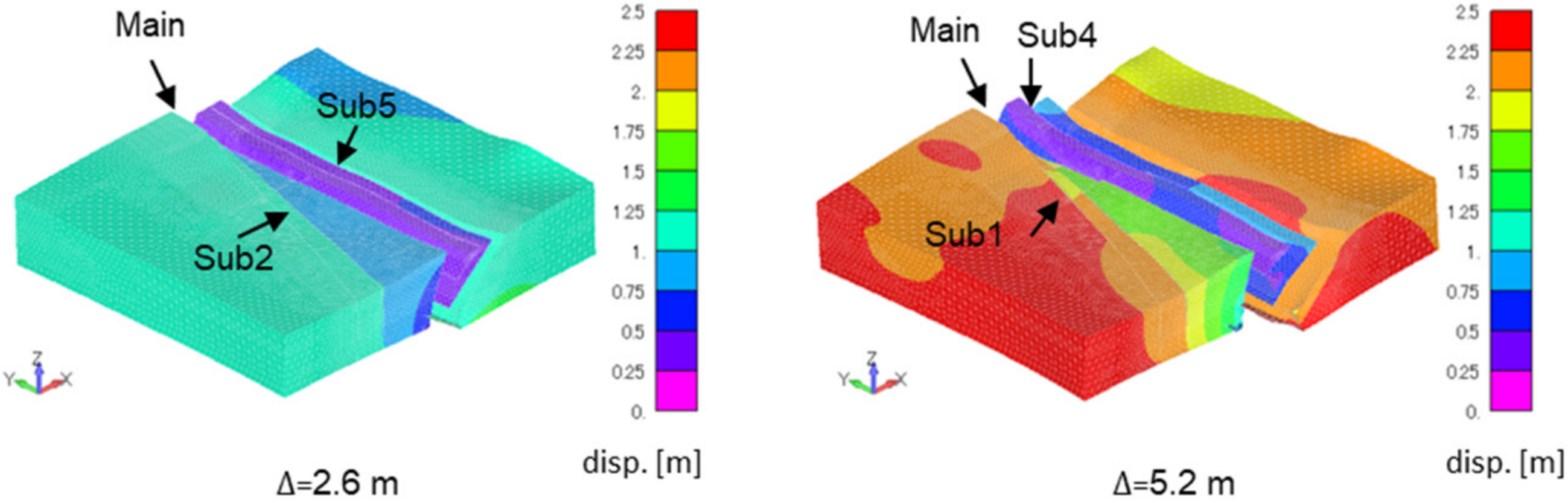
Figure 9 presents the displacement magnitude contour and deformation of the analytical domain. The deformation is presented with 300-times amplification. When $\Delta$ is 2.6 m, which is the slip estimated by Asano and Iwata [21], there is a displacement gap along the main fault, Sub2, and Sub5. Additionally, there is a displacement gap along Sub1 and Sub4 when $\Delta$ is 5.2 m, which is twice the estimated slip value. This gap indicates a surface slip on each fault.

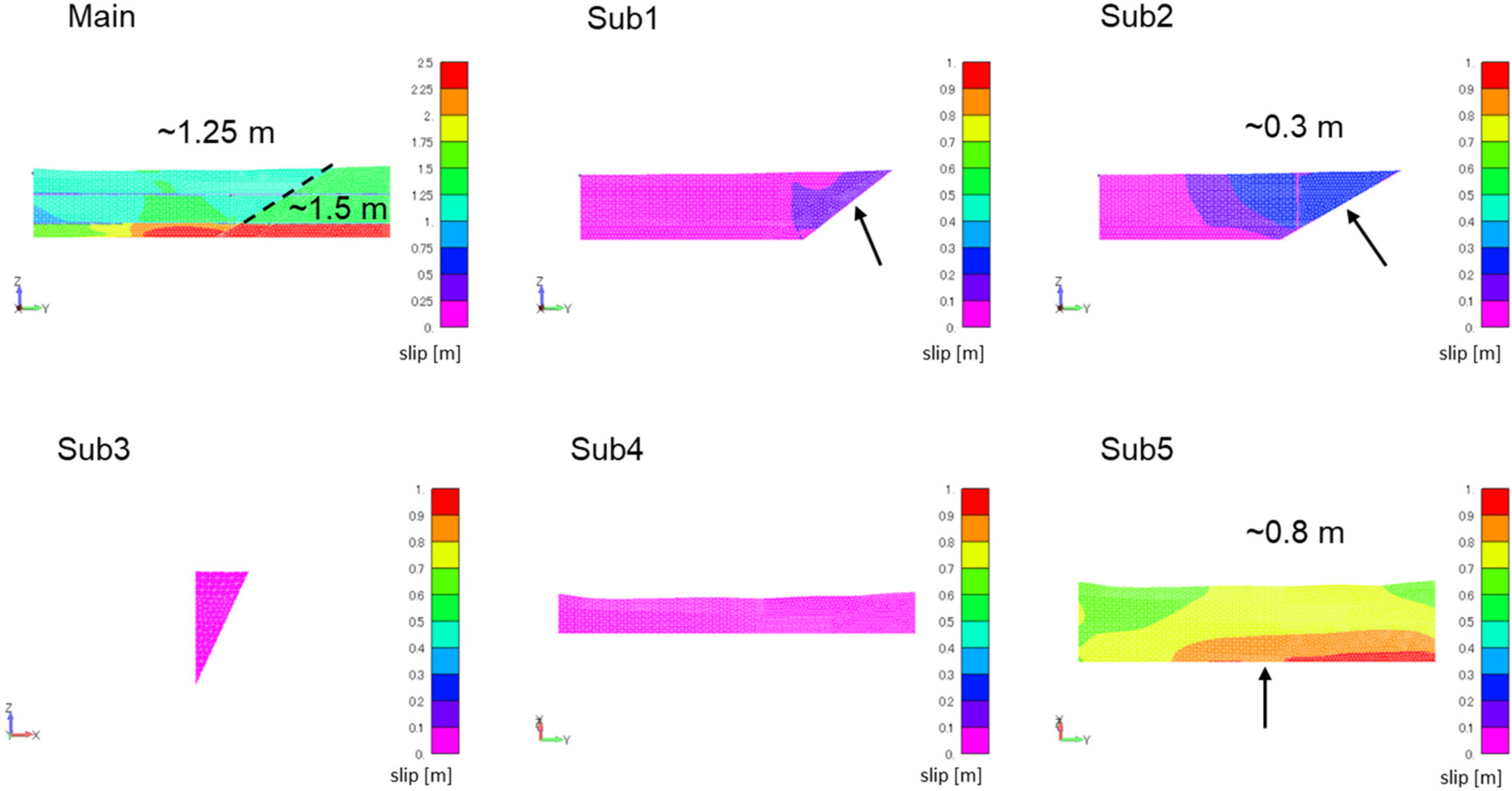
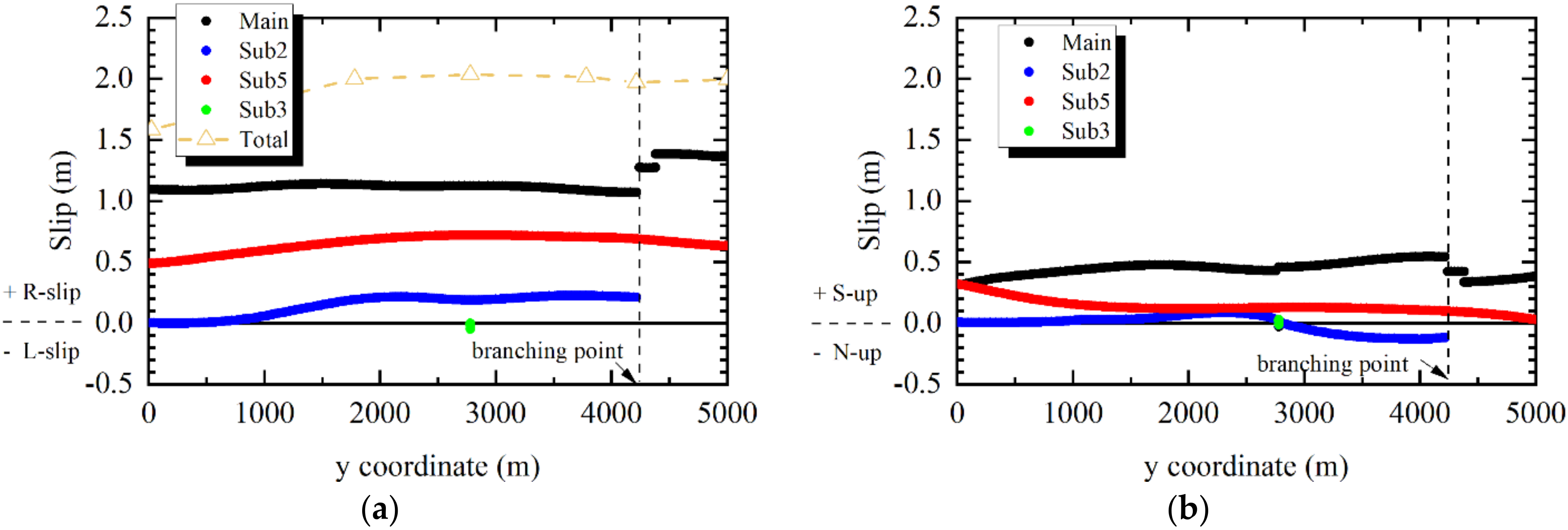
Figure 10 presents contour slip plots at $\Delta =2.6$ m on the main and sub-faults. There is a surface slip of greater than 1.0 m on the main fault and surface slips of greater than 0.1 m on Sub1, Sub2, and Sub5. The slipped area on Sub1 is limited compared to those on Sub2 and Sub5. The surface slips on the main, Sub2, and Sub5 faults are up to 1.25, 0.3, and 0.8 m, respectively. Figure 11 presents the profiles of the surface slip for the strike-slip and vertical components along Main, Sub2, Sub3, and Sub5. Figure 12 presents the observed slip distributions along the Futagawa fault and Hinagu fault [20]. Comparing the calculated and observed strike-slip, the calculated slip is smaller on Sub2. On the other hand, the surface slip on Sub5 distributes in a longer section in the calculation. The sum of the calculated surface strike-slip values (approximately 2.0 m) is in good agreement with the total displacement of the southwestern section of the Futagawa segment in Figure 11. The vertical component of the calculated surface slip on the main fault is intermediate to the observed ones, but the sum of the vertical slips on the main fault and Sub5 mostly exceeds the observed ones.

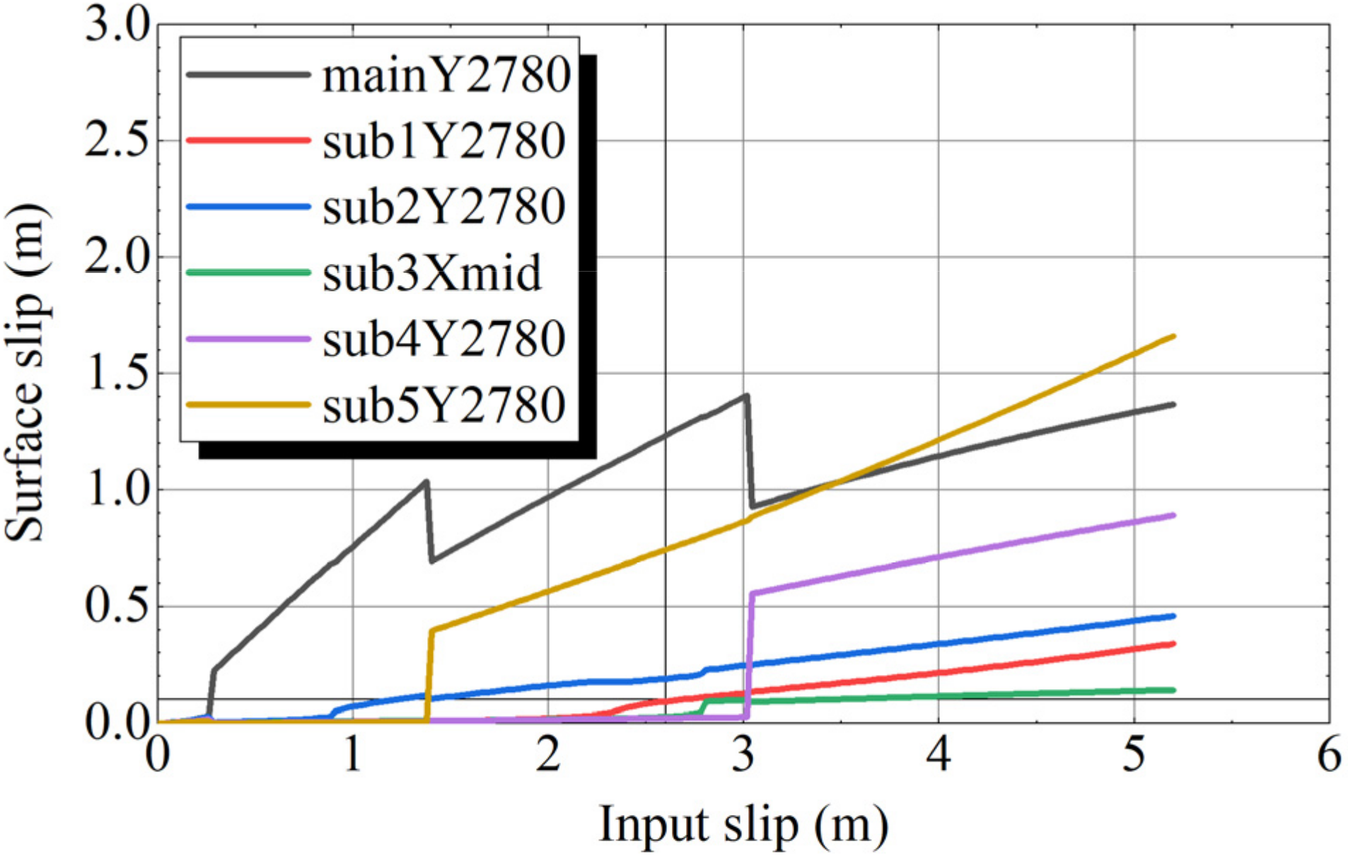
Figure 13 presents the variation in the surface net slip $\delta$ as the input slip $\Delta$ increases. There is a steep increase in the surface slip at $\Delta =0.29$ m on the main fault. A steep increase in the surface slip on Sub5 and Sub4 begins at $\Delta =1.40$ m and $\Delta =3.04$ m, respectively. Although there is no steep increase on Sub2, Sub1, or Sub3, the slips are greater than 0.1 m at $\Delta =1.22$ m, $\Delta =2.68$ m, and $\Delta =3.02$ m, respectively. We define ${\Delta }_c$ as the input slip at which the surface slip exceeds 0.1 m and summarize the values of ${\Delta }_c$ at 3 locations on each fault in

Table 2. Slip sense and ${\Delta }_c$ on each fault (case1).

Fault	Location *	Observation	${\mathbf{\Delta }}_{\mathit{c}}\left(\mathbf{m}\right)$	Simulation
Main	1	right-lateral	0.29	right-lateral	east-up
	2		0.29	right-lateral	east-up
	3		0.29	right-lateral	east-up
Sub1	1	-	-	-	-
	2		2.68	right-lateral	east-up
	3		2.44	right-lateral	east-up
Sub2	1	right-lateral	1.69	right-lateral	east-up
	2		1.22	right-lateral	west-up
	3		0.91	right-lateral	west-up
Sub3	1	left-lateral south-up	4.32	-	south-up
	2		3.06	left-lateral	south-up
	3		2.83	left-lateral	south-up
Sub4	1	-	3.04	right-lateral	east-up
	2		3.04	right-lateral	east-up
	3		3.04	right-lateral	east-up
Sub5	1	east-up	1.40	right-lateral	east-up
	2		1.40	right-lateral	east-up
	3		1.40	right-lateral	east-up

* Locations 1, 2, and 3 indicate the positions of the minimum, medium, and maximum × coordinates on Sub3 and the positions of 1780, 2780, and 3780 m in the y coordinates on the other faults, respectively.

. ${\Delta }_c$ is small for Sub2 and Sub5, where the surface displacement was actually observed in the 2016 earthquake. The sense of the slip at each location is presented in Table 2. The sense of the slip in the simulations was remarkably similar to that of the observed surface faults, as shown in Figure 12.

3.4. Discussion

We constructed a 5 × 5 × 1 km analytical model and derived the boundary conditions from the elastic theory of dislocation using a slip distribution in the main fault obtained from seismic source inversion analysis. When forced slip occurred at the bottom of the main fault, we observed a steep increase in the surface slip on the main and sub-faults. On the sub-faults that appeared in the 2016 earthquake, the surface slip appeared at a smaller input slip than on the other sub-faults. The sense of slip on each fault in our simulations was remarkably similar to the observations during the real earthquake.

As shown in Figure 12, the surface fault slip is distributed in an uneven manner. Although there are locations where significant slip occurs, there are many locations where the slip is small or does not occur in the entire section. The calculated surface slip distribution is continuous and agrees well with the measured total slip distribution (enveloped slip distribution curve). This indicates that the proposed numerical method enables a conservative estimation of surface fault slip.

The arrows in Figure 10 represent the Sub1, Sub2, and Sub5 contact edges with the main fault. The slipped sub-fault areas propagate from these contact edges. In the 2014 Nagano-ken-hokubu earthquake simulation [14], the slip on the sub-fault was larger near the surface than near the contact edge with the main fault. The slip distribution on the sub-faults was remarkably different between the two earthquake simulations.

However, some phenomena were not reproduced in our simulations. For example, the surface slip on Sub3 requires a large input slip. In the simulations, the small faults tended to be less likely to slip.

In general, faults are identified from ruptures left on the ground surface. It is difficult to include faults that cannot be identified from the ground surface in the model. Moreover, it is difficult to fully capture the subsurface structure and connectivity of faults. In the analysis of this paper, faults were extended to the model boundaries or other faults. The larger the fault plane, the greater the possibility that large displacements will be calculated. On the other hand, if many faults are identified, it is difficult to represent all of them with joint elements. As sub-faults, it is reasonable to include in the model faults that are relatively large or that affect the focused facilities. In general, if the number of faults is limited rather than considering many faults, the fault displacement for each single fault will be calculated as larger. However, this needs to be further investigated.

4. Predictive Simulation

4.1. Setting of Input Conditions

4.1.1. Basic Slip Distribution on Primary Faults

For predictive simulation, we were not able to use the results from the seismic source inversion analyses shown in Figure 6 and we had to assume the slip distribution on the main fault. In this paper, we propose a method to set the slip distribution on the main fault and apply it to predictive simulation using an analysis model of the 2016 Kumamoto earthquake. We ignore the Hinagu fault and consider a scenario in which only the Futagawa fault ruptures in the following predictive simulations.

We set the slip distribution using a strong motion prediction method called recipe [24], which includes the following steps: (1) set the main fault geometry (length, width, depth, and dip angle), (2) calculate the seismic moment, (3) calculate the average slip from the seismic moment and shear modulus of the crust, and (4) set the asperity number and location to calculate the slip on them and on the background. To calculate the seismic moment $M_0$, the following equation is used for relatively large earthquakes [25]:

$$M_0={\left(\frac{S}{4.24}\times {10}^{11}\right)}^2\times {10}^{-7},$$

(12)

where $S$ denotes the square of the main fault. We adopted the geometry of the Futagawa Fault presented by Asano and Iwata [21]. Because $S=5.04\times {10}^8$ m² was derived from a length of 28 km and width of 18 km, $M_0$ was calculated as $1.41\times {10}^{19}$ Nm. The average slip $D$ was calculated from $S$ and the shear modulus $\mu$ using the following equation:

$$D=M_0/\left(\mu \cdot S\right).$$

(13)

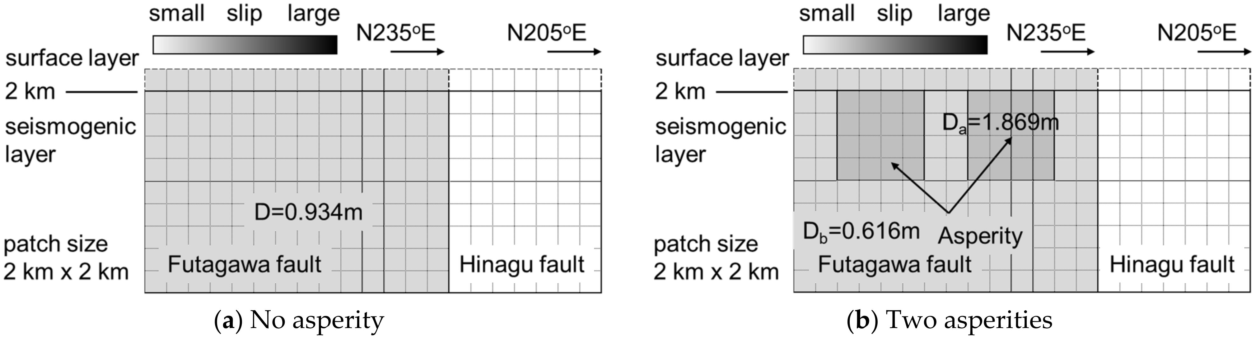
when we used $\mu =30$ GPa, which was based on the assumption of a hard rock mass in the deep underground, $D=0.934$ m was obtained. We set a uniform slip distribution of 0.934 m on the entire Futagawa fault, as shown in Figure 14a, and conducted our first predictive simulation. We refer to this simulation as case2.

In this recipe, asperities were set on the seismic source fault. Subsequently, we set the slip distribution by considering the existence of asperities. Although it is recommended to use an empirical equation for the relationship between the short-period level and equivalent radius of the total asperity area, we determined the total asperity area to be $1.28\times {10}^8$ m² by referring to research on the ratio of the total asperity area to the total fault area introduced in the recipe. We placed 2 asperities of equal area (64 km²) on the Futagawa fault, as shown in Figure 14b. The average slip of asperity $D_a$ was determined to be $\xi$ times the average slip $D$ as:

$$D_a=\xi D,$$

(14)

where $\xi =2$ was used based on an analysis of recent crustal earthquakes. The average slip of the background $D_b$ was derived from the following equations:

$$M_{0a}=\mu D_a{S}_a,$$

(15)

$$M_{0b}=M_0-M_{0a},$$

(16)

$$D_b=M_{0b}/\left(\mu \cdot S_b\right),$$

(17)

where $M_{0a}$ is the total seismic moment of the asperities, $S_a$ is the total area of the asperities, $M_{0b}$ is the seismic moment of the background, and $S_b$ is the area of the background. We obtained $D_a=1.869$ m and $D_b=0.616$ m. We set these slip values on the Futagawa fault, as shown in Figure 14b, and conducted a second predictive simulation. We refer to this simulation as case3.

4.1.2. Large Surface Slip Area

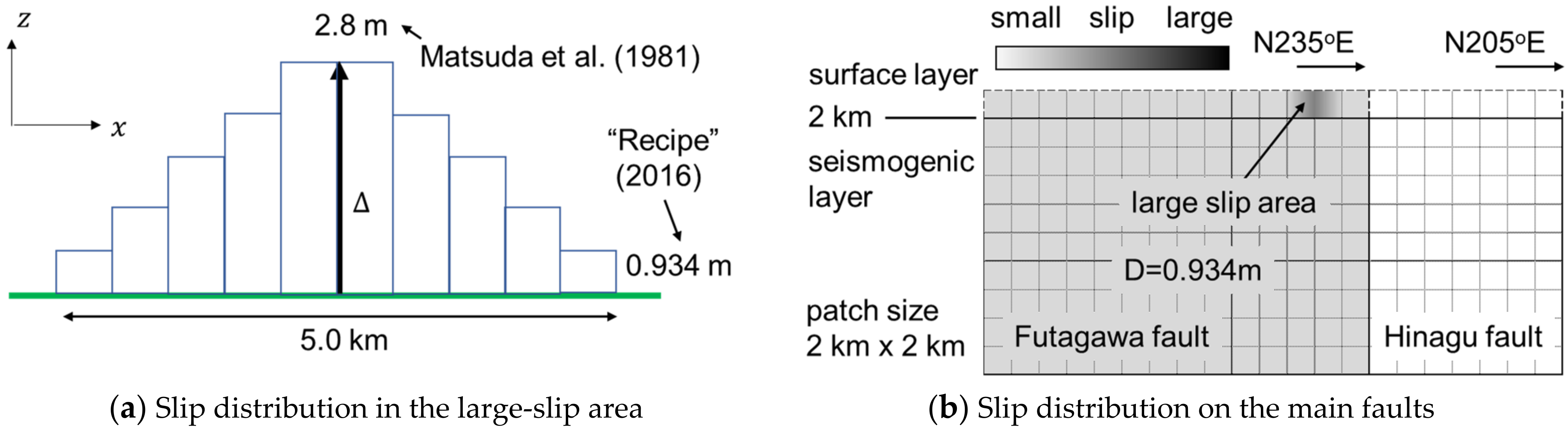
When we set the slip distribution on the main fault based on the recipe, the surface slip was uniform and smaller than that observed during the 2016 Kumamoto earthquake. The slip along the surface fault was not generally uniform. Therefore, we set a large slip area on the main fault based on case2, as shown in Figure 15. The following empirically obtained equation proposed by Matsuda et al. [26] was used to set the maximum surface slip:

$$D_{\max }={10}^{-4}L,$$

(18)

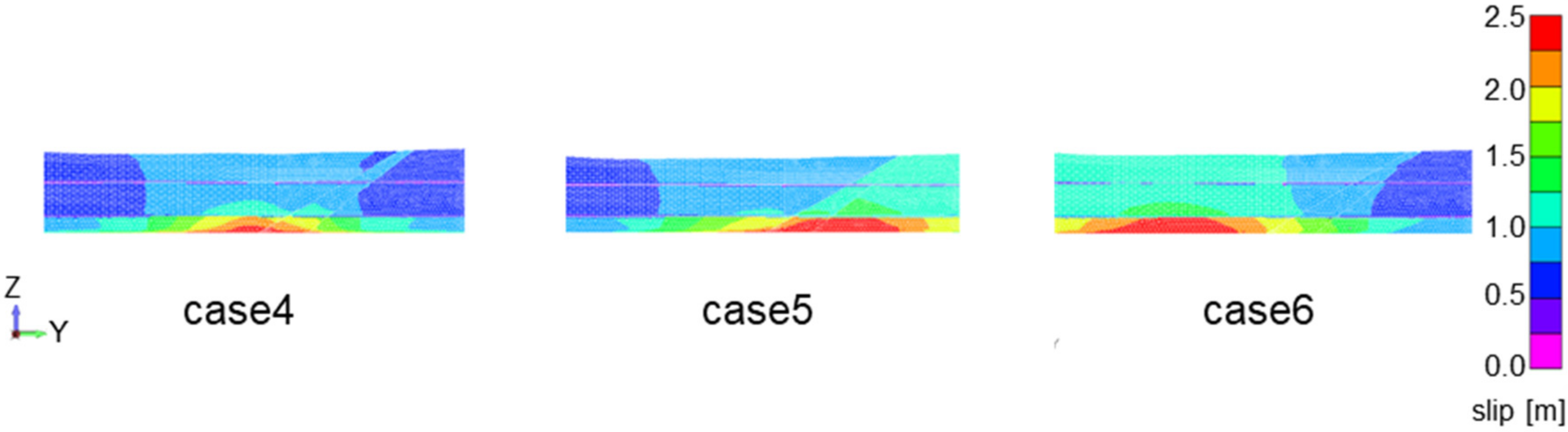
where $D_{\max }$ is the maximum surface slip and $L$ is the surface rupture length. Here, we used the 28 km fault length for $L$ and obtained $D_{\max }=2.8$ m. Other equations have been proposed to relate surface fault displacement to the length of faults [27]. We can also use these equations. We assumed that the length of the large surface slip area was 5 km, which is the same as the size of the FEM model, and that the peak slip position was identical to the center of the FEM model. We refer to this simulation as case4.

Additionally, we set up 2 cases in which the large surface area was shifted by +1 km and −1 km in the y direction compared to case4, which are referred to as case5 and case6, respectively.

In simulations case2 to case6, the maximum forced slip at the bottom of the FEM model was twice that of the slip distribution.

4.2. Results

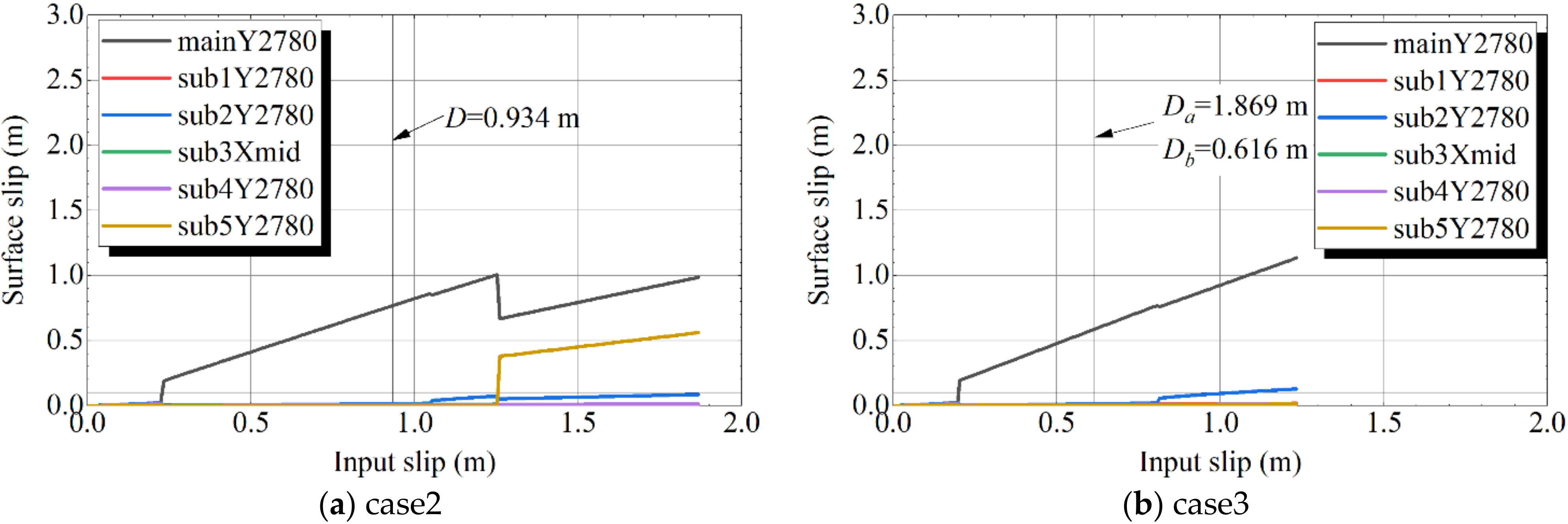
Figure 16 presents the variation in the surface net slip $\delta$ in case2 and case3 as the input slip $\Delta$ increases. In case2, there is a steep increase in the surface slip at $\Delta =0.22$ m on the main fault and only the main fault slips before $\Delta =0.934$ m. The ${\Delta }_c$ value of Sub5 is 1.25 m, which is similar to the value obtained in case1 (1.40 m). In case3, only the main fault slips before twice the value of $D_b$ is inputted, despite the fact that twice the value of $D_a$ was inputted in the asperities.

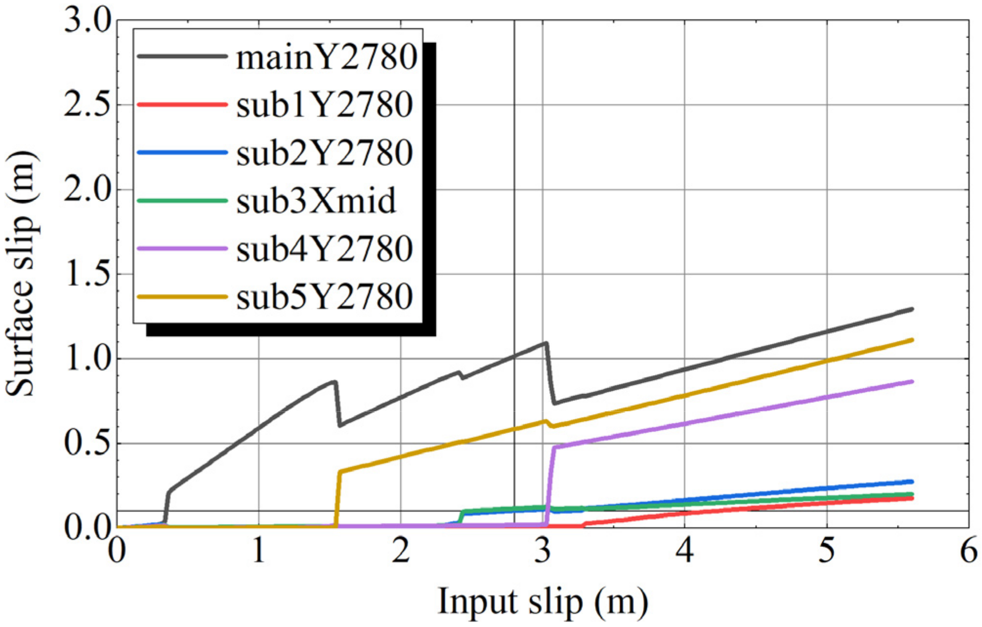
Figure 17 presents the variation in the surface net slip $\delta$ in case4 as the input slip $\Delta$ increases. There is a steep increase in the surface slip at $\Delta =0.36$ m on the main fault. The ${\Delta }_{\mathrm{c}}$ values on Sub1, Sub2, Sub3, Sub4, and Sub5 are 4.2, 2.7, 2.5, 3.1, and 1.6 m, respectively. In Sub2, Sub3, and Sub5, where surface fault displacement can be observed, ${\Delta }_{\mathrm{c}}$ is less than 2.8 m. This tendency is similar to the case1 results. The surface slip is slightly smaller in case4 than in case1. Although the slip distributions at depth are significantly different between case1 and case2, the surface slips on the sub-faults are similar.

Figure 18 presents the variation in the surface net slip $\delta$ on Sub2, Sub3, and Sub5 in case4, case5, and case6 as the input slip $\Delta$ increases. The results for Sub5 are similar between the three cases. However, the ${\Delta }_c$ values on Sub2 and Sub3 are much smaller in case5 than in case4 and case6. As shown in Figure 19, the peak of the large slip area is close to the intersection line between the main fault and Sub2 fault. In contrast, in case6, no surface slip occurs on sub-faults Sub2 and Sub3 because the location of the maximum slip on the main fault is far from the intersection between the main fault and Sub2 fault. These results indicate that the slips on the sub-faults are strongly affected by the slip distribution on the main fault close to the sub-faults.

4.3. Discussion

We propose a method for setting the slip distribution on the main fault for predictive simulations based on the method of constructing characterized source models for the prediction of strong motion. In cases without asperities and with two asperities, surface slip on the sub-faults did not appear. These results suggest that surface displacement is less likely to occur on sub-faults. In the case with two asperities, a large slip was inputted into the asperities, and it had little effect on the surface slip on the sub-faults.

We also set up cases in which a large surface slip area was located near the sub-faults. We adopted an empirical equation for the relationship between the maximum surface displacement and fault length. We then placed the large slip area in a section of the FEM model. From this simulation, we obtained results similar to those of the simulation with the inversely analyzed input slip. The location of this large slip area had a strong effect on the surface slip of the sub-faults. In other words, for surface slip to occur on a sub-fault, a large slip must occur on a nearby main fault. The probability of a large slip being very close to a sub-fault is relatively small and this condition is extreme.

5. Conclusions

We developed a parallel FEM program to estimate surface fault displacement. In this study, we applied a numerical method to simulate the 2016 Kumamoto earthquake, where the seismic source fault ruptured in the form of a right-lateral strike slip fault, including a normal fault component. We modeled a 5 × 5 × 1 km domain, including branched-out faults and other sub-faults in Mashiki town. We applied forced displacements on the bottom surface of the model based on the slip distribution on the main faults and elastic theory of dislocation. As the input slip increased, surface slips appeared on both the main and sub-faults. In the simulations, the surface slip appeared at a smaller input slip on the sub-faults compared to the observed values during the 2016 earthquake. The sense of slip on each fault in the simulations was in good agreement with that observed during the earthquake. Furthermore, the calculated surface slips agreed well with the envelope curve of the measured surface slip distribution. This was the second application of the numerical method to real earthquakes. Because our simulations reproduced the main features of two different earthquakes with reasonable accuracy, the proposed numerical method should be applicable to surface fault displacement estimation.

We also proposed a method for setting a slip distribution on main faults for predictive simulation based on a method for strong motion prediction. However, surface slip did not appear on the sub-faults, even in the case with two asperities. We then set up a large slip area near the sub-faults based on an empirical equation of the relationship between the maximum surface slip and the length of a fault. In this simulation, we obtained results similar to those of the simulation with the inversely analyzed input slip. We consider that the slip distribution on the main fault with a large slip area is an extreme case in which surface slip on the sub-faults is likely to occur.

In this paper, we presented fault displacement evaluation using quasi-static simulation. As a next step, we aim to evaluate the superposition of fault displacement and earthquake ground vibration by dynamic analysis that takes into account the rupture propagation of the fault.

References

- On-Site Fault Assessment Method Review Committee of Japan Nuclear Safety Institute, Assessment Methods for Nuclear Power Plant against Fault Displacement. Available online: http://www.genanshin.jp/archive/sitefault/data/JANSI-FDE-03r1.pdf (accessed on 7 December 2021).
- Okada, Y. Internal deformation due to shear and tensile faults in a half-space. Bull. Seismol. Soc. Am. 1992, 82, 1018–1040. [Google Scholar] [CrossRef]
- Harris, R.; Day, S. Dynamics of fault interaction: Parallel strike-slip faults. J. Geophys. Resear. 2008, 98, 4461–4472. [Google Scholar] [CrossRef]
- Kase, Y.; Kuge, K. Rupture propagation beyond fault discontinuities; significance of fault strike and location. Geophys. J. Int. 2001, 147, 330–342. [Google Scholar] [CrossRef]
- Kame, N.; Rice, J.R.; Dmowska, R. Effects of prestress state and rupture velocity on dynamic fault branching. J. Geophys. Res. 2003, 108, 2265. [Google Scholar] [CrossRef]
- Aagaard, B.T.; Anderson, G.; Hudnut, K.W. Dynamic rupture modeling of the transition from thrust to strike slip motion in the 2002 Denali Fault Earthquake, Alaska. Bull. Seismol. Soc. Am. 2004, 94, S190–S201. [Google Scholar] [CrossRef]
- Dalguer, L.; Irikura, K.; Wu, H. Permanent displacement from surface-rupturing earthquakes: Insights from dynamic rupture of Mw7.6 1999 Chi-chi Earthquake. In Proceedings of the 16th World Conference Earthquake Engineering, Santiago, Chile, 9–13 January 2017. paper-1004. [Google Scholar]
- Dalguer, L.A.; Wu, H.; Matsumoto, Y.; Irikura, K.; Takahama, T.; Tonagi, M. Development of dynamic asperity models to predict surface fault displacement caused by earthquakes. Pure Appl. Geophys. 2019, 177, 1983–2006. [Google Scholar] [CrossRef]
- Bruhat, L.; Klinger, Y.; Vallage, A.; Dunham, E.M. Influence of fault roughness on surface displacement: From numerical simulations to coseismic slip distributions. Geophys. J. Int. 2020, 220, 1857–1877. [Google Scholar] [CrossRef]
- Oglesby, D.D. What can surface-slip distributions tell us about fault connectivity at depth? Bull. Seismol. Soc. Am. 2020, 110, 1025–1036. [Google Scholar] [CrossRef]
- Wang, Y.; Goulet, C. Validation of fault displacements from dynamic rupture simulations against the observations from the 1992 Landers earthquake. Bull. Seismol. Soc. Am. 2021, 111, 2574–2594. [Google Scholar] [CrossRef]
- Sawada, M.; Haba, K.; Hori, M. High performance computing for fault displacement simulation. J. JSCE 2017, 73, I_699–I_710. (In Japanese) [Google Scholar] [CrossRef]
- Sawada, M.; Haba, K.; Hori, M. Estimation of surface fault displacement by high performance computing. J. Earthq. Tsunami 2018, 12, 181003. [Google Scholar] [CrossRef]
- Sawada, M.; Haba, K.; Hori, M. Evaluation of surface fault displacement in a real earthquake with surface faulting by high performance computing. J. JSCE 2018, 74, I_627–I_638. (In Japanese) [Google Scholar] [CrossRef]
- Haba, K.; Hata, A.; Sawada, M.; Hori, M. Estimation of the effect of material uncertainty on surface fault displacement using latin hypercube sampling. J. Jpn. Assoc. Earthq. Eng. 2020, 20, 13–25. (In Japanese) [Google Scholar] [CrossRef]
- FrontISTR. Available online: https://www.frontistr.com (accessed on 7 December 2021).
- Motoyama, H.; Sawada, M.; Hotta, W.; Haba, K.; Otsuka, Y.; Akiba, H.; Hori, M. Development of a general-purpose parallel finite elment for analyzing earthquake engineering problems. Earthq. Engng. Struct. Dyn. 2021, 50, 4180–4198. [Google Scholar] [CrossRef]
- Goodman, R.E.; Taylor, R.L.; Brekke, T.L. A model for the mechanics of jointed rocks. J. ASCE 1968, 94, 637–659. [Google Scholar] [CrossRef]
- Fujiwara, S.; Yarai, H.; Kobayashi, T.; Morishita, Y.; Nakano, T.; Miyahara, B.; Nakai, H.; Miura, Y.; Ueshiba, H.; Kakiage, Y.; et al. Small-Displacement linear surface ruptures of the 2016 Kumamoto earthquake sequence detected by ALOS-2 SAR interferometry. Earth Planets Space 2016, 68, 160. [Google Scholar] [CrossRef]
- Shirahama, Y.; Yoshimi, M.; Awata, Y.; Maruyama, T.; Azuma, T.; Miyashita, Y.; Mori, H.; Imanishi, K.; Takeda, N.; Ochi, T.; et al. Characteristics of the surface ruptures associated with the 2016 Kumamoto earthquake sequence, central Kyushu, Japan. Earth Planets Space 2016, 68, 191. [Google Scholar] [CrossRef]
- Asano, K.; Iwata, T. Source rupture process of the foreshock and mainshock in the 2016 Kumamoto earthquake sequence estimated from the kinematic waveform inversion of strong motion data. Earth Planets Space 2016, 68, 147. [Google Scholar] [CrossRef]
- Japan Seismic Hazard Information Station. Available online: http://www.j-shis.bosai.go.jp (accessed on 7 December 2021).
- Aoyagi, Y.; Ueta, K.; Takemoto, T.; Suehiro, M.; Miyawaki, R. Seismic reflection survey across the surface ruptures of the 2016 Kumamoto earthquake in Mashiki town. In Proceedings of the Programme and Abstracts, the Seismological Society of Japan, Fall Meeting, Koriyama, Japan, 9–11 October 2018. (In Japanese). [Google Scholar]
- Strong Ground Motion Prediction Method (“Recipe”) for Earthquakes with Specified Source Faults. Available online: https://www.jishin.go.jp/main/chousa/17_yosokuchizu/recipe.pdf (accessed on 7 December 2021).
- Irikura, K.; Miyake, H. Prediction of strong ground motions for scenario earthquakes. J. Geogr. 2001, 110, 849–875. (In Japanese) [Google Scholar] [CrossRef]
- Matsuda, T.; Yamazaki, H.; Nakata, T.; Imaizumi, T. The surface faults associated with the Rikuu earthquake of 1896. Bull. Earthq. Res. Inst. Univ. Tokyo 1981, 55, 795–855. (In Japanese) [Google Scholar]
- Wells, D.L.; Coppersmith, K.J. New empirical relationships among magnitude, rupture length, rupture width, rupture area, and surface displacement. Bull. Seismol. Soc. Am. 1994, 84, 974–1002. [Google Scholar]
Figure 1.
Spread and dispersion of fault slips.
Figure 2.
Evaluation of surface fault displacement.
Figure 3.
Three-dimensional second-order triangular joint element and its local coordinate system.
Figure 4.
Nonlinear slip–shear stress relationship.
Figure 5.
Map of the surface faults following the 2016 Kumamoto earthquake (modified, Shirahama et al. [
20]). (
a) Location of the study area in Kyushu, southwestern Japan. (
b) Active faults in the western part of central Kyushu and the 2016 surface ruptures (red line). (
c) Distribution of surface ruptures associated with the 2016 Kumamoto earthquake. Blue corners indicate the areas studied in detail by Shirahama et al. [
20].
Figure 6.
Slip distribution on main faults (modified, Asano and Iwata [
21]).
Figure 7.
Surface faults along the Kiyama river in Mashiki town. The research area shown in yellow bordered box of
Figure 8.
Finite element mesh. The analytical model is divided into three layers with different material properties. The layers are further divided by six faults. The analytical model is displayed with color-coded blocks divided by faults and property boundaries. Its depth depends on the elevation of the ground surface and ranges from 0.91 to 1.19 km. The black area on the ground surface in the figure viewed from the -y side represents the undulation of the ground surface.
Figure 9.
Contours of the displacement magnitude and deformation (case1).
Figure 10.
Contours of the slip on the main fault and sub-faults (case1, = 2.6 m). The dotted line in the figure of the main fault indicates the intersection with Sub2. The black arrows indicate the edges of Sub1, Sub2, and Sub5 where they contact the main fault.
Figure 11.
Profiles of the surface slip on the main and sub-faults (case1, = 2.6 m). (a) Strike-slip component. The yellow dashed line plot “Total” shows the estimated total slip. (b) Vertical component.
Figure 12.
Distributions of surface ruptures along the Futagawa and Hinagu faults (top) and a diagram of the slip distribution along the fault zone (bottom) (modified, Shirahama et al. [
20]): (
a) Strike-slip component. The open dots in the bottom diagram show the representative displacement at each sub-strand. The dashed yellow line shows the estimated total displacement. The location of the FEM model is shown by dashed blue lines. Sub2 in the FEM model represents the north strand. (
b) Vertical component.
Figure 13.
Surface slip–input slip relationship (case1).
Figure 14.
Setting the slip distribution based on the recipe.
Figure 15.
Setting the slip distribution with a large surface slip area.
Figure 16.
Surface slip–input slip relationship (case2 and case3).
Figure 17.
Surface slip–input slip relationship (case4).
Figure 18.
Surface slip–input slip relationship (case4 to case6).
Figure 19.
Slip distribution on the main fault (case4 to case6).