
The Relevance of Geotechnical-Unit Characterization for Landslide-Susceptibility Mapping with SHALSTAB


Abstract
:1. Introduction
2. Materials and Methods
2.1. An Overview of the SHALSTAB Model
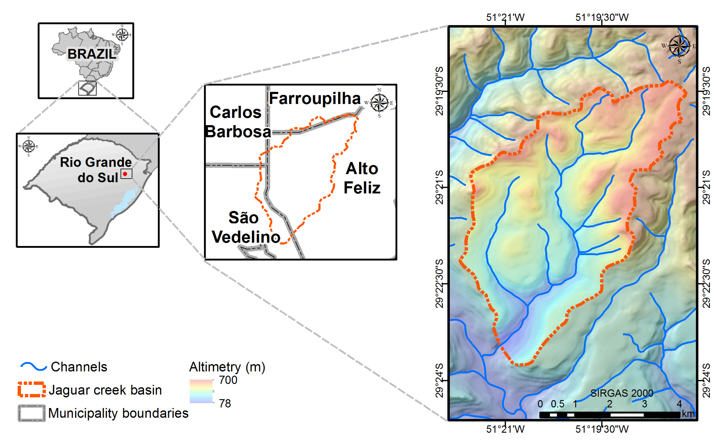
2.2. Study Area
2.3. Data
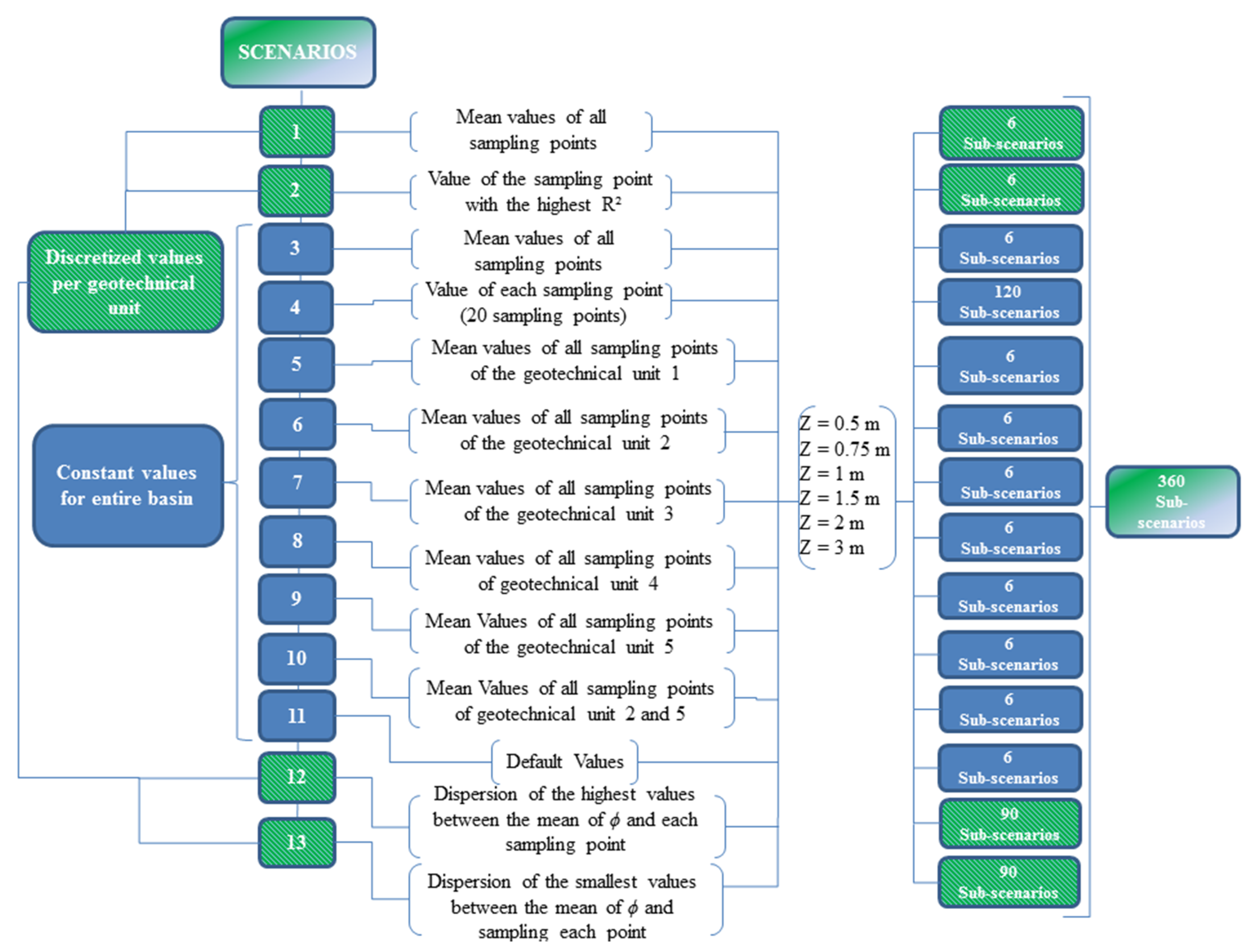
2.4. Application of the Modified SHALSTAB Model
2.5. Model Performance Assessment
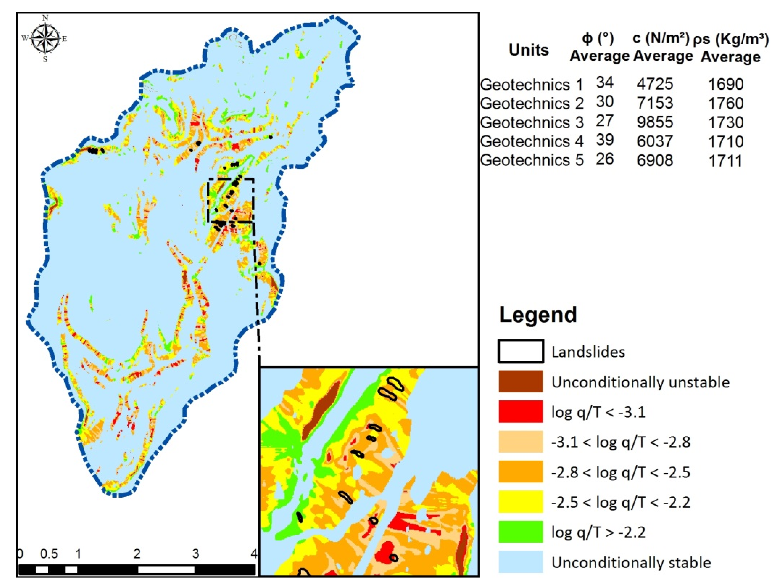
3. Results
4. Discussion
5. Conclusions
Author Contributions
Funding
Institutional Review Board Statement
Informed Consent Statement
Data Availability Statement
Conflicts of Interest
References
- Hamza, O.; De Vargas, T.; Boff, F.E.; Hussain, Y.; Sian Davies-Vollum, K. Geohazard Assessment of Landslides in South Brazil: Case Study. Geotech. Geol. Eng. 2019, 38, 971–984. [Google Scholar] [CrossRef]
- Luo, X.; Lin, F.; Chen, Y.; Zhu, S.; Xu, Z.; Huo, Z.; Yu, M.; Peng, J. Coupling logistic model tree and random subspace to predict the landslide susceptibility areas with considering the uncertainty of environmental features. Sci. Rep. 2019, 9, 1–13. [Google Scholar] [CrossRef] [Green Version]
- De Brito, M.M.; Weber, E.J.; Krigger, V.S.; Leitzke, F.P. Análise dos Fatores Condicionantes de Movimentos de Massa No Município de Porto Alegre a Partir de Registros Históricos. Rev. Bras. Cartogr. 2016, 68, 1853–1872. [Google Scholar]
- De Brito, M.M.; Weber, E.J.; Pinto da Silva Filho, L.C. Multi-Criteria Analysis Applied to Landslide Susceptibility Mapping. Rev. Bras. Geomorfol. 2017, 18, 919–935. [Google Scholar] [CrossRef] [Green Version]
- De Brito, M.M.; Weber, E.J.; Carlos, L.; Filho, S. Revista Brasileira de Geomorfologia Multi-Criteria Analysis Applied to Landslide Susceptibility Mapping Análise Multi-Critério Aplicada ao Mapeamento da. Rev. Bras. Geomorfol. 2017, 4, 719–735. [Google Scholar]
- Merghadi, A.; Yunus, A.P.; Dou, J.; Whiteley, J.; ThaiPham, B.; Bui, D.T.; Avtar, R.; Abderrahmane, B. Machine learning methods for landslide susceptibility studies: A comparative overview of algorithm performance. Earth-Sci. Rev. 2020, 207, 103225. [Google Scholar] [CrossRef]
- Montgomery, D.R.; Dietrich, W.E. A physically based model for the topographic control on shallow landsliding. Water Resour. Res. 1994, 30, 1153–1171. [Google Scholar] [CrossRef]
- Pack, R.; Tarboton, D.; Goodwin, C. SINMAP 2.0—A Stability Index Approach to Terrain Stability Hazard Mapping, User’s Manual; Utah State University: Logan, UT, USA, 1999. [Google Scholar]
- Iverson, R.M. Landslide triggering by rain infiltration. Water Resour. Res. 2000, 36, 1897–1910. [Google Scholar] [CrossRef] [Green Version]
- Baum, R.L.; Savage, W.Z.; Godt, J.W. TRIGRS—A Fortran program for transient rainfall infiltration and grid-based regional slope-stability analysis. Open-File Rep. 2002, 424, 38. [Google Scholar] [CrossRef] [Green Version]
- Corominas, J.; van Westen, C.; Frattini, P.; Cascini, L.; Malet, J.P.; Fotopoulou, S.; Catani, F.; Van Den Eeckhaut, M.; Mavrouli, O.; Agliardi, F.; et al. Recommendations for the quantitative analysis of landslide risk. Bull. Eng. Geol. Environ. 2014, 73, 209–263. [Google Scholar] [CrossRef]
- Zizioli, D.; Meisina, C.; Valentino, R.; Montrasio, L. Comparison between different approaches to modeling shallow landslide susceptibility: A case history in Oltrepo Pavese, Northern Italy. Nat. Hazards Earth Syst. Sci. 2013, 13, 559–573. [Google Scholar] [CrossRef] [Green Version]
- Vieira, B.C.; Fernandes, N.F.; Augusto Filho, O.; Martins, T.D.; Montgomery, D.R. Assessing shallow landslide hazards using the Trigrs and Shalstab models, Serra do Mar, Brazil. Environ. Earth Sci. 2018, 77, 1–15. [Google Scholar] [CrossRef]
- Michel, G.P.; Kobiyama, M.; Goerl, R.F. Comparative analysis of SHALSTAB and SINMAP for landslide susceptibility mapping in the Cunha River basin, southern Brazil. J. Soils Sediments 2014, 14, 1266–1277. [Google Scholar] [CrossRef]
- Rafaelli, S.G.; Montgomery, D.R.; Greenberg, H.M. A comparison of thematic mapping of erosional intensity to GIS-driven process models in an Andean drainage basin. J. Hydrol. 2001, 244, 33–42. [Google Scholar] [CrossRef]
- Goetz, J.N.; Guthrie, R.H.; Brenning, A. Integrating physical and empirical landslide susceptibility models using generalized additive models. Geomorphology 2011, 129, 376–386. [Google Scholar] [CrossRef]
- Teixeira, M.; Bateira, C.; Marques, F.; Vieira, B. Physically based shallow translational landslide susceptibility analysis in Tibo catchment, NW of Portugal. Landslides 2014, 12, 455–468. [Google Scholar] [CrossRef]
- Meisina, C.; Scarabelli, S. A comparative analysis of terrain stability models for predicting shallow landslides in colluvial soils. Geomorphology 2007, 87, 207–223. [Google Scholar] [CrossRef]
- Santini, M.; Grimaldi, S.; Nardi, F.; Petroselli, A.; Rulli, M.C. Pre-processing algorithms and landslide modelling on remotely sensed DEMs. Geomorphology 2009, 113, 110–125. [Google Scholar] [CrossRef]
- Sorbino, G.; Sica, C.; Cascini, L. Susceptibility analysis of shallow landslides source areas using physically based models. Nat. Hazards 2009, 53, 313–332. [Google Scholar] [CrossRef]
- Cando-Jácome, M.; Martínez-Graña, A. Determination of Primary and Secondary Lahar Flow Paths of the Fuego Volcano (Guatemala) Using Morphometric Parameters. Remote Sens. 2019, 11, 727. [Google Scholar] [CrossRef] [Green Version]
- Mazengarb, C. The Tasmanian Landslide Hazard Map Series: Methodology; Department of Infrastructure, Energy and Resources: Hobart, Australia, 2005. [Google Scholar]
- Guimaraes, R.F.; Montgomery, D.R.; Greenberg, H.M.; Fernandes, N.F.; Gomes, R.A.T.; de Carvalho Junior, O.A. Parameterization of soil properties for a model of topographic controls on shallow landsliding: Application to Rio de Janeiro. Eng. Geol. 2003, 69, 99–108. [Google Scholar] [CrossRef]
- Gomes, R.A.T.; Guimarães, R.F.; Osmar Abílio De Carvalho, J.; Fernandes, N.F.; Júnior, E.V.D.A. Combining Spatial Models for Shallow Landslides and Debris-Flows Prediction. Remote Sens. 2013, 5, 2219–2237. [Google Scholar] [CrossRef] [Green Version]
- Paulo Michel, G.; Kobiyama, M.; Fabris Goerl, R. Formulação do fator de segurança considerando a presença de vegetação. In Proceedings of the XX Brazilian Symposium on Water Resources, Bento Gonçalves, Brazil, 17–22 November 2013; Volume 8. (In Portuguese). [Google Scholar]
- Michel, G.P.; Kobiyama, M.; Goerl, R.F.; Zanandrea, F.; Paul, L.R.; Schwarz, H.; Cardozo, G.L. Efeitos da vegetação na modelagem de estabilidade de encostas na bacia hidrográfica do rio Cunha, Santa Catarina. Rev. Bras. Geomorfol. 2021, 22, 824–846. [Google Scholar] [CrossRef]
- Martins, T.D.; Vieira, B.C.; Fernandes, N.F.; Okafiori, C.; Montgomery, D.R. Application of the Shalstab model for the identification of areas susceptible to landslides: Brazilian case studies. Rev. Geomorfol. 2017, 19, 136–144. [Google Scholar] [CrossRef]
- Sbroglia, R.M.; Reginatto, G.M.P.; Higashi, R.A.R.; Guimarães, R.F. Mapping susceptible landslide areas using geotechnical homogeneous zones with different DEM resolutions in Ribeirão Baú basin, Ilhota/SC/Brazil. Landslides 2018, 15, 2093–2106. [Google Scholar] [CrossRef]
- Dos Santos, E.M.; Listo, F.D.L.R. Escorregamentos translacionais rasos no município de Camaragibe, região metropolitana do Recife: Uma análise preliminar a partir do modelo SHALSTAB. Rev. Geociências Nord. 2019, 5, 131–145. [Google Scholar] [CrossRef]
- Pacheco, T.C.K.F.; Kux, H.J.H.; Mendes, R.M. Identificação de Áreas de Suscetibilidade a Escorregamentos de Encosta Utilizando o Modelo Matemático Shalstab. Bol. Geogr. 2020, 37, 228–243. [Google Scholar] [CrossRef]
- Guimarães, R.F.; Machado, W.P.; De Carvalho, O.A.; Montgomery, D.R.; Gomes, R.A.T.; Greenberg, H.M.; Cataldi, M.; Mendonça, P.C. Determination of Areas Susceptible to Landsliding Using Spatial Patterns of Rainfall from Tropical Rainfall Measuring Mission Data, Rio de Janeiro, Brazil. ISPRS Int. J. Geo-Inf. 2017, 6, 289. [Google Scholar] [CrossRef] [Green Version]
- Melo, C.M.; Kobiyama, M. Aplicação do Modelo Shalstab No Estudo de Escorregamentos No Brasil: Revisão. Rev. Bras. Geomorfol. 2018, 19, 4. [Google Scholar] [CrossRef]
- Tarolli, P.; Borga, M.; Chang, K.T.; Chiang, S.H. Modeling shallow landsliding susceptibility by incorporating heavy rainfall statistical properties. Geomorphology 2011, 133, 199–211. [Google Scholar] [CrossRef]
- König, T.; Kux, H.J.H.; Mendes, R.M. Shalstab mathematical model and WorldView-2 satellite images to identification of landslide-susceptible areas. Nat. Hazards 2019, 97, 1127–1149. [Google Scholar] [CrossRef]
- Kim, M.S.; Onda, Y.; Uchida, T.; Kim, J.K. Effects of soil depth and subsurface flow along the subsurface topography on shallow landslide predictions at the site of a small granitic hillslope. Geomorphology 2016, 271, 40–54. [Google Scholar] [CrossRef]
- Dias, R.D. Proposta de metodologia de definição de carta geotécnica básica em regiões tropicais e subtropicais. Rev. Inst. Geológico 1995, 16, 51–55. [Google Scholar] [CrossRef] [Green Version]
- Zhang, W.; Montgomery, D.R. Digital elevation model grid size, landscape representation, and hydrologic simulations. Water Resour. Res. 1994, 30, 1019–1028. [Google Scholar] [CrossRef]
- Borga, M.; Fontana, G.D.; Gregoretti, C.; Marchi, L. Assessment of shallow landsliding by using a physically based model of hillslope stability. Hydrol. Process. 2002, 16, 2833–2851. [Google Scholar] [CrossRef]
- Zweig, M.H.; Campbell, G. Receiver-operating characteristic (ROC) plots: A fundamental evaluation tool in clinical medicine. Clin. Chem. 1993, 39, 561–577. [Google Scholar] [CrossRef] [PubMed]
- Giri, S.; Qiu, Z.; Prato, T.; Luo, B. An Integrated Approach for Targeting Critical Source Areas to Control Nonpoint Source Pollution in Watersheds. Water Resour. Manag. 2016, 30, 5087–5100. [Google Scholar] [CrossRef]
- Sarkar, S.; Roy, A.K.; Raha, P. Deterministic approach for susceptibility assessment of shallow debris slide in the Darjeeling Himalayas, India. CATENA 2016, 142, 36–46. [Google Scholar] [CrossRef]
- Coelho, F.F.; Giasson, E.; Campos, A.R.; de Oliveira e Silva, R.G.P.; Costa, J.J.F. Geographic object-based image analysis and artificial neural networks for digital soil mapping. CATENA 2021, 206, 105568. [Google Scholar] [CrossRef]
- Michel, G.P. Estimativa da Profundidade do Solo e Seu Efeito na Modelagem de Escorregamentos; Universidade Federal do Rio Grande do Sul: Porto Alegre, Brazil, 2015. [Google Scholar]
- Kobiyama, M.; Michel, R.D.L.; Paixão, M.A.; Michel, G.P. Small Fish-pond Design for Debris Flow Disaster Measure with Kanako-2D. In Proceedings of the Symposium Proceedings of the INTERPRAENENT 2018 in the Pacific Rim, Toyama, Japan, 1–4 October 2018; pp. 264–269. [Google Scholar]
- Vanacôr, R.N.; Rolim, S.B.A. Mapeamento da Suscetibilidade a Deslizamentos Usando Técnicas de Estatística Bivariada e Sistema de Informações Geográficas na Região Nordeste do Rio Grande do Sul. Rev. Bras. Geomorfol. 2012, 13, 1. [Google Scholar] [CrossRef] [Green Version]
- Van Den Eeckhaut, M.; Vanwalleghem, T.; Poesen, J.; Govers, G.; Verstraeten, G.; Vandekerckhove, L. Prediction of landslide susceptibility using rare events logistic regression: A case-study in the Flemish Ardennes (Belgium). Geomorphology 2006, 76, 392–410. [Google Scholar] [CrossRef]
- Beguería, S. Validation and Evaluation of Predictive Models in Hazard Assessment and Risk Management. Nat. Hazards 2006, 37, 315–329. [Google Scholar] [CrossRef] [Green Version]
- Dietrich, W.E.; Bellugi, D.; Real de Asua, R. Validation of the Shallow Landslide Model, SHALSTAB, for forest management. Water Sci. Appl. 2001, 2, 195–227. [Google Scholar] [CrossRef]


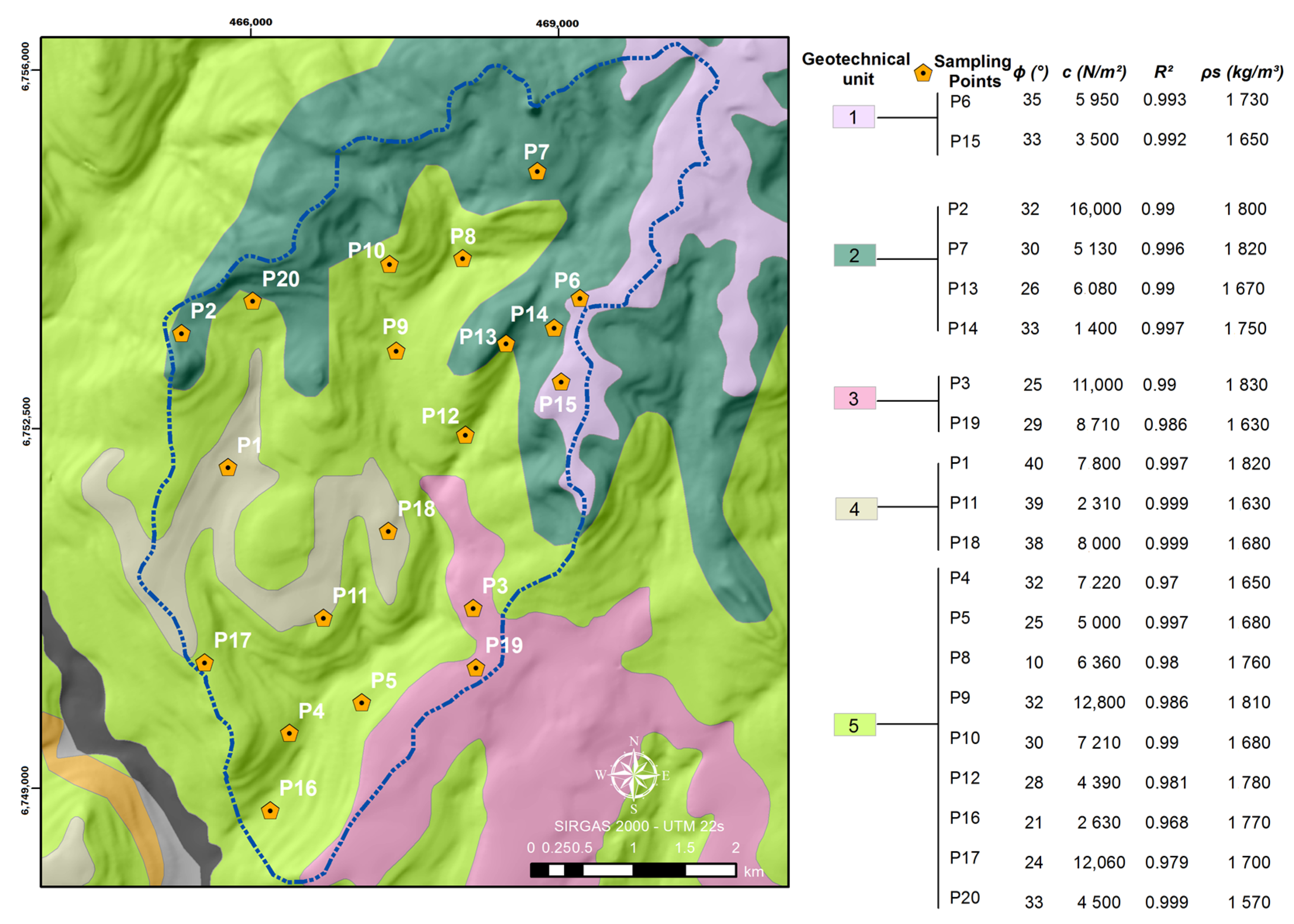
| Geotechnical Unit | Lithology | Soil Type |
|---|---|---|
| 1 | Facies Caxias | Cambisol |
| 2 | Facies Caxias | Neosoil |
| 3 | Facies Gramado | Chernozem |
| 4 | Facies Gramado | Nitosol |
| 5 | Facies Gramado | Neosoil |
| Geotechnical Unit | ||||||
|---|---|---|---|---|---|---|
| 1 | 2 | 3 | 4 | 5 | ||
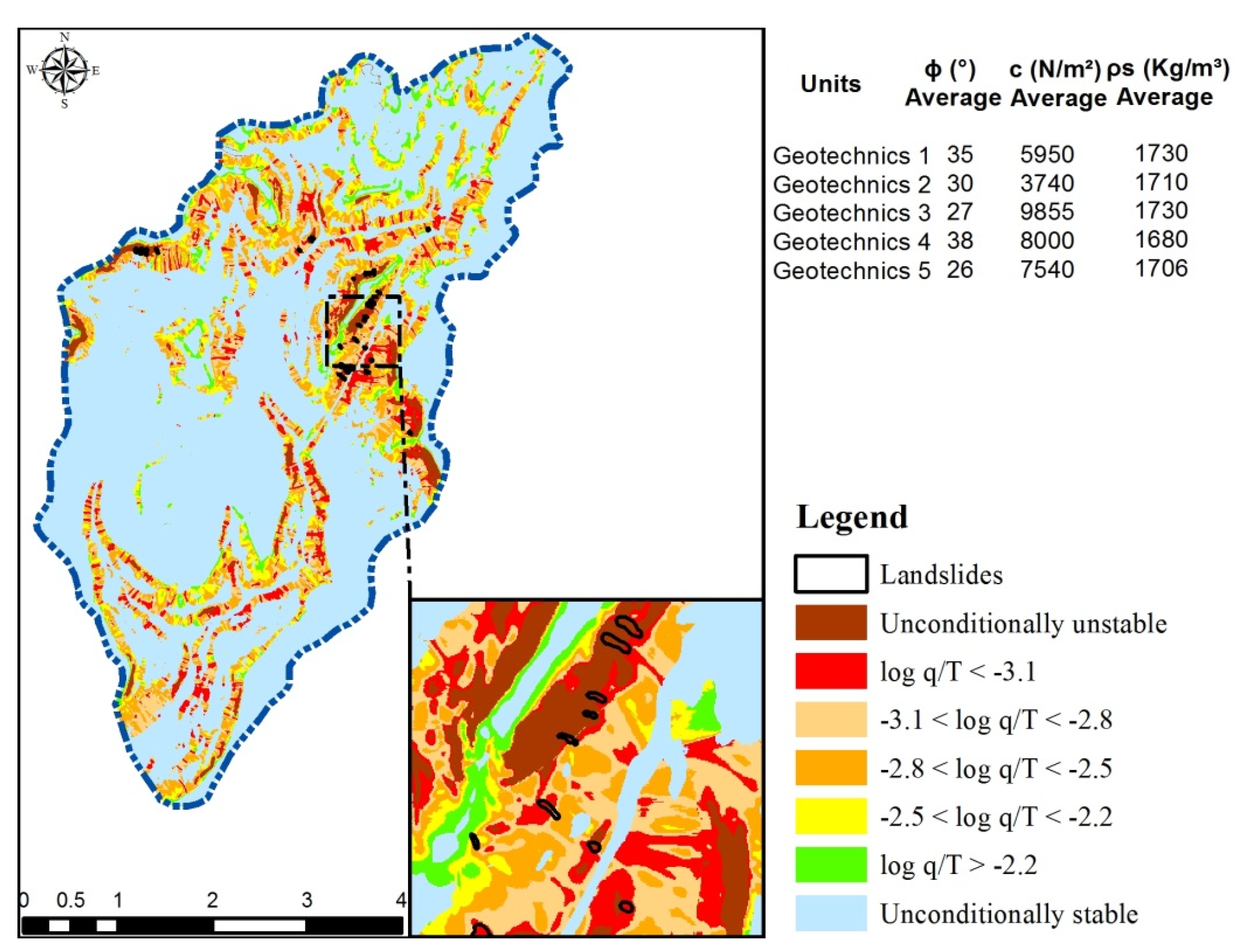
| Scenario 1 | Average ϕ (°) | 34 | 30 | 27 | 39 | 26 |
| Average c (N/m2) | 4725 | 7153 | 9855 | 6037 | 6908 | |
| Average ρs (kg/m3) | 1690 | 1760 | 1730 | 1710 | 1711 | |
| Average Ks (m/s) | 2.05 × 10⁻⁴ | 1.85 × 10⁻⁴ | 2.14 × 10⁻⁴ | 2.56 × 10⁻⁴ | 2.68 × 10⁻⁴ | |
| Scenario 2 | Sampling point | P6 | P14 | P3 | P18 | P20 |
| R2 | 0.993 | 0.997 | 0.99 | 0.999 | 0.999 | |
| ϕ (°) | 35 | 33 | 25 | 38 | 33 | |
| c (N/m2) | 5950 | 1400 | 11,000 | 8000 | 4500 | |
| Ks (m/s) | 1.9 × 10⁻⁴ | 2.0 × 10⁻⁴ | 7.7 × 10⁻⁵ | 2.8 × 10⁻⁴ | 6.3 × 10⁻⁴ | |
| Scenario 3 | Average ϕ (°) | 30 | 30 | 30 | 30 | 30 |
| Average c (N/m2) | 6903 | 6903 | 6903 | 6903 | 6903 | |
| Average ρs (kg/m3) | 1721 | 1721 | 1721 | 1721 | 1721 | |
| Average Ks (m/s) | 2.38 × 10⁻⁴ | 2.38 × 10⁻⁴ | 2.38 × 10⁻⁴ | 2.38 × 10⁻⁴ | 2.38 × 10⁻⁴ | |
| Scenario 11 | Average ϕ (°) | 45 | 45 | 45 | 45 | 45 |
| Average c (N/m2) | 2000 | 2000 | 2000 | 2000 | 2000 | |
| Average ρs (kg/m3) | 1600 | 1600 | 1600 | 1600 | 1600 | |
| Sampling Point | Φ (°) | c (N/m2) | ρs (kg/m3) | Ks (m/s) |
|---|---|---|---|---|
| P1 | 40 | 7800 | 1820 | 8.9 × 10⁻⁵ |
| P2 | 32 | 16,000 | 1800 | 1.2 × 10⁻⁴ |
| P3 | 25 | 11,000 | 1830 | 7.7 × 10⁻⁵ |
| P4 | 32 | 7220 | 1650 | 3.9 × 10⁻⁴ |
| P5 | 25 | 5000 | 1680 | 2.6 × 10⁻⁴ |
| P6 | 35 | 5950 | 1730 | 1.9 × 10⁻⁴ |
| P7 | 30 | 5130 | 1820 | 1.1 × 10⁻⁴ |
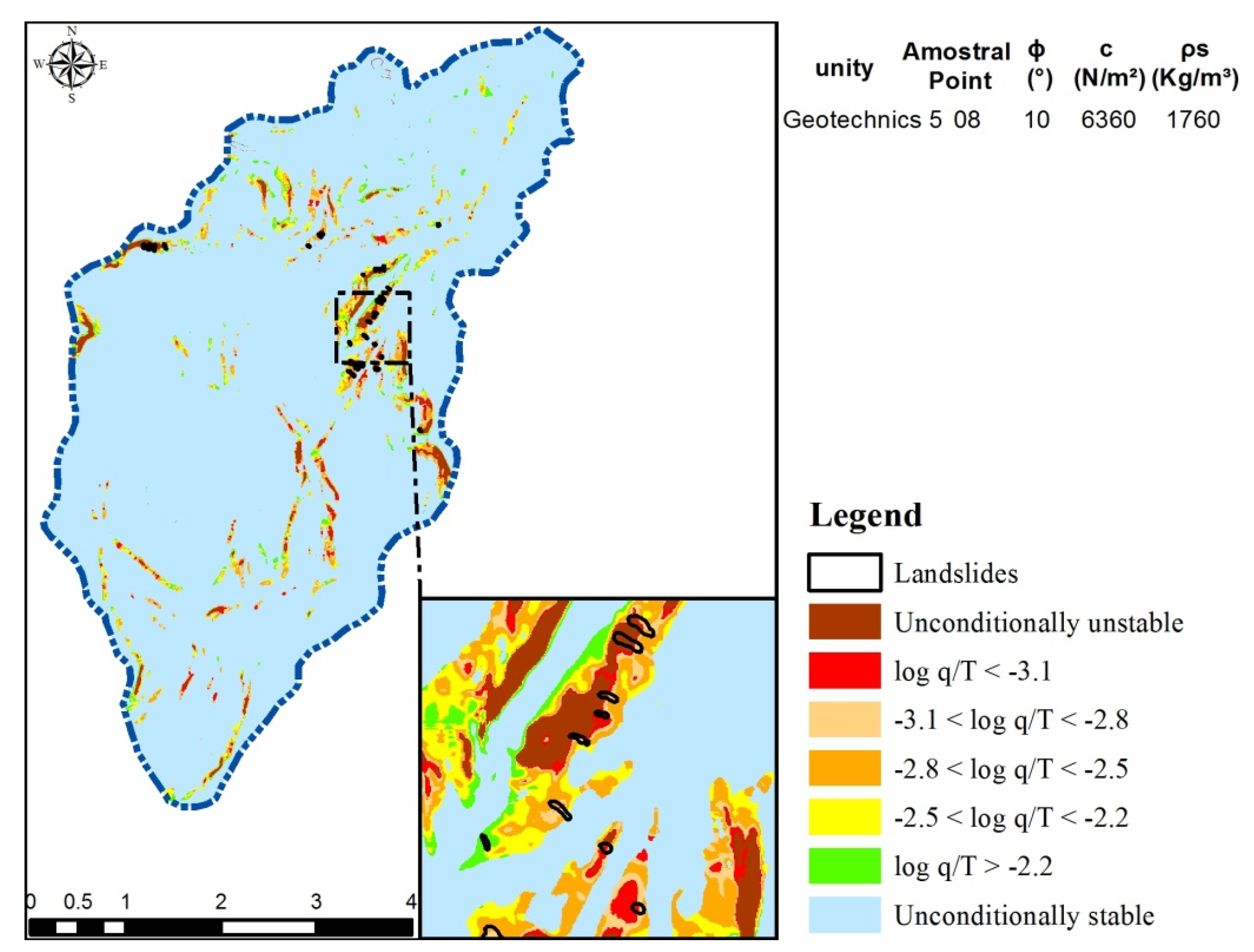
| P8 | 10 | 6360 | 1760 | 1.7 × 10⁻⁴ |
| P9 | 32 | 12,800 | 1810 | 8.1 × 10⁻⁵ |
| P10 | 30 | 7210 | 1680 | 2.5 × 10⁻⁴ |
| P11 | 39 | 2310 | 1630 | 4.0 × 10⁻⁴ |
| P12 | 28 | 4390 | 1780 | 1.8 × 10⁻⁴ |
| P13 | 26 | 6080 | 1670 | 3.1 × 10⁻⁴ |
| P14 | 33 | 1400 | 1750 | 2.0 × 10⁻⁴ |
| P15 | 33 | 3500 | 1650 | 3.2 × 10⁻⁴ |
| P16 | 21 | 2630 | 1770 | 1.2 × 10⁻⁴ |
| P17 | 24 | 12,060 | 1700 | 3.3 × 10⁻⁴ |
| P18 | 38 | 8000 | 1680 | 2.8 × 10⁻⁴ |
| P19 | 29 | 8710 | 1630 | 3.5 × 10⁻⁴ |
| P20 | 33 | 4500 | 1570 | 6.3 × 10⁻⁴ |
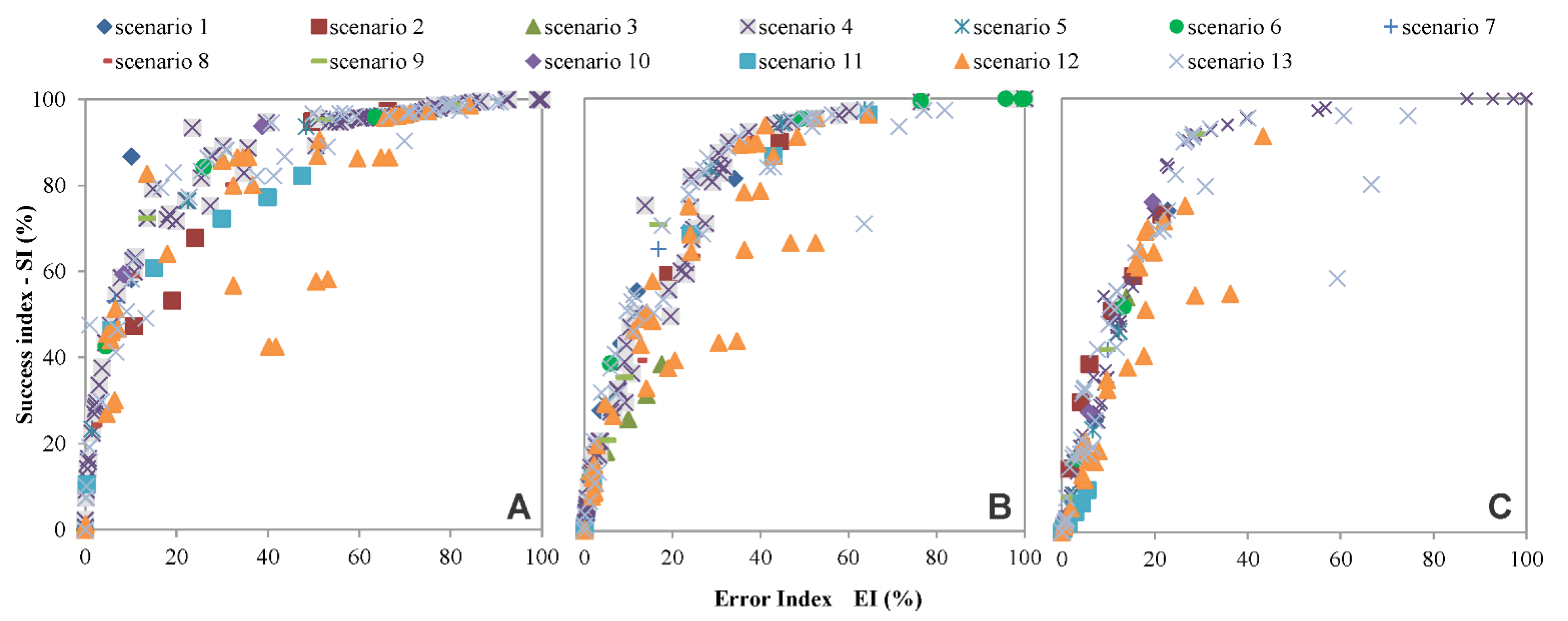
| Scenario | 5 | 6 | 7 | 8 | 9 | 10 |
| Geotechnical Unit | 1 | 2 | 3 | 4 | 5 | 2 and 5 |
| No. of Sample Points | 2 | 4 | 2 | 3 | 9 | 13 |
| Φ (°) | 34 | 30 | 27 | 39 | 26 | 28 |
| c (N/m2) | 4725 | 7153 | 9855 | 6037 | 6908 | 6983 |
| ρs (kg/m3) | 1690 | 1760 | 1730 | 1710 | 1711 | 1726 |
| Geotechnical Unit | Point | ϕ (°) | Dispersal | Withdrawal Order Scenario 12 | Withdrawal Order Scenario 13 | |
|---|---|---|---|---|---|---|
| 1 | P6 | 35 | 34 | 1.1 | 15° | |
| P15 | 33 | 3° | ||||
| 2 | P2 | 32 | 30 | 1.5 | 12° | 6° |
| P7 | 30 | 0.37 | 2° | |||
| P13 | 26 | 4 | 6° | |||
| P14 | 33 | 3 | 8° | 10° | ||
| 3 | P3 | 25 | 27 | 2.34 | 10° | |
| P19 | 29 | 8° | ||||
| 4 | P1 | 40 | 39 | 1.14 | 14° | 4° |
| P11 | 39 | 0.16 | 1° | |||
| P18 | 38 | 1 | 13° | |||
| 5 | P4 | 32 | 26 | 6 | 3° | 14° |
| P5 | 25 | 1.14 | 5° | |||
| P8 | 10 | 16 | 1° | |||
| P9 | 32 | 5 | 4° | 13° | ||
| P10 | 30 | 4 | 7° | 11° | ||
| P12 | 28 | 2 | 11° | 7° | ||
| P16 | 21 | 5 | 5° | 12° | ||
| P17 | 24 | 2 | 9° | 9° | ||
| P20 | 33 | 7 | 2° | 15° |
| ID | Classes |
|---|---|
| 1 | Unconditionally instable |
| 2 | log q/T < −3.1 |
| 3 | −3.1 < log q/T < −2.8 |
| 4 | −2.8 < log q/T < −2.5 |
| 5 | −2.5 < log q/T < −2.2 |
| 6 | −2.2 < log q/T |
| 7 | Unconditionally stable |
Publisher’s Note: MDPI stays neutral with regard to jurisdictional claims in published maps and institutional affiliations. |
© 2021 by the authors. Licensee MDPI, Basel, Switzerland. This article is an open access article distributed under the terms and conditions of the Creative Commons Attribution (CC BY) license (https://creativecommons.org/licenses/by/4.0/).
Share and Cite
Melo, C.M.; Kobiyama, M.; Michel, G.P.; de Brito, M.M. The Relevance of Geotechnical-Unit Characterization for Landslide-Susceptibility Mapping with SHALSTAB. GeoHazards 2021, 2, 383-397. https://doi.org/10.3390/geohazards2040021
Melo CM, Kobiyama M, Michel GP, de Brito MM. The Relevance of Geotechnical-Unit Characterization for Landslide-Susceptibility Mapping with SHALSTAB. GeoHazards. 2021; 2(4):383-397. https://doi.org/10.3390/geohazards2040021
Chicago/Turabian StyleMelo, Carla Moreira, Masato Kobiyama, Gean Paulo Michel, and Mariana Madruga de Brito. 2021. "The Relevance of Geotechnical-Unit Characterization for Landslide-Susceptibility Mapping with SHALSTAB" GeoHazards 2, no. 4: 383-397. https://doi.org/10.3390/geohazards2040021
APA StyleMelo, C. M., Kobiyama, M., Michel, G. P., & de Brito, M. M. (2021). The Relevance of Geotechnical-Unit Characterization for Landslide-Susceptibility Mapping with SHALSTAB. GeoHazards, 2(4), 383-397. https://doi.org/10.3390/geohazards2040021