Research on the Prediction of Greenhouse Temperature and Humidity Using an IPSO-LSTM Model

Abstract

This paper presents a study on the prediction of greenhouse temperature and humidity using an improved particle swarm optimization (IPSO) algorithm combined with a long short-term memory (LSTM) neural network, namely IPSO-LSTM. Accurate environmental prediction is crucial for modern protected agriculture, but traditional LSTM models often suffer from suboptimal hyperparameter tuning. To address this, we propose an IPSO-LSTM model where an improved PSO with a linearly decreasing inertia weight is employed to automatically search for the optimal hyperparameters of the LSTM. Experimental results based on hourly data collected from a Venlo-type glass greenhouse over a 90-day period demonstrate the superiority of the proposed model. Specifically, in the tomato scenario, the IPSO-LSTM achieved an R² of 0.9969 for temperature and 0.9967 for humidity, with MAPE values as low as 0.0118 and 0.0127, respectively. These results indicate that the IPSO-LSTM model significantly outperforms conventional LSTM and standard PSO-LSTM models, providing a reliable tool for intelligent greenhouse climate control.

1. Introduction

Greenhouses play an essential role in contemporary agriculture, offering a dependable means for crop cultivation [1]. The development of modern agriculture benefits from the progress of science and technology. The focus of modern agriculture is on maximizing yields and efficiency, and leveraging technology. The greenhouse is a prime illustration of this modern approach to agriculture [2]. However, the precise regulation of the greenhouse environment is complicated by the non-linearity, large inertia, strong coupling, and large time delay of the greenhouse environment factors [3]. To address the greenhouse’s time lag issue, more precise control of the crop growth environment must be anticipated in advance based on the changing state of the greenhouse environment [4]. Temperature and humidity are significant factors in crop growth because they are the primary influencing factors in greenhouses [5]. It is possible to produce greenhouse crops with a high yield, high efficiency, and high quality by optimizing the control mode of greenhouse temperature and humidity [6].

The neural network methods commonly used for time-series forecasting include the perceptron model, backpropagation algorithm (BP), Recurrent Neural Network (RNN), and long short-term memory (LSTM). In current times, artificial neural network prediction models find primary applications in sectors such as architecture, electricity, energy, and water resources. Arsenault et al. [7] employed an LSTM predictive model to forecast watershed flow rates, comparing its performance against traditional hydrological models. Their findings demonstrate that the LSTM predictive model significantly enhances the precision of water flow rate predictions in the studied water bodies. Chen et al. [8] addressed the challenge of obtaining the magnitude and variation trends of insertion resistance during loader pile insertion. They proposed a combined model based on the particle swarm optimization (PSO) algorithm and LSTM network to tackle this issue. Comparing it with the LSTM prediction model, the PSO-LSTM model demonstrated superior predictive accuracy. During the laser solid forming process, the temperature of the molten pool significantly impacts the precision and performance of parts. Wang et al. [9] developed a molten pool temperature prediction model based on PSO-LSTM, enabling accurate forecasting of the molten pool temperature. Jiao et al. [10] utilized a PSO-LSTM combined predictive model to forecast the volatility in the crude oil market, demonstrating notable predictive accuracy. Mu et al. [11] constructed an IPSO-LSTM hybrid forecasting model to predict sudden network public opinion events. Huang et al. [12] introduced a wind power prediction model based on IPSO-LSTM. Through case studies, this model demonstrates proficient forecasting of wind power output. PSO-enhanced models are important for hybrid prediction methods. Khatir et al. [13] proposed a new hybrid algorithm combining particle swarm optimization and YUKI (PSO-YUKI). The model has high computational performance for damage identification. PSO-YUKI is robust to double crack depth recognition compared to PSO. Khatir et al. [14] proposed a hybrid ANN-RSA model to improve the accuracy of damage location prediction. The results show that the RSA method effectively optimizes the ANN parameters and improves the reliability and accuracy of damage localization. Khatir et al. [15] improved ANN training using the Finite Element Method (FEM) and an artificial neural network (ANN) combined with the Butterfly Optimization Algorithm (BOA). The results show that the proposed method can predict the crack depth more accurately.

With the development of artificial neural network technology, artificial neural network models have been increasingly used to address agricultural issues [16]. Liu et al. [17] proposed the GCP_LSTM model for greenhouse climate prediction, accurately forecasting six climate factors affecting crop growth, such as temperature, humidity, light intensity, carbon dioxide concentration, and soil temperature and humidity. Because a single artificial intelligence algorithm cannot adapt to dynamic changes, Ullah et al. [18] proposed a learning module based on an artificial neural network to support autonomous environmental monitoring and control, resulting in an energy-saving improvement of 11.73% according to experimental comparisons. Gao et al. [19] proposed a time-series-based model for predicting daylight greenhouse temperature using the non-linear autoregressive exogenous (NARX) method; the results show that the maximum absolute error of the model is 0.67 °C, which can accurately predict the temperature trend inside the daylight greenhouse. Mohammadi et al. [20] developed hybrid models, namely multi-layer perceptron (MLP)-linear autoregressive (AR), AR-autoregressive conditional heteroscedasticity (ARCH), and MLP-AR-ARCH, by coupling AR, ARCH, and MLP models. These combined models were compared with single AR and MLP predictive models. Findings revealed that the MLP-AR temperature prediction model exhibited the highest level of accuracy among the studied models. Mohammadi et al. [21] proposed a hybrid model combining artificial neural networks with a state-of-the-art firefly algorithm for predicting the Standardized Precipitation Index at different time scales. The results demonstrate that this hybrid model is an effective and promising method for drought prediction. A comparative summary between existing studies and the proposed model is listed in

Table 1. Comparative analysis between this study and existing research.

Model	${\mathit{R}}^2$ (Temperature)	${\mathit{R}}^2$ (Humidity)	Advantages	Disadvantages
Standard LSTM	~0.95	~0.89	Strong long-term dependency capture	Manual tuning prone to local optima
PSO-LSTM	~0.97	~0.93	Automated tuning, better accuracy	Premature convergence, weak global search
SSA-LSTM	~0.98	~0.95	Fast convergence, high efficiency	High computational cost, poor noise robustness
IPSO-LSTM (Proposed)	0.9969	0.9967	Highest accuracy, balanced search	Relatively high computational demand

.

Compared to traditional neural networks, LSTM models possess gated mechanisms that enable them to learn and retain long-term dependencies, addressing the issue of long-range dependencies present in RNNs. However, the establishment of an LSTM model requires many experiments, and the effective parameters are selected for prediction through experience. This method requires a large number of experiments and has poor reliability in parameter acquisition, so it is difficult to quickly obtain the best parameters. The IPSO algorithm [22] provides a solution for finding optimal parameters, can effectively take into account the global exploration and local mining capabilities, and has the advantages of fast convergence, high accuracy, and avoiding the local optimal solution. Therefore, this paper introduces the IPSO algorithm to optimize LSTM model parameters to predict the greenhouse temperature and humidity. The main work is summarized as follows:

(1) Comparison of different prediction models: The study compared the prediction performance of three different prediction models, IPSO-LSTM, PSO-LSTM, and LSTM, on the environmental temperature and humidity of tomato and cucumber crops, and put forward the optimal model.

(2) Detailed investigation of the optimal model: The selected optimal model is thoroughly investigated by varying the volume of the training sample; the study verifies the influence of different training sample volumes on the accuracy of greenhouse environment predictions.

2. Mathematical Model and Evaluation Method

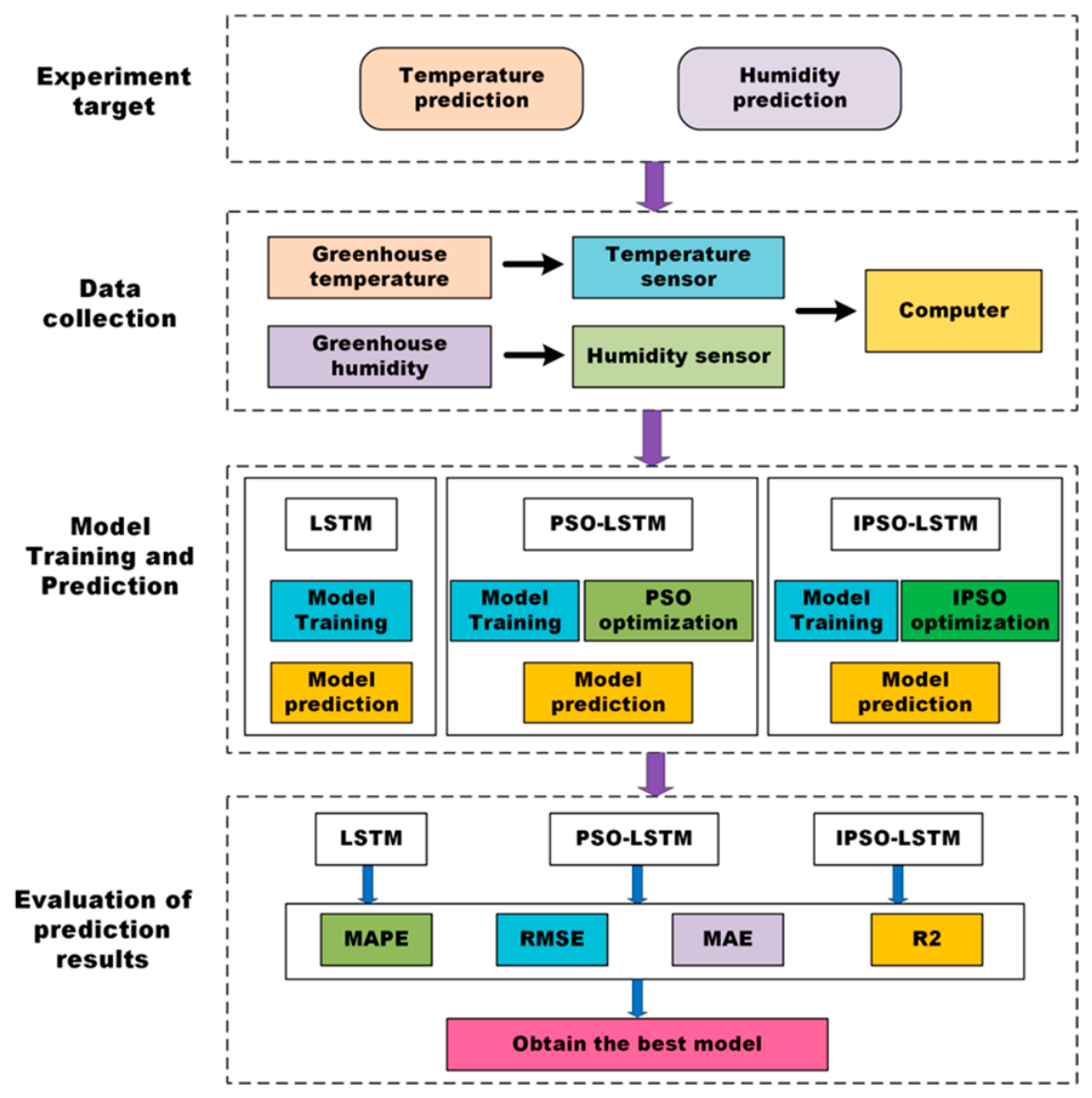
This section primarily introduces the LSTM prediction model, PSO and IPSO optimization algorithms, and model evaluation parameters. It also proposes the IPSO-LSTM combined prediction model. Figure 1 outlines the entire research workflow.

2.1. Particle Swarm Optimization (PSO)

PSO is a population-based stochastic optimization algorithm proposed by Kennedy and Eberhart in 1995, inspired by observations of animal social behavior. This algorithm achieves the global optimal solution by sharing the position and velocity of each particle within the population. The following outlines the fundamental principles of this algorithm.

(1) Assuming a population size of N, each particle exists in a D-dimensional space. The position of the $i$ particle is denoted as $x_i=[x_{i1}, x_{i2},\cdots , x_{iD}], i=1,2,\cdots ,N$, where $x_{iD}(t)$ represents the position of the $i$ particle in a D-dimensional space at time $t$. Assuming the velocity of the $i$ particle is $v_i=[v_{i1}, v_{i2},\cdots , v_{iD}], i=1,2,\cdots ,N$, $p_{best}=[p_{i1}, p_{i2},\cdots , p_{iD}], i=1,2,\cdots ,N$ represents the best individual position found by the $i$ particle in the solution space, and $g_{best}=[p_{g1}, p_{g2},\cdots , p_{gD}], i=1,2,\cdots ,N$ denotes the best position discovered by the entire population.

(2) Particle and population best values are utilized to update particle velocity and position, as expressed in Equations (1) and (2):

$$v_{ij}\left(t+1\right)=v_{ij}\left(t\right)+c_1{r}_1\left[p_{ij}\left(t\right)-x_{ij}\left(t\right)\right]+c_2{r}_2(t)[p_{gj}(t)-x_{ij}(t)]$$

(1)

$$x_{ij}(t+1)=x_{ij}(t)+v_{ij}(t+1)$$

(2)

Here, where $j=1,2,\cdots ,D$, $i=1,2,\cdots ,N$, $t$ represents the iteration count; $v_{ij}$ stands for the velocity of the $i$ particle in the $j$ dimension; $x_{ij}$ denotes the position of the $i$ particle in the $j$ dimension; the learning factors $c_1$ and $c_2$ are non-negative constants; the random numbers $r_1$ and $r_2$ range between 0 and 1.

2.2. Improved Particle Swarm Optimization (IPSO)

The IPSO is a population-based stochastic search algorithm [23] that optimizes the PSO [24] by modifying the inertia weight coefficient $w$. The inertia weight coefficient $w$ reflects the particles’ ability to inherit their previous velocities, where a higher inertia weight value favors global exploration, and a smaller value favors local exploitation. By employing a linearly decreasing inertia weight, IPSO achieved a better balance between global and local search capabilities and avoided the issue of being trapped in local optima. Through continuous iterations, IPSO updated its velocity and position to search for the optimal parameters of the prediction model and ultimately found the best-fit parameters.

The velocity and position updates are given by the following Equations (3) and (4):

$$v_{ij}\left(t+1\right)=w{v}_{ij}\left(t\right)+c_1{r}_1\left[p_{ij}\left(t\right)-x_{ij}\left(t\right)\right]+c_2{r}_2(t)[p_{gj}(t)-x_{ij}(t)]$$

(3)

$$x_{ij}(t+1)=x_{ij}(t)+v_{ij}(t+1)$$

(4)

The inertia weight coefficient $w$ is updated according to Equation (3):

$$w=w_{\max }-{\displaystyle \frac{\left(w_{\max }-w_{\min }\right)\ast T}{T_{\max }}}$$

(5)

where $T_{\max }$ is the maximum number of iterations; $w_{\max }$ is the maximum inertia weight; $w_{\min }$ is the minimum inertia weight; $T$ is the current iteration number.

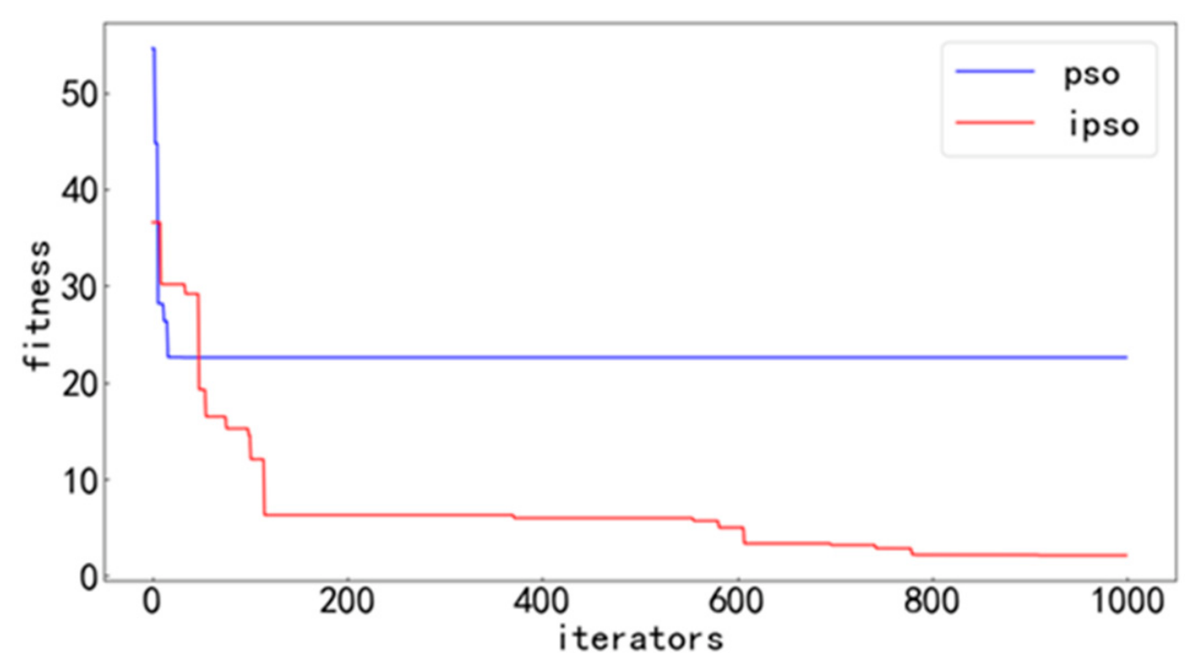
To verify the optimization performance of IPSO, the fitness function is introduced to test and compare the performance of PSO and IPSO algorithms. The fitness function is shown in Equation (6), and the IPSO and PSO algorithms are optimized. The number of iterations is 1000. The parameter settings are shown in

Table 2. Comparison of IPSO and PSO parameter settings.

Parameter	IPSO	PSO
dimensional	3	3
learning rate	0.001~0.01	0.001~0.01
learning factor C1 and C2	1.5, 1.5	1.5, 1.5
weight coefficient	0.2~0.8	0.8
random number r1 and r2	0.8, 0.3	0.8, 0.3
population size	50	50
Hidden layer neuron range	10~200	10~200

:

$$f={\displaystyle \sum _{i=1}^n[{x_i}^2-10\cos (2\pi x_i)+10],x_i\in [-5.12,5.12]}$$

(6)

The comparison of fitness curves between PSO and IPSO is shown in Figure 2. It can be seen that the ability of the IPSO algorithm to find the individual optimal fitness is obviously better than that of the PSO algorithm, and the accuracy of the individual optimal fitness obtained by convergence of the IPSO algorithm is obviously lower than that of the PSO algorithm under a certain number of iterations. PSO algorithm falls into local convergence at the beginning of the iterations, while the IPSO algorithm can jump out of local convergence and, finally, reach optimal convergence with the increase in iteration times. This shows that the IPSO algorithm has stronger search ability.

While optimizing LSTM with swarm intelligence is an established approach, the specific scientific innovation here lies in addressing the unique large inertia and high-frequency fluctuations of greenhouse microclimates. Conventional PSO often converges prematurely into local optima when confronted with the dynamic non-linearity of greenhouse data. The IPSO algorithm specifically overcomes this by utilizing a linearly decreasing inertia weight, which perfectly matches the required shifting balance: prioritizing global exploration to capture sudden weather-induced temperature spikes, and transitioning to fine-grained local exploitation to track subtle humidity variations caused by crop transpiration. This targeted adaptability makes IPSO significantly more robust for this specific agricultural application than conventional PSO.

2.3. Long Short-Term Memory Model

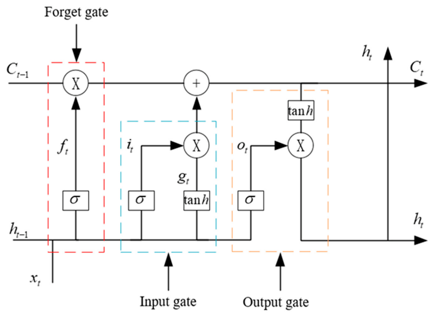
The LSTM model consists of three gates: the forget gate, the input gate, and the output gate. Firstly, the forget gate determines how much of the previous time step’s cell state should be retained at the current time step. The input gate determines how much of the current time step’s input should be stored in the cell state. Lastly, the output gate regulates how much of the controlled cell state should be output to the current output value of the LSTM. $C_{t-1}$ represents the cell state from the previous time step; $C_t$ represents the information from the output gate at the previous time step; $h_t$ represents the information from the current output gate; $x_t$ represents the external stimulus information from $x$ at time step $t$; after passing through the sigmoid function, both $h_{t-1}$ and $x_t$ generate the value $f_t$, the information flow acting on the forget gate. $i_t$ is the information flow generated when $x_t$ is activated by the sigmoid function; $\tanh$ represents the activation function; $g_t$ represents the information flow obtained after merging $h_{t-1}$ and $x_t$ through the $\tanh$-layer. The combined effect of $C_{t-1}$, $f_t$, $i_t$ and $g_t$ generates a new information flow; $o_t$ represents the information flow obtained when $h_{t-1}$ and $x_t$ are activated by the sigmoid function and act on the output gate [25]. The process is shown in Figure 3.

The calculation process of the forget gate is as follows: The forget gate determines whether to discard or retain information. The output value from the previous unit is denoted as $h_{t-1}$. The current unit’s input values $x_t$ and $\sigma$ jointly produce a value in the range of [0, 1]. This value is used to determine the importance of information, where 0 indicates that the information is not important, and 1 indicates that the information is important. The output value $h_{t-1}$ from the previous unit and the input value $x_t$ of the current unit are both involved in the information transfer, controlled by the function $\sigma$, as follows:

$$f_t=\sigma \left(W_f\ast \left[h_{t-1},x_t\right]+b_f\right)$$

(7)

where $W_f$ represents the forget gate weight coefficient, $b_f$ represents the bias vector, and $\sigma$ represents the sigmoid activation function.

The calculation process of the input gate is as follows: The input gate utilizes both the current unit’s input value and the output value from the previous unit to update the cell state. The output value $h_{t-1}$ from the previous unit, the current unit’s input value $x_t$ and the function $\sigma$ jointly compute the intermediate values $i_t$ and $g_t$, as follows:

$$i_t=\sigma \left(W_i\left[h_{t-1},x_t\right]+b_i\right)$$

(8)

$$g_t=\tanh \left(W_c\left[h_{t-1},x_t\right]+b_c\right)$$

(9)

where $W_i$ represents the input gate weight coefficient, $W_c$ represents the weight coefficient of the intermediate values, and $b_i$ and $b_c$ respectively represent the bias vectors for the input gate and the intermediate values.

The interaction between the forget gate and the input gate results in the generation of the basic unit’s propagated information $C_t$:

$$C_t=f_t\times C_{t-1}+i_t\times g_t$$

(10)

where $f_t$, $i_t$ and $g_t$ respectively represent the computed values of the forget gate, input gate, and input gate candidate values.

The calculation process of the output gate is as follows: The output gate determines the output value of the next basic unit and the propagated information to be passed on. The output value $h_{t-1}$ from the previous unit and the input value $x_t$ of the current unit are passed to the function $\sigma$. The tanh function scales the value $C_t$ to be within the range of [−1, 1]. Then, $o_t$ is multiplied by the tanh function to obtain the output value $h_t$ of this unit:

$$o_t=\sigma \left(W_0\ast \left[h_{t-1},x_t\right]+b_o\right)$$

(11)

$$h_t=o_t\ast \tanh \left(C_t\right)$$

(12)

$$\sigma ={\displaystyle \frac{1}{1+e^{-x}}}$$

(13)

$$\tanh \left(x\right)={\displaystyle \frac{e^x-e^{-x}}{e^x+e^{-x}}}$$

(14)

where $W_0$ represents the weight matrix coefficients of the output gate, $b_o$ represents the bias vector of the output gate, $h_t$ represents the output value of the current unit and the input value of the next unit, $o_t$ represents the computed value of the output gate, and tanh represents the activation function [26].

2.4. Model Implementation Approach

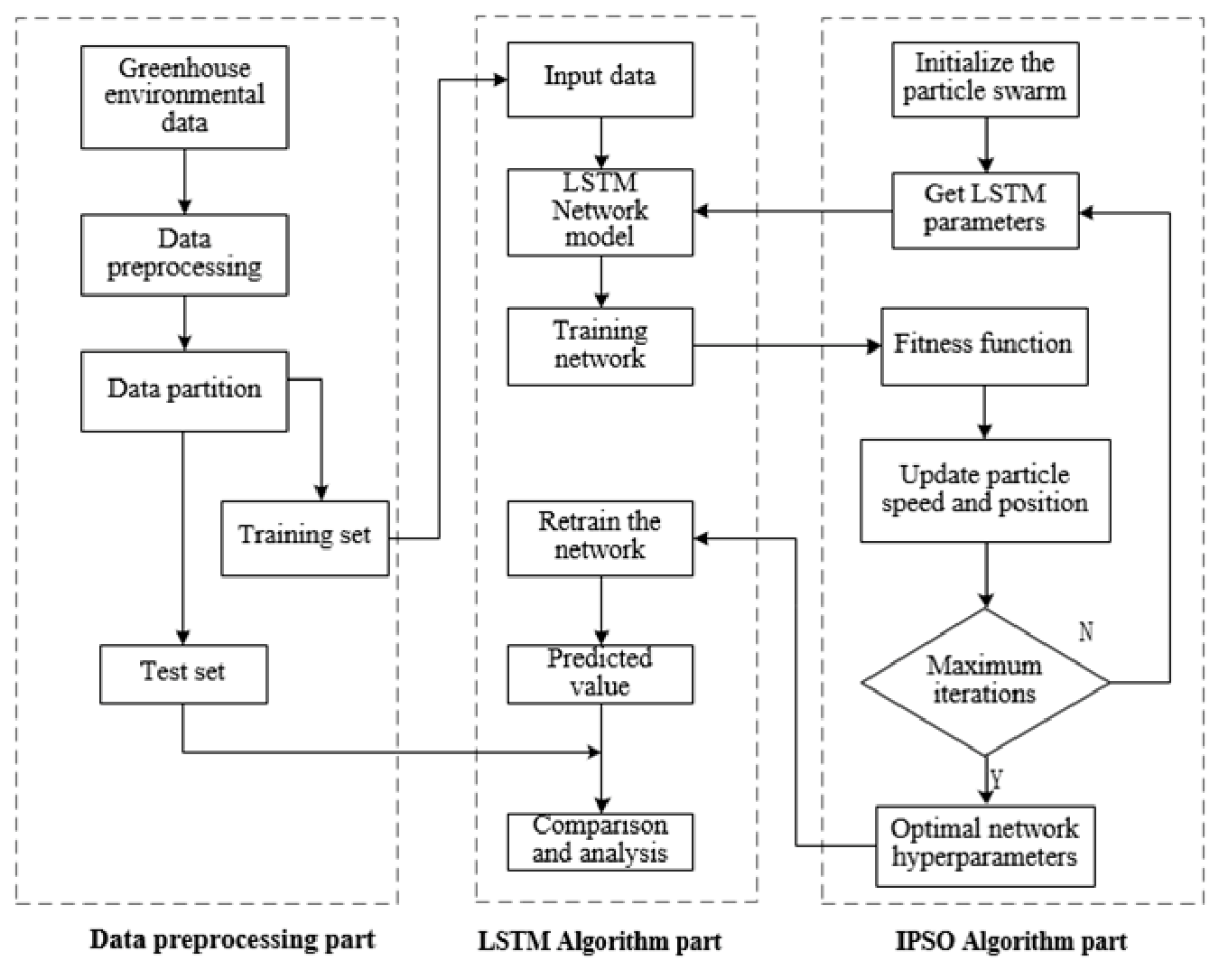
The Python (version 3.7) language was used to construct the combined model of IPSO-LSTM greenhouse temperature prediction. The open-source software Spyder was used to write the program, and different modules were implemented by calling NumPy, matplotlib, TensorFlow, and other modules. The collected greenhouse environment data was divided into training sets and testing sets. The training set was used to train the model, while the testing set was used to evaluate the model’s prediction performance. The IPSO-LSTM flowchart is illustrated in Figure 4.

Model implementation approach:

• Data collection: Collected environmental data from inside the greenhouse, including temperature and humidity.
• Data preprocessing: Utilized modules such as pandas and NumPy in Python to handle missing values and filter out anomalies in the collected greenhouse environment data. Normalized the data after preprocessing.
• Sample data partitioning: Divided the data into training sets and testing sets.
• Parameter initialization: Initialized IPSO parameters and set the initial parameters of the LSTM model, including the number of input layers, hidden layer neurons, output layer neurons, iteration count, learning rate, and batch size.
• Optimization process: Defined the fitness function “f.” The IPSO algorithm compared the fitness value of each particle, updated the particles’ positions and velocities within a certain number of iterations to find the global optimal value, and updated the hyperparameters of the LSTM model.
• Model prediction: Incorporated the optimal hyperparameters into the IPSO-LSTM combined model for greenhouse environment prediction, compared and analyzed the predicted values with the actual values.
• Repeat predictions: Performed repeated predictions with the improved model and compared the predictive accuracy of each model.

2.5. Evaluation Metrics

To verify the prediction performance of the IPSO-LSTM model, mean absolute error (MAE) [27], mean absolute percentage error (MAPE) [28], root mean square error (RMSE) [29] and coefficient of determination (R²) [30] were used as evaluation indexes of the model.

(1)

Mae [31]:

$$MAE={\displaystyle \frac{1}{n}}{\displaystyle \sum _{i=1}^n\left|x_i-{\tilde{x}}_i\right|}$$

(15)

where $n$ represents the number of collected greenhouse data points, $x_i$ represents the actual values, and ${\tilde{x}}_i$ represents the predicted values. MAE has a range of [0, ∞]. It calculates the average of the absolute differences between the predicted and actual values, providing an overall measure of the model’s accuracy. When the value is 0, the predicted values match the actual values, indicating a perfect model.

(2)

Mape [32]:

$$MAPE={\displaystyle \frac{1}{n}}{\displaystyle {\sum }_{i=1}^n\left|\frac{{\tilde{x}}_i-x_i}{x_i}\right|}\times 100\%$$

(16)

where $n$ represents the number of collected greenhouse data points, $x_i$ represents the actual values, and ${\tilde{x}}_i$ represents the predicted values. The MAPE has a range of [0, ∞]. It computes the average percentage difference between the predicted and actual values, indicating the model’s relative accuracy. When the value is 0, the predicted values match the actual values, indicating a perfect model.

(3)

RMSE [33]:

$$RMSE=\sqrt{{\displaystyle \frac{{\displaystyle {\sum }_{i=1}^n{({\tilde{x}}_i-x_i)}^2}}{n}}}$$

(17)

where $n$ represents the number of collected greenhouse data points, $x_i$ represents the actual values, and ${\tilde{x}}_i$ represents the predicted values. RMSE is the square root of the MSE and measures the deviation between the actual values and the predicted values. It has a range of [0, ∞], and a smaller value indicates that the predicted values are closer to the actual values.

(4)

R² [34]:

$$R^2=1-{\displaystyle \frac{{\displaystyle {\sum }_{i=1}^n{(x_i-{\tilde{x}}_i)}^2}}{{\displaystyle {\sum }_{i=1}^n{(x_i-{\overline{x}}_i)}^2}}}$$

(18)

where $n$ represents the number of collected greenhouse data points, $x_i$ represents the actual values, ${\tilde{x}}_i$ represents the predicted values, and ${\overline{x}}_i$ represents the mean value. The R² measures the goodness-of-fit of the model. It has a range of [0, 1], and a value closer to 1 indicates better model performance. When the value is 1, it means the predicted values are equal to the actual values, indicating a perfect fit of the model to the data.

3. Results and Discussion

3.1. Data Collection and Preprocessing

3.1.1. Data Collection

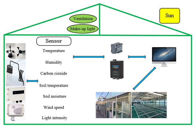
The greenhouse is classified as a Venlo-type glass greenhouse, located at the Dongfeng Campus of Zhengzhou University of Light Industry in Zhengzhou, Henan Province. The actual dimensions of the greenhouse are 16 m in length (north–south direction), 7.2 m in width (east–west direction), and 2.5 m in height. It is located at the East Campus of Zhengzhou University of Light Industry. The greenhouse environment data is collected using a data collection system, as shown in Figure 5, which consists of a PLC controller, actuators, and sensors [35]. For this experiment, only the temperature and humidity data inside the greenhouse are collected. The data collection process spans from March 2022 to May 2022, with data samples taken every hour. The data collection system operates continuously during the specified period and captures the temperature and humidity variations inside the greenhouse at regular intervals. The collected data is then stored in a structured format, ensuring proper organization and easy retrieval for further analysis.

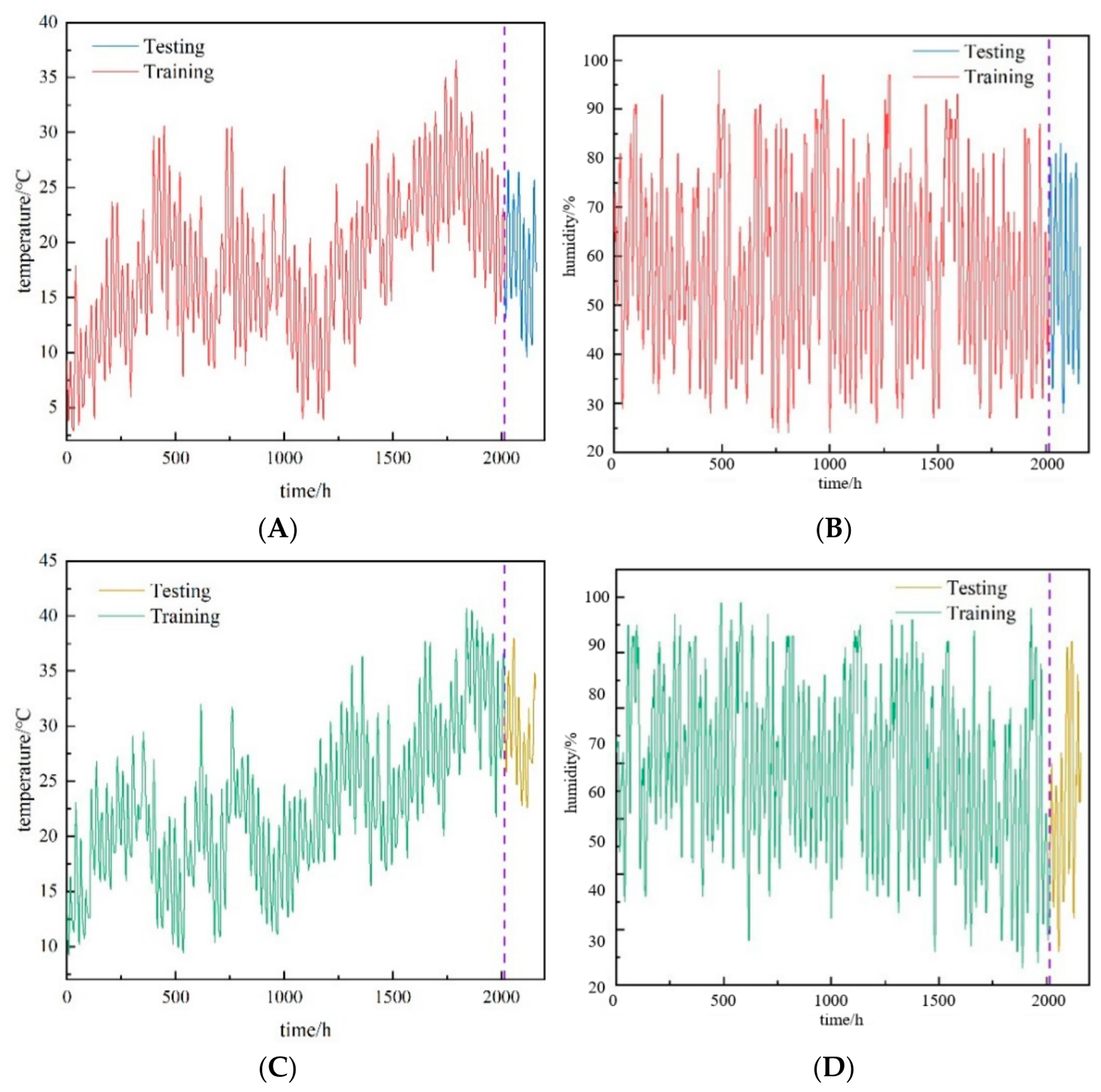
Figure 6 depicts the actual temperature and humidity data of tomatoes and cucumbers within the greenhouse collected by sensors. In Figure 6, the left side of the purple dashed line corresponds entirely to the training set, while the right side corresponds entirely to the test set. Figure 6A,B represent the temperature and humidity of the tomato growth environment, while Figure 6C,D illustrate the temperature and humidity of the cucumber growth environment. Figure 6A,C display the variation of indoor temperature in the greenhouse, which fluctuates mainly due to changes in the outside air temperature. The peaks represent the temperature at noon inside the greenhouse, while the valleys represent the temperature in the early morning. Figure 6B,D show the variation of indoor humidity in the greenhouse, which is influenced by soil evaporation and crop transpiration, and constantly changes. The rise in humidity is mainly caused by the irrigation of greenhouse crops. From the variation of temperature and humidity shown in Figure 6, it can be observed that both temperature and relative humidity exhibit non-linear patterns. The temperature and humidity vary from day to day, and their trends within the same period are also different.

The experiment divided the collected data into training sets and test sets, with the final 6 days (144 h) allocated for testing purposes. A comparison between the LSTM model and the PSO-LSTM prediction model was conducted to validate the superiority of the IPSO-LSTM model. The initial parameter settings for the LSTM prediction model were as follows: iteration times: 100; batch size: 128; artificial neurons: 50; fully connected layers: 20; and learning rate: 0.001. The summary of hyperparameters for the three prediction models is presented in

Table 3. Hyperparameters of three prediction models.

Forecasting Model	Forecasting Parameter	Iteration Times	Batch Size	Artificial Neuron	Fully Connected Layer	Learning Rate
LSTM	temperature	100	128	50	20	0.001
	humidity
PSO-LSTM	temperature	94	152	63	35	0.004
	humidity	67	114	31	23	0.006
IPSO-LSTM	temperature	98	139	65	6	0.008
	humidity	96	152	43	41	0.003

.

3.1.2. Exception Value Handling

During the data collection process, some data may be missing or contain outliers due to equipment issues, which can affect prediction accuracy. To address this, the NumPy module in Python was utilized to filter and remove outliers, fill in missing values, and transform the processed data. Specifically, missing values in the dataset are identified using the isnull function in the pandas library. For numerical features, missing values are filled in using the mean of the corresponding feature. The outlier identification formula is as follows:

$$O_x\left\{O_x<Q_1-1.5IQR;O_x>Q_3+1.5IQR\right\}$$

(19)

where $IQR$ is calculated as the difference between the 75th percentile (Q3) and the 25th percentile (Q1) of the data.

3.1.3. Data Standardization

The model used in this study has certain requirements for the input data and requires normalization and preprocessing of the data to scale different data features into the range [0, 1]. The formula is as follows:

$$\overline{X}={\displaystyle \frac{X-X_{\min }}{X_{\max }-X_{\min }}}$$

(20)

where $\overline{X}$ represents the standardized normalized data, with values ranging from [0, 1], $X$ represents the input data, $X_{\max }$ represents the maximum value of the input data, and $X_{\min }$ represents the minimum value of the input data.

3.2. Model Comparison

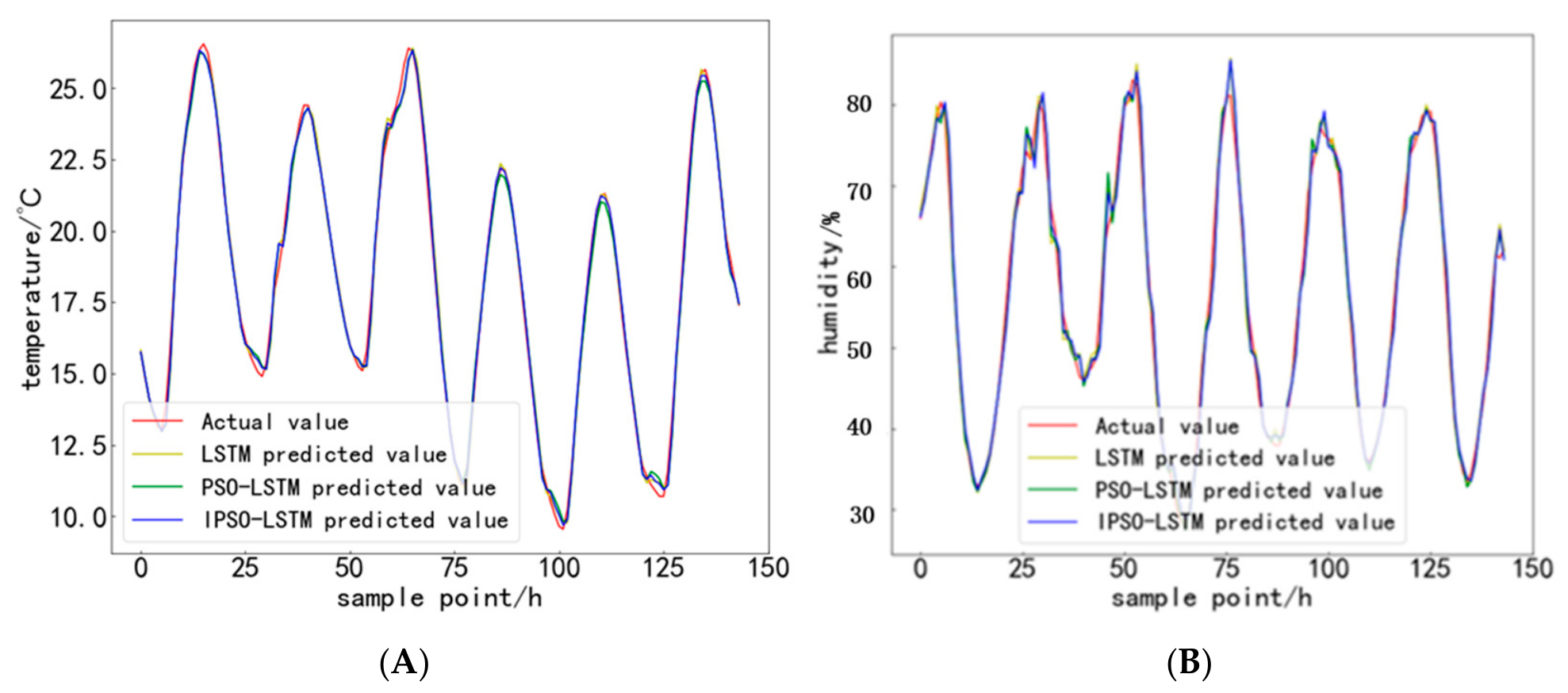
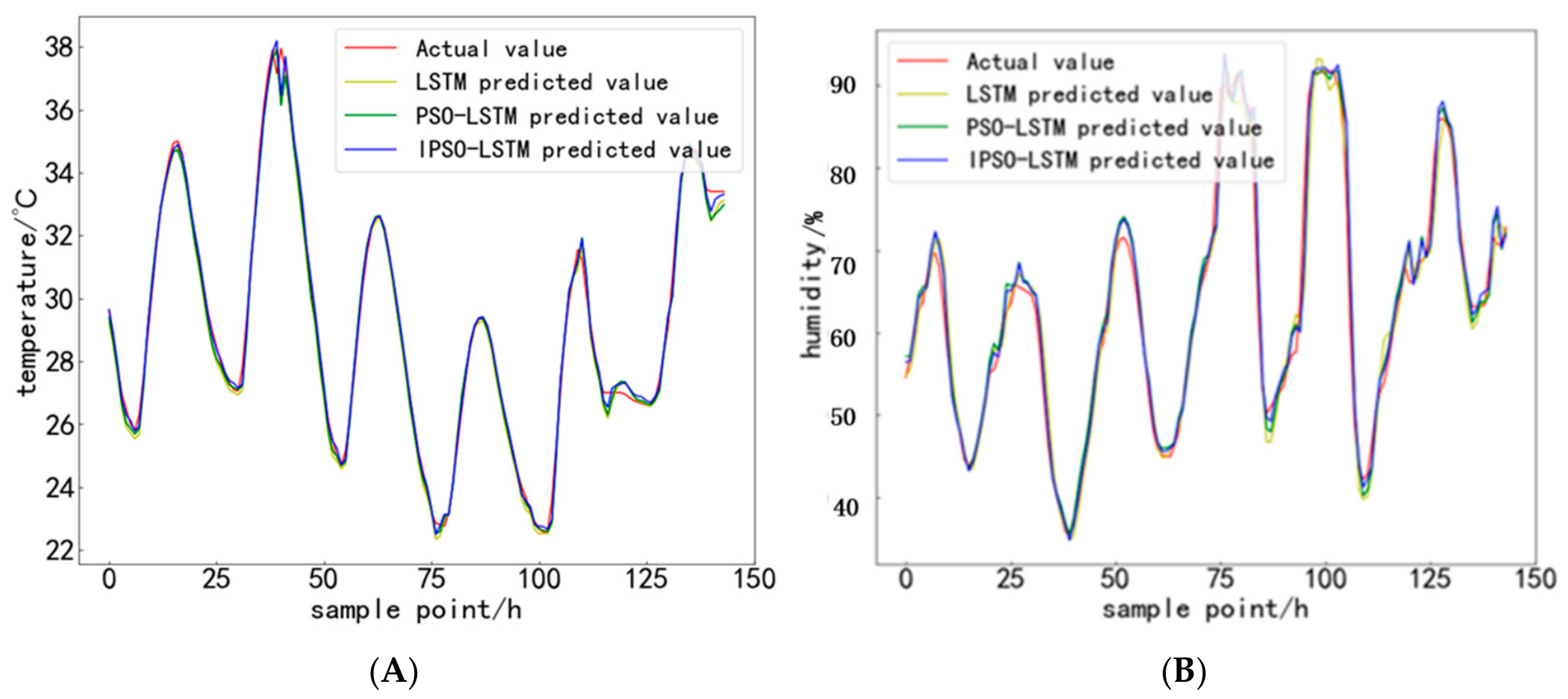
To validate the superiority of the IPSO-LSTM predictive model, we compared it with the PSO-LSTM and LSTM predictive models. For a concise presentation of the experimental results, we selected temperature and humidity data of tomatoes and cucumbers, respectively, for model training and prediction, and compared the predicted results with the real results. The parameter settings for the predictive models were kept consistent. Figure 7 and Figure 8 represent the predicted results for tomatoes and cucumbers, respectively. From Figure 7 and Figure 8, it can be observed that different data can lead to different predictive results. The predicted values of the three models generally exhibit similar trends to the actual values. However, at turning points, the predicted values of temperature and humidity exhibit significant deviations from the actual values, leading to lower predictive accuracy. This discrepancy is mainly attributed to the predictive model’s sensitivity to sudden changes or fluctuations in data, which can result in oscillations in the predicted values. In Figure 7A, the peaks and valleys represent the temperature values inside the tomato greenhouse during midday and nighttime, respectively, with a temperature difference of approximately 10 °C being maintained. Figure 7B illustrates the predicted humidity inside the tomato greenhouse. The predictions show larger deviations from the actual values around 25~50 h, mainly due to the model’s relatively weaker generalization ability to handle new data. After 50 h, the predicted values gradually stabilize and become closer to the actual values.

Figure 8A,B display the predictive results for temperature and humidity inside the cucumber greenhouse. The temperature predictions are notably more accurate than the humidity predictions. However, it is difficult to intuitively determine the superiority or inferiority of the predictive models from the visual inspection of the graphs.

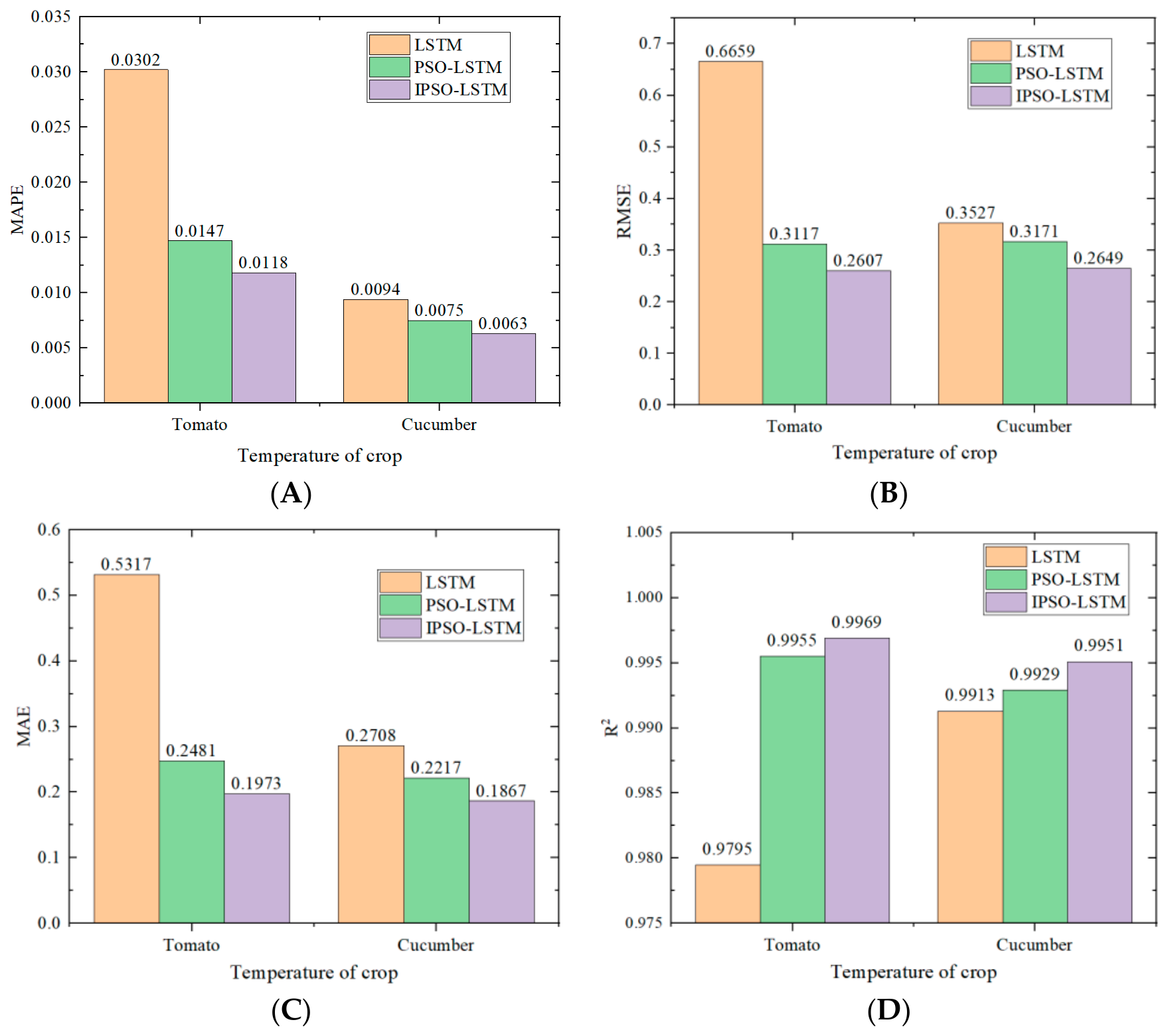
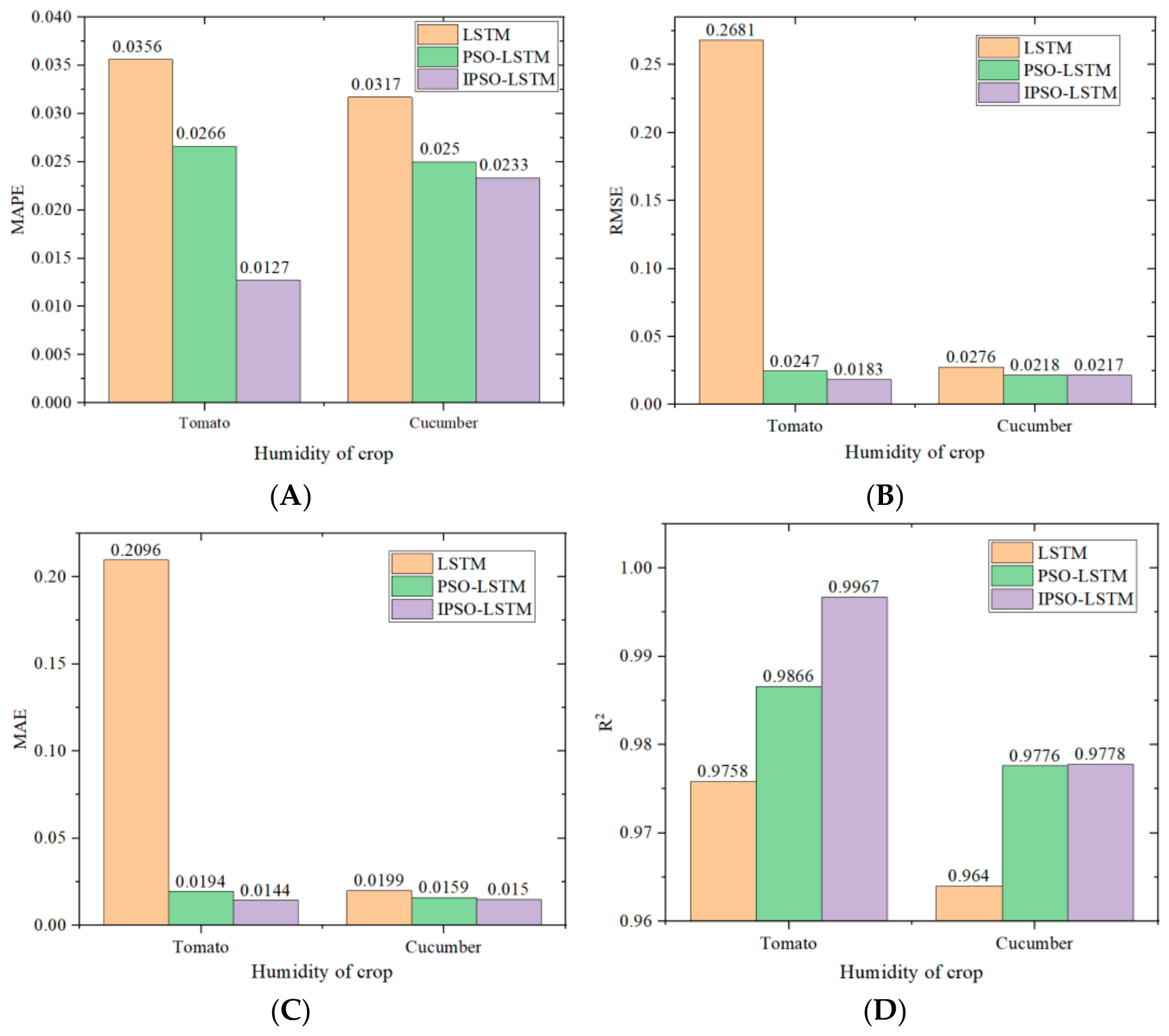
When making predictions, the superiority or inferiority of the prediction results from different prediction models is demonstrated through statistical metrics. Figure 9 and Figure 10 present the evaluation parameters (MAPE, RMSE, MAE, and R²) for the temperature and humidity prediction of the three models (IPSO-LSTM, PSO-LSTM, and LSTM) in both tomato and cucumber greenhouse environments. Smaller values of MAPE, RMSE, and MAE indicate smaller errors, and larger values of R² indicate better model fitting and, therefore, higher prediction accuracy of the model.

By comparing these evaluation parameters, the IPSO-LSTM model outperforms the PSO-LSTM and LSTM models, as indicated by its smaller MAPE, RMSE, and MAE values, and higher R² value. Specifically, in the temperature prediction for both tomato and cucumber greenhouses, the IPSO-LSTM model exhibits MAPE values less than 0.02, RMSE values less than 0.27, MAE values less than 0.2, and R² values greater than 0.9950, indicating its accurate temperature forecasting capability. In the humidity prediction for both crops, the IPSO-LSTM model demonstrates MAPE, RMSE, and MAE values less than 0.024, 0.022, and 0.015, respectively, with an R² value exceeding 0.9778. This shows the IPSO-LSTM model’s accuracy in humidity forecasting for greenhouse environments. It is worth noting that the R² value for humidity prediction in cucumber greenhouses is lower than that for tomato greenhouses, primarily due to the different predictive abilities of the model for distinct datasets. In conclusion, among the three prediction models, the IPSO-LSTM model exhibits significantly higher predictive accuracy than the PSO-LSTM and LSTM models, accurately reflecting the temperature variations within the greenhouse environment. Following the training of the models, the test statistical metrics for the two crops were obtained during the testing phase. The summaries of the evaluation metrics for the three prediction models in the testing phase are presented in

Table 4. Evaluation metrics for tomatoes during the testing phase.

Forecasting Model	Target	MAPE	RMSE	MAE	R2
LSTM	Temperature	0.0302	0.6659	0.5317	0.9795
	Humidity	0.0356	0.2681	0.2096	0.9758
PSO-LSTM	Temperature	0.0147	0.3117	0.2481	0.9955
	Humidity	0.0266	0.0247	0.0194	0.9866
IPSO-LSTM	Temperature	0.0118	0.2607	0.1973	0.9969
	Humidity	0.0127	0.0183	0.0144	0.9967

and

Table 5. Evaluation metrics for cucumbers during the testing phase.

Forecasting Model	Target	MAPE	RMSE	MAE	R2
LSTM	Temperature	0.0094	0.3527	0.2708	0.9913
	Humidity	0.0317	0.0276	0.0199	0.9640
PSO-LSTM	Temperature	0.0075	0.3171	0.2217	0.9929
	Humidity	0.0250	0.0218	0.0159	0.9776
IPSO-LSTM	Temperature	0.0063	0.2649	0.1867	0.9951
	Humidity	0.0233	0.0217	0.0150	0.9778

.

3.3. Prediction Results with Different Training Sample Volume

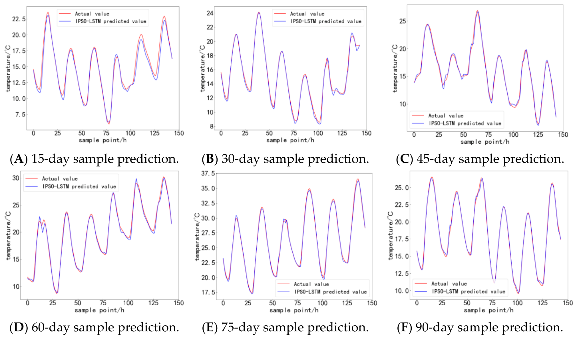
To investigate the impact of different training sample volumes on the IPSO-LSTM model’s prediction performance, we divided the collected temperature data from 90 days into six subsets: 15 days (A), 30 days (B), 45 days (C), 60 days (D), 75 days (E), and 90 days (F). Each subset was further split into training sets and testing sets, and we sequentially input them into the IPSO-LSTM model for training. The learning factors $c_1$ and $c_2$ were set to 1.5 and 1.5, respectively, while the random seed values $r_1$ and $r_2$ were set to 0.8 and 0.3, respectively. During the prediction process, the prediction results with different training sample sizes were compared, and the results are shown in Figure 11.

As shown in Figure 11, the prediction performance of the greenhouse model is improved with the increase in the number of training samples. Figure 11A shows that the predicted values consistently exhibit a certain deviation from the actual values, resulting in relatively large errors, but the model can simulate the general trend of the actual values. In Figure 11B, the model’s predicted values are relatively close to the actual values within the range of 0 to 100 h, but after 100 h, there is a larger discrepancy between the predicted and actual values. Figure 11C shows that during the peak and trough periods, there is considerable fluctuation in the deviation between predicted and actual values, and the model performs well on smooth data values. In Figure 11D, there are significant deviations in the predicted values from the actual values during the time intervals of 10–20 h and at the trough moments of 75 h, 100 h, and 125 h, while good predictive performance is observed at other times. Figure 11E,F demonstrate that the overall predictive performance is good, and the model can accurately predict the values even during peak and trough moments. To provide a more intuitive comparison of the effect of different training sample volumes on the model’s predictive performance, the evaluation parameters of the models are compared, as shown in Figure 12.

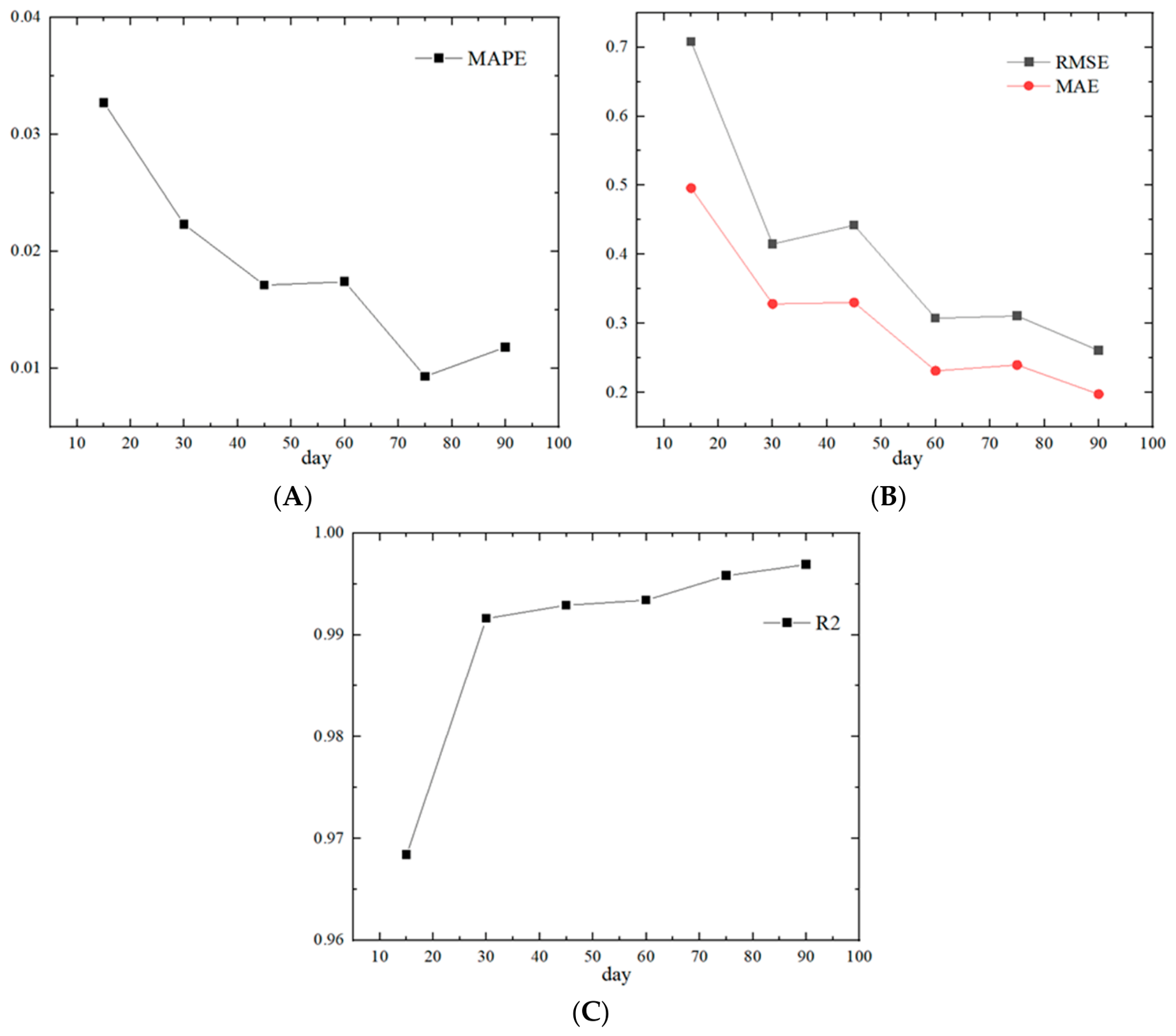
The comparison of evaluation parameters across different models under varying training sample sizes is shown in Figure 12. From Figure 12A, it can be observed that as the number of training samples increases, the value of MAPE gradually decreases, reaching its minimum at 75 days, and slightly increasing at 90 days. The MAPE decreases by 63.91% from 15 days to 90 days. Figure 12B shows that the evaluation parameters RMSE and MAE continuously decrease with the increase in training sample volume. From 15 days to 90 days, they decreased by 63.17% and 60.21%, respectively, signifying that the predictive performance of the model improved with an increase in the sample volume. The improvement is more significant in the early stages and becomes less pronounced in the later stages. Figure 12C shows that with the increase in training sample volume, R² increases from 0.9684 to 0.9969, showing a growth of 2.94%. The increase in R² is more apparent from 15 days to 30 days, and from 30 days to 90 days, it enters a slow growth phase. From the changes in the evaluation parameters, it can be observed that within a certain range of training sample volume, the predictive performance of the IPSO-LSTM model improves as the sample volume increases. However, when the data volume exceeds 90 days, the performance improvement of the model becomes marginal, while the training time of the model increases significantly.

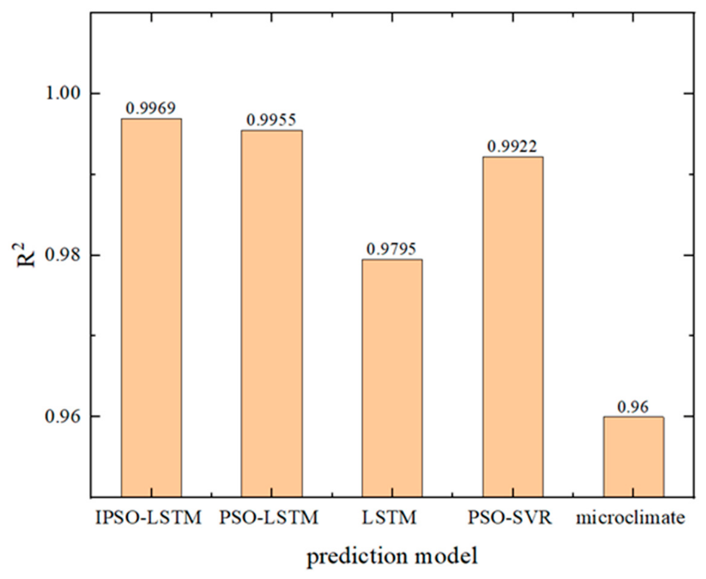
To compare the superiority of our proposed model in greenhouse environment prediction, we conducted a comparison with the models proposed in [23,36], as well as the models presented in previous sections. Figure 13 shows the comparison of evaluation parameters for different models. Compared to other prediction models, the IPSO-LSTM predictive model exhibits a significantly higher R² value of 0.9969. It is important to emphasize that a higher R² value indicates better predictive performance of the model. The comparison shows that the IPSO-LSTM predictive model proposed in this work exhibits superior predictive performance compared to the other models.

It is worth noting that the excellent prediction performance demonstrated within the 22–38 °C range primarily reflects the model’s high fidelity to the specific greenhouse microclimate under study. From a theoretical standpoint, the LSTM architecture itself is not inherently limited by specific temperature boundaries; it excels at extracting universal temporal patterns from sequential data. Therefore, the proposed IPSO-LSTM model possesses strong generalizability. While this study focuses on the typical temperature fluctuations of a controlled agricultural environment, the model architecture is fully capable of accommodating broader temperature ranges (e.g., −50 °C to 50 °C) if applied to other scenarios such as cold storage or extreme climate monitoring, provided that sufficient training data from those specific environments is available.

3.4. Implications for Greenhouse Management

Beyond statistical AI performance metrics, the predictive accuracy of the IPSO-LSTM model holds significant practical value for greenhouse environmental management. In modern agricultural practice, crop growth is highly sensitive to rapid fluctuations in temperature and humidity. For instance, achieving a temperature prediction RMSE of 0.2607 °C and a humidity MAPE of 0.0127 allows automatic climate control systems to preemptively adjust ventilation, shade nets, and heating mechanisms rather than relying on reactive control. This precise foresight effectively prevents the ‘thermal lag’ typical in large greenhouse structures, thereby protecting crops like tomatoes and cucumbers from microclimatic heat stress and condensation-induced fungal pathogens. Furthermore, preemptive dynamic adjustment helps avoid frequent, redundant equipment switching, directly optimizing the operational efficiency and energy consumption of greenhouse HVAC systems.

It should be noted that while modern deep learning architectures like Transformers and Attention-based networks excel in multi-variable non-linear modeling (e.g., Lee et al., 2025 [37]; Shi et al., 2024 [38]; Guo & Feng, 2024 [39]), the proposed IPSO-LSTM offers superior computational efficiency and lower parameter overhead, making it highly practical for lightweight edge deployment in greenhouse PLC or IoT control systems. Nevertheless, the current model implementation relies on a 90-day dataset; while sufficient for proof-of-concept demonstration, future practical implementation will necessitate multi-year data collection to ensure long-term seasonal robustness and mitigate potential overfitting risks.

4. Conclusions

An improved particle swarm optimization–long short-term memory (IPSO-LSTM) model was developed in this study to address the challenge of accurate greenhouse temperature and humidity prediction under non-linear, time-varying environmental conditions. A linearly decreasing inertia weight was integrated into the standard particle swarm optimization algorithm to automate the hyperparameter tuning of the LSTM network. The model was validated using 90-day hourly data collected from a Venlo-type glass greenhouse. For tomato cultivation scenarios, the coefficient of determination ($R^2$) reached 0.9969 for temperature prediction and 0.9967 for humidity prediction, with mean absolute percentage errors (MAPE) as low as 0.0118 and 0.0127, respectively. Consistent performance was also observed in cucumber growth environments, confirming the model’s generalization capability across crop types.

Further analysis revealed that expanding the training sample size from 15 days to 90 days reduced the MAPE, root mean square error (RMSE), and mean absolute error (MAE) by 63.91%, 63.17%, and 60.21%, respectively, while improving the $R^2$ by 2.94%. Compared with standard LSTM and conventional PSO-LSTM models, the proposed IPSO-LSTM achieved significantly higher prediction accuracy without relying on manual parameter tuning. The model provides a reliable technical basis for proactive greenhouse environmental regulation. Future work will focus on reducing computational overhead and incorporating additional environmental factors (e.g., CO₂ concentration, light intensity) to support more precise climate control.

However, it should be noted that the current study relies on a 90-day dataset; while sufficient for proof-of-concept demonstration, multi-year data collection is required in future studies to fully validate generalization across diverse seasons and mitigate potential overfitting risks. Furthermore, while modern architectures like Transformers and Attention-based networks excel in multi-variable modeling, IPSO-LSTM offers superior computational efficiency for practical PLC edge deployment. Future research will explore lightweight Transformer mechanisms to further evaluate long-term forecasting capabilities.

References

1. Ullah, I.; Fayaz, M.; Naveed, N.; Kim, D. ANN Based Learning to Kalman Filter Algorithm for Indoor Environment Prediction in Smart Greenhouse. IEEE Access 2020, 8, 159371–159388. [Google Scholar] [CrossRef] [Scilit]
2. Lin, D.Y.; Wei, R.H.; Xu, L.H. An Integrated Yield Prediction Model for Greenhouse Tomato. Agronomy 2019, 9, 873. [Google Scholar] [CrossRef] [Scilit]
3. Sahdev, R.K.; Kumar, M.; Dhingra, A.K. A comprehensive review of greenhouse shapes and its applications. Front. Energy 2019, 13, 427–438. [Google Scholar] [CrossRef] [Scilit]
4. Moon, T.; Son, J.E. Knowledge transfer for adapting pre-trained deep neural models to predict different greenhouse environments based on a low quantity of data. Comput. Electron. Agric. 2021, 185, 106136. [Google Scholar] [CrossRef] [Scilit]
5. Jung, D.-H.; Lee, T.S.; Kim, K.; Park, S.H. A Deep Learning Model to Predict Evapotranspiration and Relative Humidity for Moisture Control in Tomato Greenhouses. Agronomy 2022, 12, 2169. [Google Scholar] [CrossRef] [Scilit]
6. Jia, W.; Wei, Z. Short Term Prediction Model of Environmental Parameters in Typical Solar Greenhouse Based on Deep Learning Neural Network. Appl. Sci. 2022, 12, 12529. [Google Scholar] [CrossRef] [Scilit]
7. Arsenault, R.; Martel, J.-L.; Brunet, F.; Brissette, F.; Mai, J. Continuous streamflow prediction in ungauged basins: Long short-term memory neural networks clearly outperform traditional hydrological models. Hydrol. Earth Syst. Sci. 2023, 27, 139–157. [Google Scholar] [CrossRef] [Scilit]
8. Chen, Y.; Shi, G.; Jiang, H.; Zheng, T. Research on the Prediction of Insertion Resistance of Wheel Loader Based on PSO-LSTM. Appl. Sci. 2023, 13, 1372. [Google Scholar] [CrossRef] [Scilit]
9. Wang, J.; Xu, J.; Lu, Y.; Xie, T.; Peng, J.; Yang, F.; Ma, X. Prediction of molten pool temperature in laser solid forming based on PSO-LSTM. Front. Mater. 2023, 10, 1218222. [Google Scholar] [CrossRef] [Scilit]
10. Jiao, X.; Song, Y.; Kong, Y.; Tang, X.L. Volatility forecasting for crude oil based on text information and deep learning PSO-LSTM model. J. Forecast. 2022, 41, 933–944. [Google Scholar] [CrossRef] [Scilit]
11. Mu, G.; Liao, Z.; Li, J.; Qin, N.; Yang, Z. IPSO-LSTM hybrid model for predicting online public opinion trends in emergencies. PLoS ONE 2023, 18, e0292677. [Google Scholar] [CrossRef] [Scilit]
12. Huang, Q.; Wang, X. A Forecasting Model of Wind Power Based on IPSO-LSTM and Classified Fusion. Energies 2022, 15, 5531. [Google Scholar] [CrossRef] [Scilit]
13. Khatir, A.; Capozucca, R.; Khatir, S.; Magagnini, E.; Benaissa, B.; Le Thanh, C.; Wahab, M.A. A new hybrid PSO-YUKI for double cracks identification in CFRP cantilever beam. Compos. Struct. 2023, 311, 116803. [Google Scholar] [CrossRef] [Scilit]
14. Khatir, A.; Capozucca, R.; Khatir, S.; Magagnini, E.; Cuong-Le, T. Enhancing Damage Detection Using Reptile Search Algorithm-Optimized Neural Network and Frequency Response Function. J. Vib. Eng. Technol. 2025, 13, 88. [Google Scholar] [CrossRef] [Scilit]
15. Khatir, A.; Capozucca, R.; Khatir, S.; Magagnini, E. Vibration-based crack prediction on a beam model using hybrid butterfly optimization algorithm with artificial neural network. Front. Struct. Civ. Eng. 2022, 16, 976–989. [Google Scholar] [CrossRef] [Scilit]
16. Escamilla-Garcia, A.; Soto-Zarazua, G.M.; Toledano-Ayala, M.; Rivas-Araiza, E.; Gastélum-Barrios, A. Applications of Artificial Neural Networks in Greenhouse Technology and Overview for Smart Agriculture Development. Appl. Sci. 2020, 10, 3835. [Google Scholar] [CrossRef] [Scilit]
17. Liu, Y.; Li, D.; Wan, S.; Wang, F.; Dou, W.; Xu, X.; Li, S.; Ma, R.; Qi, L. A long short-term memory-based model for greenhouse climate prediction. Int. J. Intell. Syst. 2022, 37, 135–151. [Google Scholar] [CrossRef] [Scilit]
18. Ullah, I.; Fayaz, M.; Aman, M.; Kim, D. Toward Autonomous Farming-A Novel Scheme Based on Learning to Prediction and Optimization for Smart Greenhouse Environment Control. IEEE Internet Things J. 2022, 9, 25300–25323. [Google Scholar] [CrossRef] [Scilit]
19. Gao, M.; Wu, Q.; Li, J.; Wang, B.; Zhou, Z.; Liu, C.; Wang, D. Temperature prediction of solar greenhouse based on NARX regression neural network. Sci. Rep. 2023, 13, 1563. [Google Scholar] [CrossRef] [Scilit]
20. Mohammadi, B.; Mehdizadeh, S.; Ahmadi, F.; Linh, N.T.T.; Pham, Q.B. Developing hybrid time series and artificial intelligence models for estimating air temperatures. Stoch. Environ. Res. Risk Assess. 2021, 35, 1189–1204. [Google Scholar] [CrossRef] [Scilit]
21. Mohammadi, B. Modeling Various Drought Time Scales via a Merged Artificial Neural Network with a Firefly Algorithm. Hydrology 2023, 10, 58. [Google Scholar] [CrossRef] [Scilit]
22. Tran-Ngoc, H.; He, L.; Reynders, E.; Khatir, S.; Le-Xuan, T.; De Roeck, G.; Bui-Tien, T.; Wahab, M.A. An efficient approach to model updating for a multispan railway bridge using orthogonal diagonalization combined with improved particle swarm optimization. J. Sound. Vib. 2020, 476, 115315. [Google Scholar] [CrossRef] [Scilit]
23. Chen, X.Y.; Jiang, Z.H.; Tai, Q.L.; Shen, C.; Rao, Y.; Zhang, W. Construction of a photosynthetic rate prediction model for greenhouse strawberries with distributed regulation of light environment. Math. Biosci. Eng. 2022, 19, 12774–12791. [Google Scholar] [CrossRef] [Scilit]
24. Wang, D.; Tan, D.; Liu, L. Particle swarm optimization algorithm: An overview. Soft Comput. 2018, 22, 387–408. [Google Scholar] [CrossRef] [Scilit]
25. Yuan, P.; Lei, Z.; Zeng, Q.; Wu, Y.; Lu, Y.; Hu, C. Load forecasting of refrigerated display cabinet based on CEEMD-IPSO-LSTM combined model. Open Phys. 2021, 19, 360–374. [Google Scholar] [CrossRef] [Scilit]
26. Duc, T.T.; Ngoc, T.V.; Jongho, K. Improving the Accuracy of Dam Inflow Predictions Using a Long Short-Term Memory Network Coupled with Wavelet Transform and Predictor Selection. Mathematics 2021, 9, 551. [Google Scholar] [CrossRef] [Scilit]
27. Mendo, L. Estimation of a Probability with Guaranteed Normalized Mean Absolute Error. IEEE Commun. Lett. 2009, 13, 817–819. [Google Scholar] [CrossRef] [Scilit]
28. Khair, U.; Fahmi, H.; Al Hakim, S.; Rahim, R. Forecasting Error Calculation with Mean Absolute Deviation and Mean Absolute Percentage Error. In Proceedings of the International Conference on Information and Communication Technology (IconICT), Medan, Indonesia, 15 July–25 August 2017. [Google Scholar]
29. Soundiran, R.; Radhakrishnan, T.K.; Natarajan, S. Modeling of greenhouse agro-ecosystem using optimally designed bootstrapping artificial neural network. Neural Comput. Appl. 2019, 31, 7821–7836. [Google Scholar] [CrossRef] [Scilit]
30. Chicco, D.; Warrens, M.J.; Jurman, G. The coefficient of determination R-squared is more informative than SMAPE, MAE, MAPE, MSE and RMSE in regression analysis evaluation. PeerJ Comput. Sci. 2021, 7, e623. [Google Scholar] [CrossRef] [Scilit] [PubMed]
31. Qi, J.; Du, J.; Siniscalchi, S.M.; Ma, X.; Lee, C.-H. On Mean Absolute Error for Deep Neural Network Based Vector-to-Vector Regression. IEEE Signal Process. Lett. 2020, 27, 1485–1489. [Google Scholar] [CrossRef] [Scilit]
32. Wen, X.; Jaxa-Rozen, M.; Trutnevyte, E. Accuracy indicators for evaluating retrospective performance of energy system models. Appl. Energy 2022, 325, 119906. [Google Scholar] [CrossRef] [Scilit]
33. Karunasingha, D.S.K. Root mean square error or mean absolute error? Use their ratio as well. Inf. Sci. 2022, 585, 609–629. [Google Scholar] [CrossRef] [Scilit]
34. Piepho, H.-P. An adjusted coefficient of determination (R2) for generalized linear mixed models in one go. Biom. J. 2023, 65, e2200290. [Google Scholar] [CrossRef] [Scilit]
35. Kochhar, A.; Kumar, N. Wireless sensor networks for greenhouses: An end-to-end review. Comput. Electron. Agric. 2019, 163, 104877. [Google Scholar] [CrossRef] [Scilit]
36. Singh, M.C.; Singh, J.P.; Singh, K.G. Development of a microclimate model for prediction of temperatures inside a naturally ventilated greenhouse under cucumber crop in soilless media. Comput. Electron. Agric. 2018, 154, 227–238. [Google Scholar] [CrossRef] [Scilit]
37. Lee, J.; Im, S.; Jeong, J.-S.; Lee, T.S.; Park, S.H.; Shin, C.; Ju, H.; Kim, H.-J. Learning hidden relationship between environment and control variables for direct control of automated greenhouse using Transformer-based model. Comput. Electron. Agric. 2025, 235, 110335. [Google Scholar] [CrossRef] [Scilit]
38. Shi, D.; Yuan, P.; Liang, L.; Gao, L.; Li, M.; Diao, M. Integration of deep learning and sparrow search algorithms to optimize greenhouse microclimate prediction for seedling environment suitability. Agronomy 2024, 14, 254. [Google Scholar] [CrossRef] [Scilit]
39. Guo, Z.; Feng, L. Multi-step prediction of greenhouse temperature and humidity based on temporal position attention LSTM. Stoch. Environ. Res. Risk Assess. 2024, 38, 4907–4934. [Google Scholar] [CrossRef] [Scilit]
Figure 1. Study flow chart.
Agriengineering 08 00351 g001
Figure 2. Comparison of PSO and IPSO fitness curves.
Agriengineering 08 00351 g002
Figure 3. LSTM structure.
Agriengineering 08 00351 g003
Figure 4. Flow chart of IPSO-LSTM.
Agriengineering 08 00351 g004
Figure 5. Data collection and control system.
Agriengineering 08 00351 g005
Figure 6. Temperature and humidity data of tomato and cucumber in greenhouse: (A) Tomato greenhouse temperature; (B) Tomato greenhouse humidity; (C) Cucumber greenhouse temperature; (D) Cucumber greenhouse humidity. The purple dashed line separates the training set (left) and the testing set (right).
Agriengineering 08 00351 g006
Figure 7. Comparison of tomato temperature and humidity prediction. (A) Temperature prediction comparison; (B) Humidity prediction comparison.
Agriengineering 08 00351 g007
Figure 8. Comparison of cucumber temperature and humidity prediction. (A) Temperature prediction comparison; (B) Humidity prediction comparison.
Agriengineering 08 00351 g008
Figure 9. Comparison of temperature prediction evaluation parameters of different models. (A) MAPE values for temperature and humidity predictions. (B) RMSE values for temperature and humidity predictions. (C) MAE values for temperature and humidity predictions. (D) R2 values for temperature and humidity predictions.
Agriengineering 08 00351 g009
Figure 10. Comparison of humidity prediction evaluation parameters of different models. (A) MAPE values for temperature and humidity prediction. (B) RMSE values for temperature and humidity predictions. (C) MAE values for temperature and humidity predictions. (D) R2 values for temperature and humidity predictions.
Agriengineering 08 00351 g010
Figure 11. Prediction comparison curve of different training sample volumes.
Agriengineering 08 00351 g011
Figure 12. Comparison diagram of evaluation parameters. (A) MAPE variation with increasing sample size. (B) RMSE and MAE variation with increasing sample size. (C) R2 variation with increasing sample size.
Agriengineering 08 00351 g012
Figure 13. Comparison of evaluation coefficient R2 of different models.
Agriengineering 08 00351 g013