AI-Based Hybrid Deep Learning for Multiscale Red Tilapia Weight-Range Classification Using UAV Imagery

Abstract

This study proposed an artificial intelligence framework for red tilapia weight-range classification from UAV-based aerial imagery using two hybrid deep learning models, namely Hybrid CNN-XGBoost and Hybrid EfficientNet-B0-XGBoost. Two image sizes were evaluated: 5 × 5 m images, which preserved the spatial context of the cage culture system, and 2 × 2 m images, which focused on areas with high fish aggregation density. For the 5 × 5 m images, Hybrid CNN-XGBoost achieved the highest performance, with a mean accuracy of 0.988 ± 0.008 (98.8%) at 20 tuning units, whereas Hybrid EfficientNet-B0-XGBoost achieved 0.977 ± 0.021 (97.7%) at 40 tuning units. In addition, Hybrid CNN-XGBoost exhibited a substantially shorter average computational workflow time per image (0.038 ± 0.001 s) than Hybrid EfficientNet-B0-XGBoost (65.007 ± 6.141 s). In contrast, under the 2 × 2 m image condition with limited spatial context, Hybrid EfficientNet-B0-XGBoost outperformed Hybrid CNN-XGBoost, achieving the highest mean accuracy of 0.900 ± 0.010 (90.0%) at 30 tuning units, compared with 0.850 ± 0.022 (85.0%) at 50 tuning units. These findings indicate that larger images improve classification accuracy by preserving spatial context, whereas EfficientNet-B0 enhances deep feature extraction capability and improves classification accuracy when spatial context is limited.

1. Introduction

Red tilapia is one of the most important aquaculture species and serves as a major source of food and protein worldwide [1,2]. In Thailand, red tilapia farming has become increasingly popular because of the fish’s red body coloration, meat quality, and high tolerance to culture conditions [3,4,5]. During the production cycle, growth monitoring and fish weight assessment are still primarily based on conventional sampling and manual weighing methods, which are labor-intensive and may negatively affect fish feeding behavior and health [6,7,8]. To address these limitations, image—based fish weight estimation and aquatic animal monitoring techniques integrated with machine learning (ML), deep learning (DL), and hybrid models have gained increasing attention because they can improve prediction accuracy, reduce operational risks, and enhance aquaculture management efficiency [9].

Previous studies have demonstrated the potential of ML, DL, and hybrid models for image analysis across various applications, including medical imaging [10,11], agriculture [12], fisheries and aquaculture applications related to aquatic animal classification and weight estimation. Konovalov et al. [13] applied a DL convolutional neural network (CNN) model for Asian seabass (Lates calcarifer) weight estimation, whereas Tengtrairat et al. [14] employed a mask recurrent-convolutional neural network (Mask R-CNN) to estimate the weight of Nile tilapia (Oreochromis niloticus) cultured under laboratory conditions. Hamzaoui et al. [15] used the ML model extreme gradient boosting (XGBoost) for image-based weight estimation of several fish species, including European bream (Abramis brama), roach (Rutilus rutilus), whitefish (Coregoninae), common perch (Perca fluviatilis), northern pike (Esox lucius), and delta smelt (Hypomesus olidus). Feng et al. [16] compared EfficientNet and residual network (ResNet) for koi fish feeding behavior classification and reported that EfficientNet-B0 achieved higher classification accuracy than ResNet with accuracies of 98.78% and 94.81%, respectively. Similarly, Taparhudee et al. [9] reported that hybrid CNN-XGBoost improved red tilapia weight-range prediction accuracy compared with standalone CNN and XGBoost models while requiring fewer training epochs. Zhou et al. [17] demonstrated that EfficientNet-B0 combined with a random vector functional link model (EfficientNetB0-TRVFL) achieved superior performance for underwater image classification across multiple datasets. In addition, Biswal et al. [18] developed DeepFishNet, a hybrid model integrating you only look once version 9 (YOLOv9) and CNN for real-time fish disease classification, whereas Córdova et al. [19] proposed a multistage image-based framework in which YOLOv8 combined with EfficientNet-B0 provided robust and accurate fish detection and weight estimation under real-world conditions.

However, image-based fish weight estimation in real aquaculture environments still faces important challenges related to image acquisition, particularly under conditions in which data collection is restricted by limited viewing areas, fish movement, water surface interference, and farm-scale operational constraints. To address these limitations, unmanned aerial vehicles (UAVs) have emerged as a promising approach for acquiring aerial imagery in aquaculture systems. UAV-based imaging has previously been applied in a wide range of monitoring and management applications because of its flexibility, rapid image acquisition capability, and ability to capture large spatial areas under real farming conditions. In a previous study, Taparhudee et al. [9] applied a hybrid CNN-XGBoost model and reported a mean classification accuracy of 76%; however, the influence of image scale and backbone architecture on red tilapia weight-range classification using UAV imagery remains insufficiently investigated. To address this limitation, the present study explored the use of EfficientNet-B0 as an alternative backbone architecture, which has previously demonstrated high effectiveness and suitability for image feature extraction [16,17,19]. EfficientNet-B0 was selected as the backbone architecture in the present study because previous studies have demonstrated that it can achieve classification performance comparable to or better than widely used architectures such as ResNet and densely connected convolutional network (DenseNet) while requiring fewer parameters and lower computational complexity. Tan and Le [20] reported that EfficientNet achieved superior accuracy–efficiency tradeoffs through compound scaling of network depth, width, and input resolution. Similarly, Feng et al. [16] demonstrated that EfficientNet-B0 outperformed ResNet in fish image classification applications. Therefore, EfficientNet-B0 was considered an appropriate backbone architecture for evaluating improvements in red tilapia weight-range classification performance. In addition, Taparhudee et al. [9] used 2 × 2 m images to emphasize target objects while reducing background noise and surrounding interference. Nevertheless, this approach may result in the loss of important spatial contextual information, including fish distribution patterns, density, and schooling behavior, all of which are associated with fish weight classification in aquaculture systems. Previous studies on ML and DL image classification have reported that image context, image size, and spatial resolution play important roles in model performance [20,21]. Larger images can improve spatial feature extraction by preserving broader contextual information [22]. For example, Quintana et al. [23] reported that multiscale approaches integrating multiple patch sizes and image resolutions improved model performance compared with single-scale approaches. Similarly, de Bem et al. [24] demonstrated that larger image patches significantly improved classification accuracy because they preserved more spatial contextual information between objects and their surrounding environments, whereas smaller patches often failed to capture sufficient spatial relationships. Chen et al. [25] further reported that image size and spatial resolution directly influence model accuracy, with performance depending on the optimal spatial scale. Images with low resolution or small size may lose important object details and contextual information, whereas excessively high-resolution images may increase complexity and introduce additional noise. Likewise, Ashraf et al. [26] reported that larger image regions improved model accuracy because broader spatial coverage enabled simultaneous learning of both local object features and surrounding spatial context, whereas smaller regions tended to preserve only localized information and reduce structural and contextual representation.

Therefore, the present study extended previous research by investigating the combined effects of UAV image size and backbone architecture on red tilapia weight-range classification. Specifically, 2 × 2 m and 5 × 5 m image patches were compared to evaluate the influence of spatial context on classification performance, while EfficientNet-B0 was incorporated into the hybrid framework to assess whether backbone enhancement could further improve model performance. It was hypothesized that larger image patches would better preserve spatial contextual information and multiscale features, thereby improving classification accuracy, whereas EfficientNet-B0 would provide superior feature extraction capability under conditions with limited spatial context.

2. Materials and Methods

2.1. Ethical Statement and UAV Flight Permission

All experimental procedures were conducted in strict accordance with the applicable guidelines and regulations. The research protocol was approved by the Kasetsart University Institutional Animal Care and Use Committee (certificate no. ACKU 68-FIS-032) under the project title “AI-driven real-time monitoring of red tilapia weight and feeding efficiency using hybrid DL models with aerial imagery”. Furthermore, the DJI Air 2S UAV (DJI 13 store authorized dealer Thailand Co., Ltd., Bangkok, Thailand) used in this study was certified by Thailand’s Office of the National Broadcasting and Telecommunications Commission (certificate no. T040465013010) for radiocommunication equipment registration, permitting its use for research and experimental purposes. The UAV was registered under identification number RA—11—25—2530.

2.2. Fish Weight and Water Quality

One day before each experiment, 20 fish were randomly sampled from each cage and individually weighed using a CST-CDR-3 digital balance (CST Instruments Thailand Ltd., Bangkok, Thailand) to obtain actual fish body weight data. All fish handling and weighing procedures followed the protocol described by Taparhudee et al. [9]. Water quality parameters, including dissolved oxygen (DO), water temperature (Temp), potential hydrogen (pH), transparency (Trans), total ammonia nitrogen (TAN), nitrite–nitrogen (NO⁻₂-N), and alkalinity (ALK), were also monitored during the study. DO and Temp were measured using a YSI DO system (YSI, Yellow Springs, OH, USA), whereas pH was determined using a YSI pH 10A Pen Tester (YSI, Yellow Springs, OH, USA). Trans was measured using a Secchi disc. TAN, NO⁻₂-N, and ALK concentrations were analyzed using a portable field spectrophotometer (Spectrokit; Marine Leader Co., Ltd., Bangkok, Thailand) to enable rapid on-site assessment of water quality conditions.

The measured fish weights were subsequently used to calculate the mean body weight, standard deviation, minimum weight, and maximum weight of each sampling period. These weight statistics were used as reference information for defining fish weight classes and assigning weight-class labels to the corresponding UAV image datasets used for model development. Because the study was conducted under commercial farming conditions, some overlap between adjacent weight classes occurred due to natural fish size heterogeneity within the commercial red tilapia population.

2.3. Unmanned Aerial Vehicle (UAV), Image Acquisition, and Image Processing

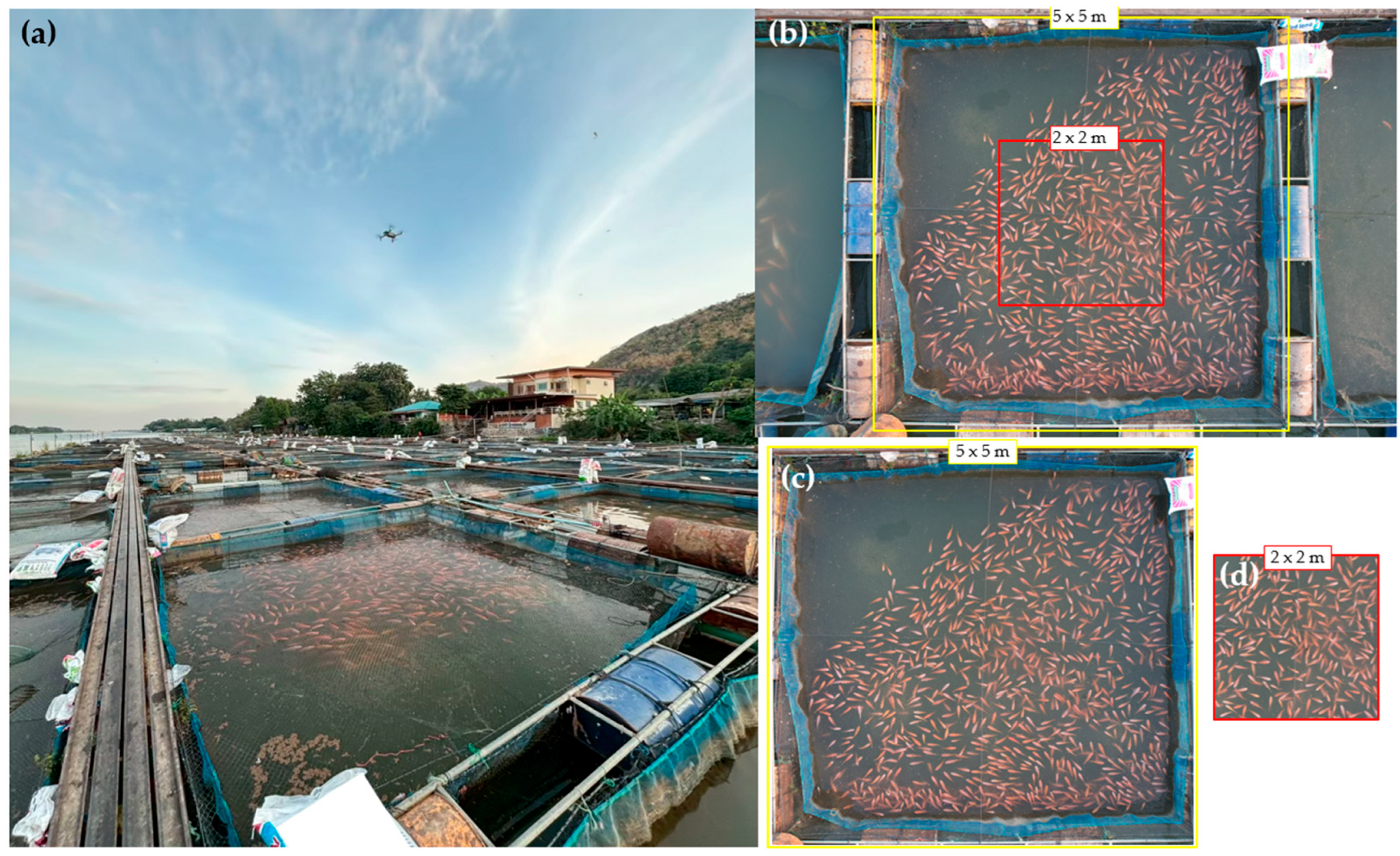
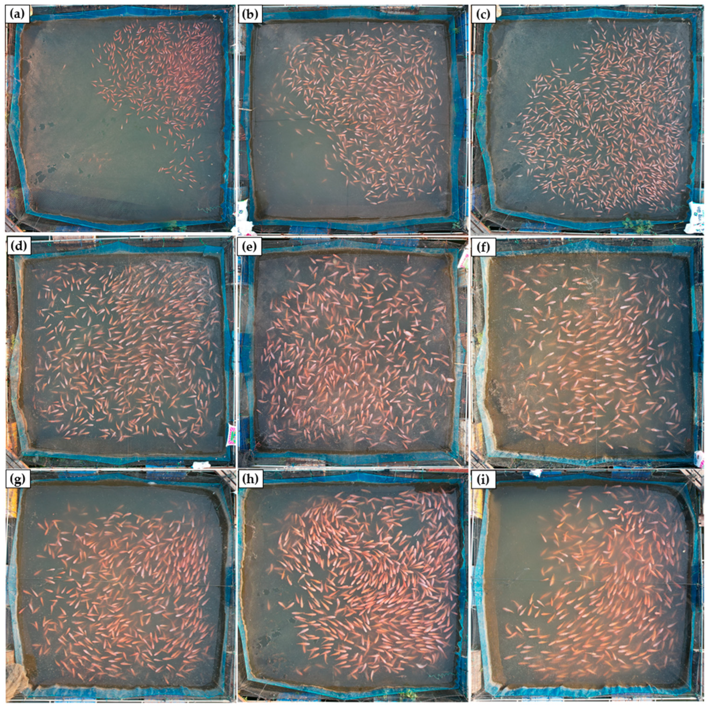
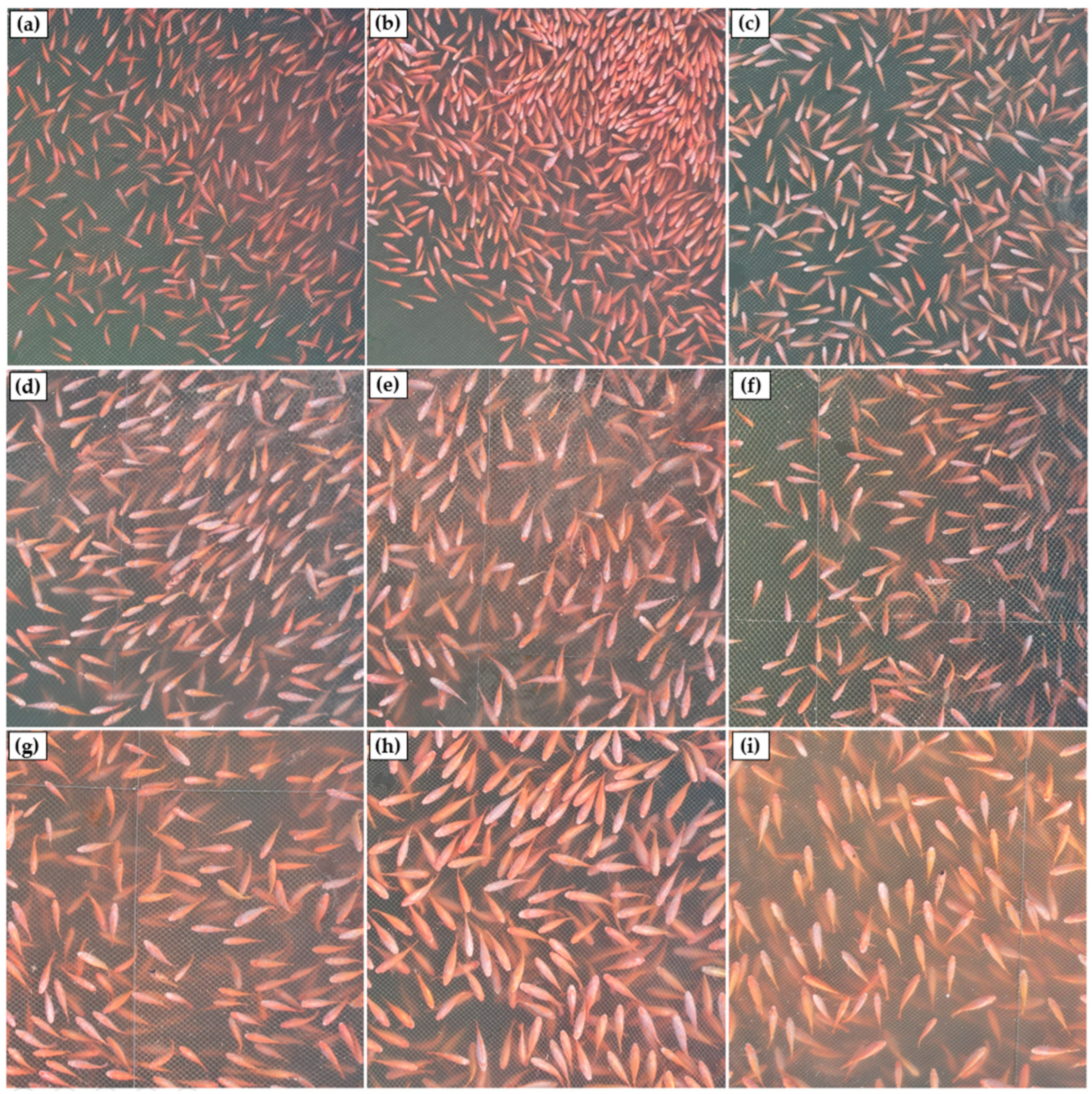
The UAV used in this study was a DJI Air 2S (Mavic), following the image acquisition protocol described by Taparhudee et al. [9]. The flight altitude from the UAV to the water surface above the fish cages was maintained at 3.5 m. Image acquisition was conducted across six fish cages throughout one production cycle from November 2025 to March 2026, with a total of nine flight sessions performed during the study period. A total of 2700 images were collected for image processing, corresponding to approximately 300 images per sampling session. The images used for model development and analysis were cropped into two image sizes, namely 5 × 5 m and 2 × 2 m (Figure 1).

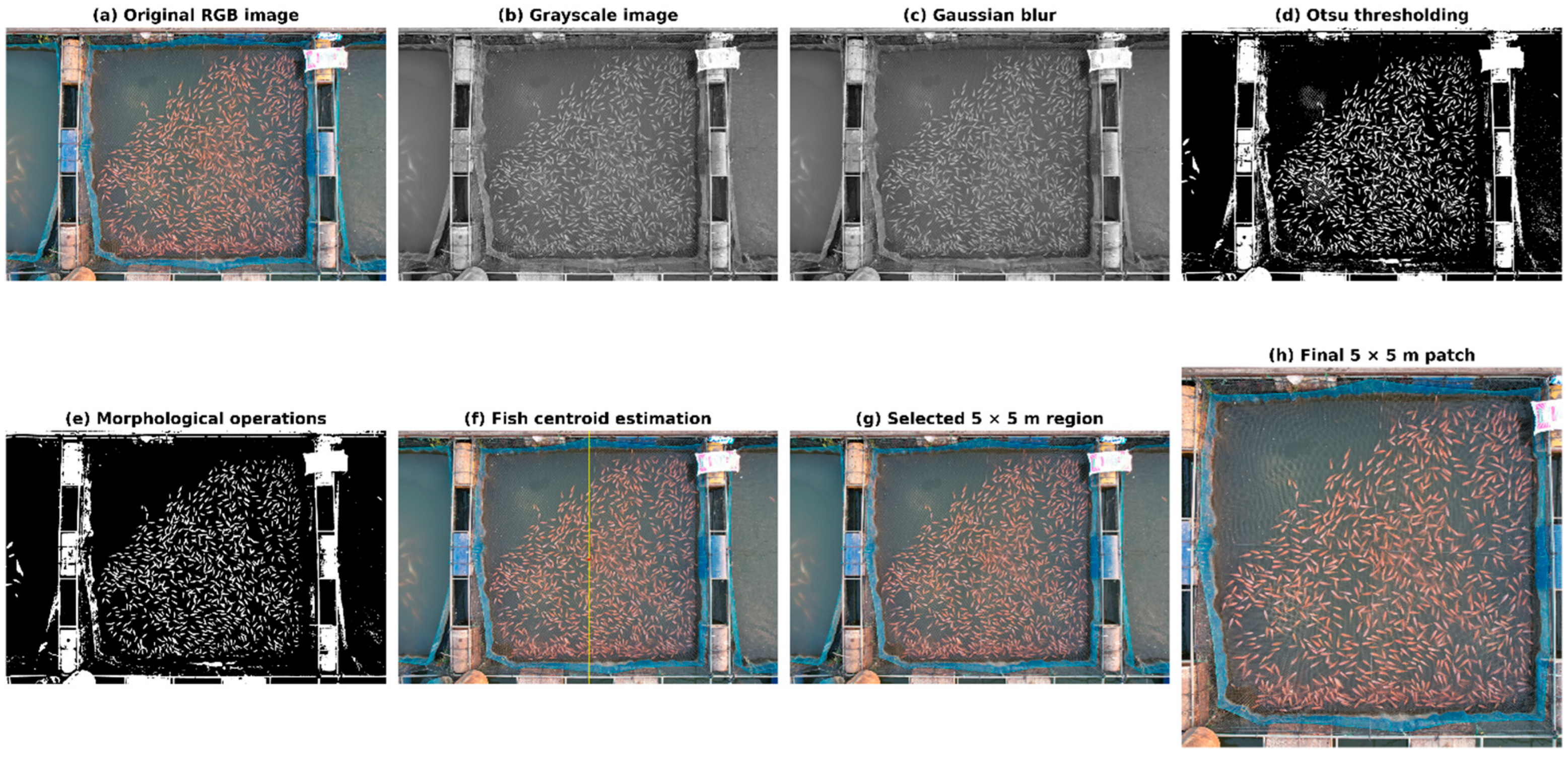
The generation of 5 × 5 m images was performed using a fish-centered 5 × 5 m patch extraction approach to obtain image patches that preserved the spatial context of fish distribution within the cage culture system (Figure 2). The process began with the original UAV-based RGB aerial image (Figure 2a), which was converted into a grayscale image to reduce image complexity (Figure 2b). Subsequently, Gaussian blur was applied to reduce image noise and improve object continuity within the image (Figure 2c). Otsu’s thresholding method was then used to separate fish objects from the water background (Figure 2d). Morphological operations, including opening and closing, were subsequently applied to reduce noise and improve the continuity and completeness of fish-object pixel groups (Figure 2e). Foreground pixels corresponding to fish objects were then used to calculate the fish centroid based on the average spatial coordinates of all foreground pixels (Figure 2f). A 5 × 5 m image patch was subsequently generated using the centroid position as the center of the cropping window (Figure 2g), while the cropping boundary was constrained to remain within the original image dimensions to avoid edge information loss. Finally, the extracted 5 × 5 m image patches preserved important spatial characteristics of the aquaculture system, including fish density, distribution patterns, and aggregation behavior, making them suitable as input data for subsequent hybrid DL model development (Figure 2h).

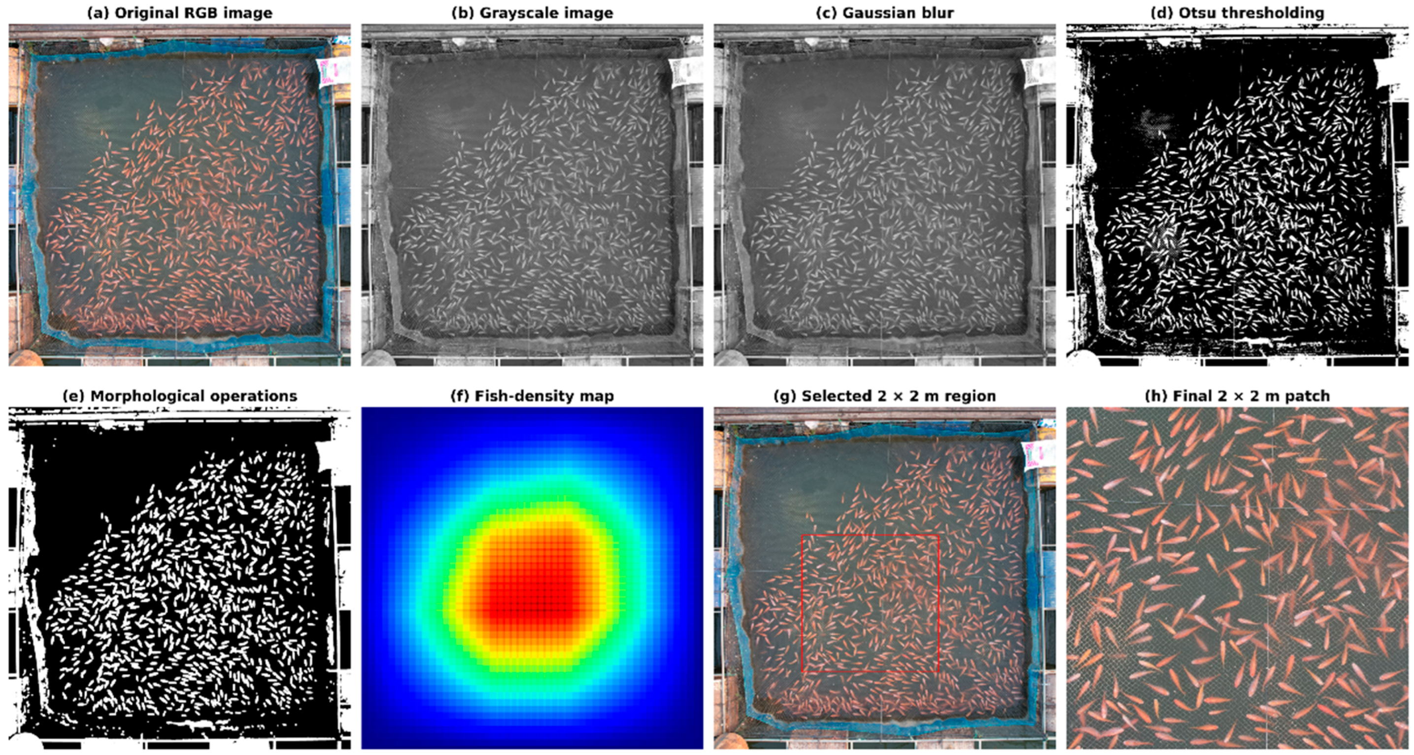
For the 2 × 2 m images, the previously generated 5 × 5 m image patches were subsequently processed using an automatic fish-density-based patch extraction approach to extract image patches from regions with the highest fish aggregation density (Figure 3). The process began with the previously generated 5 × 5 m image patch (Figure 3a), which was converted into a grayscale image to simplify image information (Figure 3b). Gaussian blur was subsequently applied to reduce image noise and improve image smoothness (Figure 3c). Otsu’s thresholding method was then used to separate fish objects from the background (Figure 3d), followed by morphological operations, including opening and dilation, to improve the continuity of fish-object pixel groups and reduce noise within the image (Figure 3e). A fish-density map was subsequently generated from the spatial distribution of foreground pixels to identify regions with the highest fish aggregation density (Figure 3f). A 2 × 2 m cropping window was then positioned over the region with the maximum density value (Figure 3g), and the resulting 2 × 2 m image patch was resized to 224 × 224 pixels for use as input data for the hybrid DL models (Figure 3h). This approach enabled the 2 × 2 m images to focus specifically on regions with high fish aggregation while minimizing the influence of background noise and surrounding cage interference. Consequently, the extracted patches were more suitable for capturing local fish aggregation features associated with fish weight-range classification in the subsequent modeling process.

2.4. CNN

CNN is a DL architecture specifically designed for processing spatially structured data, particularly images. A CNN consists of a multilayer architecture composed of an input layer, convolutional layers, activation layers, pooling or subsampling layers, and fully connected layers before the final output layer for classification or prediction tasks [9,27].

During the learning process, the convolutional layer extracts important image features using filters or kernels through convolution operations to learn object characteristics such as edges, textures, and shapes [28]. Activation layers, such as the rectified linear unit (ReLU), are subsequently applied to introduce nonlinearity into the network, enabling the model to learn more complex patterns and representations [29]. Pooling layers reduce the spatial dimensions of the feature maps while retaining the most informative features, thereby reducing the number of parameters, minimizing overfitting, and improving computational efficiency [30]. After multiple stages of feature extraction, the extracted features are passed to the fully connected layers to learn deeper feature relationships before being forwarded to the output layer for final classification. In general, CNN architectures consist of multiple stacked convolutional and pooling layers, enabling hierarchical representation learning from low-level to high-level image features [27,31,32]. The basic architecture of the CNN model used in this study is illustrated in Figure 4.

2.5. EfficientNet-B0

EfficientNet is a deep CNN architecture developed by Tan and Le [20] to improve learning efficiency while minimizing the number of parameters and computational cost, without compromising image classification accuracy. The core concept of this architecture is compound scaling, which systematically scales the network across three principal dimensions, including network depth, width, and image resolution, in a balanced manner. This approach enables the model to achieve efficient scaling while maintaining an appropriate balance between model complexity and classification performance [12,17,20]. Among the EfficientNet family (B0–B7), EfficientNet-B0 is considered the baseline model and is characterized by its relatively compact architecture and high computational efficiency. In the present study, EfficientNet-B0 was employed as a feature extractor to capture deep image features, particularly texture patterns and color characteristics, which are important factors for fish weight-range classification. The selection of EfficientNet-B0 was considered appropriate because the model can achieve classification performance comparable to that of larger architectures, such as ResNet-50, while requiring substantially fewer parameters and lower computational complexity [11,12,20].

The core architecture of EfficientNet-B0 comprises mobile inverted bottleneck convolution (MBConv) blocks, which were derived from the MobileNetV2 architecture. Each MBConv block consists of a 1 × 1 expansion convolution layer for increasing channel dimensions, a depthwise convolution layer for spatial feature extraction with low computational cost, and a 1 × 1 projection convolution layer for reducing channel dimensions back to a lower-dimensional representation. In addition, EfficientNet-B0 incorporates a squeeze-and-excitation (SE) module that performs channel attention by adaptively recalibrating the importance of each feature channel, thereby enhancing the model’s ability to emphasize informative image features [11]. Another important component of EfficientNet-B0 is its use of the Swish activation function instead of the conventional ReLU. The Swish function improves signal propagation continuity within the network and helps reduce information loss during the learning process. Consequently, EfficientNet-B0 demonstrates an improved capability to learn subtle image characteristics, such as variations in fish scale texture and body color patterns, which are important for fish weight-range classification under real aquaculture conditions.

Furthermore, EfficientNet-B0 employs the Swish activation function, which has been reported in previous studies to provide superior DL performance compared with the conventional ReLU activation function [33,34]. This improvement is primarily attributed to the ability of Swish to enhance gradient flow continuity throughout the network while reducing information loss during the learning process. As a result, the Swish activation function can improve feature learning capability, particularly for complex image patterns and subtle visual characteristics. The Swish activation function can be defined as Equation (1):

FSwish (x) = x/(1 + e^−βx)

(1)

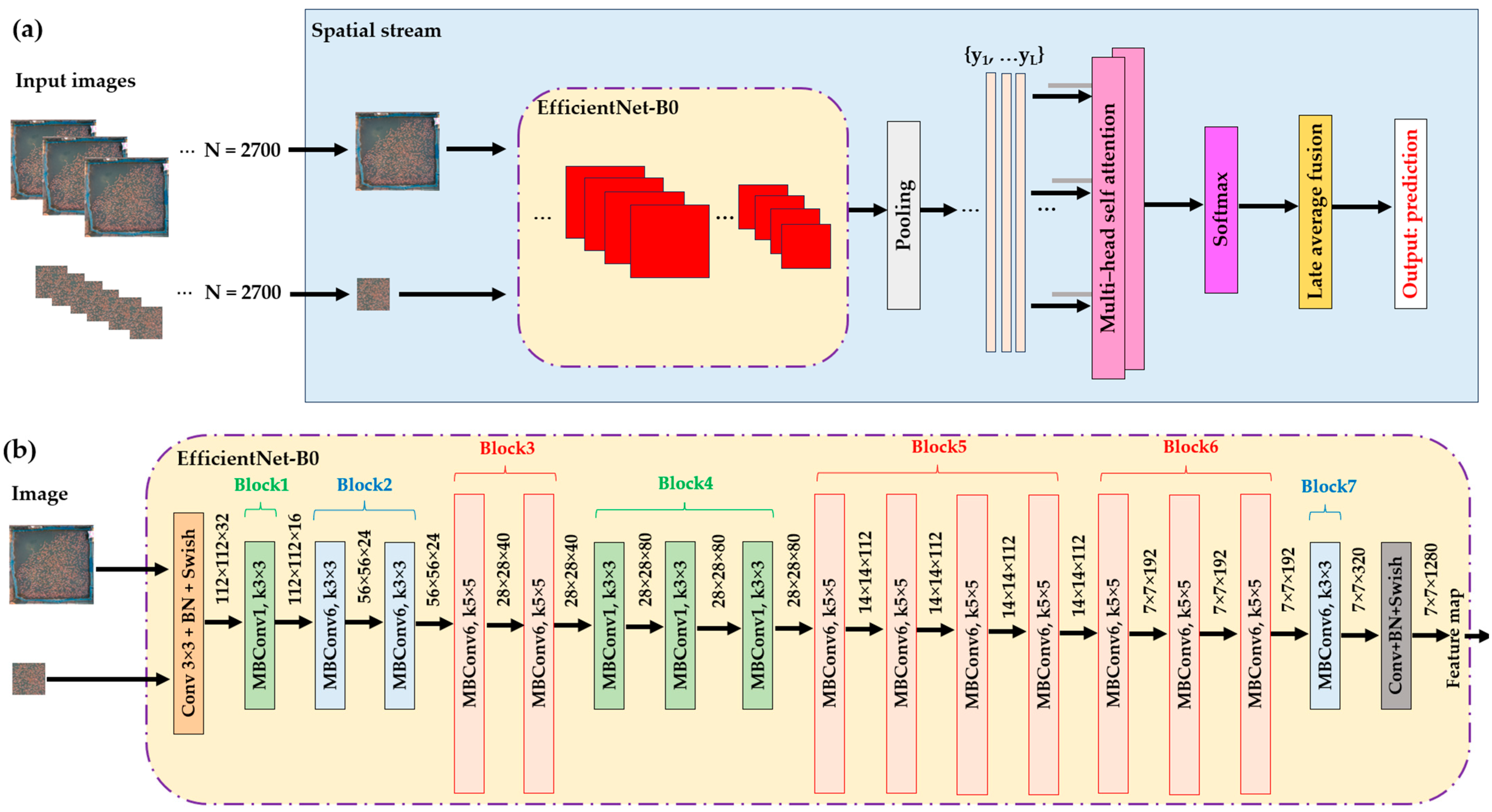
where FSwish (x) represents the Swish activation function, x is the input value, e denotes Euler’s number, and β is a trainable parameter that can be optimized during network training. This formulation enables smoother gradient propagation and improves learning stability within the network [34]. Owing to its combination of high classification accuracy, computational efficiency, and capability to process complex image data, EfficientNet-B0 was selected in the present study as the primary architecture for deep spatial feature extraction from red tilapia images. The basic EfficientNet-B0 architecture is shown in Figure 5.

In the present study, EfficientNet-B0 was selected as the primary model for deep feature extraction because of its high capability to balance classification accuracy and model complexity through the compound scaling approach, which systematically optimizes network depth, width, and image resolution. EfficientNet-B0 was initialized using pretrained ImageNet weights and modified by removing the fully connected layer to enable deep feature extraction from UAV-based red tilapia images. The extracted features represented important fish characteristics, including morphological features and coloration patterns, which are closely associated with fish weight estimation. Subsequently, principal component analysis (PCA) was applied to reduce feature dimensionality, eliminate redundant information, and decrease computational complexity before the ensemble learning process.

2.6. XGBoost

Extreme gradient boosting (XGBoost) is a boosting-based ensemble learning technique developed to improve model stability and predictive accuracy by sequentially constructing multiple decision trees, in which each subsequent tree learns from the errors generated by the previous trees. This iterative learning strategy enables the model to progressively improve prediction performance. A key advantage of XGBoost is its use of both first-order and second-order gradient information from the loss function, combined with regularization techniques to control model complexity, reduce overfitting, and improve learning efficiency when handling highly complex image data. Previous studies have demonstrated that XGBoost can improve classification performance and prediction accuracy in aquatic animal image analysis applications [9,15].

2.7. Model Development Pipeline

Hybrid CNN-XGBoost: The model development process consisted of two main stages: feature extraction using CNN and classification using XGBoost. Red tilapia images were resized to 64 × 64 pixels and passed through a CNN architecture composed of convolutional, pooling, and flatten layers to extract important image characteristics, including fish shape, texture, and body patterns. The flatten layer transformed the extracted image features into a one-dimensional feature vector representing the image information. The generated feature vectors were subsequently forwarded to the XGBoost classifier to categorize red tilapia into nine weight ranges through a gradient boosting decision tree mechanism.

Hybrid EfficientNet-B0-XGBoost: This model employed EfficientNet-B0 as the backbone architecture for deep feature extraction from red tilapia images. The training procedure involved a two-phase fine-tuning strategy. In phase 1, all backbone layers were frozen, and only the classifier head was trained to adapt the model to real fish image characteristics. In phase 2, all layers were unfrozen to enable EfficientNet-B0 to learn finer image-specific details of red tilapia, including body coloration patterns and morphological structures. After the global average pooling layer, a 1280-dimensional feature vector, corresponding to the final channel dimension of the original EfficientNet-B0 architecture [21], was extracted. Principal component analysis (PCA) was subsequently applied to reduce feature dimensionality from 1280 features to 128 principal components, thereby removing redundant information and retaining the most informative components before classification using XGBoost. Finally, XGBoost classified red tilapia into nine weight ranges using a boosting mechanism, thereby improving classification accuracy and enhancing model stability when handling highly variable image conditions obtained from real aquaculture environments.

In the model optimization process, training was initiated at 10 tuning units, namely epochs and n_estimators, and increased incrementally by 10 units until no further improvement in mean classification accuracy was observed across three consecutive tuning levels. To evaluate model stability and reduce the effects of stochastic variation during the learning process, all models at every tuning level were independently repeated five times, and the results are reported as the mean ± standard deviation.

For both Hybrid CNN-XGBoost and Hybrid EfficientNet-B0-XGBoost models, the image datasets were randomly partitioned into training (80%), validation (10%), and testing (10%) subsets using a stratified sampling strategy based on fish weight classes. Dataset partitioning was performed at the image level after image preprocessing and patch extraction, with a fixed random seed of 42. Because the partitioning was conducted at the image level rather than at the flight-session level, images originating from the same UAV flight session may have been distributed across the training, validation, and testing subsets. Therefore, a potential risk of similarity among samples originating from the same UAV flight session cannot be completely excluded. For the Hybrid EfficientNet-B0-XGBoost model, data augmentation, including random rotation, translation, brightness adjustment, shear transformation, zooming, and horizontal flipping, was applied exclusively to the training dataset to improve model generalization. The validation and testing datasets were not augmented and were retained as independent datasets for model evaluation.

2.8. Performance Evaluation

Model evaluation was performed using four primary metrics: accuracy, precision, recall, and F1 score. Accuracy reflects the ratio of correctly classified instances to the total number of samples. Precision indicates how many predicted positive outcomes were truly positive, whereas recall measures the proportion of actual positives that were accurately detected. F1 score, representing the harmonic mean of precision and recall, provides a balanced assessment of model performance between sensitivity and specificity.

All tasks related to data processing, image preprocessing, model development, training, evaluation, and visualization (Section 2.7 and Section 2.8) were performed using Python (version 3.11) within the Google Colaboratory cloud computing environment (Google LLC, Mountain View, CA, USA). For the Hybrid CNN-XGBoost model, the primary libraries included TensorFlow (version 2.19.0)/Keras (version 3.10.0) for CNN construction and training, OpenCV (version 4.11.0) for image processing, NumPy (version 2.1.3) for numerical computation, XGBoost (version 3.0.0) for gradient-boosting classification, Scikit-learn (version 1.6.1) for dataset partitioning and performance evaluation, and Matplotlib (version 3.10.0) and Seaborn Seaborn (version 0.13.2) for visualization and confusion matrix generation. For the Hybrid EfficientNet-B0-XGBoost model, TensorFlow/Keras was additionally used for transfer learning and two-phase fine-tuning of the EfficientNet-B0 architecture, while Scikit-learn was employed for label encoding, PCA, model evaluation, and data partitioning. Additional libraries included Pandas (version 2.2.3) for data management, OpenCV for image handling, NumPy for numerical operations, XGBoost for classification, and Matplotlib and Seaborn for graphical visualization and performance reporting.

2.9. Code Availability

The code used for image preprocessing, model development, training, and analysis is available from the corresponding authors upon reasonable request.

3. Results

3.1. Water Quality, Fish Weight, and Image Acquisition

The average water quality parameters throughout the experimental period, including DO, Temp, pH, TAN, NO⁻₂-N, ALK, and Trans, were 5.14 ± 0.52 mg/L, 26.58 ± 1.29 °C, 7.61 ± 0.06, 0.04 ± 0.04 mg/L, 0.01 ± 0.03 mg/L, 97.37 ± 7.94 mg/L, and 81.67 ± 10.71 cm, respectively. Based on the nine sampling periods conducted throughout the study, the average fish body weights were 92.00 ± 14.56, 137.88 ± 25.73, 178.41 ± 35.10, 241.54 ± 46.54, 359.27 ± 61.12, 449.41 ± 120.78, 595.17 ± 118.13, 652.78 ± 100.86, and 732.74 ± 101.27 g/fish, respectively. For UAV image acquisition, a total of nine flight sessions were conducted during the study period. Each flight session generated approximately 300 images for image processing, resulting in a total of 2700 images used for model development and analysis. The detailed experimental data are presented in

Table 1. Fish weight and image acquisition for each UAV flight session.

D/M/Y	Flight Session/Weight Class	Fish Weight (Mean ± SD) g/Fish	Fish Weight (Min–Max) g/Fish	Time	Number of Cages	Number of Images/Cages	Total Number of Images
30 November 2025	1	92.00 ± 14.56	62–129	7–8 a.m.	6	50	300
14 December 2025	2	137.88 ± 25.73	92–182	7–8 a.m.	6	50	300
28 December 2025	3	178.41 ± 35.10	112–262	7–8 a.m.	6	50	300
11 January 2026	4	241.54 ± 46.54	153–350	7–8 a.m.	6	50	300
25 January 2026	5	359.27 ± 61.12	270–460	7–8 a.m.	6	50	300
8 February 2026	6	449.41 ± 120.78	330–580	7–8 a.m.	6	50	300
22 February 2026	7	595.17 ± 118.13	476–748	7–8 a.m.	6	50	300
8 March 2026	8	652.78 ± 100.86	585–801	7–8 a.m.	6	50	300
22 March 2026	9	732.74 ± 101.27	655–906	7–8 a.m.	6	50	300

. Representative examples of the processed fish images for the 5 × 5 m and 2 × 2 m image sizes are shown in Figure 6 and Figure 7, respectively.

3.2. Model Performance and Processing Time

For the Hybrid CNN-XGBoost model using 5 × 5 m images, the highest model performance was obtained at 20 tuning units, with mean accuracy, precision, recall, and F1-score values of 0.988 ± 0.008, 0.988 ± 0.008, 0.988 ± 0.008, and 0.988 ± 0.008, respectively. The total computational workflow time of the model was 11.410 ± 0.447 s, whereas the average computational workflow time per image was 0.038 ± 0.001 s. In contrast, for the 2 × 2 m images, the highest performance of the Hybrid CNN-XGBoost model was achieved at 50 tuning units, with mean accuracy, precision, recall, and F1-score values of 0.850 ± 0.022, 0.856 ± 0.025, 0.850 ± 0.022, and 0.850 ± 0.022, respectively. The total computational workflow time was 19.616 ± 0.448 s, whereas the average computational workflow time per image was 0.065 ± 0.001 s.

In terms of backbone enhancement from CNN to Hybrid EfficientNet-B0-XGBoost, the results demonstrated that, for the 5 × 5 m images, the highest model performance was achieved at 40 tuning units, with mean accuracy, precision, recall, and F1-score values of 0.977 ± 0.021, 0.977 ± 0.021, 0.977 ± 0.021, and 0.977 ± 0.021, respectively. The total computational workflow time of the model was 19,502.000 ± 1842.333 s, whereas the average computational workflow time per image was 65.007 ± 6.141 s. For the 2 × 2 m images, the highest performance of the Hybrid EfficientNet-B0-XGBoost model was obtained at 30 tuning units, with mean accuracy, precision, recall, and F1-score values of 0.900 ± 0.010, 0.900 ± 0.010, 0.900 ± 0.010, and 0.898 ± 0.013, respectively. The total computational workflow time was 4254.800 ± 430.992 s, whereas the average computational workflow time per image was 14.183 ± 1.437 s. The detailed model performance and computational workflow time results are presented in

Table 2. Performance and computational workflow time of the Hybrid CNN-XGBoost and Hybrid EfficientNet-B0-XGBoost models for red tilapia weight-range classification using 5 × 5 m and 2 × 2 m UAV-based aerial images.

Image Size/Model	Tuning Units	Accuracy	Precision	Recall	F1	Total Computational Workflow Time (s)	Average Computational Workflow Time per Image (s)
5 × 5/Hybrid CNN-XGBoost	10	0.984 ± 0.005	0.984 ± 0.005	0.984 ± 0.005	0.984 ± 0.005	9.110 ± 1.342	0.030 ± 0.004
	20	0.988 ± 0.008	0.988 ± 0.008	0.988 ± 0.008	0.988 ± 0.008	11.410 ± 0.447	0.038 ± 0.001
	30	0.976 ± 0.009	0.976 ± 0.009	0.976 ± 0.009	0.976 ± 0.009	14.162 ± 0.457	0.047 ± 0.002
	40	0.970 ± 0.010	0.976 ± 0.008	0.970 ± 0.010	0.970 ± 0.010	16.688 ± 0.000	0.056 ± 0.000
	50	0.970 ± 0.016	0.970 ± 0.016	0.970 ± 0.016	0.970 ± 0.016	19.618 ± 0.448	0.065 ± 0.001
2 × 2/Hybrid CNN-XGBoost	10	0.610 ± 0.124	0.612 ± 0.130	0.610 ± 0.124	0.606 ± 0.125	8.892 ± 1.531	0.030 ± 0.005
	20	0.718 ± 0.103	0.720 ± 0.108	0.718 ± 0.103	0.712 ± 0.105	11.210 ± 0.000	0.037 ± 0.000
	30	0.826 ± 0.030	0.824 ± 0.029	0.820 ± 0.030	0.818 ± 0.033	14.110 ± 0.447	0.047 ± 0.001
	40	0.826 ± 0.015	0.832 ± 0.013	0.827 ± 0.015	0.826 ± 0.015	16.688 ± 0.000	0.056 ± 0.000
	50	0.850 ± 0.022	0.856 ± 0.025	0.850 ± 0.022	0.850 ± 0.022	19.616 ± 0.448	0.065 ± 0.001
	60	0.808 ± 0.015	0.816 ± 0.015	0.808 ± 0.015	0.808 ± 0.015	21.289 ± 1.164	0.071 ± 0.004
	70	0.820 ± 0.035	0.832 ± 0.030	0.820 ± 0.035	0.820 ± 0.041	24.275 ± 1.327	0.081 ± 0.004
	80	0.804 ± 0.033	0.822 ± 0.018	0.804 ± 0.033	0.826 ± 0.047	27.183 ± 2.348	0.091 ± 0.008
5 × 5/Hybrid EfficientNet-B0-XGBoost	10	0.920 ± 0.010	0.920 ± 0.010	0.920 ± 0.010	0.920 ± 0.010	6437.800 ± 516.427	21.459 ± 1.721
	20	0.940 ± 0.008	0.940 ± 0.008	0.940 ± 0.008	0.940 ± 0.008	11,381.500 ± 388.603	37.938 ± 1.295
	30	0.963 ± 0.021	0.963 ± 0.021	0.963 ± 0.021	0.963 ± 0.021	15,665.333 ± 1869.695	52.218 ± 6.226
	40	0.977 ± 0.021	0.977 ± 0.021	0.977 ± 0.021	0.977 ± 0.021	19,502.000 ± 1842.333	65.007 ± 6.141
	50	0.965 ± 0.006	0.963 ± 0.006	0.963 ± 0.006	0.963 ± 0.006	20,141.333 ± 3678.118	67.138 ± 12.260
	60	0.963 ± 0.006	0.963 ± 0.006	0.963 ± 0.006	0.963 ± 0.006	21,277.000 ± 72.505	70.923 ± 0.242
	70	0.973 ± 0.015	0.973 ± 0.015	0.973 ± 0.015	0.973 ± 0.015	26,466.333 ± 1742.844	88.221 ± 5.809
2 × 2/Hybrid EfficientNet-B0-XGBoost	10	0.786 ± 0.054	0.788 ± 0.050	0.786 ± 0.054	0.782 ± 0.052	2028.000 ± 986.705	6.760 ± 3.289
	20	0.758 ± 0.049	0.756 ± 0.049	0.758 ± 0.049	0.754 ± 0.050	2743.800 ± 1028.272	9.146 ± 3.428
	30	0.900 ± 0.010	0.900 ± 0.010	0.900 ± 0.010	0.898 ± 0.013	4254.800 ± 430.992	14.183 ± 1.437
	40	0.838 ± 0.082	0.838 ± 0.083	0.838 ± 0.082	0.836 ± 0.085	5629.400 ± 818.083	18.765 ± 2.727
	50	0.848 ± 0.054	0.848 ± 0.059	0.848 ± 0.054	0.844 ± 0.057	5748.000 ± 206.844	19.160 ± 0.689
	60	0.862 ± 0.068	0.866 ± 0.068	0.864 ± 0.067	0.864 ± 0.067	6061.400 ± 711.419	20.205 ± 2.371

Note: It should be noted that the reported total computational workflow time represents the complete computational time required for model development and evaluation. The total computational workflow time included all major computational stages associated with model development and evaluation. For the Hybrid CNN-XGBoost model, this included CNN training, feature extraction, XGBoost fitting, prediction, and model evaluation. For the Hybrid EfficientNet-B0-XGBoost model, the total computational workflow time additionally included the two-phase EfficientNet-B0 fine-tuning procedure, deep feature extraction, PCA dimensionality reduction, XGBoost fitting, prediction, and model evaluation. The reported average computational workflow time per image was calculated by dividing the total computational workflow time by the number of images included in each experimental condition. Therefore, the reported values should be interpreted as computational workflow metrics rather than the inference time of a fully trained model during practical deployment. Shaded rows and bold values indicate the best-performing (optimal) tuning units for each model and image patch size. These optimal configurations were subsequently used for the confusion matrix and class-wise accuracy analyses presented in Figure 8 and Figure 9.

.

For class-based classification accuracy, representative confusion matrices are shown in Figure 8, and the mean classification accuracies for each fish weight class are presented in Figure 9. For the Hybrid CNN-XGBoost model using 5 × 5 m images, the mean classification accuracies for Classes 1–9 were 98.000 ± 1.826, 100.000 ± 0.000, 99.333 ± 1.491, 96.667 ± 0.000, 97.333 ± 1.491, 100.000 ± 0.000, 98.000 ± 1.826, 94.667 ± 1.826, and 100.000 ± 0.000%, respectively. In contrast, for the 2 × 2 m images, the mean classification accuracies for Classes 1–9 were 92.667 ± 1.491, 98.000 ± 2.981, 86.667 ± 3.333, 67.333 ± 2.789, 66.667 ± 7.071, 88.667 ± 9.006, 90.000 ± 4.082, 86.000 ± 3.651, and 88.667 ± 5.055%, respectively. For the Hybrid EfficientNet-B0-XGBoost model using 5 × 5 m images, the mean classification accuracies for Classes 1–9 were 100.000 ± 0.000, 100.000 ± 0.000, 95.833 ± 3.191, 92.500 ± 9.574, 91.667 ± 4.303, 100.000 ± 0.000, 100.000 ± 0.000, 99.167 ± 1.667, and 100.000 ± 0.000%, respectively. Meanwhile, for the 2 × 2 m images, the mean classification accuracies for Classes 1–9 were 100.000 ± 0.000, 99.333 ± 1.491, 82.667 ± 4.346, 83.333 ± 4.082, 71.333 ± 7.303, 100.000 ± 0.000, 79.333 ± 5.447, 95.333 ± 2.981, and 96.667 ± 0.000%, respectively.

4. Discussion

4.1. Water Quality, Fish Weight, and Image Acquisition

The average values of all measured water quality parameters were within suitable ranges for red tilapia culture. DO remained above 3 mg/L, which is considered adequate for tilapia growth and survival [35]. Temp was maintained within the suitable range of 26–32 °C, whereas pH remained within the optimal range of 6.5–8.0. ALK values were within the recommended range of 50–400 mg/L [36]; TAN and NO⁻₂-N concentrations remained below 1 mg/L, which is considered safe for tilapia culture [37]. In addition, the average Trans value (81.67 ± 10.71 cm) showed no apparent negative effects on red tilapia feeding behavior or growth performance [9].

Beyond supporting fish growth and welfare, the favorable water quality conditions observed in the present study likely contributed to the quality and consistency of the UAV-derived image dataset used for model development. Adequate DO and low TAN levels are associated with normal feeding activity, growth performance, and behavioral patterns of tilapia [35,37]. Under such conditions, fish are more likely to exhibit consistent swimming and aggregation behaviors, which may improve fish visibility and detectability within UAV-based aerial images. Furthermore, the relatively high Trans observed during the study enhanced image clarity and facilitated fish observation from aerial imagery, consistent with the findings reported by Taparhudee et al. [9]. In contrast, deteriorated water quality conditions, such as low DO concentrations, elevated TAN levels, or reduced Trans, may alter fish behavior, reduce fish visibility, and increase image variability, potentially decreasing the effectiveness of image-based feature extraction and classification. Therefore, the favorable environmental conditions observed in this study likely contributed not only to fish production performance but also to the reliability and effectiveness of UAV-based fish weight-range classification.

For the fish weight, the observed minimum and maximum fish weights partially overlapped among adjacent weight classes. This overlap reflects the natural size heterogeneity commonly observed in commercial red tilapia production systems, where fish are not completely size-graded during the grow-out period. Consequently, the proposed AI-based classification framework was developed under realistic farming conditions rather than under strictly controlled size distributions.

For image acquisition, the UAV flight altitude of 3.5 m was sufficient to fully cover the 5 × 5 m cage area (Figure 1b), allowing the captured imagery to maintain an appropriate ground sample distance (GSD) for image analysis and fish feature extraction [38,39,40]. In addition, image collection was conducted during the morning prior to feeding, which helped minimize the effects of water-surface glare and coincided with periods when red tilapia tended to aggregate closer to the water surface. These conditions improved the visibility of fish within the images and enhanced the effectiveness of fish weight-range detection and classification [9].

4.2. Effects of Image Size on Model Performance

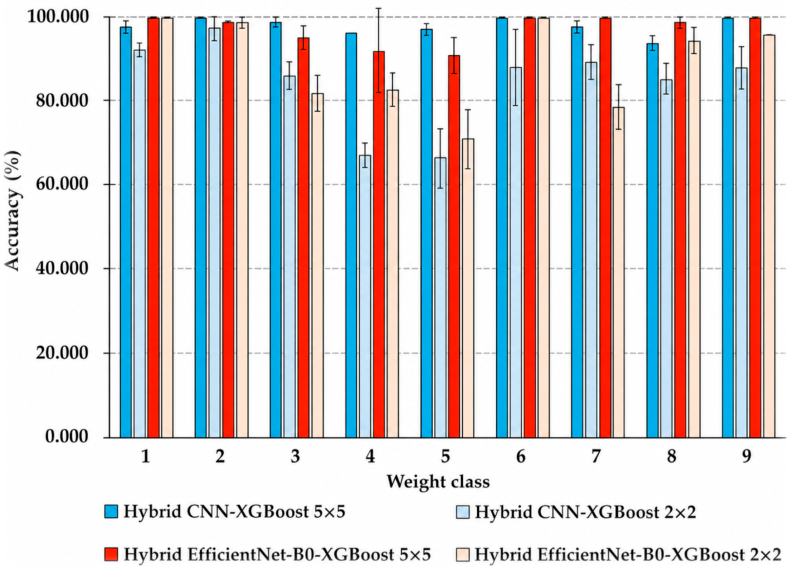
The results demonstrated that the use of 5 × 5 m images provided higher fish weight-range classification performance than 2 × 2 m images across all models evaluated in this study. This improvement can be attributed to the ability of larger images to more effectively preserve the spatial context of the aquaculture system, including fish distribution patterns, stocking density, and aggregation behavior, all of which represent important information for DL-based image analysis. This is particularly relevant for UAV-based image analysis, where image coverage area and spatial resolution directly influence feature extraction capability and object classification accuracy [25]. The findings of the present study are consistent with those of several previous studies. Quintana et al. [23] reported that the use of larger image patches or multiscale image information significantly improved model performance. Similarly, de Bem et al. [24] demonstrated that larger image patches preserved more spatial contextual information, thereby enabling the model to better learn the relationships between objects and their surrounding environments. Ashraf et al. [26] further reported that broader image regions enhanced the ability of the model to simultaneously learn both local object features and global spatial features, whereas smaller image regions often resulted in the loss of structural and contextual information, thereby reducing classification performance. In the present study, the 5 × 5 m images capture both individual fish characteristics and collective fish aggregation patterns within the cage culture system. These image characteristics may better reflect the relationships among fish size, stocking density, and swimming behavior within the farming environment. In contrast, the 2 × 2 m images primarily focused on regions with high fish aggregation density, which may limit the available spatial context and reduce the ability of the models to learn broader system-level spatial relationships.

4.3. Effects of Backbone Enhancement from CNN to EfficientNet-B0

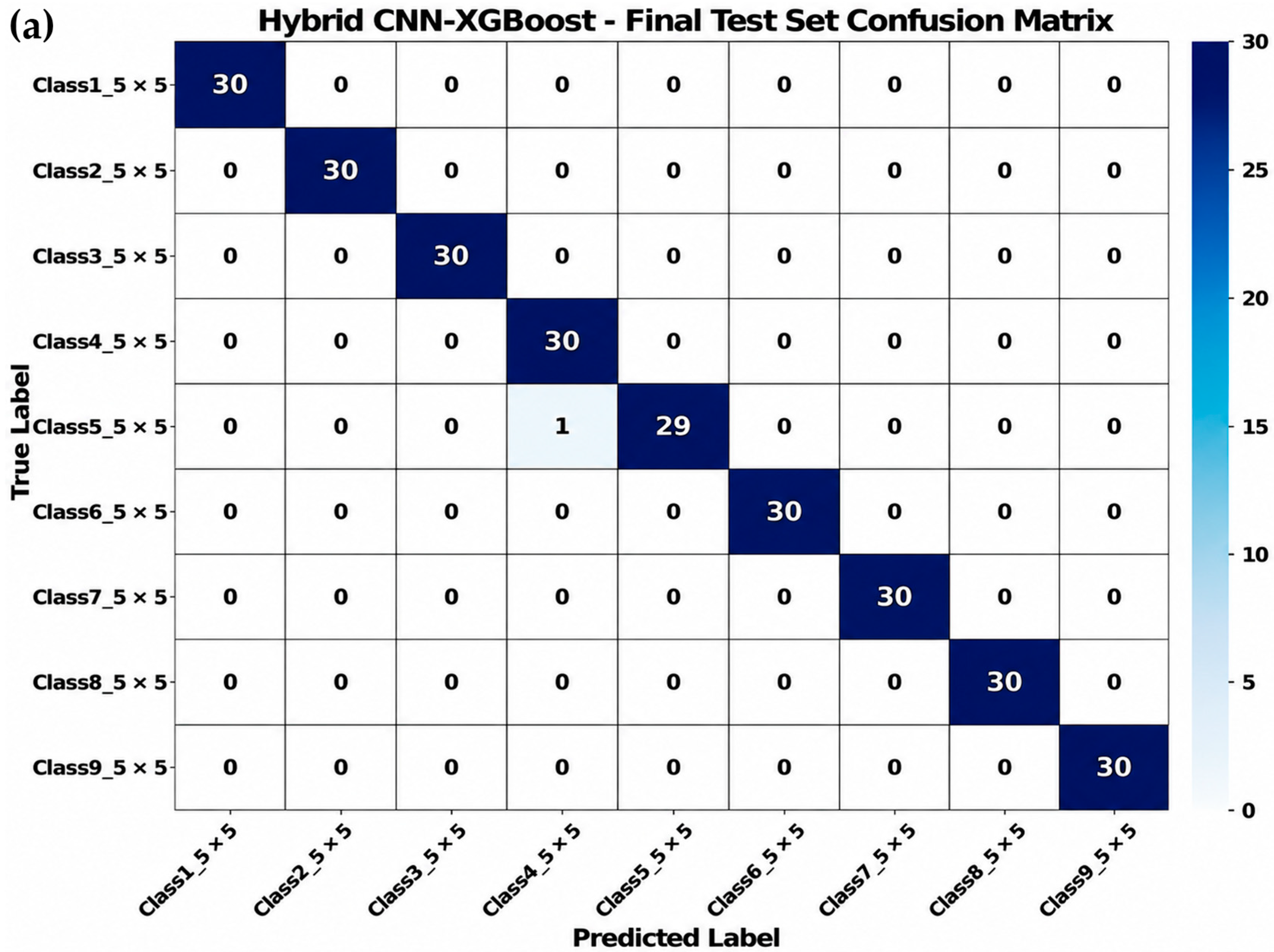
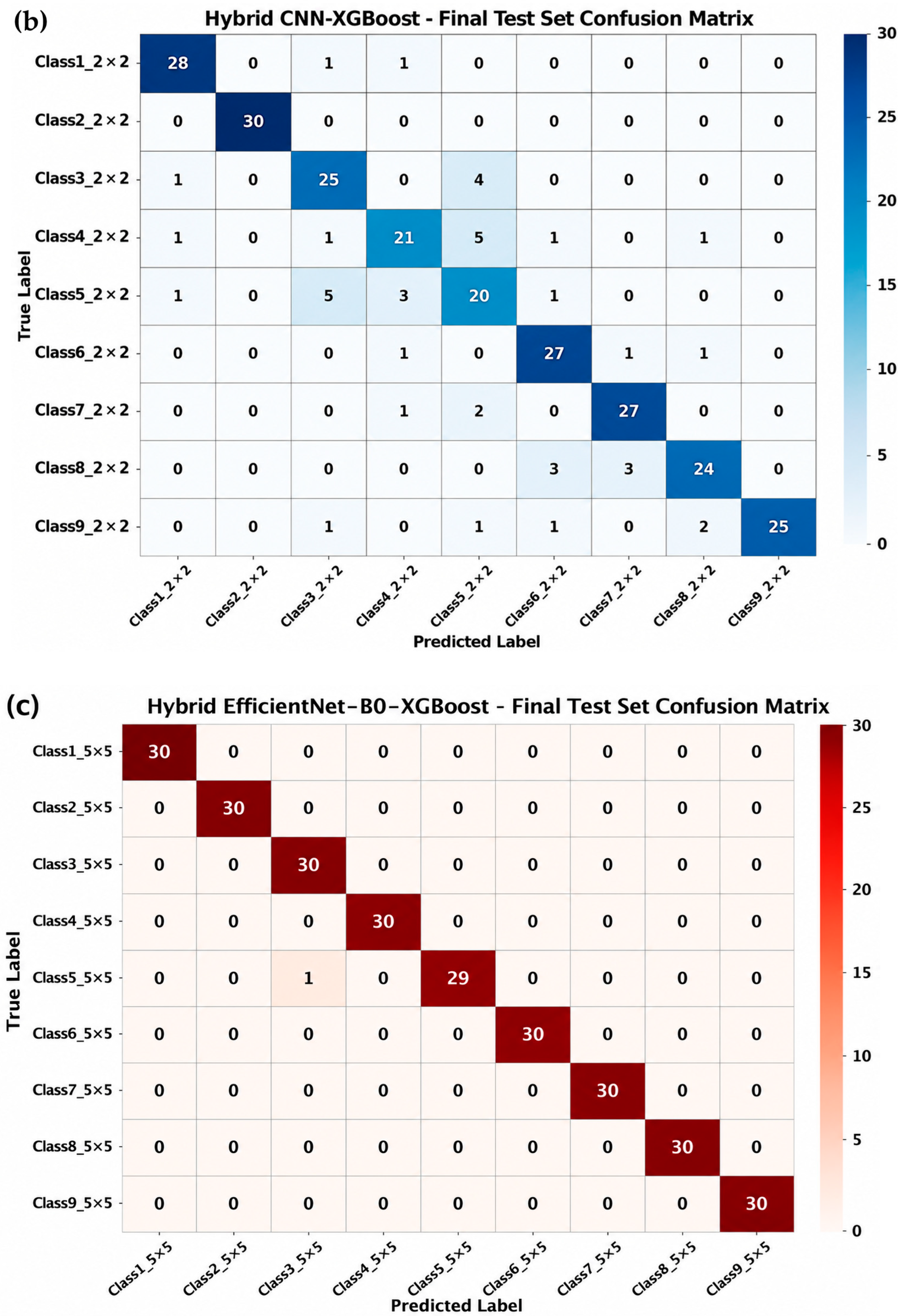
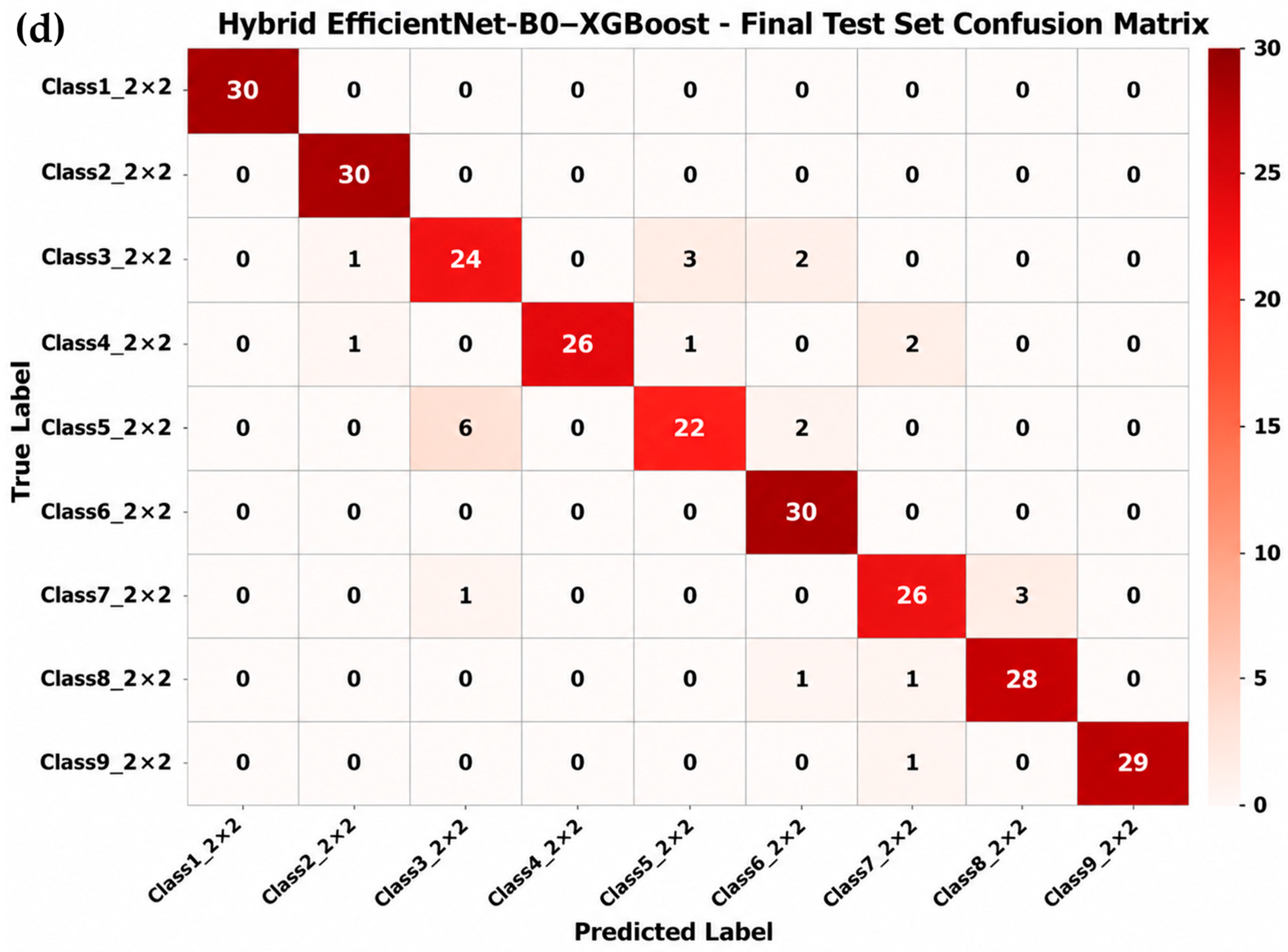
For the 2 × 2 m image analysis, the Hybrid EfficientNet-B0-XGBoost model clearly outperformed the Hybrid CNN-XGBoost model, achieving the highest classification accuracy of 0.900 ± 0.010 at 30 tuning units, whereas the highest accuracy of the Hybrid CNN-XGBoost model was 0.850 ± 0.022 at 50 tuning units. These findings indicate that the backbone architecture plays a critical role in classification performance when the available spatial context within the image is limited. The 2 × 2 m image patches were extracted from regions with high fish aggregation density, resulting in reduced cage-level contextual information, including fish distribution patterns, inter-fish spatial relationships, and surrounding spatial characteristics, compared with the 5 × 5 m images. Consequently, the models relied more heavily on the capability of the backbone architecture to extract fine-grained features from spatially constrained image data. These findings are consistent with previous studies related to spatial scale and contextual representation, which reported that image size and the amount of spatial context within an image directly influence the performance of DL models in learning object characteristics and spatial relationships within images [22,23,24,25].

The superior performance of the Hybrid EfficientNet-B0-XGBoost model for the 2 × 2 m images can be explained by the architectural characteristics of EfficientNet-B0, which was developed based on the compound scaling concept that systematically balances network depth, width, and image resolution. In addition, EfficientNet-B0 incorporates MBConv blocks, which improve deep feature extraction efficiency while maintaining an appropriate number of model parameters [20]. In the present study, EfficientNet-B0 was further optimized using a two-phase fine-tuning strategy. During phase 1, the backbone layers were frozen to preserve the general image features learned from the ImageNet dataset, whereas phase 2 involved fine-tuning all layers to enable the model to learn red tilapia-specific image characteristics, including body texture, scale patterns, color intensity, and surface shadow characteristics more effectively. This training strategy improved the capability of the model to extract fine-grained features associated with fish weight-range classification, particularly when the available spatial context within the image was limited. Furthermore, the MBConv structure and SE mechanism of EfficientNet-B0 enabled the model to selectively emphasize the most informative image features relevant to classification. These findings are consistent with previous studies demonstrating that EfficientNet-based architectures possess strong capabilities for analyzing complex image data across medical imaging, agricultural applications, and aquatic animal image classification tasks [10,11,12].

The findings of the present study are also consistent with those of Córdova et al. [19], who reported that EfficientNet-based architectures improved fish classification and weight estimation performance under highly complex and variable image conditions. Similar findings were reported by Feng et al. [16] and Zhou et al. [17], who demonstrated the effectiveness of EfficientNet-B0 for fish image analysis and complex underwater image classification tasks. In the present study, the Hybrid EfficientNet-B0-XGBoost model also achieved higher precision, recall, and F1-score values than the Hybrid CNN-XGBoost model for the 2 × 2 m images. These results indicate that EfficientNet-B0 not only improved overall classification accuracy but also enhanced the balance and consistency of classification performance across multiple evaluation metrics.

However, when using the 5 × 5 m images, the results showed that the Hybrid CNN-XGBoost model outperformed the Hybrid EfficientNet-B0-XGBoost model. The Hybrid CNN-XGBoost model achieved the highest classification accuracy of 0.988 ± 0.008 at 20 tuning units, whereas the highest accuracy of the Hybrid EfficientNet-B0-XGBoost model was 0.977 ± 0.021 at 40 tuning units. In addition, Hybrid CNN-XGBoost required a substantially shorter computational workflow time, with an average computational workflow time of only 0.038 ± 0.001 s per image, compared with 65.007 ± 6.141 s per image for Hybrid EfficientNet-B0-XGBoost. These findings suggest that when sufficient spatial context is preserved within the image, such as in the 5 × 5 m images that captured fish distribution patterns, stocking density, and aggregation behavior, conventional CNN architectures may already be capable of extracting the spatial features necessary for fish weight-range classification. Consequently, the advantages of EfficientNet-B0 become less pronounced relative to the substantially increased computational cost. This trend is consistent with previous studies reporting that patch size, spatial resolution, and spatial scale strongly influence DL model performance. Images that preserve sufficient contextual relationships between objects and their surrounding environments can improve the ability of DL models to learn spatial relationships more effectively [23,24,25]. Therefore, the present study demonstrates that the effectiveness of the backbone architecture is directly associated with image size and the amount of spatial context preserved within the image. EfficientNet-B0 appears to be more suitable for smaller image patches that require fine-grained feature extraction under limited spatial context conditions, whereas conventional CNN architectures may be more appropriate when images sufficiently capture the broader spatial context of the aquaculture system, such as the 5 × 5 m images used in this study, particularly in terms of both classification accuracy and computational efficiency. These findings further suggest that backbone selection for UAV-based fish weight-range classification should not rely solely on architectural complexity, but should also consider image size, spatial context availability, data resolution, and processing-time limitations under practical aquaculture conditions [22,26].

4.4. Practical Implications for Red Tilapia Aquaculture

The findings of the present study provide practical implications for red tilapia aquaculture, particularly in the development of non-invasive fish monitoring systems. The results demonstrated that UAV-based aerial imagery combined with hybrid DL models can accurately classify fish weight ranges without the need for frequent manual sampling and weighing. Such an approach may reduce labor requirements, minimize fish handling stress, and improve production management efficiency under commercial farming conditions. In addition, the findings suggest that image size and backbone selection should be considered according to operational objectives. Larger image patches preserving broader spatial context may be advantageous for routine farm-scale monitoring, whereas EfficientNet-B0-based models may provide additional benefits when image information is spatially constrained. Beyond red tilapia culture, the proposed framework may also be adapted for other cage-cultured fish species and precision aquaculture applications involving UAV-based monitoring, biomass assessment, and AI-assisted farm management.

4.5. Limitations and Future Work

Although the present study successfully developed hybrid DL models for red tilapia weight-range classification using UAV-based aerial imagery, several limitations should be considered in future investigations. Image acquisition in this study was conducted under relatively favorable environmental conditions, particularly during periods with suitable water quality and water transparency that allowed fish aggregation patterns to be clearly observed. Therefore, the performance of the models under low-transparency conditions, such as during the rainy season when water turbidity, suspended particles, and water surface reflections substantially increase, remains unclear. These environmental conditions may reduce the effectiveness of spatial feature extraction and limit the ability of the models to accurately detect fish aggregation patterns and morphological characteristics. Future studies should therefore incorporate image datasets collected under more diverse environmental conditions to improve model generalization capability and robustness in practical aquaculture environments.

In addition, most images used in this study were acquired before feeding, when fish tended to aggregate near the water surface, allowing clearer visualization of fish schools. However, the models were not evaluated under active feeding conditions, where rapid fish movement, water surface disturbances, and the presence of feed pellets substantially increase image complexity. Future research should therefore investigate the feasibility of image analysis during feeding periods to develop integrated AI systems capable of simultaneously evaluating fish weight ranges and feeding behavior from the same image dataset.

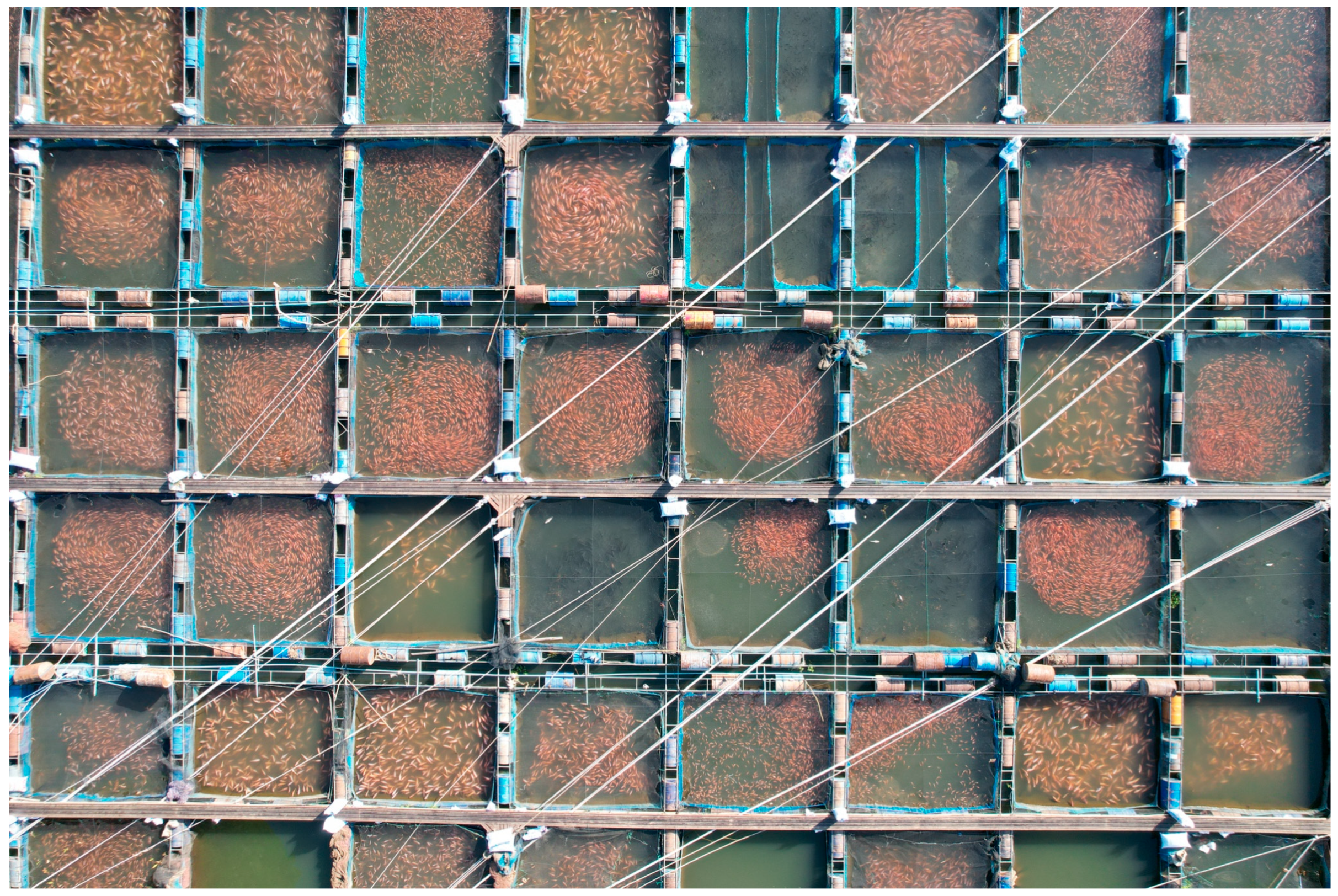
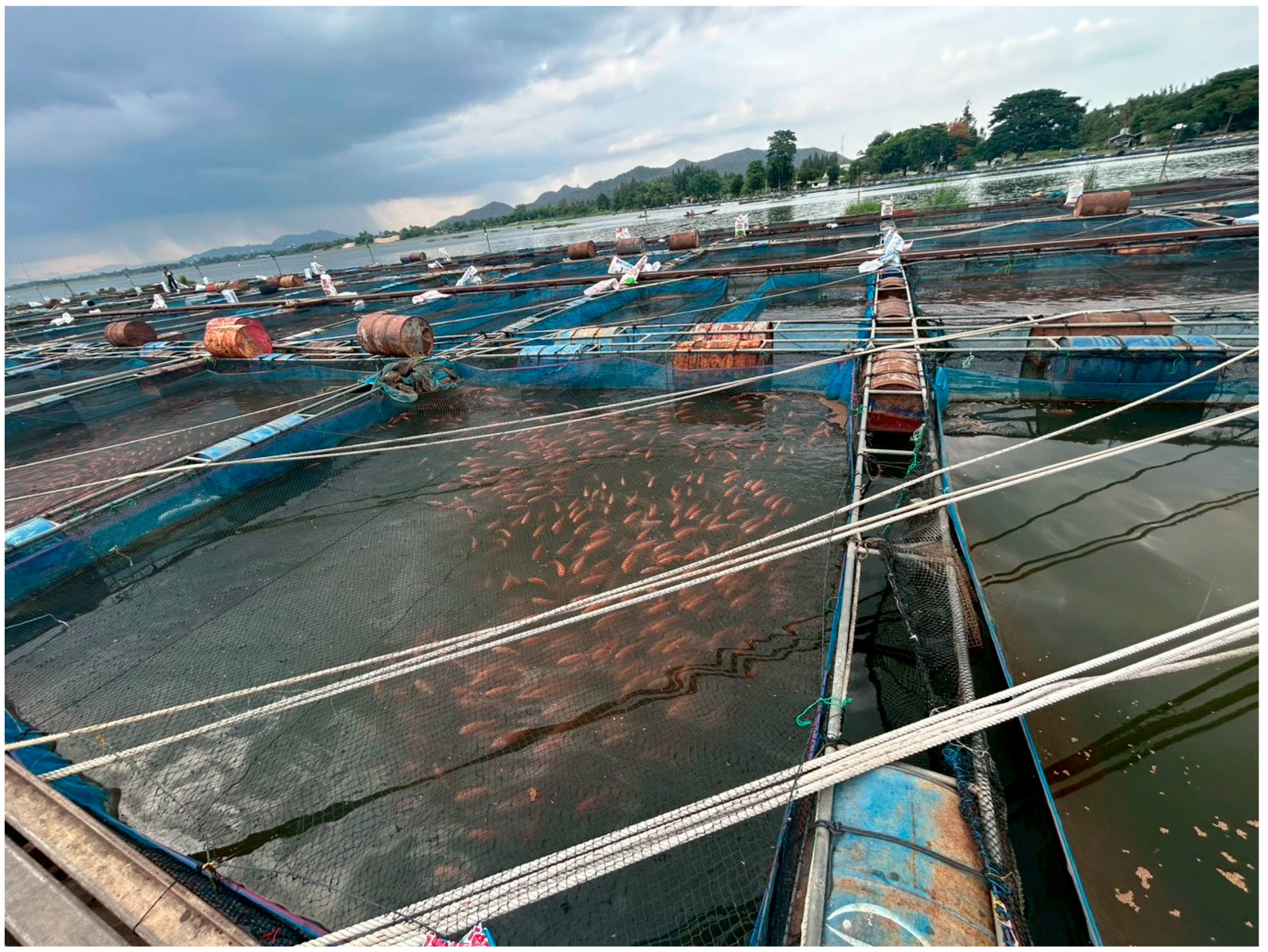
Another practical limitation associated with the use of large image patches, particularly the 5 × 5 m image size, is the presence of non-target objects commonly observed in commercial river cage aquaculture systems. As illustrated in Figure 10 and Figure 11, mooring ropes used to secure cages to the riverbank, cage structures, floating devices, feed bags, and other farming equipment are frequently present around cage boundaries and may be captured within UAV imagery. These objects can introduce background clutter, visual interference, and partial occlusion of fish aggregation areas, thereby reducing the effectiveness of feature extraction and potentially affecting model robustness under practical farming conditions. Although the fish-centered image extraction approach adopted in this study minimized some of these effects, the influence of non-target objects may become more pronounced in large-scale commercial farms where infrastructure density is considerably higher.

A further limitation of the present study is that the comparison was restricted to two hybrid frameworks, namely Hybrid CNN-XGBoost and Hybrid EfficientNet-B0-XGBoost. The primary objective of this study was to investigate the effects of image scale and backbone enhancement from CNN to EfficientNet-B0 within a hybrid learning framework. Therefore, standalone DL models, standalone XGBoost, traditional handcrafted image features, and comprehensive ablation experiments were not included in the present analysis. Although previous studies have demonstrated the effectiveness of hybrid learning approaches for fish weight classification, the relative contributions of individual model components could not be fully quantified within the scope of the current experimental design. Future studies should therefore perform comprehensive baseline comparisons and ablation analyses to further quantify the relative contributions of backbone architectures, classification algorithms, and image-scale effects on model performance.

Finally, the system developed in this study was based on offline image processing after UAV flight completion. Future developments should focus on real-world deployment through platforms or mobile applications capable of integrating UAV systems, AI-based image analysis, and mobile devices to enable near-real-time or real-time fish weight estimation and feeding behavior analysis immediately after image acquisition. Such advancement could further improve precision aquaculture management by reducing labor requirements, minimizing fish handling stress, and enhancing farm management efficiency under commercial aquaculture conditions.

5. Conclusions

This study proposed an artificial intelligence framework for red tilapia weight-range classification using UAV-based aerial imagery by comparing Hybrid CNN-XGBoost and Hybrid EfficientNet-B0-XGBoost models with two image sizes, namely 5 × 5 m and 2 × 2 m. The results demonstrated that both image size and backbone architecture directly influenced model performance. Overall, 5 × 5 m images consistently provided higher classification performance because they preserved broader spatial contextual information, including fish density, distribution patterns, and aggregation behavior. Under this condition, Hybrid CNN-XGBoost achieved the best overall performance, with the highest mean accuracy of 98.8% and a substantially shorter computational workflow time than Hybrid EfficientNet-B0-XGBoost, indicating that conventional CNN architectures remain highly effective when sufficient spatial context is available. In contrast, under the 2 × 2 m image condition, where spatial context was more limited, Hybrid EfficientNet-B0-XGBoost outperformed Hybrid CNN-XGBoost and achieved the highest mean accuracy of 90.0%, reflecting the superior capability of EfficientNet-B0 for fine-grained feature extraction through MBConv blocks, compound scaling, and attention-based feature extraction mechanisms. These findings indicate that larger images improve the ability of DL models to preserve both local object features and broader spatial relationships, whereas backbone enhancement from CNN to EfficientNet-B0 becomes more beneficial when image information is spatially constrained or highly complex. In addition, this study highlights the strong potential of integrating UAV technology with hybrid DL approaches for non-invasive fish weight monitoring in precision aquaculture systems, which can reduce labor requirements, minimize fish handling stress, and improve farm management efficiency. Therefore, Hybrid CNN-XGBoost with 5 × 5 m images demonstrated the best overall performance among the evaluated models under the experimental conditions of the present study, whereas Hybrid EfficientNet-B0-XGBoost with 2 × 2 m images represented a promising alternative when spatial context was limited.