Electronic Pulses as an Anti-Clogging Strategy for Drip Fertigation with Saltworks Bittern in Semi-Arid Regions

Abstract

Diluted solar saltworks effluent, applied via fertigation, can contribute to circular economy strategies by recycling nutrients and reducing the environmental impact associated with the disposal of hypersaline effluents. However, its adoption in drip irrigation systems is still limited, as are its effects on emitter performance. This study investigated whether electronic pulses could mitigate emitter clogging by applying dilution of saltworks bittern. Three systems (freshwater + saltworks bittern + electronic pulses; freshwater without electronic pulses; and freshwater + saltworks bittern without electronic pulses) were evaluated in Mossoró, Brazil, using three emitter designs over 0–320 h. Water physicochemical properties and hydraulic performance were monitored, and deposits were characterized by SEM—EDS and FTIR. Electronic pulses did not change bulk water chemistry but were associated with lower total suspended solids. Clogging risk was mainly related to alkaline pH, high electrical conductivity, and elevated Ca²⁺ and Mg²⁺ concentrations, which kept effluent dilutions within a high-risk range. Untreated effluent reduced irrigation uniformity, whereas treated effluent performed similarly to supply water. Electronic pulses reduced deposit complexity and the severity of critical events but did not eliminate clogging, and responses dependent on the emitter labyrinth’s geometry.

1. Introduction

Since antiquity, sodium chloride (NaCl) has played an important economic, cultural, and industrial role, remaining strategically relevant for food preservation, chemical manufacturing, pharmaceuticals, water treatment, and energy production [1,2,3,4,5,6]. Solar saltworks, widely established in coastal and semi-arid regions of countries such as China, the United States, India, Australia, Mexico, and Brazil, are socio-environmental systems shaped by climate, hydrology, soils, and human management [7,8]. In these systems, seawater is evaporated in shallow ponds, leading to sequential salt precipitation and NaCl harvesting. At the final crystallization stage, a highly concentrated residual brine, known as bittern, remains, containing Na⁺, Cl⁻, Mg²⁺, Ca²⁺, K⁺, SO₄²⁻, and trace elements such as Al, Br, Li, Sr, B, Cs, and Co [9,10]. Although traditionally treated as waste, bittern discharge may cause soil salinization, water contamination, biodiversity loss, and ecological imbalance when poorly managed [11,12,13,14]. However, its high concentration of macro- and micronutrients also creates opportunities for reuse and valorization as an alternative source of agricultural inputs, especially in regions where conventional fertilizers are costly or limited [15].

Global population growth has intensified food demand, requiring higher agricultural productivity on a limited land base and increasing dependence on mineral fertilizers and irrigation water, especially under climate variability [16,17]. This dependence is vulnerable because nitrogen fertilizers rely heavily on natural gas, while phosphorus and potassium fertilizers depend on mining activities concentrated in few countries, creating risks related to price volatility, supply disruptions, food security, and geopolitical tensions [18,19,20,21,22]. In this context, saline effluents from salt production, such as bittern, emerge as alternative nutrient sources. Beyond direct agricultural use, bittern can be valorized through selective ion recovery using chemical precipitation, ion exchange, membrane separation, electrodialysis, and solar-assisted crystallization to obtain Mg²⁺, K⁺, sulfate, and chloride salts for industrial or agricultural applications [23,24,25]. However, its use in agriculture requires careful management because crop responses depend on tolerance to salinity and specific ions [26]. When diluted or treated, bittern may supply nutrients and reduce fertilizer dependency, particularly in semi-arid systems, but excessive salinity can impair soil properties, plant water uptake, and crop productivity [27,28,29]. Therefore, safe application depends on balancing nutrient benefits with salinity-related risks.

In semi-arid regions, drip irrigation is essential for agricultural production because it improves water use efficiency, enables precise nutrient delivery, reduces evaporation, run-off, and deep percolation losses, and stabilizes crop water status under water-scarce conditions [30,31,32,33,34]. However, the use of saline waters or effluents, such as bittern, increases the risk of emitter clogging. This clogging may result from chemical precipitation of calcium carbonate, magnesium compounds, and sulfate salts; biological growth stimulated by nutrients or organic matter; and physical accumulation of suspended solids and crystallized salts [35,36,37]. Biofouling and bio incrustation further intensify this problem, as microbial biofilms can develop inside pipelines and emitter labyrinths, trapping particles and serving as nucleation sites for mineral precipitation [38,39,40]. Under saline and alkaline conditions, extracellular polymeric substances increase deposit cohesion, favoring mixed obstructions composed of biofilm, minerals, and fine particles. To mitigate these risks, conventional practices such as filtration, flushing, acidification, and chlorination remain widely used [41], while emerging approaches include magnetization, molecular oscillation devices, pulsating pressure, ultrasound, electrochemical treatments, antimicrobial materials, and biological control strategies [42,43,44,45,46,47,48,49]. Therefore, combining pre-treatment, operational management, and targeted anti-clogging technologies is essential for maintaining irrigation uniformity and enabling the sustainable reuse of saline effluents.

However, many of the currently employed mitigation methods involve high operational costs, frequent maintenance, and dependence on inputs that may not be readily available [50]. Chemical treatments require continuous monitoring and safe handling, filtration systems demand regular cleaning and replacement, and advanced treatment technologies may increase energy consumption and capital investment [51,52]. Therefore, although the use of freshwater mixed with saltworks bittern is attractive from a sustainability perspective, the economic and operational barriers associated with emitter clogging control may limit its practical adoption in drip fertigation systems. In this context, low-maintenance physical treatments may play an important role in improving technical feasibility and expanding the safe use of saline effluents for irrigation. Among these alternatives, electronic pulses have been proposed as a non-chemical treatment strategy to mitigate clogging by influencing precipitation, crystallization, particle aggregation, and deposition processes within hydraulic systems. Unlike chemical conditioning methods, electronic pulse treatment does not require the continuous addition of reagents and does not directly alter the bulk salinity of the water. Instead, dynamic electronic pulses may modify the crystallization behavior of dissolved ions, particularly Ca²⁺ and Mg²⁺ by the release of small amounts of carbonic acid during treatment may contribute to the gradual weakening of scale deposits, while the formation of suspended, less adherent particles may facilitate their transport through the system rather than their accumulation inside emitter labyrinths [53]. The underlying premise is that exposure to electromagnetic fields or pulsed electrical signals may affect ion association, particle aggregation, crystal nucleation, growth kinetics, and polymorphism, potentially reducing the adhesion and cohesion of mineral deposits within the irrigation network. Although such treatments do not remove dissolved salts, they may alter how and where scaling develops, delaying obstruction or promoting the formation of deposits that are less adherent and more easily transported or filtered.

Despite its potential, the use of bittern in agriculture as fertigation, remains underexplored and faces technical, regulatory, and social barriers. The variability in composition, high salinity levels, and lack of standardized application guidelines require further research and field validation [54]. Beyond agriculture, the reuse of bittern and other saline by-products has implications for broader sustainability goals. The valorization of materials in their natural or minimally processed form reduces the need for energy-intensive industrial transformations, contributing to lower carbon footprints [55,56]. Compared to conventional fertilizers derived from fossil fuels or petroleum-based processes, saline effluents represent a low-energy alternative with potential climate benefits. Reducing dependence on petroleum-derived inputs aligns with global efforts to decarbonize production systems and transition toward renewable and nature-based solutions [57,58]. Salt production through solar evaporation is inherently low in energy consumption compared to other mineral extraction processes, when by-products such as bittern are reused rather than discarded, the overall carbon footprint of the system can be further reduced.

This integrated approach enhances resource efficiency and supports the development of sustainable supply chains, particularly in regions vulnerable to climate variability and economic constraints. The reuse of saline effluents also contributes directly to several United Nations Sustainable Development Goals (SDGs). These include SDG 2 (Zero Hunger) through improved nutrient availability and agricultural productivity; SDG 6 (Clean Water and Sanitation) by promoting responsible water management and reuse; SDG 12 (Responsible Consumption and Production) through waste valorization and circular practices; and SDG 13 (Climate Action) by reducing greenhouse gas emissions associated with conventional fertilizer production. In this sense, the integration of salt production and agriculture represents a practical pathway toward achieving global sustainability targets.

Although saltworks bittern has been recognized as a saline by-product with potential for nutrient reuse and circular-economy applications, its use in drip fertigation remains poorly explored, particularly under semi-arid conditions. There is limited evidence on whether non-chemical physical treatments, such as electronic pulses, can mitigate emitter clogging by modifying precipitation, particle aggregation, and deposit adhesion without reducing bulk salinity. Moreover, few studies have linked water-quality dynamics, emitter hydraulic performance, and the morphology and elemental composition of clogging deposits.

This study assessed the feasibility of using freshwater mixed with saltworks bittern in drip fertigation and examined whether electronic pulse treatment could reduce emitter clogging under semi-arid conditions. We hypothesized that, although this physical treatment does not decrease total water salinity, it can influence precipitation dynamics, particle aggregation, and adhesion processes, thereby reducing the formation of cohesive deposits and improving hydraulic performance compared with untreated freshwater mixed with saltworks bittern.

To address this hypothesis, the physicochemical variability of three water sources was monitored throughout the experimental period: freshwater mixed with saltworks bittern and treated with electronic pulses, freshwater without electronic pulses, and freshwater mixed with saltworks bittern without electronic pulses. Concurrently, the hydraulic performance and water application uniformity of three drip tapes equipped with non-pressure-compensating emitters were evaluated during system operation. The morphology and elemental composition of the deposits formed inside the emitters were subsequently characterized by scanning electron microscopy coupled with energy-dispersive X-ray spectroscopy, enabling the hydraulic responses to be linked to water quality, treatment conditions, and clogging mechanisms.

2. Materials and Methods

2.1. Experimental Conditions and Source Water

The experiment was conducted between April and May 2025 in the outdoor area of the Laboratory of Rural Constructions and Environmental Comfort at the Federal Rural University of the Semi-Arid Region (UFERSA), located in Mossoró, Rio Grande do Norte, Brazil (5°12′13.14″ S; 37°19′26.93″ W), at approximately 16 m above sea level. The experimental area is part of the Brazilian Semi-arid Region and has a BSh climate (hot semi-arid), according to the Köppen classification, with a mean annual air temperature of 26.5 °C and average annual precipitation of 794 mm [59].

Three water sources were used in the experimental trials: (i) a saline effluent from a solar saltwork; (ii) freshwater provided by the Water and Sewage Company of Rio Grande do Norte (CAERN), applied in only one bench as the control; and (iii) desalinated water supplied by UFERSA’s Laboratory of Soil, Water, and Plant Analysis (LASAP), used to maintain reservoir volume and stabilize salinity levels in the three bench reservoirs throughout the experimental period.

2.2. Experimental Design

The experiment was arranged as a split-plot design under a completely randomized design, with three replications per water source, corresponding to the three drip-tape lines installed within each bench. Since each water source was represented by a single bench, the main water source effect was interpreted cautiously. The drip lines within each bench were treated as subsamples for the water source factor, and not as independent bench replicates. Thus, the statistical interpretation prioritized the decomposition of interactions and hydraulic patterns observed over time for each combination of water source, dripper type, and operating time. The main plots consisted of three water sources (bench treatments): WS1 = freshwater mixed with saltworks bittern and treated with electronic pulses; WS2 = freshwater without electronic pulses; and WS3 = freshwater mixed with saltworks bittern without electronic pulses. The subplots corresponded to the three drip-tape designs (D1, D2, and D3), which were installed in each bench in a randomized arrangement, with three lines per design (nine drip lines per bench). The sub-subplots were the repeated measurements over nine operating times (0, 40, 80, 120, 160, 200, 240, 280, and 320 h), used to monitor hydraulic performance and clogging progression throughout the experimental period.

2.3. Experimental Setup and Operation of the Drip Units

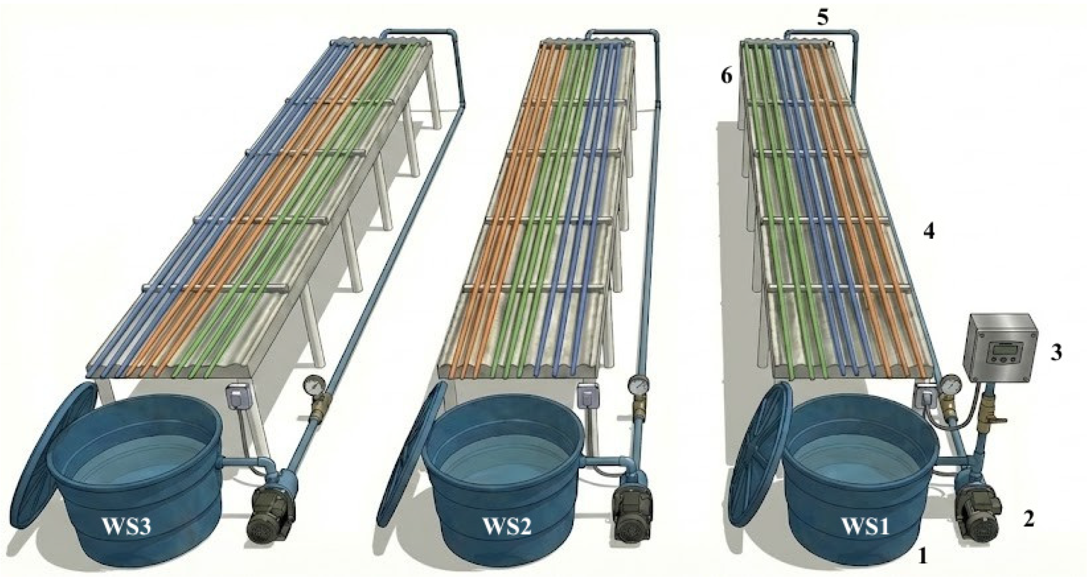
Three test benches, corresponding to water sources WS1, WS2, and WS3, were set up to conduct the experiment. Each bench had dimensions of 1.0 m × 8.3 m, totaling 8.30 m² of experimental area. The units were built on reinforced concrete supports and equipped with wooden structures designed to support corrugated fiber cement tiles, installed with a slope of 2.5%. This gradient allowed the applied water to flow by gravity, enabling its collection and subsequent recirculation in the system [60].

Each bench consisted of a water reservoir with a capacity of 0.31 m³ and a drip irrigation system as described in [53] consisting of: a 368 W pump-motor unit, a 120 mesh disc filter, a ball valve, a sampling point positioned after the filtration stage, and two pressure gauges for monitoring the system pressure. One of the pressure gauges was permanently installed before the filter, while the other, portable one, was used at the ends of the lateral lines. The system also included a 32 mm PVC main pipe, a 50 mm PVC branch line, nine ring-sealed connectors, and nine 16 mm diameter high-strength polyethylene lateral lines equipped with self-cleaning valves at the ends, as shown in Figure 1. Only bench WS1 received the installation of the electronic pulse generator.

WS1 operated during the full 6 h daily operating period using an ecological water-treatment device (0.15 m × 0.18 m), designed for pipes up to 1½”, with a maximum flow capacity of 3.0 m³ h⁻¹, power consumption of 4.3 W, and operating frequency between 3 and 32 kHz [61]. The system works through physical water treatment, in which electronic pulses interfere with calcium crystallization, making calcium carbonate crystals less prone to attach to internal surfaces and, therefore, limiting scale buildup.

The lateral lines were arranged along the 8.30 m benches using thin-walled drip tape with flat, non-pressure-compensating emitters, a configuration commonly adopted in melon production areas of Rio Grande do Norte and Ceará. Each bench received nine lateral lines; all fitted with drip tape designed for short-cycle use (1–3 crops). The emitters had the following specifications:

D1 = self-cleaning design, nominal discharge of 1.6 L h⁻¹ at 100 kPa, flow coefficient of 0.693, flow exponent (x) of 0.45, filtration area of 24 mm², water passage dimensions of 0.66 × 0.63 × 18 mm (width × depth × length) with 0.4 m emitter spacing, and wall thickness of 0.25 mm and recommended filtration of 80 mesh.

D2 = self-cleaning design, nominal discharge of 1.6 L h⁻¹ at 100 kPa, flow coefficient of 0.568, flow exponent (x) of 0.45, filtration area of 15 mm², water passage dimensions of 0.65 × 0.55 × 13 mm (width × depth × length), with 0.4 m emitter spacing, wall thickness of 0.20 mm and recommended filtration of 120 mesh.

D3 = self-cleaning design, nominal discharge of 2.0 L h⁻¹ at 100 kPa, flow coefficient of 0.693, flow exponent (x) of 0.46, filtration area of 54 mm², water passage dimensions of 0.76 × 1.03 × 65 mm (width × depth × length) with 0.4 m emitter spacing, and wall thickness of 1.00 mm and recommended filtration of 80 mesh.

All benches operated for an average of 6 h per day until a cumulative operating time of 320 h was reached over consecutive days, to induce emitter clogging under controlled experimental conditions. Pressure at the end of the lateral lines was checked throughout the trial and kept at 80 kPa using a portable pressure gauge (0 to 400 kPa range). This pressure level was adopted because it is commonly used in drip irrigation systems and can favor clogging in narrow emitter passages when water quality is restrictive. The 0.31 m³ reservoirs were replenished every two days to offset evaporation losses, since the benches were exposed to outdoor conditions. At the end of each 40 h cycle, the water was completely replaced, and the reservoir was cleaned before refilling. Whenever water salinity exceeded the initial 0 h value by more than 10%, low salinity desalinated water (electrical conductivity of 0.020 to 0.040 dS m⁻¹) was added to recover the reservoir volume and keep salinity levels stable throughout the experiment.

The 320 h operating period was adopted to simulate an accumulated irrigation time equivalent to approximately two melon crop cycles under semi-arid conditions in Rio Grande do Norte, Brazil. This period represents a critical operating condition in which drip irrigation systems using waters with high clogging potential may show substantial hydraulic performance losses, often requiring lateral line replacement when CUC < 80% and AFRV < 75%.

2.4. Physicochemical Characterization of the Three Water Sources Throughout the Operation of the Experimental Units

To monitor the clogging risk of the three water sources used in the experimental benches, samples from WS1, WS2, and WS3 were collected downstream of the filtration system at nine operating intervals (0, 40, 80, 120, 160, 200, 240, 280, and 320 h), in accordance with Standard Methods for the Examination of Water and Wastewater—APHA [62]. Water temperature (WT) and electrical conductivity (EC) were determined in the field between 06:00 and 12:00 using a mercury thermometer and a portable conductivity meter, respectively.

All collected samples were sent to LASAP/UFERSA for laboratory analysis. The following parameters were determined: pH by direct measurement with a pH meter; Ca²⁺ and Mg²⁺ by EDTA complexometric titration (using Eriochrome Black T as the indicator for magnesium and calcon for calcium); Fe and Mn by inductively coupled plasma optical emission spectrometry (ICP—OES); and total suspended solids (TSS) by the gravimetric method at 103 to 105 °C, following procedures recommended by APHA [62] and the Brazilian Agricultural Research Corporation-Embrapa [63].

To classify the dripper clogging risk of the three water sources as low, moderate, or severe, the criteria proposed by [64] were used for TSS, EC, Ca²⁺, Mg²⁺, Fe and Mn, whereas the criteria of [65] were applied to pH.

2.5. Monitoring of Hydraulic Performance and Emitter Clogging

Sixteen emitters were selected on each lateral line of the experimental benches for flow-rate monitoring, following an adapted procedure on [66], to evaluate hydraulic and anti-clogging performance for the three water sources. Every 40 h of operation, flow rates were measured by collecting discharged water in 250 mL plastic containers with the counting time fixed at 5 min, where the collected liquid was measured using graduated beakers, in accordance with an adaptation of the NBR ISO 9261 recommendations [67].

Emitter clogging and hydraulic performance were quantified using two indicators: (i) AFRV = average flow-rate variation rate [64] (Equation (1)); and (ii) CUC = distribution uniformity coefficient [68] (Equations (2) and (3)).

$$\mathrm{A}\mathrm{F}\mathrm{R}\mathrm{V}={\displaystyle \frac{{\displaystyle {\sum }_{\mathrm{i}=1}^{\mathrm{n}}}\frac{{\mathrm{q}}_{\mathrm{a}}}{{\mathrm{q}}_{\mathrm{i}}}}{\mathrm{n}}}\times 100$$

(1)

where AFRV = average flow-rate variation rate, %; qₐ = current emitter flow rate, L h⁻¹; qᵢ = initial emitter flow rate, L h⁻¹; and n = number of emitters evaluated.

AFRV values were classified according to the criterion proposed by [69], as follows: AFRV ≥ 95%, no clogging; 80% ≤ AFRV < 95%, slight clogging; 50% ≤ AFRV < 80%, partial clogging; 25% ≤ AFRV < 50%, severe clogging; and AFRV ≤ 25%, complete clogging.

$${\mathrm{q}}_{\mathrm{m}}={\displaystyle \frac{{\displaystyle {\sum }_{\mathrm{i}=1}^{\mathrm{n}}}{\mathrm{q}}_{\mathrm{a}}}{\mathrm{n}}}$$

(2)

$$\mathrm{C}\mathrm{U}\mathrm{C}={\displaystyle \frac{{\displaystyle {\sum }_{\mathrm{i}=1}^{\mathrm{n}}}|{\mathrm{q}}_{\mathrm{a}}-{\mathrm{q}}_{\mathrm{m}}|}{\mathrm{n}\times {\mathrm{q}}_{\mathrm{m}}}}\times 100$$

(3)

where CUC = Christiansen’s Uniformity Coefficient, %; q_a = current emitter flow, L h⁻¹; q_m = mean emitter flow rate, L h⁻¹; and n = number of evaluated emitters.

CUC values were classified according to the criterion proposed by [70], as followed: CUC > 90% was classified as excellent; 80% ≤ CUC ≤ 90% as good; 70% ≤ CUC < 80% as fair; and CUC < 70% as poor.

2.6. Scanning Electron Microscopy (SEM) and Energy-Dispersive X-Ray Spectroscopy (EDS) Analyses

For micrographic analysis using scanning electron microscopy coupled with energy-dispersive X-ray spectroscopy (SEM—EDS), emitters that showed visible biodeposition in their labyrinths were selected. Samples were collected in duplicate from the final third of the lateral lines, the region with the highest concentration of obstructive material, in the benches supplied with the three water sources (W1, W2, and W3). In total, 54 samples were analyzed, corresponding to the three types of emitters removed from the lateral lines subjected to the three water sources.

After collection, the emitters were carefully removed from the lateral lines and placed in a desiccator for 72 h to reduce excess moisture before sample preparation. Subsequently, sections of approximately 10 mm from the labyrinthine channels containing obstructive material were cut and mounted on 12.5 mm diameter aluminum supports using adhesive tape.

Next, duplicate samples were mounted on metal stubs using conductive carbon tape (PELCO Tabs™, Ted Pella, Inc., Redding, CA, USA) and sputter coated (Q150R ES, Quorum Technologies Ltd., Laughton, East Sussex, UK) with a thin gold layer (9 nm). This coating enhanced sample conductivity and enabled the acquisition of high-quality images. SEM micrographs were then obtained using a secondary electron detector in a scanning electron microscope (VEGA 3 LMU, Tescan, Brno, Czech Republic) operated at an accelerating voltage of 20 kV, following the recommendations of [71]. Images were captured at magnifications of 30×, 40×, 100×, 1700×, and 5000×, with the highest magnification providing the greatest level of structural detail.

On the same set up sample, Energy-dispersive X-ray spectroscopy (EDS) analyses were performed using an Xplore System detector (Oxford Instruments NanoAnalysis, High Wycombe, UK) operated with AZtecOne software (Oxford Instruments NanoAnalysis, High Wycombe, UK). According to the manufacturer specifications, the detector provides a guaranteed 129 eV Mn Kα resolution at 5.9 keV [72,73].

Fourier-transform infrared spectroscopy-FTIR ((Agilent Technologies, Santa Clara, CA, USA)) was used to identify functional groups associated with organic and inorganic constituents in the deposits formed inside the emitters after 320 h of operation. For each water source treatment (WS1, WS2, and WS3), 30 emitters were collected from the final third of the lateral lines, including 10 emitters of each model: D1, D2, and D3. The emitters were carefully dissected, and the clogging material adhered to the internal labyrinth region was manually removed. The material obtained from the 30 individual emitters was homogenized to form one composite sample per water source, with an approximate mass of 5 mg, which was subsequently used for FTIR analysis.

The FTIR analyses of the composite deposit samples obtained from WS1, WS2, and WS3 were performed in partnership with the laboratory of the Núcleo de Pesquisa em Economia de Baixo Carbono (NPCO₂) at UFERSA. The spectra were obtained using an Agilent Cary 630 FTIR spectrophotometer equipped with a ZnSe crystal and an attenuated total reflectance (ATR) Diamond Module accessory. The analyses were performed in the wavenumber range of 4000–650 cm⁻¹, with a spectral resolution of 4 cm⁻¹. For each composite sample, the final spectrum was generated from the arithmetic mean of eight scans.

2.7. Statistical Analysis

Water quality data, referring to WT, TSS, EC, pH, Ca²⁺, Mg²⁺, Mn, and Fe (n = 27), were initially assessed for normality of residuals using the Shapiro–Wilk test, adopting p > 0.05 as the criterion for not rejecting the normality hypothesis. When the normality assumptions were met, analysis of variance (ANOVA; F-test; p ≤ 0.05) was applied, followed by multiple comparisons between water sources. When normality was not met, the Aligned Rank Transform (ART) procedure, suitable for non-parametric factor analysis, was used. In all cases, the p-values of the multiple comparisons were adjusted using the Benjamini–Hochberg method, controlling for the false discovery rate (FDR).

The ART procedure was applied following the split-split-plot model under a completely randomized design. For each response variable, the full factorial model is:

$${\mathrm{Y}}_{\mathrm{i}\mathrm{j}\mathrm{k}\mathrm{l}}=\mathsf{\mu }+{\mathrm{A}}_{\mathrm{i}}+{\mathrm{B}}_{\mathrm{j}}+{\mathrm{C}}_{\mathrm{k}}+(\mathrm{A}\mathrm{B}{)}_{\mathrm{i}\mathrm{j}}+(\mathrm{A}\mathrm{C}{)}_{\mathrm{i}\mathrm{k}}+(\mathrm{B}\mathrm{C}{)}_{\mathrm{j}\mathrm{k}}+(\mathrm{A}\mathrm{B}\mathrm{C}{)}_{\mathrm{i}\mathrm{j}\mathrm{k}}+{\mathsf{\epsilon }}_{\mathrm{i}\mathrm{j}\mathrm{k}\mathrm{l}}$$

(4)

where $Y_{ijkl}$ = the observed response, $\mu$ = overall mean, $A_i$ = effect of water source ($i=1,2,3$), $B_j$ = effect of dripper ($j=1,2,3$), $C_k$ = effect of operating time ($k=1,\dots ,9$), the parenthetical terms their interactions, and ${\epsilon }_{ijkl}$ = residual error.

For each effect of interest, the ART aligns the response by removing all model effects except the one being tested. The aligned response for a given effect $T$ is

$${\mathrm{Y}}_{\mathrm{i}\mathrm{j}\mathrm{k}\mathrm{l}}^{\prime }={\mathrm{Y}}_{\mathrm{i}\mathrm{j}\mathrm{k}\mathrm{l}}-{\widehat{\mathsf{\mu }}}_{\mathrm{full}}+{\widehat{\mathsf{\tau }}}_{\mathrm{T}}$$

(5)

where ${\widehat{\mu }}_{\mathrm{full}}$ = the fitted value from the full model excluding effect $T$, and ${\widehat{\tau }}_T$ = estimated cell effect attributable to $T$. The aligned values are then converted to ranks, and the ANOVA is performed on these ranks, so that each F-test isolates a single effect. For comparisons within significant interactions, the aligned rank transform for contrasts (ART-C) was used, which performs the alignment specifically for each contrast rather than for the main effect.

For the hydraulic performance and emitter clogging indicators, AFRV and CUC (n = 243), the normality of the residuals was assessed using the Shapiro–Wilk test, and the homogeneity of variances using Levene’s test. The experimental design considered was a split-split-plot design, with water source (A), dripper type (B), and operating time (C). Since each water source was conducted on a single bench, the drip lines within each bench were interpreted as subsamples for the water source factor, and not as independent replicates of that factor. Thus, the isolated main effect of water source was interpreted with caution.

When the parametric assumptions were met, the data were analyzed by ANOVA, respecting the error strata of the design. When the assumptions were not met, ART was used. For significant interactions, especially the water source × dripper type × operating time interaction, ART-C contrast decompositions were performed. This procedure was adopted instead of simple global rank transformation because it allows for the correct evaluation of effects and contrasts in factorial structures.

Effect sizes were estimated by eta-squared (η²), with 95% confidence intervals, and classified as negligible (η² < 0.01), small (0.01 ≤ η² < 0.06), medium (0.06 ≤ η² < 0.14), or large (η² ≥ 0.14). All statistical analyses, diagnostics, and figures were performed using R software version 4.6.0 [74].

3. Results

3.1. Water Quality Characterization Under Different Treatment Conditions

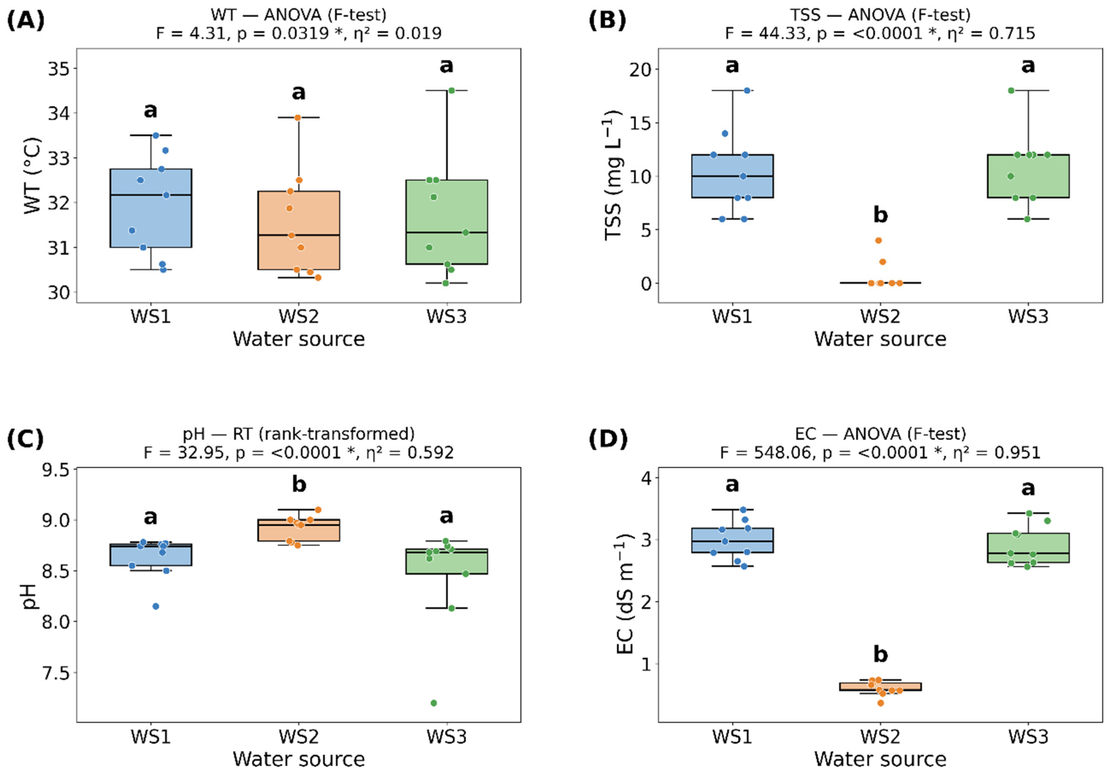
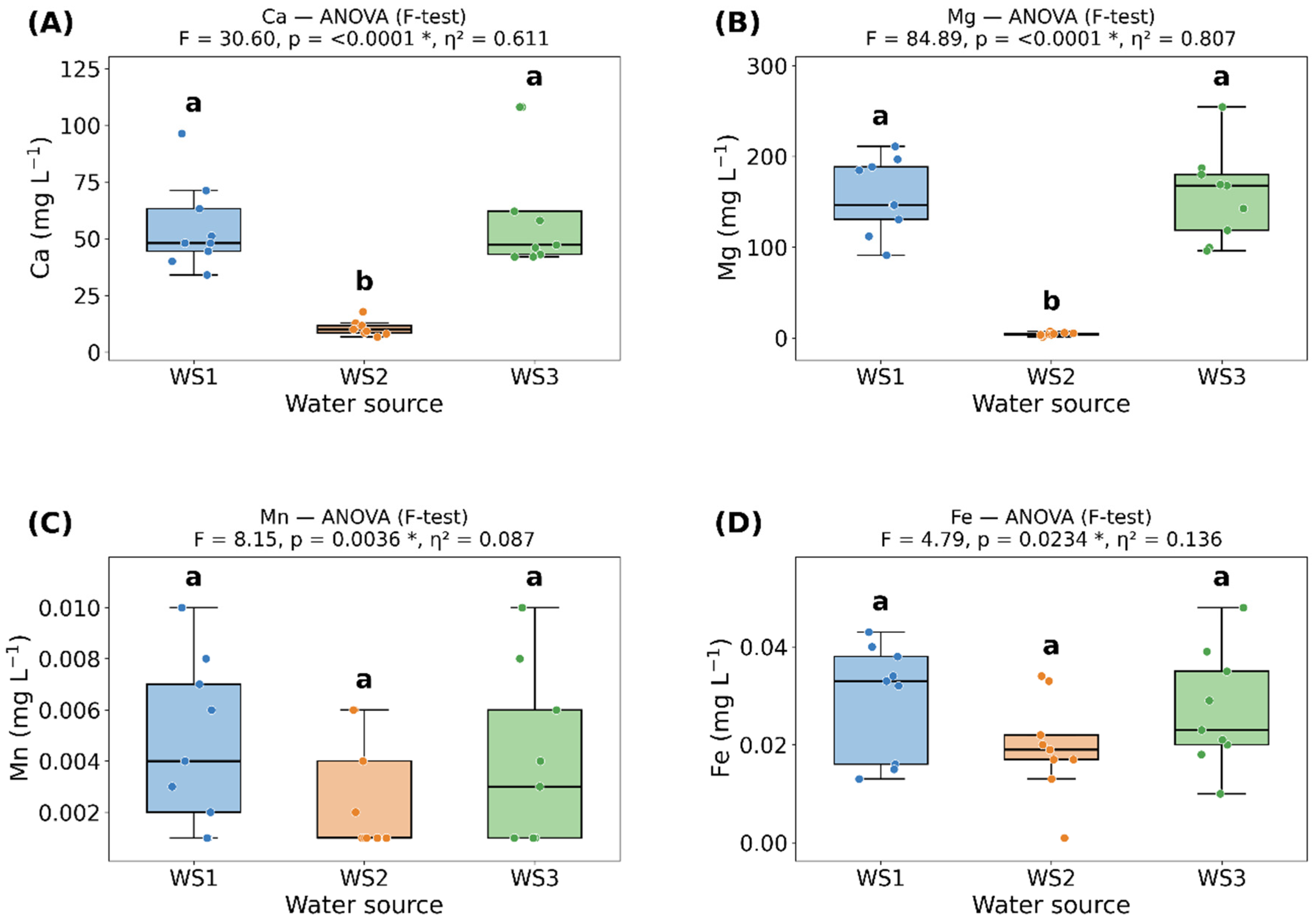
Figure 2 and Figure 3 show the distribution of physicochemical parameters for the evaluated water sources, based on measurements collected at nine sampling times during the experimental period (0, 40, 80, 120, 160, 200, 240, 280, and 320 h). Significant differences were observed for all eight evaluated parameters across treatment conditions, enabling differentiation among WS1, WS2, and WS3. Results are expressed as medians with interquartile ranges, and statistically significant differences are indicated by distinct letters (p < 0.05).

WT showed a small but statistically significant difference among treatments (p = 0.0319, η² = 0.019), although medians remained very close (32, 31, and 31 °C for WS1, WS2, and WS3, respectively) with strong overlap, indicating broadly similar thermal conditions. In contrast, TSS clearly differed among treatments (p < 0.0001, η² = 0.715): WS2 presented null values (0 mg L⁻¹), whereas both bittern waters showed higher concentrations, with a 16.7% lower median TSS in WS1 than in WS3. pH and EC also differed significantly among treatments (pH: p < 0.0001, η² = 0.592; EC: p < 0.0001, η² = 0.951), with WS2 exhibiting higher pH (median 8.95) and lower EC (median 0.58 dS m⁻¹) than WS1 and WS3, which remained at elevated and statistically similar with EC values of median 2.97 and 2.78 dS m⁻¹, respectively, and slightly lower pH, 8.74 and 8.68, respectively (Figure 2).

Ca²⁺ and Mg²⁺ differed strongly among treatments (p < 0.0001, η² = 0.611 for Ca²⁺ and p < 0.0001, η² = 0.807 for Mg²⁺). WS2 showed lower concentrations of median Ca²⁺ 10 mg L⁻¹ and median Mg²⁺ 3.96 mg L⁻¹, whereas WS1 and WS2 presented elevated and comparable values, with median Ca²⁺ 48 and 47.2 mg L⁻¹, respectively, and values of median Mg²⁺ 146.4 and 168 mg L⁻¹, respectively. Nevertheless, relative to WS3, WS2 showed a 12.9% reduction in median Mg²⁺ and a 14.3% decrease in the Mg²⁺/Ca²⁺ ratio. Mn and Fe also showed significant overall treatment effects (Mn: p = 0.0036, η² = 0.087; Fe: p = 0.0234, η² = 0.136), but the post hoc grouping indicates more subtle separation; still, median Fe and Mn in WS1 were higher than in WS3 by 43.5% and 33.3%, respectively (0.033 and 0.023 mg L⁻¹ for Fe; 0.004 and 0.003 mg L⁻¹ for Mn, respectively) (Figure 3).

3.2. ART Analysis (Aligned Rank Transform) with Bonferroni Post Hoc Test

Prior to the statistical analysis, the normality of the model residuals was assessed using the Shapiro–Wilk test. The results indicated a lack of normality for both AFRV (W = 0.93, p < 0.001) and CUC (W = 0.50, p < 0.001), showing that the data did not adequately meet the assumptions of a conventional parametric analysis.

Accordingly, the Aligned Rank Transform (ART) procedure was adopted, which is more appropriate for data with a factorial structure when residual normality is not met. For comparisons within significant interactions, the ART-C procedure was applied, with p-values adjusted by the Benjamini–Hochberg false discovery rate (FDR) method to control for the false discovery rate across multiple comparisons.

The analysis of variance was then conducted considering the split-split-plot structure under a completely randomized design. The ANOVA results for each response variable are presented in

Table 1. ANOVA on ranks (ART) for AFRV (%) and CUC (%) in a completely randomized design with a split-split-plot arrangement.

Source	Df	SQ Ranks	QM Ranks	F	p-valor	η2	Sig.
Water source (A)	2	9364.96	4682.48	2.1996	0.192068	0.0078	ns
Error (a)	6	12,772.74	2128.79			0.0107
Dripper (B)	2	25,001.19	12,500.59	1.6248	0.237430	0.0209	ns
A × B	4	103,569.93	25,892.48	3.3655	0.045721	0.0867	*
Error (b)	12	92,323.19	7693.60			0.0773
Time (C)	8	548,958.50	68,619.81	48.6258	0.000000	0.4597	***
A × C	16	34,270.04	2141.88	1.5178	0.100830	0.0287	ns
B × C	16	47,990.59	2999.41	2.1255	0.010082	0.0402	*
A × B × C	32	116,621.30	3644.42	2.5825	0.000071	0.0977	***
Error (c)	144	203,210.07	1411.18			0.1702
Total	242	1,194,082.50	0.00
Source	Df	SQ Ranks	QM Ranks	F	p-valor	η2	Sig.
Water source (A)	2	147,984.30	73,992.15	24.6243	0.001281	0.1238	**
Error (a)	6	18,029.09	3004.85			0.0151
Dripper (B)	2	246,577.90	123,288.95	26.3346	0.000041	0.2062	***
A × B	4	49,021.90	12,255.48	2.6178	0.088035	0.0410	ns
Error (b)	12	56,179.65	4681.64			0.0470
Time (C)	8	52,289.33	6536.17	2.1598	0.033934	0.0437	*
A × C	16	46,917.54	2932.35	0.9690	0.493625	0.0392	ns
B × C	16	45,063.38	2816.46	0.9307	0.535913	0.0377	ns
A × B × C	32	97,870.82	3058.46	1.0106	0.461380	0.0819	ns
Error (c)	144	435,782.59	3026.27			0.3645
Total	242	1,195,716.50	0.00

Note: A, B, and C—Represent the sources of variation isolated in the plots, subplots, and sub-subplots; a, b, and c—Represent the errors of the plots, subplots, and sub-subplots; Df = Degrees of Freedom; SQ = Sum of Squares; and QM = Mean Squar; *, **, *** Significant by F-test or rank transform (p ≤ 0.05; p ≤ 0.01; p ≤ 0.001); ns—Not significant by F-test or rank transform (p > 0.05).

.

For AFRV, the A × B × C triple interaction was significant (p = 0.000071), indicating that the effect of water sources on AFRV depends simultaneously on the emitter type and operating time. When the highest-order interaction is significant, the main effects and double interactions should not be interpreted in isolation. The non-significant A × B × C interaction for CUC (p = 0.4614) indicates that the combined effect of water source, emitter type, and operating time did not produce a response pattern beyond residual variability. Thus, the CUC responses were predominantly additive, with no evidence of dependence between the three factors. In factorial ANOVA, this is interpreted as the absence of a higher-order interaction, allowing emphasis on lower-order terms and main effects (when appropriate).

When the highest-order interaction (A × B × C) is significant, interpreting the individual effects and double interactions is inadequate, as the behavior of each factor depends on the combination of the other two. The decomposition consists of fixing two factors and comparing the levels of the third, using Error (c) as the error term and applying the ART-C procedure with FDR adjustment at a significance level of 5%.

Three types of decomposition are presented for AFRV: (i) Water Sources (A) within each Emitter × Time combination—assesses whether water sources differ for each emitter at each point in time (

Table 2. Comparison of water sources within each dripper × operating time combination for AFRV—significant combinations only (ART-C with FDR adjustment, α = 0.05).

Dripper	Time	WS1	Group	WS2	Group	WS3	Group	Ranking
D1	120 h	95.78	a	96.08	a	89.75	b	WS2a = WS1a > WS3b
D1	240 h	94.98	ab	95.03	a	97.84	b	WS3b > WS2a = WS1ab
D1	280 h	95.45	a	96.42	a	99.14	b	WS3b > WS2a = WS1a
D1	320 h	94.38	a	96.42	a	99.30	b	WS3b > WS2a = WS1a
D2	80 h	98.61	a	101.08	b	99.51	ab	WS2b = WS3ab = WS1a
D2	120 h	95.79	a	97.48	ab	99.51	b	WS3b = WS2ab = WS1a
D2	160 h	98.94	a	101.15	b	98.57	ab	WS2b > WS1a = WS3ab
D2	200 h	99.20	ab	101.14	a	98.67	b	WS2a = WS1ab = WS3b
D2	240 h	98.13	a	98.64	a	94.66	b	WS2a = WS1a > WS3b
D3	40 h	98.73	a	98.57	a	96.00	b	WS1a = WS2a > WS3b
D3	240 h	98.36	a	98.09	a	94.81	b	WS1a = WS2a > WS3b
D3	280 h	98.83	ab	99.64	a	96.66	b	WS2a = WS1ab = WS3b

); (ii) Emitters (B) within each Source × Time combination—assesses whether emitters differ for each source at each point in time (

Table 3. Comparison of drippers within each water source × operating time combination for AFRV—significant combinations only (ART-C with FDR adjustment, α = 0.05).

Source	Time	D1	Group	D2	Group	D3	Group	Ranking
WS1	80 h	100.77	ab	98.61	a	101.39	b	D3b = D1ab = D2a
WS1	120 h	95.78	ab	95.79	a	98.34	b	D3b > D2a = D1ab
WS1	280 h	95.45	a	97.09	ab	98.83	b	D3b = D2ab = D1a
WS2	240 h	95.03	b	98.64	a	98.09	a	D2a = D3a > D1b
WS2	280 h	96.42	a	98.92	ab	99.64	b	D3b = D2ab = D1a
WS3	120 h	89.75	b	99.51	a	99.46	a	D2a = D3a > D1b
WS3	240 h	97.84	b	94.66	a	94.81	a	D1b > D3a = D2a
WS3	280 h	99.14	a	97.14	ab	96.66	b	D1a = D2ab = D3b
WS3	320 h	99.30	a	97.09	ab	96.22	b	D1a = D2ab = D3b

); (iii) Time (C) within each Source × Emitter combination—assesses the temporal evolution for each source-emitter combination.

Of the 27 emitter × time combinations analyzed, 12 (44.4%) showed significant differences between water sources, while 15 combinations (55.6%) showed no differences. Detailed analysis by source revealed that the differences between WS1, WS2, and WS3 depended on both the type of dripper and the evaluation time. For dripper D1, WS3 tended to perform better in the later operating times (240 h, 280 h, and 320 h), suggesting that the WS3–D1 combination was more resistant to progressive clogging, although at 120 h this source showed the lowest value. For dripper D2, WS2 stood out during the intermediate to advanced period (80 h, 160 h, 200 h, and 240 h), indicating that this source provided better flow maintenance for this emitter. For dripper D3, WS3 showed the lowest values at 40 h and again at 240–280 h. These dynamic patterns reflect the complex interaction between water quality, the design characteristics of each dripper, and the kinetics of the clogging process.

Of the 27 water source × time combinations analyzed, 9 (33.3%) showed significant differences between emitters. The differences between emitters were observed in specific water source × time combinations. In WS1, D3 tended to be superior to D2 at intermediate to advanced times (80 h, 120 h, and 280 h). In WS2, emitters D2 and D3 outperformed D1 at 240 h, indicating that D1 was more susceptible to clogging when operating with this source, while at 280 h D3 stood out. In WS3, D1 was superior at 280 h and 320 h, while D2 and D3 outperformed it at 120 h, and D1 stood out again at 240 h. This alternation in the emitter rankings according to the water source and time confirms the complexity of the triple interaction and reinforces that there is no universally superior emitter for AFRV.

The decomposition of the Time factor within each Water Source × Emitter combination assesses whether there was significant temporal evolution in the performance of each specific source-emitter pair. All 9 A × B combinations showed significant temporal differences, evidencing that hydraulic performance varied throughout the experimental period in all source-emitter pairs. Controlling the false discovery rate (FDR), by adequately balancing Type I and Type II errors, allowed these differences to be detected even with the reduced number of repetitions per cell (n = 3). Thus, hydraulic degradation over time not only existed globally, as already indicated by the significant effect of Time in the ANOVA, but also manifested itself in specific temporal comparisons, indicating an evolution that, although gradual, was statistically detectable in all source-emitter combinations.

3.3. Dynamics of the Hydraulic Performance of Non-Self-Compensating Drippers Analyzing Treatments and Operating Time

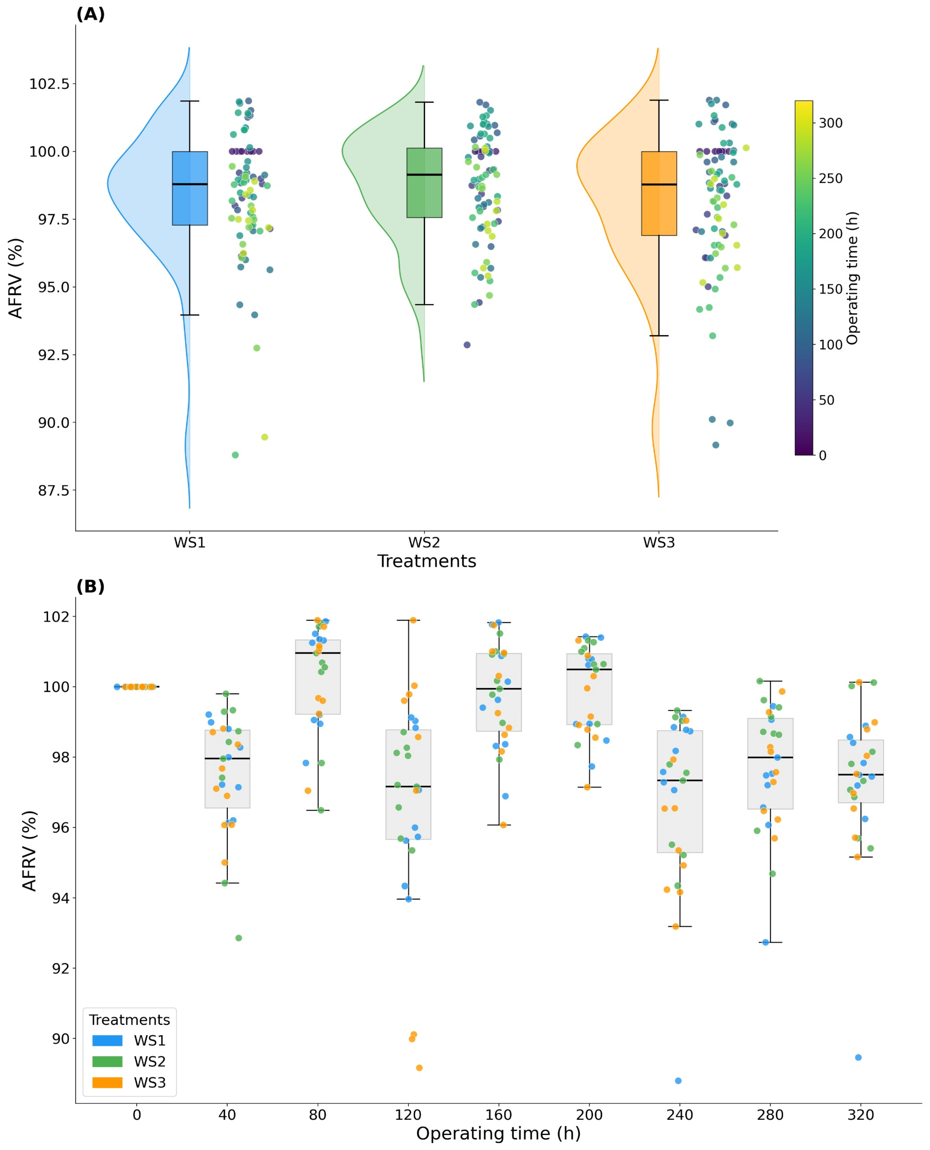
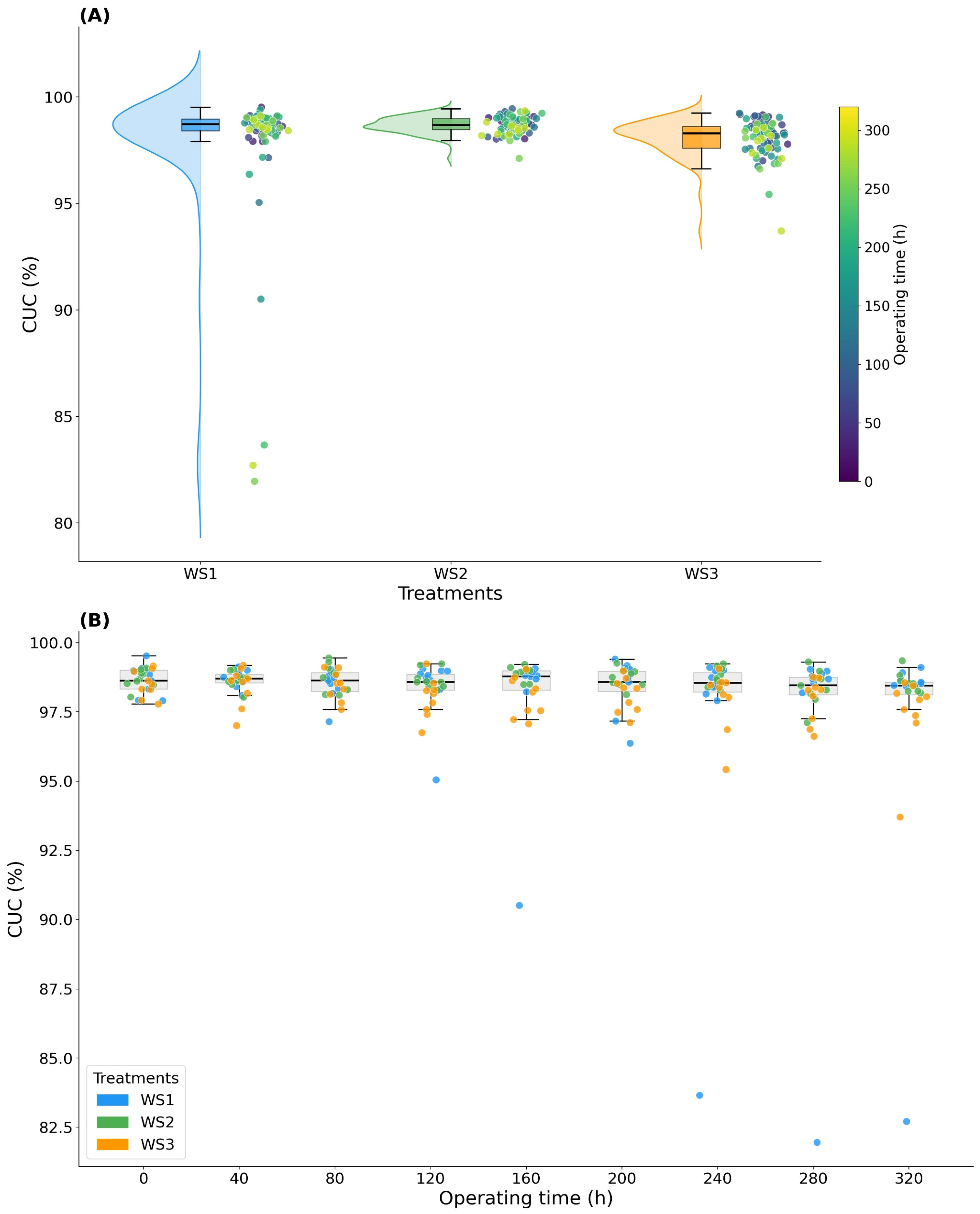
Figure 4 and Figure 5 show the temporal behavior of average flow-rate variation (AFRV) and Christiansen’s uniformity coefficient (CUC) for the three water sources, WS1, WS2, and WS3, considering the three drip-tape designs (D1, D2, and D3) operated in parallel over 0–320 h, respectively.

The distribution of AFRV as a function of water sources showed that the three treatments maintained high hydraulic performance throughout the 320 h of operation, with most values concentrated above 95%, probably due to the use of self-cleaning valves in all lateral lines. AFRV remained at high levels throughout the experiment, although with statistically significant temporal variation (Figure 4). When grouped by water source, the distributions showed very close central values, with medians ranging from 98.78 to 99.14%. WS2 had the highest median, at 99.14%, and comparatively lower dispersion (Q1 = 97.56% and Q3 = 100.12%), while WS1 and WS3 had slightly lower medians (98.79 and 98.78%, respectively) and greater dispersion, particularly WS3 (Q1 = 96.90% and Q3 = 100.00%). Occasional low AFRV events were observed for WS1 and WS3 (minimum = 88.79% and 89.17%, respectively), while WS2 exhibited a higher minimum (92.86%), suggesting a lower occurrence of severe reductions under WS2.

However, even in treatments with greater variability, the lowest observed values remained above the critical limit of AFRV < 75%, adopted as a reference for replacing lateral lines due to severe clogging. This result indicates that, at the end of the 320 h of operation, no treatment reached a critical hydraulic condition that would justify the immediate replacement of the lateral lines. The occurrence of minimum values close to 89% in WS1 and WS3 suggests the presence of localized flow reduction events, but without yet compromising the system at a critical level.

Regarding operating time, AFRV values generally remained high throughout the experiment (mostly around 96–101%); however, sharp reductions were observed, corresponding to clogging events. Visually, the most evident episodes occurred in WS2 at 40 h (an isolated drop, 93%), in WS3 at 120 h (the most severe cases, with values around 89–90%), and in WS1 at 240 h and 320 h (additional marked drops, 89–90%). Statistical analysis confirmed that these variations over time were significant, with the reduction in AFRV being more pronounced in specific treatment × time combinations. This temporal analysis shows that AFRV varied throughout the experimental period, with more evident fluctuations after 120 h of operation, especially in treatments containing saltworks bittern.

When grouped by dripper type, AFRV also remained high, but clear differences in stability were observed between emitters. D3 had the highest central value (median = 99.14%) and the lowest interquartile range (Q1 = 97.83% and Q3 = 100.00%), indicating greater uniformity. D2 had an intermediate median (98.64%) with moderate dispersion (Q1 = 97.19% and Q3 = 100.00%). In contrast, D1 exhibited the lowest median (98.78%) and the largest range (Q1 = 96.20% and Q3 = 100.00%), with the lowest minimum AFRV (88.79%), suggesting greater susceptibility to sporadic reductions in relative flow compared to D2 and D3.

These results suggest that the use of electronic pulses, combined with the presence of self-cleaning valves, may have contributed to mitigating the severity of critical flow reduction events, maintaining the AFRV at levels above the lateral line replacement limit. Although the treatment did not completely eliminate the hydraulic variability caused by saltworks bittern, its application appears to have favored the maintenance of the system’s operational performance. Thus, considering that the AFRV values remained above 75% after 320 h, it is possible to infer that the lateral lines still had potential for use for an additional period, potentially extending their lifespan and reducing maintenance costs, consumption of plastic materials, and environmental impacts associated with frequent pipe replacement.

The temporal oscillations observed in AFRV values may be associated with factors inherent to the operation of the benches under open-air conditions. Among these factors, possible random events of partial unblocking of the emitters stand out, resulting from the detachment of encrusting material accumulated inside the lateral lines, as well as small hydraulic disturbances caused by the movement of the pipes during performance evaluations. In addition, direct exposure to solar radiation and high temperatures during the hottest hours of the day may have promoted the expansion of the plastic material of the lateral lines and changes in water viscosity, temporarily influencing the flow rate of the emitters. Another relevant aspect refers to the intermittent operating regime, characterized by successive cycles of system activation and deactivation, which may favor internal rearrangements of the tanks and momentary variations in water flow along the lateral lines.

When grouped by water source, the median CUC ranged from 98.31% to 98.74% (Figure 5). WS1 showed the highest median, 98.74%, and a narrow interquartile range (Q1 = 98.42% and Q3 = 98.98%), but also the lowest minimum value, 81.96%, and the greatest variability (SD = 3.1871; CV = 3.25%), indicating sporadic but severe uniformity losses. WS2 exhibited a slightly lower median (98.69%) with very stable performance (Q1 = 98.48% and Q3 = 98.99%; SD = 0.396; CV = 0.40%) and a higher minimum (97.12%), suggesting less susceptibility to extreme deviations. WS3 presented an intermediate median (98.31%) and moderate variability (Q1 = 97.59% and Q3 = 98.62%; SD = 0.868; CV = 0.88%), with occasional reductions (minimum = 93.71%), but without the extremely low values observed for WS1.

Regarding operating time, CUC values remained consistently high throughout the experiment (mostly around 97.5–99.5%), indicating that irrigation uniformity was largely maintained over time, with reductions concentrated in specific events. Still, some low and isolated outliers were observed; The most pronounced reductions occurred in WS1, with a moderate drop at 120 h (95%), a larger drop at 160 h (90.5%), and the lowest values at 240 h, 280 h, and 320 h (approximately 82–84%), indicating recurrent hydraulic compromise in later stages of this treatment. In contrast, WS2 showed the most stable behavior, without marked low outliers, while WS3 remained mostly stable but exhibited occasional moderate reductions, particularly at 240 h (95%) and 320 h (94%).

When grouped by dripper type, the differences in stability became clearer. Group D3 achieved the highest median CUC (98.88%) and the most concentrated distribution (Q1 = 98.59% and Q3 = 99.08%; SD = 0.343; CV = 0.35%), with a high minimum (97.59%), indicating the most consistent uniformity. Group D2 presented an intermediate median (98.57%) and greater dispersion (Q1 = 98.13% and Q3 = 98.92%; SD = 0.899; CV = 0.91%), with occasional reductions (minimum = 93.71%). In contrast, D1 presented a median of 98.32% with a relatively narrow interquartile range (Q1 = 98.04% and Q3 = 98.64%), but the lowest minimum (81.96%) and the greatest variability (SD = 3.112; CV = 3.19%), indicating a greater propensity for sporadic and large-magnitude losses in uniformity. Overall, the results show that, although the typical CUC values were consistently high across treatments, the lower tail of the distributions, particularly for WS1 and D1, was determined by rare events that can substantially reduce irrigation uniformity.

3.4. Energy-Dispersive X-Ray Spectroscopy (EDS) Analyses, Scanning Electron Microscopy (SEM), and Fourier-Transform Infrared Spectroscopy (FTIR)

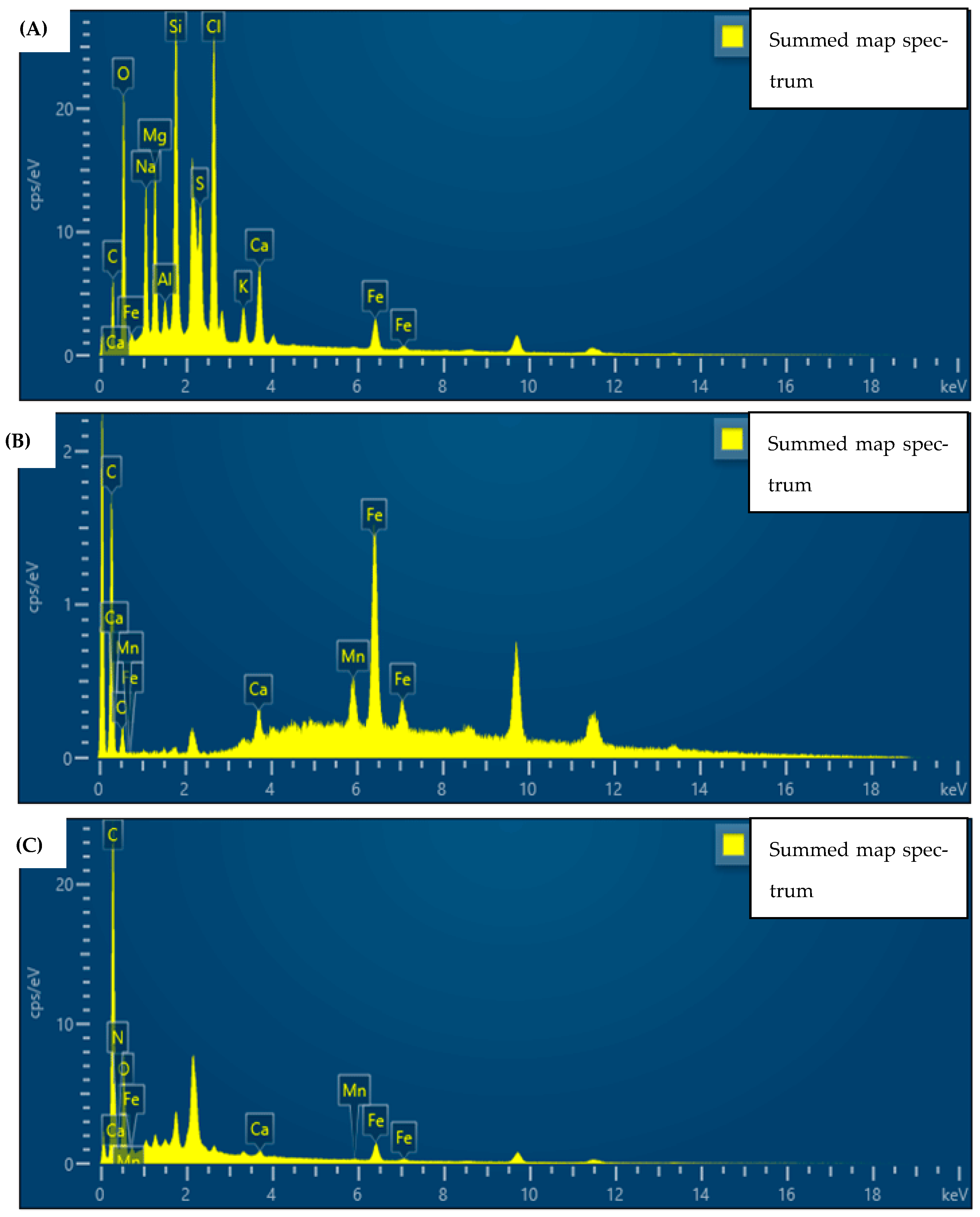
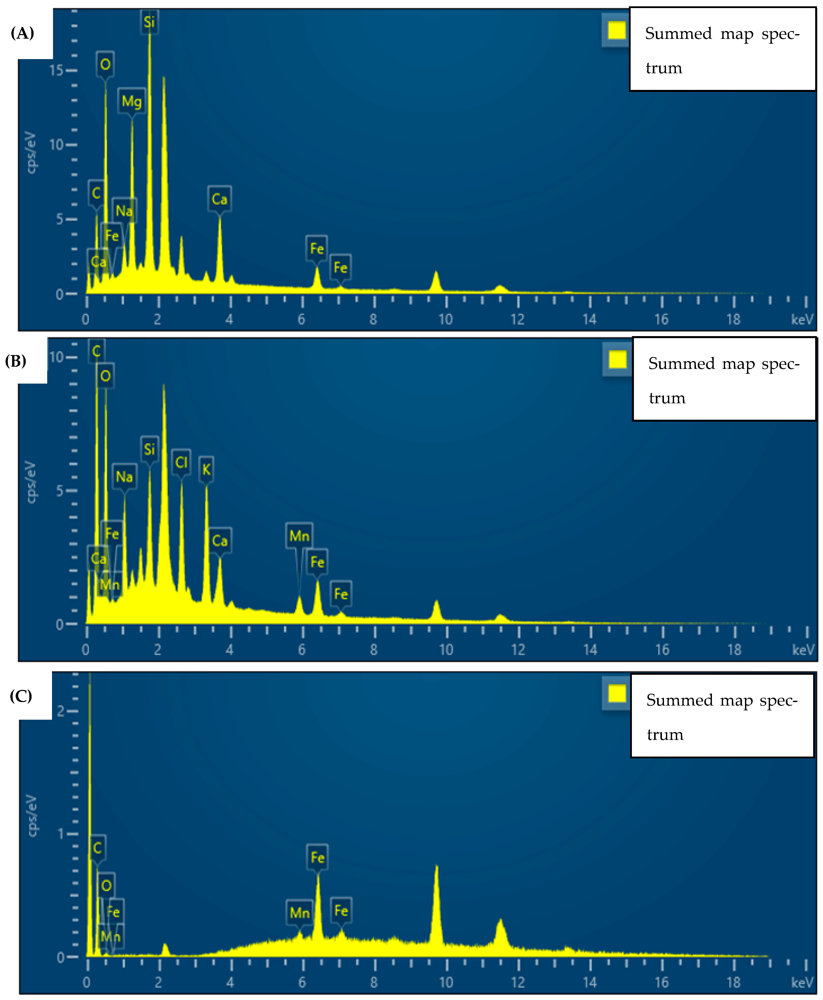
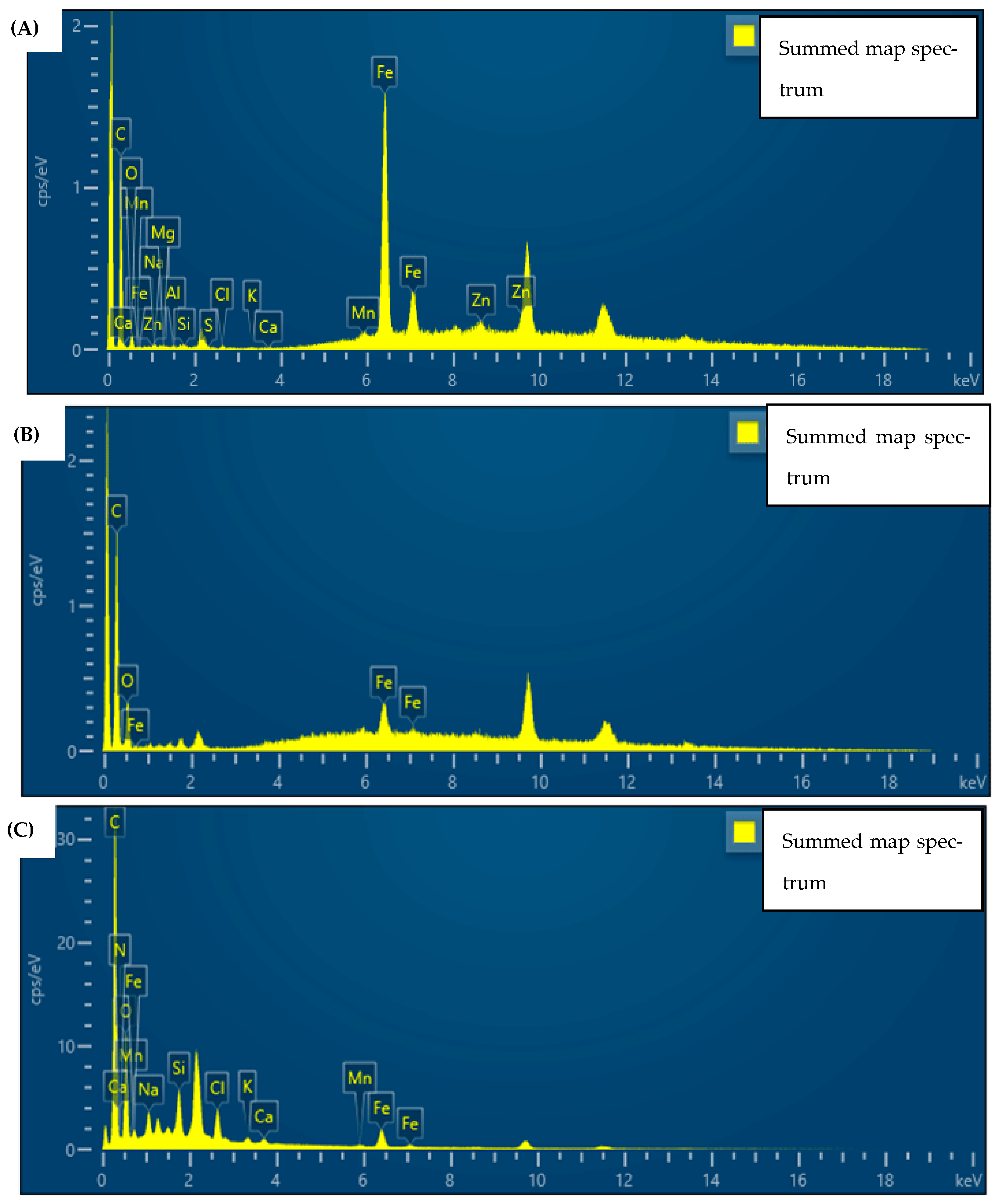
Figure 6, Figure 7 and Figure 8 present EDS spectrum of the deposits formed along the emitter labyrinths under the three water sources for each dripline model, D1, D2, and D3.

EDS results showed that deposit composition and spatial distribution varied with both water source and emitter design. Under WS1, deposit patterns were redistributed relative to WS3, without eliminating deposition. In D1 and D3, Fe-rich phases remained predominant at the inlet, but the inner labyrinth showed a reduced organic signal, and outlet deposits exhibited lower Ca and fewer Ca-enriched phases compared with WS3. In D2, inlet deposits also remained Fe-dominated, while the outlet showed lower Ca and reduced chemical complexity relative to WS3. Overall, D3 tended to confine mineral loading more to the outlet, D2 showed clearer propagation of mixed deposits along the labyrinth under WS3, and D1 showed the strongest and most persistent Fe/Mn retention from inlet to inner labyrinth across water sources.

Under WS2, all emitters exhibited deposits dominated by Fe/Mn rich phases at the labyrinth inlet, while Ca signals remained low, indicating no prominent Ca enriched deposits. In D3, the inner labyrinth showed low mineral loading and the outlet was dominated by Si—Al—Na—K particulates. In D2, the inner and outlet regions displayed more heterogeneous deposits composed mainly of fine particulates and salts (Si, Na, K, and Cl). In D1, Fe/Mn deposition at the inlet extended into the inner labyrinth, whereas the outlet contained more dilute, heterogeneous particulate/salt material with very low Ca.

With WS3, deposits became chemically more complex and extended further along the labyrinth. D3 showed Fe enrichment at the inlet, an increased organic/biological signal in the inner labyrinth (N detected), and outlet deposits combining Ca bearing phases, mineral particulates, and S-bearing compounds. D2 presented Fe retention at the inlet, organomineral signatures in the inner labyrinth with C associated with Fe/Mn, and enhanced Ca–Mg–Si signals at the outlet, consistent with carbonate- and silicate-associated material. D1 displayed organomineral signatures within the labyrinth with elevated C and N associated with Fe, and outlet deposits enriched in Si–Al–Mg, while Ca remained comparatively low.

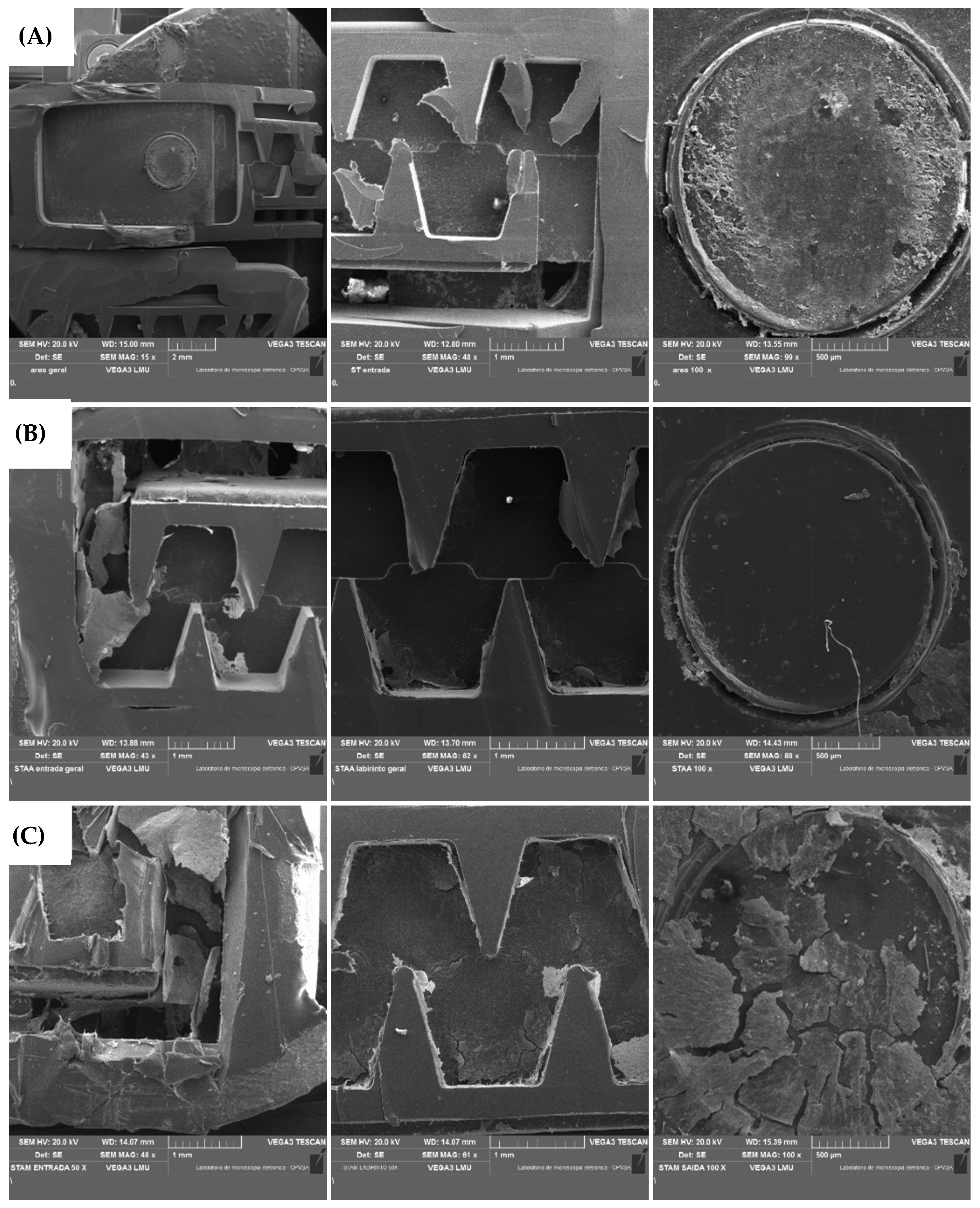
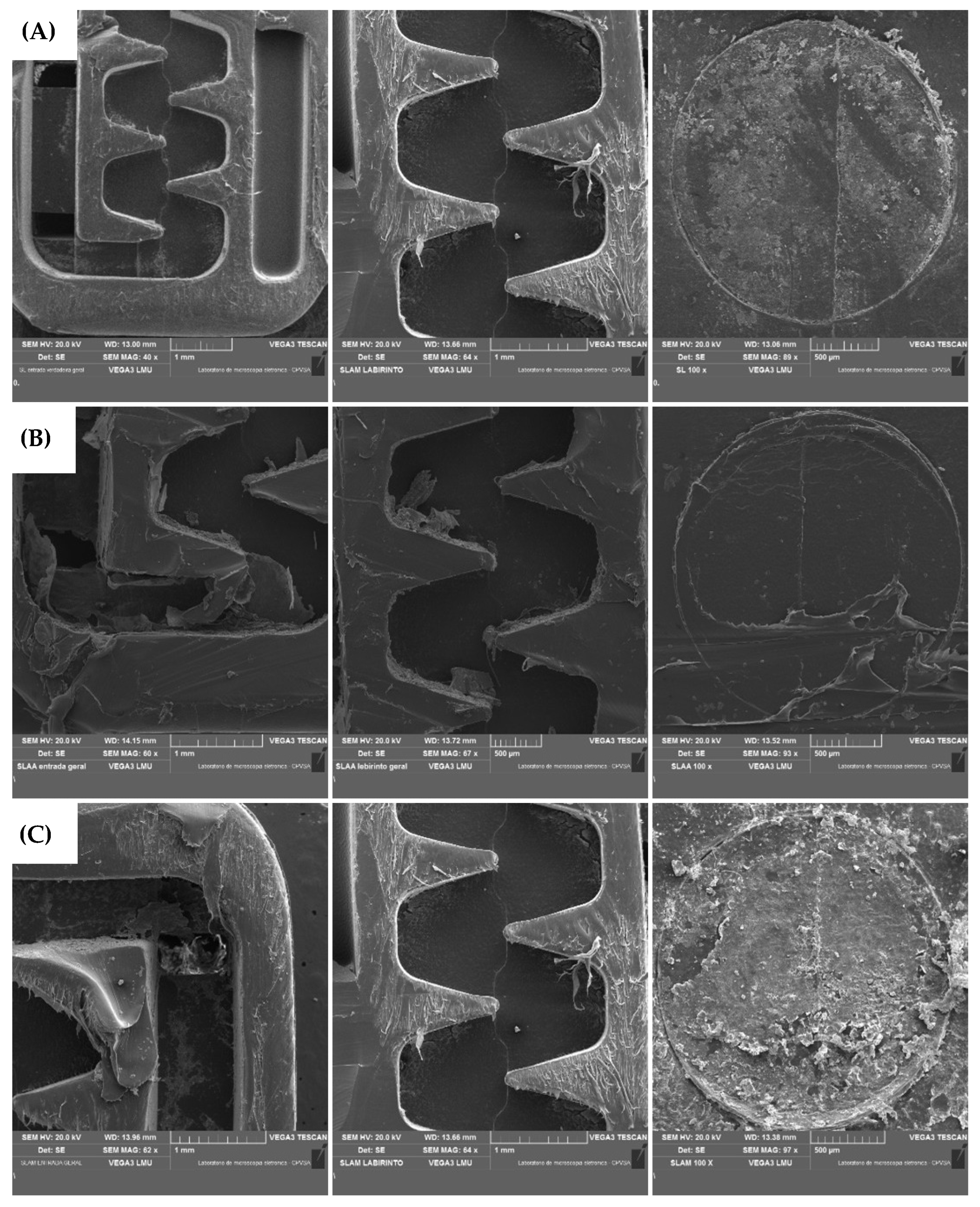
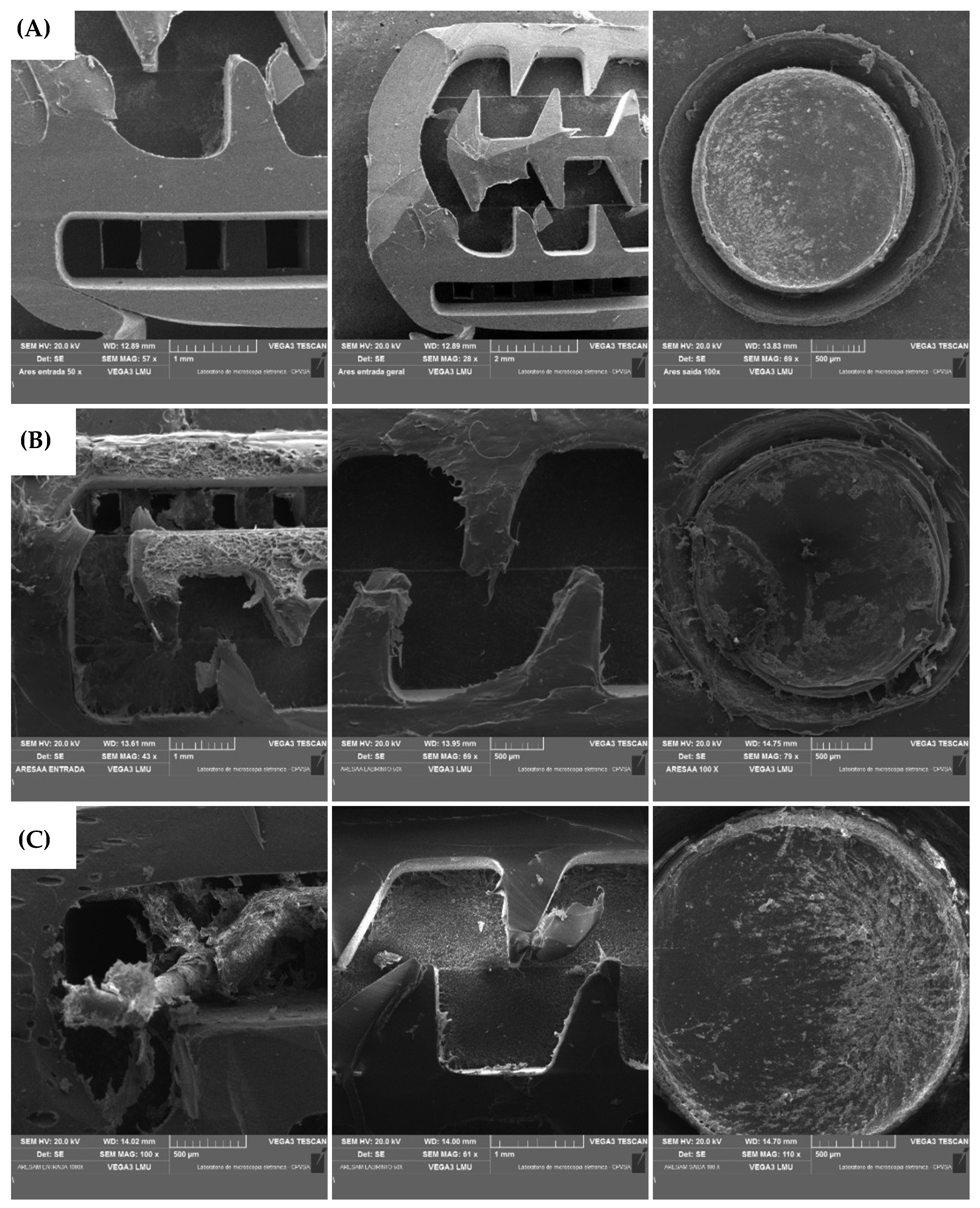
Figure 9, Figure 10 and Figure 11 present SEM micrographs of the deposits formed along the emitter labyrinths under the three water sources for each dripline model, D1, D2, and D3.

SEM images showed that deposit distribution along the labyrinth depended strongly on water type across the three emitters. Under WS2, all emitters exhibited a predominantly localized deposition pattern, with deposits concentrated mainly at the inlet and visibly reduced accumulation along the inner labyrinth and toward the outlet. Under WS3, deposit coverage increased markedly, with more continuous and thicker layers extending through the labyrinth and a pronounced accumulation at the outlet, indicating a more extensive deposition pattern relative to WS2. For WS1, the SEM images indicated a redistribution of deposits compared with WS3, characterized by reduced evidence of continuous deposits within the labyrinth and a more discontinuous, particulate-dominated pattern, with less pronounced outlet accumulation than under WS3.

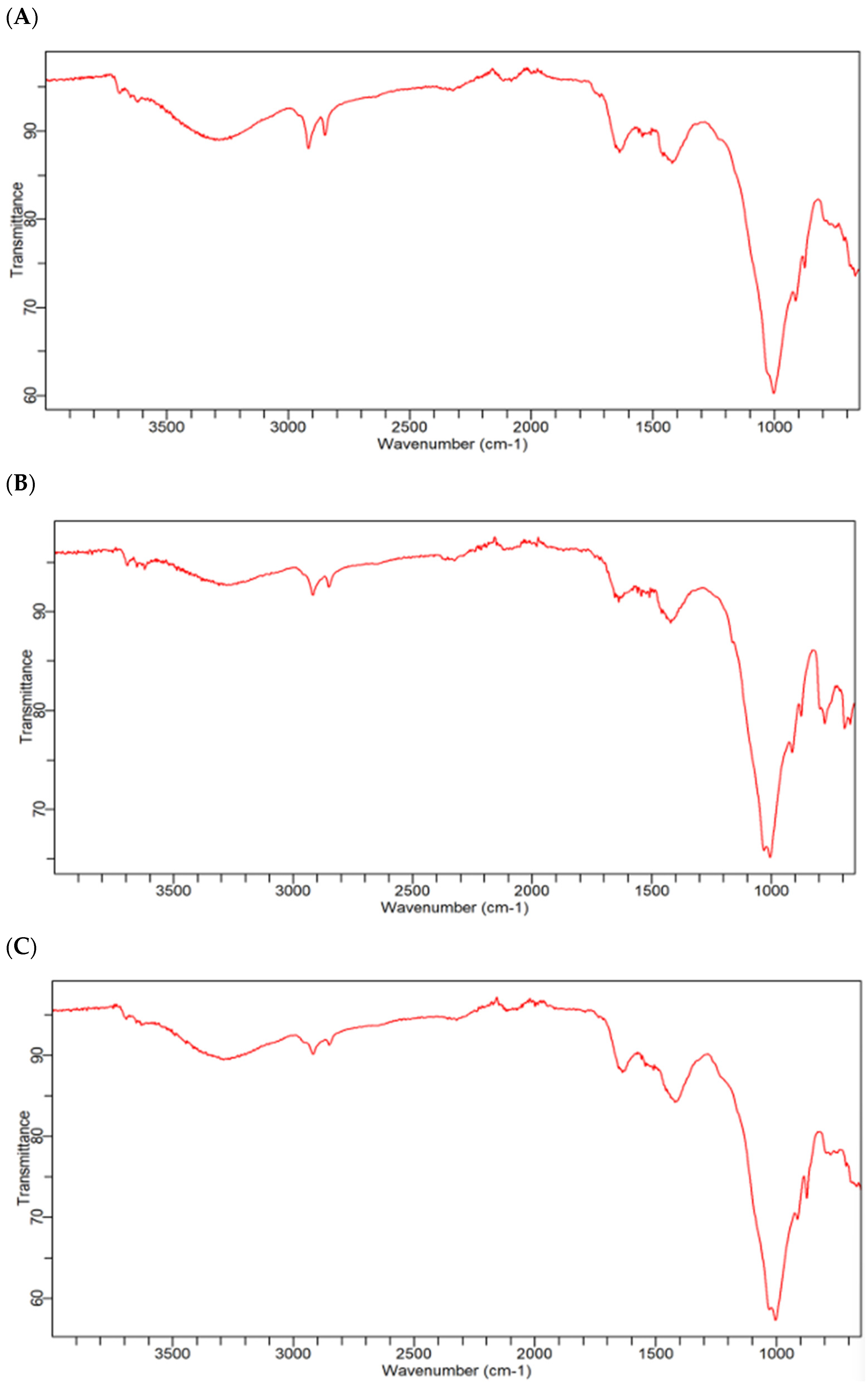
The FTIR spectra of the composite samples WS1, WS2, and WS3 (Figure 12), obtained in the range of 4000–650 cm⁻¹, with 24 scans, a resolution of 4 cm⁻¹, and an operational status of the system classified as good, indicated the presence of functional groups compatible with an organomineral matrix.

4. Discussion

4.1. Effect of Water Quality on Emitter Clogging

WT showed a small but statistically significant difference among water sources (p = 0.0319), with close medians and largely overlapping interquartile ranges. This overall stability is consistent with a recirculating bench experiment in which WT is mainly governed by the system heat balance, ambient conditions (air temperature, radiation, ventilation), heat exchange in reservoirs and pipelines, and the operating schedule, rather than by water origin alone. Even with statistical significance, the absolute separation was small: WS1 remained only slightly warmer than WS3 (about 0.8 °C), which could be compatible with additional heat dissipation from the electromagnetic pulse device via Joule heating in an electrically conductive solution. However, given the strong distribution overlap and the sensitivity of open recirculating benches to day-to-day microclimatic variability, this contribution cannot be isolated from environmental drivers [53,75,76].

Importantly, the observed WT range still matters because it sets the background conditions for clogging, even if it only weakly discriminates treatments. Temperature influences water viscosity and therefore emitter hydraulics, affecting low-velocity zones where suspended particles and precipitates preferentially accumulate, and it can also modulate reaction kinetics and carbonate equilibria that control inorganic scaling under alkaline, saline conditions. In addition, temperatures around 30–32 °C are compatible with microbial activity, which may favor biofilm development when nutrients and attachment sites are available, thereby reinforcing mixed clogging processes when particulates and mineral precipitation occur simultaneously [36,77,78].

In contrast, TSS clearly discriminated the control water from the bittern waters: WS2 presented null values, when both WS1 and WS3 exhibited higher and similar concentrations (10 and 12 mg L⁻¹). As observed, all median levels were less than 200 mg L⁻¹ across the three water sources, indicating low emitter clogging risk [64]. TSS is an essential driver of physical clogging through particle deposition within low-velocity regions of the emitter’s labyrinth, and it also promotes coupled clogging by providing surfaces for heterogeneous nucleation of mineral precipitates and for microbial attachment [76,79,80]. Although WS1 and WS3 remained statistically similar for TSS, the 16.7% lower median in the EP-treated bittern suggests a potentially lower particulate load reaching the emitters, which may reduce the cumulative rate of deposition and the availability of nucleation/attachment sites over operating time, effects that are especially relevant in narrow hydraulic pathways typical of drip irrigation.

pH differed significantly among water sources (p < 0.0001), with the control water WS2 exhibiting a higher median pH of 8.95 than WS1 and WS3 (medians 8.74 and 8.68, respectively), and with WS1 and WS3 remaining in the same statistical group. This separation likely reflects differences in carbonate alkalinity control and conditioning: WS2 typically has pH stabilized by drinking-water treatment practices, whereas bittern waters are dominated by concentrated salts and carbonate equilibria that can shift with recirculation, evaporation, and gas exchange with the atmosphere [35,58]. The fact that WS1 and WS3 were statistically similar indicates that the electromagnetic pulse treatment did not consistently modify bulk pH at the scale of the experiment, despite the slightly higher median observed in WS1. The observed pH range (approximately 8.7—9.0) across the three water sources remains critical for drip irrigation and indicates a severe risk of dripper clogging (pH > 8) [65]. Under alkaline conditions, a larger fraction of dissolved inorganic carbon occurs as CO₃²⁻, which increases the likelihood of Ca-Mg carbonate precipitation when Ca²⁺/Mg²⁺ are available and when local supersaturation develops within emitter labyrinth microenvironments [76,81]. pH also influences surface charge and interfacial interactions, affecting crystal nucleation and adhesion to polymeric walls and favoring mixed deposits when suspended particles and biofilm matrices are present [82]. However, clogging risk is not governed by pH alone; it results from the combined effect of pH with salinity/ionic strength, hardness ions, and particulate load. In this context, although WS2 exhibited the highest pH, WS1 and WS3 remain more chemically prone to deposition and clogging when considered alongside their broader physicochemical profile, while differences between WS1 and WS3 are more plausibly linked to deposition/adhesion dynamics than to bulk pH shifts.

WS1 and WS3 exhibited elevated and statistically similar median EC values (2.97 and 2.78 dS m⁻¹, respectively), whereas the control water WS2 showed a substantially lower (0.58 dS m⁻¹). This pattern is consistent with the higher dissolved salt load of bittern relative to treated supply water and represents low tendency to clogging for WS2 and moderate risk for WS1 and WS3 [64]. Because WS1 and WS3 share the same origin, the lack of a significant difference indicates that the electromagnetic pulse treatment did not measurably change bulk salinity and any small shifts in central tendency are more plausibly linked to bench operation (recirculation, evaporation, and water replacement) than to direct chemical alteration of ionic content. High EC is a practical indicator of increased ionic strength and a greater propensity for local supersaturation and precipitation when combined with alkaline pH and hardness ions (Ca²⁺/Mg²⁺), thereby elevating the risk of inorganic scaling within emitter labyrinths. Elevated salinity can also reduce electrostatic repulsion, promote particle aggregation and enhancing the adhesion of colloids and crystals to polymeric surfaces, which favors mixed deposits and progressive flow restriction [38]. In contrast, the lower EC in WS2 implies reduced salinity stress and soil-salinization risk, and typically a lower chemical load contribution to clogging, whereas the higher EC of bittern waters requires careful management and has direct hydraulic implications for clogging development and distribution uniformity. Since EC does not differentiate WS1 and WS3, any treatment related differences in hydraulic performance are more likely attributable to deposition/adhesion dynamics (e.g., suspended solids behavior, nucleation/aggregation, and deposit cohesion) than to changes in overall salinity.

Ca²⁺ and Mg²⁺ differed strongly among water sources, with a clear separation across the water sources. WS2 showed lower concentrations of median Ca²⁺ and Mg²⁺ (10 mg L⁻¹ and 3.96 mg L⁻¹, respectively), in contrast with WS1 and WS2 with elevated medians of Ca²⁺ (48 and 47.2 mg L⁻¹, respectively) and Mg²⁺ (146.4 and 168 mg L⁻¹, respectively). This contrast is consistent with water origin, bittern is a concentrated saline effluent enriched in divalent ions, whereas treated supply water typically has low hardness. Importantly, the absence of a significant difference between WS1 and WS3 indicates that the ultra-low-frequency pulse treatment did not measurably reduce bulk hardness, which is expected for electromagnetic approaches.

From a clogging perspective, the elevated Ca²⁺ and Mg²⁺ in the bittern waters directly increase the potential for chemical clogging by promoting precipitation and deposition, particularly as carbonates under alkaline and saline conditions. WS1, WS2 and WS3 presented minor risk of clogging from Ca levels, and severe risk from Mg concentrations [64]. In drip emitters, the labyrinth’s low-velocity zones and constrictions favor heterogeneous nucleation and crystal growth on internal polymer surfaces; once an initial mineral layer forms, surface roughness and interfacial energy tend to enhance further scaling and improve deposit persistence. Mg²⁺ is also relevant because it can alter CaCO₃ crystallization kinetics and polymorphism, potentially changing deposit texture and adhesion strength. High divalent-ion loads contribute to salinity and cation balance concerns in the soil water system, but hydraulically the most immediate implication is that, when coupled with the elevated EC and alkaline pH already observed for the bittern waters, high hardness intensifies the likelihood of inorganic scaling and mixed deposits, accelerating discharge reduction and compromising uniformity over time. Because Ca²⁺ and Mg²⁺ do not differentiate WS1 and WS3, any treatment-related differences in hydraulic performance are more likely to arise from changes in deposition/adhesion behavior (e.g., particle–crystal interactions, nucleation on surfaces, and deposit cohesiveness) rather than from changes in bulk Ca²⁺/Mg²⁺ concentrations [83,84,85,86].

Fe and Mn mean concentrations remained far below the minimum thresholds (0.5 and 0.7 mg L⁻¹, respectively) used to classify the chemical risk of dripper clogging [64]. The slightly different statistical suggests that, in a global sense, water source contributed to variability in these metals, with a small to moderate effect sizes and substantial overlap among distributions, where the dataset is heterogeneous enough to yield a significant F-test, yet not consistent enough (or not sufficiently separated) to produce clear pairwise separation. Fe and Mn are critical because they can shift oxidation state and precipitate as insoluble oxides/hydroxides (or form mixed organomineral phases), particularly under alkaline conditions, in the presence of dissolved oxygen. It may also be associated with biofilm growth, favoring mixed bio-mineral deposits and emitter obstruction [52,87].

Overall, the electromagnetic pulse treatment did not alter the bitterns’ physicochemical properties, as WS1 and WS3 remained statistically similar for the main indicators of salinity and hardness (EC, Ca²⁺, and Mg²⁺) and pH, WT, Fe, and Mn. This outcome is consistent with the expected mechanism of the treatment, which is not designed to remove dissolved ions or substantially shift equilibrium chemistry at the system scale. Instead, the clearest treatment-related tendency was observed for TSS, where WS1 showed a lower median than WS3, suggesting a potential reduction in the particulate load reaching the emitters and, consequently, fewer surfaces for heterogeneous nucleation and biofilm assisted deposition.

4.2. Hydraulic Performance and Dripper Clogging Mitigation Under Electronic Pulses

AFRV reflects deviations in median discharge relative to baseline, thus responding to global or localized flow restriction events. CUC translate these variations into practical uniformity terms, while CUC is sensitive to overall dispersion across the field/bench, In clogging evolution, it is common to observe that CUC may remain relatively high until clogging becomes more widespread, while AFRV can show transient dips if restriction events occur and later partially reverse due to deposit sloughing, pressure fluctuations, or particle redistribution in recirculating systems.

Across the 0 to 320 h operating period, all water sources sustained generally high AFRV and CUC in typical conditions, but clear differences emerged by occurrence and severity of clogging. WS2 behaved as the most stable condition, with tight distributions and no evidence of severe discharge or uniformity losses, consistent with a lower clogging potential and fewer transient loading events. In contrast, the same alternative source used in WS1, when applied without electronic pulses (WS3), showed the greatest hydraulic oscillation, including deeper low-end AFRV events and more frequent departures from the main performance band, behavior compatible with episodic restriction events driven by particulates and/or mixed deposits. WS1 tended to mitigate the most damaging deviations relative to WS3, indicating that treatment acted primarily by reducing the severity and/or persistence of clogging rather than by shifting the typical central performance.

AFRV remained near nominal values in most cases, but the untreated alternative source (WS3) exhibited the clearest signatures of transient discharge reductions, especially when paired with the most sensitive dripper design (D1). In this configuration, AFRV reached sharp low-end events close to 89%, which is consistent with a short-term restriction episode rather than gradual uniform deterioration. Such events are plausible under untreated water because suspended solids and unstable aggregates can episodically accumulate at constrictions or low-velocity pockets of the emitter labyrinth. Mixed deposits can contribute to a nonlinearly behave once a critical threshold is reached, head loss increases abruptly and flow rate decreases; later, shear forces, pressure fluctuations, or partial detachment can reopen the pathway, producing the drop and recover behavior suggested by the AFRV time distribution. By contrast, the control water from the supply company (WS2) showed tightly clustered AFRV values and a higher minimum, which supports the interpretation that its small oscillations reflect operational variability (pump cycling, minor pressure variation, measurement noise) rather than clogging. The treated version of the alternative source (WS1) generally reduced the severity and/or persistence of the most damaging AFRV departures relative to WS3, indicating that treatment acted as a mitigation step by limiting the processes that convert transient loading into hydraulically meaningful deposits, even if typical discharge remained close to nominal.

CUC likewise remained high (around 98 a 99%) in most cases, and it indicates that within the tested duration the dominant regime was incipient to moderate clogging, with strong impacts concentrated in specific water design combinations. CUC is an aggregate uniformity metric and can remain high when only a small fraction of emitters is affected or when deviations are modest; however, it drops sharply when a few emitters become severely restricted because it is highly sensitive to spatial heterogeneity. This explains why WS1 could maintain high typical CUC while still exhibiting rare severe minima: the overall network remained near-uniform most of the time, but occasional few emitter failures produced disproportionate reductions in uniformity. In contrast, WS2 presented stable CUC without extreme excursions, consistent with a low driving force for heterogeneous deposit formation. WS3 showed greater vulnerability than control, aligning with the expectation that untreated water increases the probability of localized clogging and heterogeneous discharge patterns.

Once the treatment effect is interpreted as conditional on emitter design, D1 emerges as the most sensitive configuration, showing the strongest low-end behavior in both AFRV and CUC. This sensitivity can be attributed to hydraulic pathway features that favor particle capture and deposit maturation such as narrower critical sections, sharper contraction/expansion transitions, or internal niches where velocity is low enough to allow settling and attachment. Once initial retention occurs, subsequent accumulation becomes self-reinforcing: roughened surfaces and early deposits increase effective attachment area for particulates and organomineral matrix, and these matrices can then stabilize mineral precipitates, increasing deposit cohesion and persistence. By contrast, D3 appeared more resilient, maintaining stable AFRV and CUC with fewer extreme departures, implying a geometry that either reduces capture probability or promotes self-flushing through sustained turbulence and fewer stagnation zones. This design dependence is central to the interpretation of the treatment: mitigation is most visible in sensitive designs because small reductions in deposition efficiency (less available particulate matter, weaker adhesion, or less cohesive deposit texture) can delay threshold bridging and suppress the extreme lower tail that drives performance risk. In robust designs, differences are naturally less pronounced because the emitter already resists clogging under the tested conditions.

Taken together, the water-source ordering supports a coherent clogging narrative. WS2 represents a low clogging-risk baseline, consistent with stable AFRV and CUC and the absence of severe uniformity collapses and TSS = 0 and low EC/hardness. WS3 represents elevated mixed-deposition risk, expressed not necessarily as lower typical performance but as a higher probability of transient, high-impact restriction events, particularly in sensitive emitters. The treated WS1 sits between these conditions, behaving closer to control in terms of tail risk while still sharing the same source origin as WS3. This pattern aligns with a mitigation mechanism in which treatment does not need to dramatically shift medians to be operationally valuable; instead, its key benefit is suppressing rare failures (deep AFRV dips and sharp CUC collapses) that dominate long-term reliability and agronomic consequences.

The treatment applied in WS1 likely provided partial mitigation, a performance buffer, rather than a complete removal of clogging risk. It reduced the conversion of transient loading into persistent heterogeneous obstruction, but it did not eliminate the possibility of episodic restrictions, especially in sensitive emitter designs. Therefore, the most defensible engineering interpretation is that water treatment and emitter selection must be treated as coupled controls. A resilient labyrinth (as suggested by D3) reduces sensitivity to water quality variability, while a more sensitive design (D1) amplifies tail risk and may require stronger mitigation measures (more robust filtration, adaptive flushing, and, where appropriate, additional conditioning) to maintain discharge and uniformity when operating with alternative waters. This framing matches the observed data structure: typical AFRV and CUC remained high across conditions, but the reliability of performance, expressed in the lower tail, was governed by the interaction between source water quality (treated vs. untreated) and emitter design sensitivity.

Based on the water-quality profile and hydraulic response, WS2 represents low clogging risk, consistent with TSS = 0 and low EC/hardness. The observed AFRV oscillations are better interpreted as operational variability rather than sustained clogging. The bittern waters (WS1 and WS3) represent elevated chemical and mixed deposition risk because they combine high ionic strength with high Ca²⁺/Mg²⁺ under alkaline pH, plus a measurable particulate load that enables heterogeneous nucleation and organomineral matrix attachment. However, the hydraulic indicators suggest that, within 320 h, clogging was moderate overall, with the most concerning pattern being the WS1/D1 combination. In practical terms, that configuration is trending toward a level where nonuniform irrigation and maintenance needs become significant, especially for saline irrigation strategies where uniformity protects crops and mitigates salt accumulation.

The combined evidence supports a nuanced conclusion: EP treatment did not change bulk salinity or hardness, consistent with the water-quality results, but it likely influenced the processes that convert water quality into deposits. The modest reduction in TSS median in WS1 compared with WS3 suggests lower particulate availability to seed deposits, and the hydraulic data indicate that WS1 generally avoided the strongest deterioration observed under WS3, particularly for the most sensitive tape design (D1). This pattern aligns with a mitigation mechanism in which electronic pulses reduce effective particle adhesion, modify aggregation behavior, or shift crystallization/adhesion dynamics so that deposits either form less efficiently, remain less cohesive, or detach more readily under shear.

At the same time, EP did not eliminate clogging risk under bittern because the primary thermodynamic drivers for scaling (high EC and high Ca²⁺/Mg²⁺ under alkaline pH) remained present. Therefore, the most defensible interpretation is that EP treatment provided partial mitigation, a performance buffer, rather than a complete solution. In engineering practice, that means EP could be valuable as part of an integrated strategy (filtration, chemical conditioning when appropriate, hydraulic design selection, and maintenance flushing), particularly when the system must operate with saline effluents such as bittern. The tape design dependence observed here reinforces that emitter selection is as important as water treatment: a resilient labyrinth (D3) can reduce sensitivity to harsh water, while a more sensitive design (D1) may require stronger mitigation measures to maintain uniformity and avoid progressive clogging under untreated bittern.

In summary, the hydraulic indicators and water quality data converge on a consistent narrative: WS3 increased the likelihood of mixed deposits and heterogeneous clogging, while the EP treated bittern (WS1) maintained performance closer to the control by moderating the deposition pathway rather than altering bulk chemistry. This supports the proposed topic framing that electronic pulses can mitigate clogging development, but their benefit is conditional on emitter design and does not replace the need for broader salinity and scaling management when irrigating with concentrated saline effluents.

4.3. SEM–EDS and FTIR Analyses of Deposit Morphology, Elemental Composition, and Functional Groups

EDS analysis of deposits in the D1 emitter also revealed important variations in the nature and spatial distribution of deposits. With WS2, intense retention of Fe and Mn was observed at the labyrinth inlet, with propagation of these deposits into the inner section, characterizing a continuous iron-based clogging pattern, while the outlet concentrated more diluted and heterogeneous deposits formed by fine particulate material and salts, with very low Ca contents, ruling out relevant carbonate scaling.

Under WS3, clogging became more complex, with the formation of organomineral deposits within the labyrinth, evidenced by elevated contents of C and N associated with Fe, and with the accumulation of silicates and mineral particles (Si, Al, Mg) at the outlet, indicating a mixed clogging mechanism involving metallic, organic, and mineral components, although carbonate participation remained secondary.

In turn, the use of EP in WS1 promoted redistribution of deposits, maintaining the predominance of iron-rich phases at the inlet, but reducing the organic contribution within the labyrinth and forming more homogeneous mineral deposits at the outlet, with lower Ca contents and the absence of pronounced carbonate scaling compared with WS3.

EDS analysis of deposits in the D2 emitter also showed that water quality directly influenced both clogging mechanisms and the spatial distribution of deposits along the labyrinth. With WS2 deposition at the labyrinth inlet was predominantly associated with iron- and manganese-bearing compounds, whereas the inner section and outlet presented more heterogeneous deposits, formed by fine particulate material and salts (Si, Na, K, and Cl), with low Ca contents, indicating the absence of dominant carbonate scaling.

With WS3, there was a significant increase in the chemical complexity of deposits, characterized by Fe retention at the inlet, formation of organomineral deposits rich in C/Fe/Mn within the labyrinth, and accumulation of carbonates and silicates (Ca, Mg, and Si) at the outlet, configuring a mixed clogging scenario involving physical, chemical, and organomineral mechanisms.

In turn, operation with EP in WS1 promoted a redistribution of deposits, with predominance of iron rich phases at the inlet and a relative reduction in chemical complexity at the outlet, as well as lower Ca contents compared with WS3. This suggests that magnetization altered precipitation and adhesion processes, attenuating carbonate scaling and the formation of more complex deposits, particularly at the labyrinth outlet. Overall, the results indicate that the D2 emitter is highly sensitive to water quality: poorer-quality waters intensified and diversified clogging mechanisms, whereas magnetization acted as a partial mitigating factor by modifying the nature and location of deposits along the labyrinth.

EDS characterization of the deposits formed in the WS3 emitter showed that water type influenced both the composition and the location of deposits along the labyrinth. Under WS2, deposits associated with iron and manganese bearing compounds were observed at the labyrinth inlet, while the inner section showed a low mineral load, and the outlet concentrated particulate material rich in Si, Al, Na, and K, with reduced Ca contents, indicating the absence of dominant carbonate scaling.

Under WS3, a marked increase in deposit complexity was observed, characterized by high Fe at the inlet, followed by a predominance of organic/biological material inside the labyrinth (presence of N), and culminating at the outlet with the simultaneous accumulation of carbonates (Ca), mineral particles, and sulfur-bearing compounds. This pattern indicates the coexistence and superposition of physical, chemical, and biological clogging mechanisms, associated with poorer water quality.

In turn, the use of EP in WS1 resulted in a redistribution of deposits, with preferential retention of iron-rich phases within the labyrinth, an evident reduction in organic matter, and lower Ca contents at the outlet compared with the WS3 treatment. These results suggest that EP did not eliminate deposit formation, but altered precipitation and adhesion processes, reducing chemical complexity and carbonate and biological scaling in critical regions of the emitter.

A comparative analysis of the EDS results showed that clogging mechanisms in drippers are strongly dependent on the emitter’s internal geometry, in addition to the quality of the applied water. The D3 emitter exhibited relatively more balanced behavior, with predominantly iron based deposits at the inlet, low mineral accumulation within the labyrinth, and mixed deposits at the outlet only when operated with poorer-quality water. This pattern indicates a greater capacity to confine deposits to specific regions, which may contribute to improved overall anti-clogging performance.

The D2 emitter showed Fe/Mn retention at the inlet, formation of organomineral deposits within the labyrinth when operated with bittern water, and accumulation of carbonates and silicates at the outlet, evidencing a greater propagation of clogging mechanisms along the channel compared with D3.

In turn, the D1 emitter exhibited strong and persistent deposition of Fe and Mn from the inlet to the inner section of the labyrinth, regardless of water quality, with worsening clogging mechanisms under bittern water. Even under magnetized bittern water, the dominance of iron-rich deposits was maintained, indicating a high affinity of this emitter geometry for the retention of metallic compounds. Overall, the results demonstrate that clogging resistance depends not only on water quality, but primarily on the interaction between chemical composition, local hydrodynamics, and labyrinth geometry.

Figure 9, Figure 10 and Figure 11 reveal significant differences in deposit formation along the labyrinth depending on the quality of the water used. Under WS2, SEM images show predominantly localized accumulation of deposits at the emitter inlet, transitioning to regions with fewer deposits in the inner labyrinth and at the outlet, characterizing a more localized and less extensive deposition pattern. This pattern was corroborated by EDS analysis, which indicated higher concentrations of Fe and Mn at the inlet, whereas the outlet exhibited finer, particulate deposits dominated by silicates (Si, Al, Na, and K) and low Ca contents, suggesting the presence of ferruginous compounds under AA without significant calcium carbonate formation.

In contrast, under the WS3, SEM images evidenced a marked increase in the extent and continuity of deposits, with thicker and more diffuse layers forming within the labyrinth and pronounced accumulation at the outlet. This observation was supported by EDS data indicating greater chemical complexity, with elevated Fe at the inlet, the presence of organic matter (N) within the labyrinth, and accumulation of carbonates (Ca) and mineral particles (Si, Mg, and Al) at the outlet. These findings suggest that the poorer water quality favored mixed clogging mechanisms involving biological, organic, and mineral processes, including the formation of carbonates and silicates.

Finally, under WS1, SEM images indicated a redistribution of deposits, with less evidence of continuous accumulation of organic material within the labyrinth and a greater predominance of particulate mineral deposits. EDS analysis showed that, despite presenting a pattern like WS3 in terms of Fe retention, water magnetization significantly reduced the contribution of organic matter and carbonates (Ca) at the outlet, resulting in more homogeneous and less complex deposits. This redistribution of deposits can be attributed to water magnetization, which altered the precipitation and adhesion dynamics of compounds within the emitter.

These results demonstrate that, whereas supply water produced more localized deposits dominated by Fe/Mn, bittern water promoted more extensive and diversified clogging with a stronger contribution of biological and carbonate related processes, and magnetized bittern acted as a mitigating factor by reducing deposit complexity, particularly at the emitter outlet. Overall, these findings suggest that water magnetization may be a useful strategy to control the formation of more complex obstructions.

The deposition patterns observed under WS1, WS2, and WS3 are consistent with the results reported by [53], who demonstrated that water quality and the application of physical treatments directly influence the nature and intensity of scaling. As described by those authors, emitters operating with supply water (WS3/WS2) presented relatively clean surfaces, with localized and weakly cohesive deposits, consistent with better hydraulic performance. Drippers applying untreated produced water exhibited extensive scaling layers formed by crystalline agglomerates and adhered particulate material, as well as dense biofilm, which explained the greater decline in hydraulic performance over time. In turn, emitters subjected to produced water treated with electronic pulses showed fewer and less cohesive deposits, with smaller crystals and modified morphology, distributed more sparsely along the labyrinth [53]. Other studies have also reported that water magnetization modifies the morphological structure of deposits [88,89].

The FTIR spectra of deposits collected under WS1, WS2, and WS3 (Figure 12) showed similar spectral profiles, indicating that the clogging material had a comparable chemical nature among the three water sources. In all spectra, broad absorption bands around 3200–3400 cm⁻¹ suggest the presence of O–H groups, which may be associated with adsorbed water, hydroxylated minerals, or organic compounds. Bands near 2900 cm⁻¹ indicate C–H vibrations, suggesting the occurrence of organic material in the deposits. The intense bands observed between approximately 1000 and 1100 cm⁻¹, together with bands in the 1400–1600 cm⁻¹ region, indicate the presence of mineral components, possibly associated with carbonate, silicate, or other oxygenated inorganic groups. Overall, the FTIR results suggest that the deposits formed in the emitters consisted of a heterogeneous organomineral matrix, with both inorganic precipitates and organic-associated material.

The mitigation of clogging by electronic pulses is attributed to physical alterations in the crystallization and deposition dynamics of distributed and suspended constituents in freshwater with a dose of saltworks bittern. Electronic pulses with a frequency range of 3–32 kHz are transmitted through the tube wall, promoting the formation of suspended microcrystals and reducing the growth of adherent precipitates on the emitter surfaces, including in the labyrinths. This effect is particularly relevant for waters rich in Ca²⁺ and Mg²⁺, for example, freshwater mixed with a dose of saltworks bittern, in which the incidence of carbonates is one of the main mechanisms of chemical clogging. Furthermore, alterations in the surface charge of suspended particles can increase electrostatic repulsion, limiting the aggregation, flocculation, and deposition of particles in the narrow labyrinthine channels. Therefore, treatment with electronic pulses likely mitigated clogging in the emitters by decreasing mineral adhesion and the accumulation of mixed inorganic-biological deposits, rather than chemically modifying the water or acting as a disinfectant [53,61].

5. Conclusions

Treatment with electronic pulses did not substantially alter the overall chemical composition of the water; however, it was associated with lower total suspended solids concentrations. The clogging risk was mainly governed by the combined effect of alkaline pH, high electrical conductivity, and elevated Ca²⁺ and Mg²⁺ concentrations, which favored the formation of precipitates and particulate deposits in the emitters.

Freshwater mixed with saltworks bittern without electronic pulses caused the greatest reductions in hydraulic performance under specific combinations of emitter design and operating time. However, freshwater mixed with saltworks bittern and treated with electronic pulses maintained hydraulic performance closer to that observed with the freshwater without electronic pulses, indicating that electronic pulses treatment represents a promising strategy for reducing clogging and improving key hydraulic performance indicators in drip fertigation systems.

Among the evaluated emitters, the D3 dripper showed the best hydraulic performance in most combinations of water source and operating time. Nevertheless, the performance ranking of the emitters varied according to these factors, reflecting the significant interaction between water quality, emitter geometry, and operating duration. Although electronic pulse treatment did not markedly modify water chemistry, it reduced the severity of critical clogging events, acting as a partial mitigation strategy rather than a complete preventive solution.

Freshwater mixed with saltworks bittern without electronic pulses intensified the formation of mixed, heterogeneous, and structurally complex deposits, whereas the supply water promoted more localized and less severe deposition patterns. Electronic pulse treatment modified deposit morphology and reduced deposit complexity, although it did not completely prevent clogging. These findings demonstrate that clogging mitigation depends not only on water quality improvement but also on the interaction between the physicochemical characteristics of the water and the hydraulic geometry of the emitter.

Future studies should deepen the understanding of the biological mechanisms involved in emitter clogging under fertigation with diluted solar saltworks bittern, especially through complementary microbiological analyses and molecular characterization of the biofilm formed inside the emitters. In this context, DNA-based approaches, such as sequencing of microbial communities associated with biofilm and deposits, may help identify the predominant microorganisms and clarify their role in mineral precipitation, and organomineral deposit formation. In addition, field-scale experiments are recommended to validate the effectiveness of electronic pulses under real operating conditions, considering longer irrigation periods, environmental variability, and the use of agricultural crops adapted to the Brazilian semi-arid region. Such studies would allow a more comprehensive assessment of the interaction among water quality, emitter geometry, biofilm dynamics, crop performance, and system durability, contributing to the safe and sustainable use of alternative water sources in drip fertigation.

References

1. Alessandri, L.; Bulian, F.; Attema, P.A.J.; Sevink, J. Salt production, trade and consumption in european pre-industrial societies: Analytical methods and socioeconomic contexts. Quat. Sci. Rev. 2025, 356, 109291. [Google Scholar] [CrossRef]
2. Currás Refojos, B.X.; Rodríguez-Fernández, A.; Cortegoso, M.; Almeida, A.; Costa, M.; Brochado, T.; Machado, J.; Brochado, P.; Rodríguez-Martínez, R.; Brochado de Almeida, C.A. The roman saltworks of the Atlantic coast of Gallaecia: Traces and evidence of a large sea salt production complex. Quat. Sci. Rev. 2024, 339, 108832. [Google Scholar] [CrossRef]
3. Chudy, S.; Makowska, A.; Kowalski, R. Sodium chloride in food. Foods 2025, 14, 2741. [Google Scholar] [CrossRef] [PubMed]
4. Patel, H.J. Handbook for Chemical Process Industries; CRC Press: Boca Raton, FL, USA, 2023; ISBN 9781032534862. [Google Scholar]
5. Soedjono, E.S.; Slamet, A.; Fitriani, N.; Sumarlan, M.S.; Supriyanto, A.; Isnadina, D.R.M.; Othman, N.B. Residual seawater from salt production (bittern) as a coagulant to remove lead (Pb2+) and turbidity from batik industry wastewater. Heliyon 2021, 7, e08268. [Google Scholar] [CrossRef] [PubMed]
6. Wei, W.; Xu, J.; Chen, W.; Mi, L.; Zhang, J. A review of sodium chloride-based electrolytes and materials for electrochemical energy technology. J. Mater. Chem. A 2022, 10, 2637–2671. [Google Scholar] [CrossRef]
7. Metwally, H.I.M.; Salman, S.A.; El-Shamy, A.M. A Review on extraction processes of salts from different salt lakes and their environmental impact in industry. Lett. Appl. NanoBioScience 2022, 11, 4016–4039. [Google Scholar] [CrossRef]
8. da Silva Costa, D.F.; Souza, A.C.D.; de Souza Pinheiro, L.; de Oliveira, A.M.; da Cruz Guedes, D.R.; Nascimento, D.M. Mapping and assessment of landscape’s capacities to supply ecosystem services in the semi-arid coast of Brazil—A case study of Galinhos-Guamaré estuarine system. Coasts 2022, 2, 244–258. [Google Scholar] [CrossRef]
9. Vyas, B.G.; Labhasetwar, P.K.; Yadav, A.; Paital, A.R. A compendium of evaporation techniques for salt production from seawater and sub-soil brine. Chem. Pap. 2022, 76, 6659–6674. [Google Scholar] [CrossRef]
10. Randazzo, S.; Vicari, F.; López, J.; Salem, M.; Lo Brutto, R.; Azzouz, S.; Chamam, S.; Cataldo, S.; Muratore, N.; de Labastida, M.F.; et al. Unlocking hidden mineral resources: Characterization and potential of bitterns as alternative sources of critical raw materials. J. Clean. Prod. 2024, 436, 140412. [Google Scholar] [CrossRef]
11. Sahu, P. A comprehensive review of saline effluent disposal and treatment: Conventional practices, emerging technologies, and future potential. J. Water Reuse Desalin. 2021, 11, 33–65. [Google Scholar] [CrossRef]
12. Gómez Lorenzo, S.; Cledera Castro, M.M.; Hueso Kortekaas, K.; Romero, J.C. Social life cycle assessment of innovative products from solar evaporation iberian saltworks: A descriptive approach to the implementation of halotolerant crops and microorganisms. World 2025, 6, 38. [Google Scholar] [CrossRef]
13. Pan, W.; Yang, Y.; Yang, D.; Arowo, M.; Wu, S.; He, Y.; Zeng, Q. A novel eco-friendly circular approach to comprehensive utilizing bittern waste and oyster shell. Processes 2023, 11, 1209. [Google Scholar] [CrossRef]
14. Banerjee, P.; Zaneldin, E.K.; Al-Marzouqi, A.H.; Ahmed, W.K. A review of reject brine disposal, management, and construction applications. Buildings 2025, 15, 2317. [Google Scholar] [CrossRef]
15. Ekrami, J.; Nemati Mansour, S.; Mosaferi, M.; Yamini, Y. Environmental impact assessment of salt harvesting from the salt lakes. J. Environ. Health Sci. Eng. 2021, 19, 365–377. [Google Scholar] [CrossRef] [PubMed]
16. Sanghavi, R.J.; Dobariya, R.; Bhatti, S.; Kumar, A. Preparation of high-purity magnesium-ammonium-phosphate fertilizer using sea bittern and industrial waste streams. Environ. Sci. Pollut. Res. 2020, 27, 7720–7728. [Google Scholar] [CrossRef] [PubMed]
17. Pawlak, K.; Kołodziejczak, M. The role of agriculture in ensuring food security in developing countries: Considerations in the context of the problem of sustainable food production. Sustainability 2020, 12, 5488. [Google Scholar] [CrossRef]
18. Quemada, M.; Lassaletta, L. Fertilizer dependency: A new indicator for assessing the sustainability of agrosystems beyond nitrogen use efficiency. Agron. Sustain. Dev. 2024, 44, 44. [Google Scholar] [CrossRef]
19. Walling, E.; Vaneeckhaute, C. Nitrogen fertilizers and the environment. In Nitrate Handbook: Environmental, Agricultural, and Health Effects; Tsadilas, C., Ed.; CRC Press: Boca Raton, FL, USA, 2022; pp. 103–135. [Google Scholar] [CrossRef]
20. Sinha, D.; Tandon, P.K. An overview of nitrogen, phosphorus and potassium: Key players of nutrition process in plants. In Sustainable Solutions for Elemental Deficiency and Excess in Crop Plants; Mishra, K., Tandon, P.K., Srivastava, S., Eds.; Springer: Singapore, 2020; pp. 85–117. [Google Scholar] [CrossRef]
21. Singhaal, R. Sowing dependency: Unravelling the rational addiction of agricultural fertilizer subsidies in India. Agric. Econ. Res. Rev. 2025, 38, 61–70. [Google Scholar] [CrossRef]
22. Wang, X.; Shao, S.; Li, L. Agricultural inputs, urbanization, and urban-rural income disparity: Evidence from China. China Econ. Rev. 2019, 55, 67–84. [Google Scholar] [CrossRef]
23. Peñuelas, J.; Coello, F.; Sardans, J. A better use of fertilizers is needed for global food security and environmental sustainability. Agric. Food Secur. 2023, 12, 5. [Google Scholar] [CrossRef]
24. Bagastyo, A.Y.; Sinatria, A.Z.; Anggrainy, A.D.; Affandi, K.A.; Kartika, S.W.T.; Nurhayati, E. Resource recovery and utilization of bittern wastewater from salt production: A review of recovery technologies and their potential applications. Environ. Technol. Rev. 2021, 10, 294–321. [Google Scholar] [CrossRef]
25. Vallès, V.; Fernández de Labastida, M.; López, J.; Battaglia, G.; Winter, D.; Randazzo, S.; Cipollina, A.; Cortina, J. Sustainable recovery of critical elements from seawater saltworks bitterns by integration of high selective sorbents and reactive precipitation and crystallisation: Developing the probe of concept with on-site produced chemicals and energy. Sep. Purif. Technol. 2023, 306, 122622. [Google Scholar] [CrossRef]
26. Nalajala, V.S.; Kothamasu, N.J.; Mandapati, R.N.; Chaganti, R.V.S.N.; Subbaiah, T. Preparation of magnesium chloride from sea water bitterns using techniques of spray and thermal drying. J. Mater. Eng. Perform. 2023, 32, 2537–2542. [Google Scholar] [CrossRef]
27. Gulcan, H.; Gezmis-Yavuz, E.; Koseoglu-Imer, D.Y. A review of circular brine management for supporting sustainable desalination in agricultural irrigation. J. Environ. Chem. Eng. 2025, 13, 116326. [Google Scholar] [CrossRef]
28. Salsabila, N.; Al-Ansari, T.; Bicer, Y. A review of the potential of seawater brine for enhancing food security in hot arid climates: A case study of Qatar. J. Environ. Manag. 2025, 375, 124216. [Google Scholar] [CrossRef] [PubMed]
29. Ashraf, M.; Munns, R. Evolution of approaches to increase the salt tolerance of crops. Crit. Rev. Plant Sci. 2022, 41, 128–160. [Google Scholar] [CrossRef]
30. Melino, V.; Tester, M. Salt-tolerant crops: Time to deliver. Annu. Rev. Plant Biol. 2023, 74, 671–696. [Google Scholar] [CrossRef] [PubMed]
31. Wang, Y.; Li, S.; Qin, S.; Guo, H.; Yang, D.; Lam, H.-M. How can drip irrigation save water and reduce evapotranspiration compared to border irrigation in arid regions in northwest China. Agric. Water Manag. 2020, 239, 106256. [Google Scholar] [CrossRef]
32. Jia, Z.; Ou, C.; Sun, S.; Sun, M.; Zhao, Y.; Li, C.; Zhao, S.; Wang, J.; Jia, S.; Mao, P. Optimizing drip irrigation managements to improve alfalfa seed yield in semiarid region. Agric. Water Manag. 2024, 297, 108830. [Google Scholar] [CrossRef]
33. Liu, J.; Gao, X.; Song, J.; Wen, M.; Wang, J.; Cai, Y.; Zhao, X. Subsurface drip irrigation mitigated greenhouse gas emission and improved root growth and yield in apple in semi-arid region. Agric. Water Manag. 2025, 308, 109290. [Google Scholar] [CrossRef]
34. Wu, Y.; Bian, S.-F.; Liu, Z.-M.; Wang, L.-C.; Wang, Y.-J.; Xu, W.-H.; Zhou, Y. Drip irrigation incorporating water conservation measures: Effects on soil water–nitrogen utilization, root traits and grain production of spring maize in semi-arid areas. J. Integr. Agric. 2021, 20, 3127–3142. [Google Scholar] [CrossRef]
35. Ebrahimian, H.; Zeleke, K. Water and irrigation management in semiarid and arid lands for sustainable agriculture. In Sustainable Agriculture Under Drought Stress: Integrated Soil, Water and Nutrient Management; Etesami, H., Chen, Y., Eds.; Academic Press: London, UK, 2024; pp. 31–47. [Google Scholar] [CrossRef]
36. Shi, K.; Lu, T.; Zheng, W.; Zhang, X.; Zhangzhong, L. A review of the category, mechanism, and controlling methods of chemical clogging in drip irrigation system. Agriculture 2022, 12, 202. [Google Scholar] [CrossRef]
37. Wang, T.; Dai, X.; Zhang, T.; Xin, C.; Guo, Z.; Wang, J. Formation and Microbial Composition of Biofilms in Drip Irrigation System under Three Reclaimed Water Conditions. Water 2022, 14, 1216. [Google Scholar] [CrossRef]
38. Wang, H.; Ling, G.; Hu, M.; Wang, W.; Hu, X. Physical clogging characteristics of labyrinth emitters under low-quality (sand-laden water) Irrigation. Agronomy 2022, 12, 1615. [Google Scholar] [CrossRef]
39. Lili, Z.; Peiling, Y.; Wengang, Z.; Li, Y.; Liu, Y.; Zhang, C. Effects of water salinity on emitter clogging in surface drip irrigation systems. Irrig. Sci. 2021, 39, 209–222. [Google Scholar] [CrossRef]
40. Shen, Y.; Puig-Bargués, J.; Li, M.; Xiao, Y.; Li, Q.; Li, Y. Physical, chemical and biological emitter clogging behaviors in drip irrigation systems using high-sediment loaded water. Agric. Water Manag. 2022, 270, 107738. [Google Scholar] [CrossRef]
41. Khawas, N.; Tripathi, V.K.; Kumar, A. Impact of biofilm on clogging of drip irrigation emitters. In Field Practices for Wastewater Use in Agriculture; CRC Press: Boca Raton, FL, USA, 2021. [Google Scholar] [CrossRef]
42. Ramachandrula, V.R.; Kasa, R.R. Prevention and treatment of drip emitter clogging: A review of various innovative methods. Water Pract. Technol. 2022, 17, 2059–2070. [Google Scholar] [CrossRef]
43. Xing, S.; Du, K.; Liu, N.; Li, M.; Wen, Y.; Juana, L.; Sánchez, R.; Zhang, J.; Wang, Z. Effect of dynamic pressure on emitter clogging in drip irrigation system: The perspective of multiple fouling. Agric. Water Manag. 2025, 320, 109837. [Google Scholar] [CrossRef]
44. Khoshravesh, M.; Mirzaei, S.M.J.; Shirazi, P.; Valashedi, R.N. Evaluation of dripper clogging using magnetic water in drip irrigation. Appl. Water Sci. 2018, 8, 81. [Google Scholar] [CrossRef]
45. Shi, K.; Kong, J.; Yue, H.; Huang, Y.; Wei, X.; Zhangzhong, L. Magnetized Water Irrigation Alleviates Emitter Clogging of a Drip Fertigation System. Agronomy 2023, 13, 108. [Google Scholar] [CrossRef]
46. Shi, K.; Zhangzhong, L.; Han, F.; Zhang, S.; Guo, R.; Yao, X. Reducing Emitter Clogging in Drip Fertigation Systems by Magnetization Technology. Sustainability 2023, 15, 3712. [Google Scholar] [CrossRef]
47. Dehghanisanij, H.; Mirlatifi, S.M.; Emami, S.; Rajabzadeh, T. Reducing the clogging of emitters in drip irrigation systems using acid washing and ultrasonic technology. Sci. Rep. 2025, 15, 12499. [Google Scholar] [CrossRef] [PubMed]
48. Tekin, S.; Yazar, A. Can molecular oscillation technology be used as an alternative to acid injection to prevent the clogging of emitters in drip irrigation systems? Irrig. Drain. 2024, 74, 586–599. [Google Scholar] [CrossRef]
49. Song, P.; Xiao, Y.; Ren, Z.J.; Brooks, J.P.; Lu, L.; Zhou, B.; Zhou, Y.; Freguia, S.; Liu, Z.; Zhang, N.; et al. Electrochemical biofilm control by reconstructing microbial community in agricultural water distribution systems. J. Hazard. Mater. 2021, 403, 123616. [Google Scholar] [CrossRef] [PubMed]
50. Wang, T.; Zhang, T.; Dai, X.; Wang, W.; Wang, J. Control strategies for biofilm control in reclaimed water distribution systems from the perspective of microbial antagonism and electrochemistry. Sci. Total Environ. 2022, 834, 155289. [Google Scholar] [CrossRef] [PubMed]
51. Wen, J.; Xiao, Y.; Song, P.; Sun, B.; Muhammad, T.; Ma, L.; Aosiman, A.W.; Li, Y. Bacillus amyloliquefaciens application to prevent biofilms in reclaimed water microirrigation systems. Irrig. Drain. 2021, 70, 4–15. [Google Scholar] [CrossRef]
52. Almeida, I.A.; Pereira, D.J.S.; Costa, J.O.; Quiloango-Chimarro, C.A.; Coelho, R.D. Dripper clogging: Emphasis on the problem and how to minimize impact. Rev. Bras. Eng. Biossist. 2022, 16, 1095. [Google Scholar] [CrossRef]
53. Cruz, N.L.R.; Morais, L.P.L.; Silva, D.V.; Medeiros, J.F.; Carmo, F.R.; Souto, A.G.L.; Antunes, L.F.d.S.; da Silva, E.F.; de Carvalho, S.C.F.; de Oliveira, P.V.C.; et al. Innovative use of ultra-low-frequency dynamic electronic impulses for sustainable performance of drippers applying produced water. AgriEngineering 2025, 7, 371. [Google Scholar] [CrossRef]
54. Bianchelli, S.; Lo Martire, M.; Pola, L.; Gambi, C.; Fanelli, E.; Danovaro, R.; Corinaldesi, C. Impact of hypersaline brines on benthic meio- and macrofaunal assemblages: A comparison from two desalination plants of the Mediterranean sea. Desalination 2022, 532, 115756. [Google Scholar] [CrossRef]
55. Hamam, M.; Pergamo, R.; Manganiello, V.; Ferrigno, M. Agricultural wastewater reuse as a circular economy model: Future scenarios considering Reg. (EU) 2020/741. Water 2024, 16, 3638. [Google Scholar] [CrossRef]
56. Ojo, O.E.; Oludolapo, O.A. Innovative recovery methods for metals and salts from rejected brine and advanced extraction processes: A pathway to commercial viability and sustainability in seawater reverse osmosis desalination. Water 2025, 17, 3141. [Google Scholar] [CrossRef]
57. Menegat, S.; Ledo, A.; Tirado, R. Greenhouse gas emissions from global production and use of nitrogen synthetic fertilisers in agriculture. Sci. Rep. 2022, 12, 14490. [Google Scholar] [CrossRef] [PubMed]
58. Cordeiro, C.M.; Sindhøj, E. Situating the discourse of recycled nutrient fertilizers in circular economy principles for sustainable agriculture. Front. Sustain. 2024, 5, 1465752. [Google Scholar] [CrossRef]
59. Alvares, C.A.; Stape, J.L.; Sentelhas, P.C.; Gonçalves, J.D.M.; Sparovek, G. Köppen’s climate classification map for Brazil. Meteorol. Z. 2013, 22, 711–728. [Google Scholar] [CrossRef] [PubMed]
60. Reges, L.B.L.; Batista, R.O.; Rocha, L.L.; Muniz, G.L.; Paiva, L.A.L.D.; Oliveira, F.É.R.D.; de Medeiros, J.F.; Souto, A.G.d.L.; Antunes, L.F.d.S.; da Silva, E.F.; et al. Hydraulic performance and mitigation of biofouling in drippers applying aquaculture effluent with anti-clogging fertilizer. AgriEngineering 2025, 7, 189. [Google Scholar] [CrossRef]
61. CALMAT®. Manual. Available online: https://www.calmat.net/en/ (accessed on 24 January 2026).
62. Lipps, W.C.; Braun-Howland, E.B.; Baxter, T.E. (Eds.) Standard Methods for the Examination of Water and Wastewater, 24th ed.; APHA Press: Washington, DC, USA, 2023; 1516p. [Google Scholar]
63. Almeida, O.A. Qualidade da Água de Irrigação; Embrapa Mandioca e Fruticultura: Cruz das Almas, Brazil, 2010; 232p. [Google Scholar]
64. Capra, A.; Scicolone, B. Water quality and distribution uniformity in drip/trickle irrigation systems. J. Agric. Eng. Res. 1998, 70, 355–365. [Google Scholar] [CrossRef]
65. Bucks, D.A.; Nakayama, F.S.; Gilbert, R. Trickle irrigation water quality and preventive maintenance. Agr. Water Manag. 1979, 2, 149–162. [Google Scholar] [CrossRef]
66. Keller, J.; Karmeli, D. Trickle irrigation design parameters. Trans. ASAE 1974, 17, 678–684. [Google Scholar] [CrossRef]
67. NBR ISO 9261; Equipamentos de Irrigação Agrícola—Emissores e Tubos Emissores—Especificação e Métodos de Ensaio. Associação Brasileira de Normas Técnicas (ABNT): São Paulo, Brazil, 2006; 17p.
68. Christiansen, J.E. Irrigation by Sprinkling; California Agricultural Experiment Station: Davis, CA, USA, 1942; 123p. [Google Scholar]
69. Pei, Y.; Li, Y.; Liu, Y.; Zhou, B.; Shi, Z.; Jiang, Y. Eight emitters clogging characteristics and its suitability under on-site reclaimed water drip irrigation. Irrig. Sci. 2014, 32, 141–157. [Google Scholar] [CrossRef]
70. Merriam, J.L.; Keller, J. Farm Irrigation System Evaluation: A Guide for Management; Utah State University: Logan, UT, USA, 1978; 271p. [Google Scholar]
71. Fernandes, J.E.G.; Portela, J.C.; da Silva, E.F.; Mota, P.J.; Vieira, W.M.; Cunha, W.A.; de Oliveira Gomes, D.V.; Chaves Fernandes, B.C.; do Nascimento Silva, M.L.; de Souza Dantas, M.; et al. Correction to: Soil functioning and interrelations with hydrophysical attributes and organic and microstructural fractions in soils under land uses in the Brazilian Semiarid. Environ. Monit. Assess. 2025, 197, 813. [Google Scholar] [CrossRef] [PubMed]
72. Oxford Instruments NanoAnalysis. Xplore (EDS Detector Product Page). Oxford Instruments, UK. Available online: https://nano.oxinst.com/products/xplore (accessed on 24 January 2026).
73. Oxford Instruments NanoAnalysis. AZtecOne (EDS System/Software Product Page). Oxford Instruments, UK. Available online: https://nano.oxinst.com/products/aztec/aztecone (accessed on 24 January 2026).
74. R Core Team. R: A Language and Environment for Statistical Computing; R Foundation for Statistical Computing: Vienna, Austria, 2026. [Google Scholar] [CrossRef]
75. Oliver, M.M.H.; Hewa, G.A.; Pezzaniti, D. Thermal variation and pressure compensated emitters. Agric. Water Manag. 2016, 176, 29–39. [Google Scholar] [CrossRef]
76. Hou, P.; Li, S.; Liu, Z.; Zhou, H.; Muhammd, T.; Wu, R.; Liu, W.; Li, Y. Water temperature effects on hydraulic performance of pressure-compensating emitter in a drip irrigation system. Irrig. Drain. 2021, 70, 332–341. [Google Scholar] [CrossRef]
77. Savva, A.P.; Frenken, K. Irrigation Manual: Module 9—Localized Irrigation Systems: Planning, Design, Operation and Maintenance; FAO: Harare, Zimbabwe, 2002. [Google Scholar]
78. Garrett, T.R.; Bhakoo, M.; Zhang, Z. Bacterial adhesion and biofilms on surfaces. Prog. Nat. Sci. 2008, 18, 1049–1056. [Google Scholar] [CrossRef]
79. Muniz, G.L.; de Camargo, A.P.; Ait-Mouheb, N.; Cano, N.D. Geometric characteristics of dripper labyrinths and accumulation of solid particles: Simulation and experimentation. AgriEngineering 2025, 7, 217. [Google Scholar] [CrossRef]
80. Plazas Ballen, A.G.; Cano, N.D.; Valenzuela-Mahecha, M.A.; Osorio-Hernandez, R.; Muniz, G.L. Characterization of manual filters for irrigation: Removal efficiency of suspended particles and effective filtration mesh. Rev. Bras. Eng. Agríc. Ambient. 2025, 29, e290965. [Google Scholar] [CrossRef]
81. Muniz, G.L.; Oliveira, A.L.G.; Benedito, M.G.; Cano, N.D.; Camargo, A.P.d.; Silva, A.J.d. Risk evaluation of chemical clogging of irrigation emitters via geostatistics and multivariate analysis in the northern region of Minas Gerais, Brazil. Water 2023, 15, 790. [Google Scholar] [CrossRef]
82. Sahin, U.; Tunc, T.; Eroglu, S. Evaluation of CaCO3 clogging in emitters with magnetized saline waters. Desalin. Water Treat. 2012, 40, 168–173. [Google Scholar] [CrossRef]
83. Stamm, M. (Ed.) Polymer Surfaces and Interfaces: Characterization, Modification and Applications; Springer: Berlin/Heidelberg, Germany, 2008; ISBN 978-3-540-73864-0. [Google Scholar] [CrossRef]
84. Zhou, B.; Wang, D.; Wang, T.; Li, Y. Chemical clogging behavior in drip irrigation systems using reclaimed water. Trans. ASABE 2018, 61, 1667–1675. [Google Scholar] [CrossRef]
85. Hao, F.; Li, J.; Wang, Z.; Li, Y. Effect of ions on clogging and biofilm formation in drip emitters applying secondary sewage effluent. Irrig. Drain. 2017, 66, 687–698. [Google Scholar] [CrossRef]
86. Indraratna, B.; Medawela, S.K.; Athuraliya, S.; Heitor, A.; Baral, P. Chemical clogging of granular media under acidic groundwater conditions. Environ. Geotech. 2022, 9, 450–462. [Google Scholar] [CrossRef]
87. Sahin, U.; Anapali, O.; Dönmez, M.F.; Sahin, F. Biological treatment of clogged emitters in a drip irrigation system. J. Environ. Manag. 2005, 76, 338–341. [Google Scholar] [CrossRef] [PubMed]
88. Xiao, Y.; Seo, Y.; Lin, Y.; Li, L.; Muhammad, T.; Ma, C.; Li, Y. Electromagnetic fields for biofouling mitigation in reclaimed water distribution systems. Water Res. 2020, 173, 115562. [Google Scholar] [CrossRef] [PubMed]
89. Du, X.; Perera, H.; Ahasan, T.; Wang, Y.; Shu, F.; Wang, H.; Yuan, K.; Anovitz, L.M.; Ben Ishai, P.; Xu, P. Mechanisms of electromagnetic field control on mineral scaling in brackish water reverse osmosis: Combined homogenous and heterogeneous nucleation. Sep. Purif. Technol. 2025, 355, 129630. [Google Scholar] [CrossRef]
Figure 1. Visual representation of the experimental benches operating with the three water sources and three replicates: WS1 = freshwater mixed with saltworks bittern and treated with electronic pulses; WS2 = freshwater without electronic pulses; and WS3 = freshwater mixed with saltworks bittern without electronic pulses. Main system components: 1 = 0.31 m3 water reservoir; 2 = 368 W motor pump set; 3 = electronic pulse generator; 4 and 5 = main and submain lines; and 6 = polyethylene lateral lines equipped with non-pressure-compensating flat drip emitters. D1 = blue drip emitter; D2 = orange drip emitter; and D3 = green drip emitter.
Agriengineering 08 00273 g001
Figure 2. Physicochemical water quality parameters for the evaluated water sources. Water temperature-WT (A), total suspended solids-TSS (B), pH (C), and electrical conductivity-EC (D). Boxes represent the interquartile range, the horizontal line within each box indicates the median, and whiskers denote the minimum and maximum values, excluding outliers. WS1 = freshwater mixed with saltworks bittern and treated with electronic pulses; WS2 = freshwater without electronic pulses; and WS3 = freshwater mixed with saltworks bittern without electronic pulses. Boxes represent the interquartile range, the horizontal line within each box indicates the median, and whiskers denote the minimum and maximum values, excluding outliers. * Significant by the F-test or rank transformed (p ≤ 0.05). Different lowercase letters indicate statistically significant differences among water sources (p ≤ 0.05), based on two-way ANOVA (F-test) followed by FDR-adjusted (Benjamini–Hochberg) pairwise comparisons for WT, TSS, and EC, and on rank-transformed ANOVA followed by FDR-adjusted pairwise comparisons for pH; identical letters indicate no significant differences.
Agriengineering 08 00273 g002
Figure 3. Physicochemical water quality parameters for the evaluated water sources. Calcium-Ca2+ (A), magnesium-Mg2+ (B), manganese-Mn (C), and iron-Fe (D). Boxes represent the interquartile range, the horizontal line within each box indicates the median, and whiskers denote the minimum and maximum values, excluding outliers. WS1 = freshwater mixed with saltworks bittern and treated with electronic pulses; WS2 = freshwater without electronic pulses; and WS3 = freshwater mixed with saltworks bittern without electronic pulses. Boxes represent the interquartile range, the horizontal line within each box indicates the median, and whiskers denote the minimum and maximum values, excluding outliers. * Significant by the F-test (p ≤ 0.05) Different lowercase letters indicate statistically significant differences among water sources based on two-way ANOVA (F-test) followed by FDR-adjusted (Benjamini–Hochberg) pairwise comparisons (p ≤ 0.05); identical letters indicate no significant differences.
Agriengineering 08 00273 g003
Figure 4. Boxplots of the average flow rate variation (AFRV, %) obtained during the experiment (n = 81). (A) AFRV distribution by water source (WS1, WS2, and WS3). (B) AFRV distribution by operating time (h), with individual observations shown as jittered points and colored according to water source. In each boxplot, the center line represents the median, the box limits correspond to the first and third quartiles (Q1 andQ3), whiskers indicate the data spread beyond the quartiles, and points outside the whiskers represent outliers.
Agriengineering 08 00273 g004
Figure 5. Boxplots of the Christiansen’s Uniformity Coefficient (CUC, %) obtained during the experiment (n = 81). (A) CUC distribution by water source (WS1, WS2, and WS3); (B) CUC distribution by operating time (h), with individual observations shown as jittered points and colored according to water source. In each boxplot, the center line represents the median, the box limits correspond to the first and third quartiles (Q1 and Q3), whiskers indicate the data spread beyond the quartiles, and points outside the whiskers represent outliers.
Agriengineering 08 00273 g005
Figure 6. Energy-dispersive X-ray spectroscopy (EDS) spectra of the material deposited in D1 emitter operating with WS1 = freshwater mixed with saltworks bittern and treated with electronic pulses (A); WS2 = freshwater without electronic pulses (B); and WS3 = freshwater mixed with saltworks bittern without electronic pulses (C). Deposits were collected from the inner labyrinth region.
Agriengineering 08 00273 g006
Figure 7. Energy-dispersive X-ray spectroscopy (EDS) spectra of the material deposited in D2 emitter operating with WS1 = freshwater mixed with saltworks bittern and treated with electronic pulses (A); WS2 = freshwater without electronic pulses (B); and WS3 = freshwater mixed with saltworks bittern without electronic pulses (C). Deposits were collected from the inner labyrinth region.
Agriengineering 08 00273 g007
Figure 8. Energy-dispersive X-ray spectroscopy (EDS) spectra of the material deposited in D3 emitter operating with WS1 = freshwater mixed with saltworks bittern and treated with electronic pulses (A); WS2 = freshwater without electronic pulses (B); and WS3 = freshwater mixed with saltworks bittern without electronic pulses (C). Deposits were collected from the inner labyrinth region.
Agriengineering 08 00273 g008
Figure 9. Micrographs obtained by scanning electron microscopy (SEM) after 320 h of operation for D1, with three water sources: WS1 = freshwater mixed with saltworks bittern and treated with electronic pulses (A); WS2 = freshwater without electronic pulses (B); and WS3 = freshwater mixed with saltworks bittern without electronic pulses (C). Noting, left to right: Labyrinth inlet, deflector region, and labyrinth outlet region, respectively.
Agriengineering 08 00273 g009
Figure 10. Micrographs obtained by scanning electron microscopy (SEM) after 320 h of operation for D2, with three water sources: WS1 = freshwater mixed with saltworks bittern and treated with electronic pulses (A); WS2 = freshwater without electronic pulses (B); and WS3 = freshwater mixed with saltworks bittern without electronic pulses (C). Noting, left to right: Labyrinth inlet, deflector region, and labyrinth outlet region, respectively.
Agriengineering 08 00273 g010
Figure 11. Micrographs obtained by scanning electron microscopy (SEM) after 320 h of operation for D3, with three water sources: WS1 = freshwater mixed with saltworks bittern and treated with electronic pulses (A); WS2 = freshwater without electronic pulses (B); and WS3 = freshwater mixed with saltworks bittern without electronic pulses (C). Noting, left to right: Labyrinth inlet, deflector region, and labyrinth outlet region, respectively.
Agriengineering 08 00273 g011
Figure 12. Fourier-transform infrared spectroscopy (FTIR) spectra of deposits collected from D1, D2 and D3 emitters after 320 h of operation under three water sources: WS1 = freshwater mixed with saltworks bittern and treated with electronic pulses (A); WS2 = freshwater without electronic pulses (B); and WS3 = freshwater mixed with saltworks bittern without electronic pulses (C).
Agriengineering 08 00273 g012