Development of an Automatic Aquaculture Bottom Feeder Using a Closed-Type Impeller

Abstract

Efficient feed management is essential in aquaculture, especially for bottom-feeding species such as shrimp that require feed delivery at the tank bottom. Most commercial automated feeders are designed for surface-feeding fish and are unsuitable for benthic organisms, leading to feed waste and uneven distribution. This study developed and evaluated an automatic bottom feeder capable of dispensing sinking pellets directly to the substrate. The system integrated a 3D-printed auger for precise feed metering and a closed-type centrifugal impeller positioned at the water surface to achieve radial dispersion of feed. An Arduino Uno microcontroller operated the impeller speed (285.98–586.85 rpm), feed mass (95.23–285.68 g), and dispersion time (2–8 s). A Box–Behnken response surface methodology was used to analyze the influence of these parameters on the mean radius spread of feed, supported by image-based uniformity assessment using OpenCV. Results identified impeller speed as the most significant factor (p = 0.010), with optimal dispersion observed at moderate speeds and longer spread durations. The system demonstrated reliable mechanical performance and precise control, providing a novel, programmable solution for uniform feed delivery in shrimp aquaculture and a promising foundation for scalable, automated bottom-feeding technologies.

1. Introduction

Shrimp aquaculture plays a pivotal role in the global seafood market, with the Philippines emerging as a significant contributor through the cultivation of Penaeus monodon and Penaeus vannamei [1]. Driven by export demand and population growth, shrimp farming in the Philippines has shifted from extensive brackish water ponds to more intensive and semi-intensive systems, including indoor tank-based production. However, challenges related to environmental sustainability, feed management, and disease prevention persist, particularly in high-density culture systems [2,3].

Feeding management is a critical aspect of aquaculture performance and affects shrimp growth and feed conversion, water quality, and disease risk [4]. Manual feeding methods still dominate small- to medium-scale shrimp farms in Southeast Asia, often resulting in overfeeding, underfeeding, and uneven feed distribution [5]. To address this, recent developments in automated feeding systems have introduced programmable feeders capable of improving feed accuracy, reducing waste, and increasing productivity [6,7]. However, most of these systems are developed for surface-feeding fish species or utilize air-driven and broadcast mechanisms that are unsuitable for benthic organisms such as shrimp. Bottom-feeding in shrimp involves the consumption of organic matter and pelleted feed that settles at the bottom of aquaculture ponds or tanks, requiring feed to be delivered directly to the substrate where the animals forage [8]. Although an automated bottom-feeding system offers significant potential to improve feed uniformity and reduce waste, its performance may still be influenced by hydrodynamic and environmental factors under actual aquaculture conditions. In this study, water flow and aeration were both considered using a circular tank configuration designed to promote even flow distribution, while shrimp activity was excluded from the experimental setup, as the study focused solely on evaluating the prototype’s mechanical and automation performance in a controlled environment. These aspects are further clarified and discussed in the Discussion section.

Bottom-feeding species such as Penaeus vannamei exhibit scavenging behavior and require feed to settle uniformly on the tank floor. While some studies have examined acoustic demand feeders and surface scattering systems, little attention has been given to submerged or near-surface dispensing systems that combine mechanical metering with controlled lateral dispersion [9]. The existing Philippine standards [10] primarily accommodate air-based or rotating disc mechanisms and lack provisions for water-surface feed dispersal designed for benthic species.

To address the current limitations in automated feeding systems for bottom-feeding aquaculture species, this study aimed to develop and evaluate an automated bottom-feeding prototype capable of delivering precise, metered quantities of sinking feed directly to the tank bottom through a surface-level impeller dispersion system. Specifically, the study sought to (1) design a pelleted aquaculture feed dispensing mechanism integrated with electronic control components to enable programmable and consistent feed release; (2) develop a control workflow that regulates feed delivery specifically to the bottom of a shrimp-rearing tank, ensuring accurate timing and spatial uniformity; and (3) evaluate the system’s accuracy and precision in feed delivery through controlled experimental testing. The novelty of this research lies in the integration of programmable feed metering with hydraulic dispersion control, enhanced by OpenCV-based image analysis and multivariate statistical assessment to quantify feed distribution uniformity. This innovative approach offers a scalable and sustainable precision-feeding solution that aligns with the natural benthic feeding behavior of shrimp and contributes to advancing intelligent automation in aquaculture management.

2. Materials and Methods

2.1. Solid Modeling of the Assembly

An automated bottom-feeding system for aquaculture was developed by integrating mechanical and electronic subsystems within a unified, parametric 3D design environment. The primary structural and functional components included a feed hopper, auger-based delivery mechanism, centrifugal impeller, rigid support frame, and sealed motor housing (Figure 1). The frame was constructed using stainless steel and galvanized iron square tubing to ensure structural integrity and corrosion resistance under aquatic conditions. Critical components were optimized for additive manufacturing, enabling rapid prototyping, precise geometrical control, and efficient iterative refinement, an approach increasingly adopted in modern mechatronic design workflows.

2.2. Design of the Hopper and Auger Mechanisms

The hopper was a gravity-fed container that held the feed and directed it toward the auger. Its square cylindrical shape prevented clogging, maximized storage capacity, and ensured continuous flow. The auger was mounted horizontally at the hopper’s base and driven by a NEMA 17 stepper motor. It was modeled with a 33 mm pitch and a total length of 100 mm, which matched the volume-per-revolution target determined during the calibration tests.

This auger design allowed consistent volumetric feeding. The tight fit between the auger and its casing helps prevent feed from spilling backward or accumulating around the mechanism. The auger shaft was supported by a bearing to maintain alignment and minimize friction. Enclosing the system also protected it from moisture and contamination.

2.3. Design of the Closed-Type Impeller Mechanism

A closed-type centrifugal impeller, fabricated via 3D printing, served as the system’s primary feed dispersal unit (Figure 2). Designed to generate radial pressure for horizontal feed distribution, the impeller functions in accordance with established fluid dynamic principles (Figure 3), wherein the centrifugal force induces outward flow of feed material while generating a central low-pressure region that sustains continuous intake [11]. This mechanism enables uniform, horizontal feed distribution with minimal mechanical contact, thereby reducing wear and contamination, an essential consideration in aquaculture applications [12]. The use of additive manufacturing not only supported design agility and performance optimization but also aligned with best practices in rapid mechatronic prototyping [13].

Figure 4 shows the actual fabricated device during the data collection.

2.4. Testing Methodology

This study focused on evaluating feed distribution performance through controlled simulations conducted in a circular tank (Figure 5). A test environment was prepared to replicate key conditions of an aquaculture system while maintaining experimental consistency. The primary objective of this setup was to assess the functional capability of the developed automatic bottom feeder in dispersing feed uniformly across the tank bottom. The circular geometry was selected to promote even radial flow and minimize corner-induced feed accumulation, allowing accurate observation of dispersion behavior under controlled parameters such as impeller speed, feed mass, and dispersion time.

To assess the uniformity of feed dispersion, the tank was conceptually divided into eight radial axes spaced at 45-degree intervals. These divisions were physically marked using yellow tapes placed along the tank floor, which served as visual guides separating the tank into eight equal sectors. These axes were used as reference points for measuring the feed distribution after each automated feeding cycle. The use of these fixed positions allowed the quantification of how well the dispersing mechanism delivered feed across the entire tank surface.

During the test runs, the automatic feeding cycle was executed with a predefined quantity of feed and programmed rotational speed for both the auger and impeller mechanisms. After each cycle, feed deposition was visually observed and sampled at each of the eight axis points. This method provides a basic distribution profile and helps identify whether the feed tends to cluster near the center or achieve uniform radial coverage.

2.5. Performance Testing and Evaluation

2.5.1. Calibration of the Auger Meter Mechanism

The auger-based feed metering subsystem of the aquaculture bottom feeder was calibrated to establish its dispensing accuracy, mechanical efficiency, and consistency across a range of motor speeds. Calibration trials were designed to determine the quantitative relationship between the shaft of the stepper motor’s rotational speed (rpm) and the mass of shrimp feed delivered per revolution. A NEMA 17 stepper motor, driven via an A4988 driver and Arduino Uno controller, was incrementally operated at target speeds ranging from 30–200 rpm. Motor output speeds were validated via a noncontact digital laser tachometer, with three independent readings captured per setting to ensure repeatability; mean values were used for subsequent analysis.

The feed output was measured for each speed setting by allowing the auger to rotate for a fixed number of revolutions. The discharged feed was collected and weighed via a digital precision scale (±0.01 g resolution). The feed material used throughout the study was Tateh Aquafeeds Vannamei PO3 (1.8 mm pellet diameter), ensuring uniformity of granule size. A calibration curve was generated by plotting the total feed mass (g) against the number of revolutions, and linear regression analysis was used to determine the system’s actual feed rate in grams per revolution (g/rev). In addition, deviations between the theoretical and observed rotational speeds were analyzed to evaluate torque limitations, with the percent error plotted against speed to identify the threshold where motor torque could no longer sustain consistent output. These analyses offered insights into dynamic mechanical resistance and driver efficiency, forming a validated operational envelope for precise feed delivery programming in automated aquaculture environments.

2.5.2. Experimental Design and Performance Evaluation of Feed Dispersion

The performance evaluation of the automatic aquaculture bottom feeder was conducted using a structured experimental design to determine the influence of key operational parameters on feed dispersion uniformity. Specifically, the Box–Behnken Design (BBD) under the framework of Response Surface Methodology (RSM) was used to analyze the effects of three independent factors: X₁, impeller rotational speed (rpm); X₂, feed mass dispensed per feeding cycle (g); and X₃, dispersion time (s). The dependent variable, average radius spread (cm), was used as an indicator of feed distribution performance. Evaluation indices were derived from direct experimental measurements to ensure data accuracy and reliability. The complete BBD matrix consisted of 15 experimental runs, including replicated center points to estimate pure error and model adequacy.

The Box–Behnken design was selected for this study because it offers an efficient and statistically robust method for exploring quadratic and interaction effects between multiple variables while minimizing the number of experimental runs required. Compared with other response surface methodologies, such as the Central Composite Design, BBD avoids extreme corner points, which can introduce mechanical instability or non-viable operating conditions for early-stage prototypes. This feature makes it particularly suitable for mechatronic systems involving motors and fluid dispersion components, where maintaining safe and repeatable operating conditions is critical. Furthermore, the BBD’s balanced rotatability and three-level structure enable accurate modeling of nonlinear effects, facilitating the identification of optimal parameter combinations for uniform feed distribution.

The operational ranges for the three independent factors, impeller rotational speed (285.98–586.85 rpm), feed mass per cycle (95.23–285.68 g), and dispersion time (2–8 s), were established through calibration tests and feasibility trials. The impeller speed range was determined based on the usable range of the stepper motor under load conditions, with tachometer readings recorded during operation in water. The lower and upper limits represent the stable speed range before motor stalling or excessive vibration occurs. The feed mass range was derived from the auger calibration data, where the measured output (95.23–285.68 g) corresponded to the mechanical delivery performance of the metering device; small discrepancies were attributed to frictional resistance and auger backflow. The feed amount per cycle also aligned with the estimated biomass capacity of an intensive 2 m diameter by 1 m circular tank stocked at a typical density for juvenile shrimp. Assuming a holding capacity of approximately 300 to 600 juvenile shrimp and a daily feeding frequency of two to three times, the estimated feed requirement per cycle would be around 100 to 300 g. This estimation is consistent with the selected feed mass range used in the experiments. The dispersion time range (2–8 s) was identified through preliminary tests as the interval producing measurable feed spread while avoiding redundant operation. These ranges were selected to ensure hydraulically stable, mechanically safe, and biologically relevant testing conditions.

These defined factor ranges were then used to construct the three-factor Box–Behnken matrix presented in

Table 1. Box and Behnken design matrix for three factors.

Metric	X1	X2	X3
	RPM	Mass (g)	Time of Spread (s)
−1	286	95	2
0	441	190	5
1	587	285	8

, which formed the basis for subsequent statistical modeling and response surface analysis.

2.5.3. Performance Evaluation of the Aquaculture Feed Dispersion Mechanism

The dispersion performance of the automatic aquaculture bottom feeder was evaluated for uniform feed distribution within a 1 m radius circular tank, following the applicable testing procedures [10]. The assessment focused on the feed coverage area, high-concentration zones, and coefficient of variation (CV) as a measure of uniformity. Tests were conducted under controlled conditions with varying impeller durations and feed input levels. Feed samples were collected along eight radial axes and complemented by top-view photographic documentation.

Image analysis was performed via OpenCV in a Python-based JupyterLab 4.2.5. Notebook, enabling objective and replicable quantification. Images were preprocessed via HSV and grayscale conversion, with color masking applied to exclude nonfeed regions (e.g., blue backgrounds and yellow markers). Morphological operations refine the binary feed masks. Spatial calibration via trial-specific pixel-to-centimeter scale factors allowed accurate computation of total and high-density feed areas (cm²). Gaussian blur and JET colormaps were applied to generate heatmap overlays to visualize dispersion intensity. The CV was calculated from nonzero grayscale intensities to quantify spatial uniformity. Combining mechanical testing, standard protocols, and computer vision, this integrated approach provides a structured, scalable method for comprehensively evaluating feeder performance across variable operating conditions.

3. Results and Discussion

3.1. Feed Dispersion Mechanism

The finalized impeller design features six vertically oriented blades, each measuring 35 mm in width, with an inlet diameter of 32 mm, an outer diameter of 50 mm, and an outlet blade angle of 60° (

Table 2. Specifications of the simulated closed-type centrifugal impeller.

Property	Specification
Blade Width, b	35 mm
Inlet Diameter, D1	32 mm
Outer Diameter, D2	50 mm
Speed of the Impeller, N	150 rpm
Number of Blades	6

). The vertical orientation was deliberately chosen to meet two primary objectives: enhancing structural integrity by promoting uniform stress distribution across the blades and facilitating additive manufacturing by minimizing the need for complex support structures, thereby improving print quality and reducing material waste.

While impeller performance is known to be sensitive to variations in geometry and blade orientation, only this configuration was fabricated and rigorously evaluated. The design process was supported by computational fluid dynamics (CFD) simulations using a simplified tank model. The impeller was simulated at a rotational speed of 150 rpm, incorporating mesh refinement and appropriate boundary conditions to capture key hydrodynamic behaviors.

The simulation results demonstrated effective flow generation and water displacement. The velocity at the impeller outlet, measured via ANSYS 2024 R2 probe functionality, reached approximately 0.651 m/s, whereas the maximum velocity along the radial dispersal path was approximately 0.935 m/s (Figure 6). The resulting velocity contours revealed robust radial flow patterns and the formation of a stable central vortex, which are critical for ensuring the continuous and uniform dispersion of the feed–water mixture.

It should be noted that the numerical model presented in this section was not experimentally validated. The CFD simulation was conducted solely as a proof-of-concept study to demonstrate the theoretical feasibility and hydrodynamic performance of the proposed impeller design. These findings therefore serve as preliminary evidence supporting the impeller’s functional suitability for automated aquaculture applications, particularly in achieving consistent feed distribution within a defined tank radius. However, physical validation through experimental trials in operational aquaculture tanks remains essential for assessing real-world performance metrics such as turbulence effects, structural durability, and adaptability under varying environmental conditions.

3.2. Performance Evaluation of the Automatic Aquaculture Bottom Feeder

3.2.1. Results of the Feed-Meter Calibration

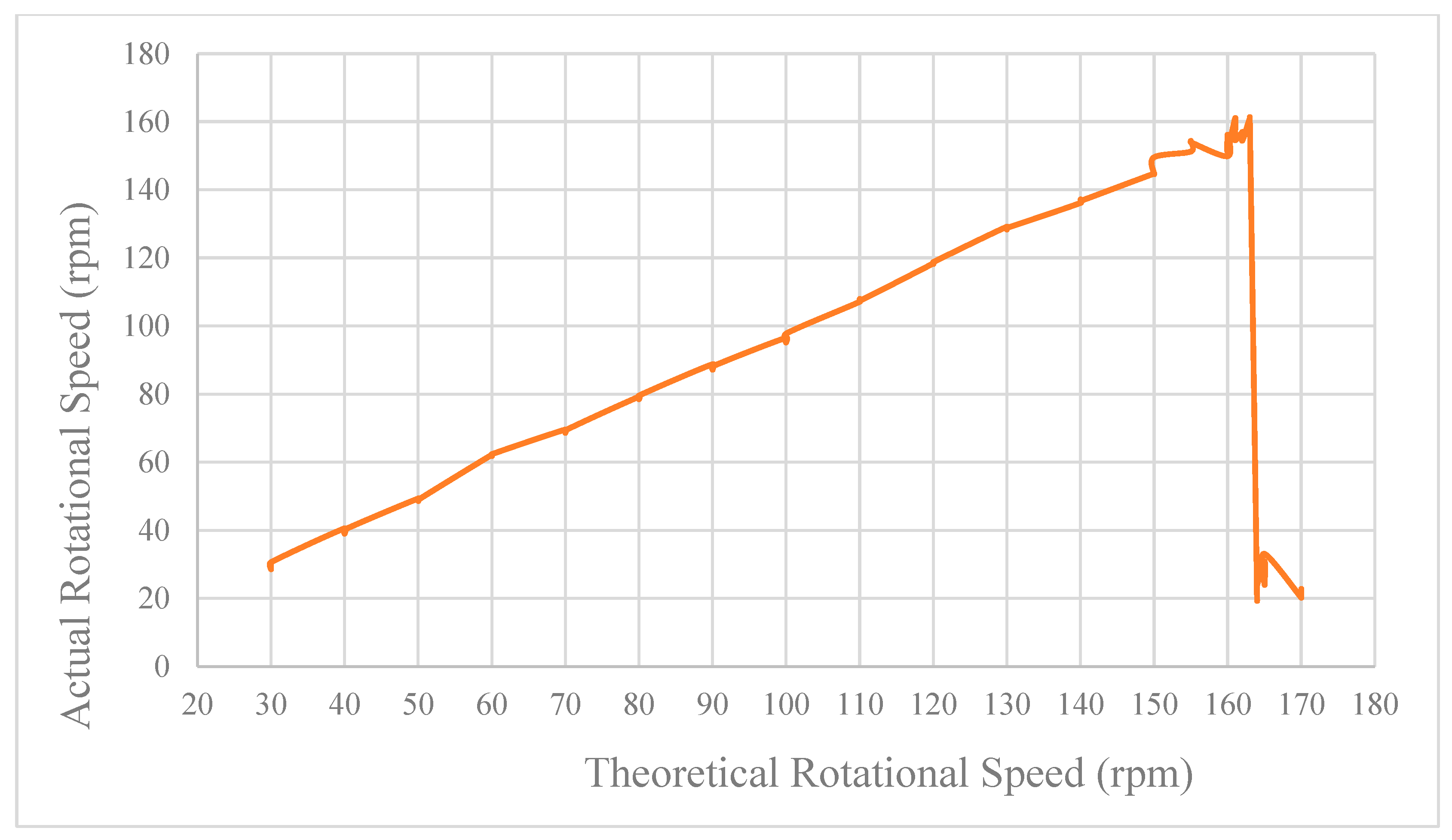
The calibration results revealed a strong linear correlation between the programmed and actual stepper motor speeds up to 164 rpm, beyond which deviations became more pronounced (Figure 7). This finding indicates reliable and predictable motor control within the 30–164 rpm range, which is critical for ensuring consistent feed output in automated systems. The findings also highlight the torque limitations of the NEMA 17 motor at higher speeds, where diminished output accuracy may impact dispensing precision. These results support the system’s operational suitability within the identified speed range, aligning with design objectives for accurate and efficient feed metering in aquaculture applications [14].

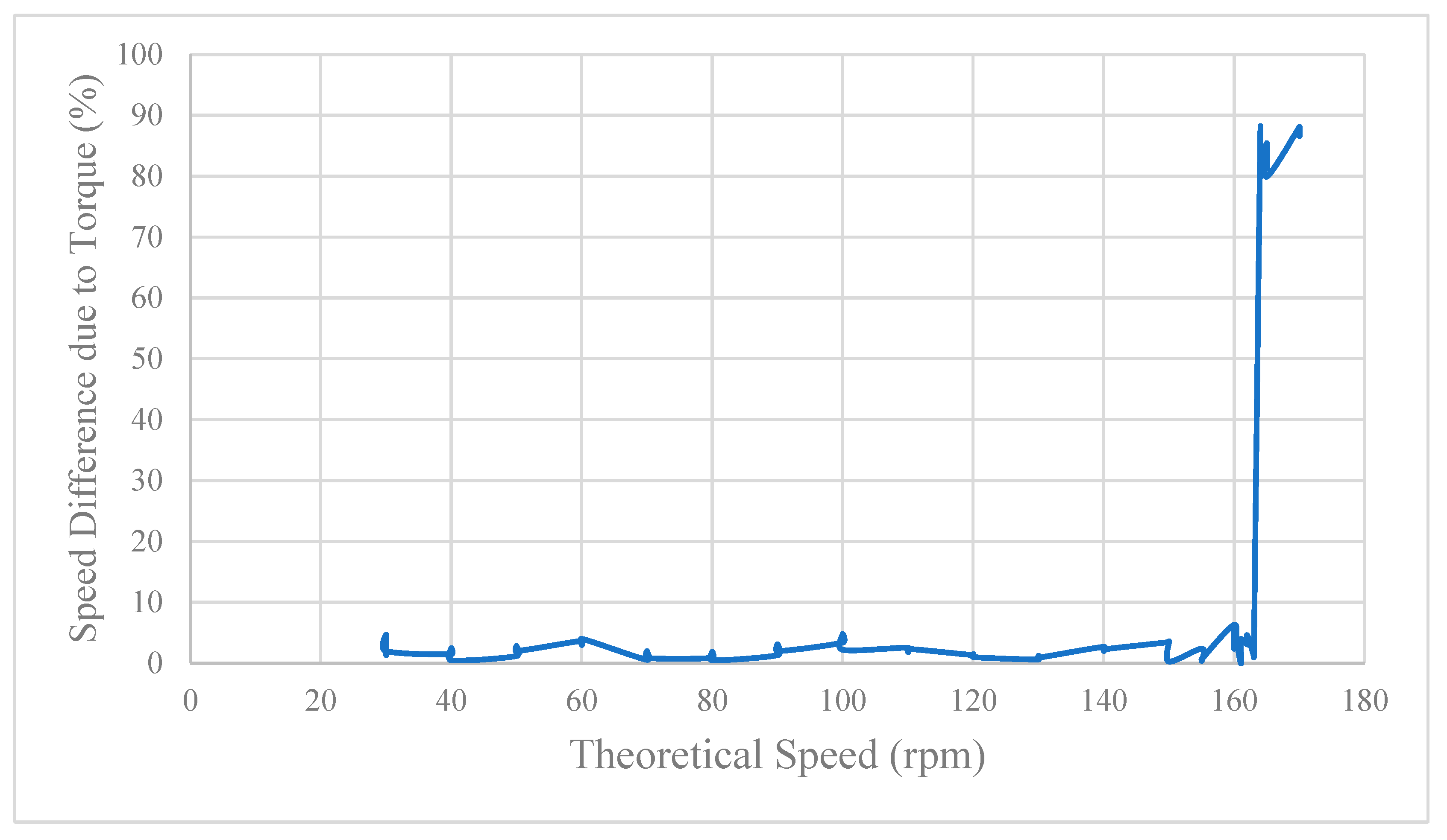
Beyond 164 rpm, the speed decreases sharply, indicating the system’s mechanical or electrical saturation point due to insufficient motor torque or increased friction [15]. Figure 8 shows that the percent speed deviation remained minimal up to 164 rpm but spiked to 82.22%, confirming control instability and torque transfer inefficiency.

The likely cause is the inherent torque drop-off of the NEMA 17 motor at high speeds and load resistance, resulting in skipped steps or stalled operations. Thus, 164 rpm represents the practical upper limit for reliable feed metering.

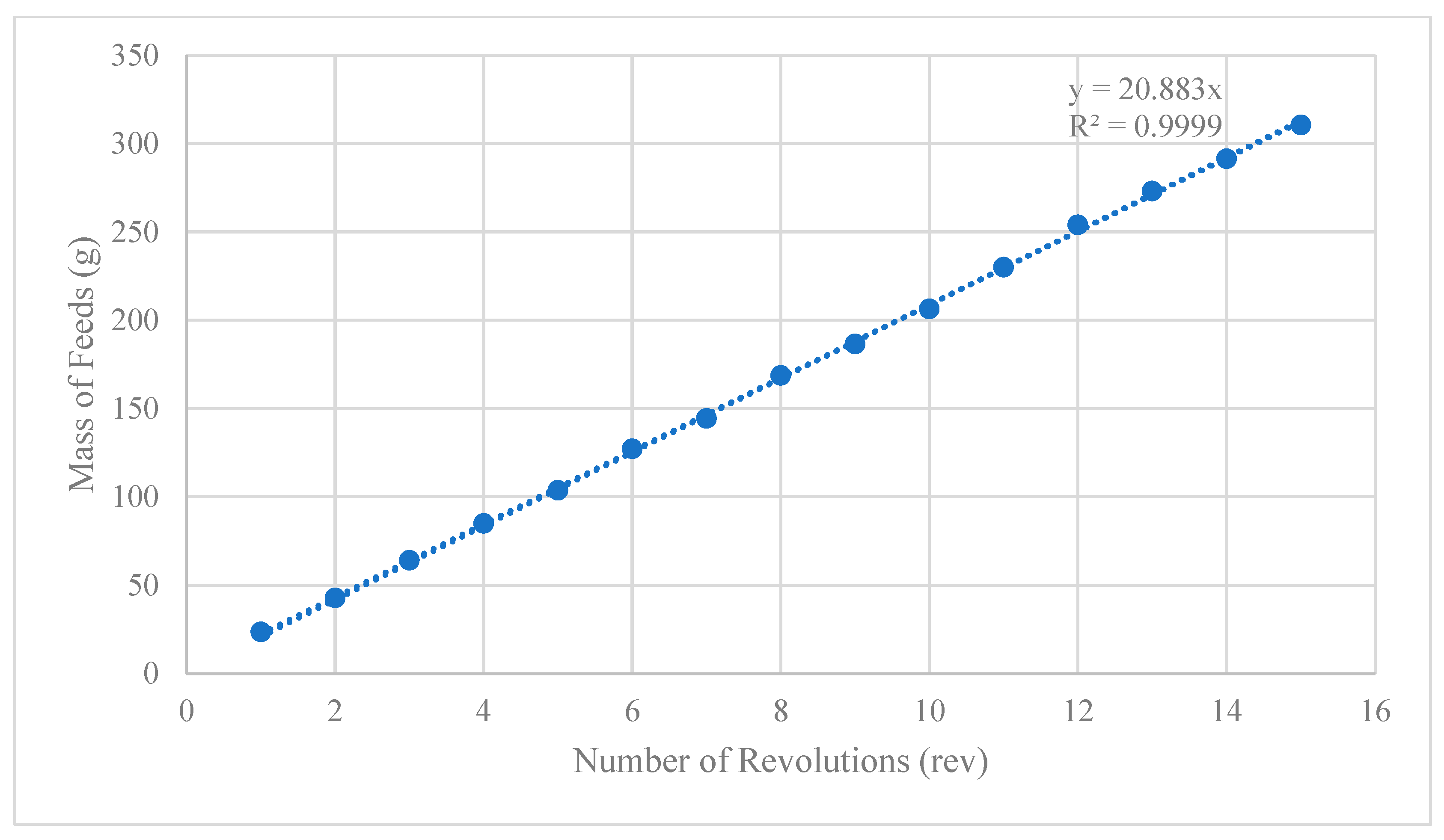
The calibration curve (Figure 9) yielded an R² value of 0.999, indicating a strong linear fit between auger revolutions and the feed mass delivered. This corresponds to a consistent feed rate of 20.883 g per revolution, enabling the control system to translate target feed masses into auger rotations accurately. At 163 rpm, the system delivered 100 g of feed in approximately 1.70 s, confirming its fast and precise dispensing capability with minimal error.

The established calibration curve is critical for ensuring precise and programmable feed delivery. The system eliminates assumptions by defining a fixed, linear relationship between auger revolutions and feed mass and enables consistent, repeatable feeding across multiple operations. This allows the automatic feeder to deliver accurate quantities based on user-defined input, supporting effective feed management, minimizing waste, and enhancing operational reliability in aquaculture applications.

3.2.2. Results of the Feed Dispersing Performance Test

Before modeling, Statistical analysis using a Box–Behnken design assessed the feeder’s performance across three input variables. Mean Radius Spread and High Concentration Area satisfied normality assumptions (p = 0.3425 and p = 0.8157, respectively), while Total Spread Area did not (p = 0.0142), indicating the need for alternative analytical approaches for that response in future studies (

Table 3. Test for normality using the Shapiro–Wilk test.

Parameter	p-Value	Interpretation
Mean Radius Spread	0.3425	Normally Distributed
Total Spread Area	0.0142	Not Normally Distributed
High Concentration Area	0.8157	Normally Distributed

).

Table 4. Experimental results from a three-factor Box and Behnken Methodology Design.

Run	Impeller Speed (RPM)	Feed Mass (g)	Time of Spread (s)	Average Radius Spread (cm)
	X1	X2	X3	Y
1	−1	−1	0	33.45
2	−1	1	0	42.86
3	−1	0	−1	45.73
4	−1	0	1	30.81
5	1	−1	0	51.78
6	1	1	0	50.87
7	1	0	−1	49.50
8	1	0	1	47.97
9	0	−1	−1	45.12
10	0	−1	1	35.45
11	0	1	−1	36.45
12	0	1	1	30.38
13	0	0	0	33.89
14	0	0	0	32.11
15	0	0	0	31.25

presents the experimental results obtained from the three-factor BBD, where the Average Radius Spread (cm) served as the response variable. The table summarizes the observed values across 15 experimental runs, reflecting the combined effects of impeller speed ($X_1$), feed mass per cycle ($X_2$), and time of spread ($X_3$) on feed dispersion.

Table 4 summarizes the experimental results of the three-factor BBD, with average radius spread (Y) as the response variable. Results showed that both impeller speed ($X_1$) and feed mass per cycle ($X_2$) had significant effects on feed distribution, while spreading time ($X_3$) contributed moderately. Increasing impeller speed and feed mass improved dispersion up to optimal levels, beyond which turbulence reduced uniformity. These findings are consistent with previous studies reporting that vortex-type impellers generate higher flow pressure and improved mixing efficiency [16], and that centrifugal impeller systems can achieve effective feed dispersion under controlled propulsion conditions [17]. Optimal operating conditions were achieved at moderate combinations of $X_1$ and $X_2$, resulting in consistent radial feed distribution under stable water flow and aeration. This result supports the system’s mechanical feasibility and its potential to deliver uniform, bottom-directed feed dispersion for shrimp aquaculture.

3.2.3. Regression and Analysis of Variance of the Experiment Results

An ordinary least squares (OLS) multiple linear regression model was used to assess the effects of rotational speed (rpm), mass, and time, including their quadratic and interaction terms, on the mean radius spread. The regression coefficients and associated analysis of variance (ANOVA) results are summarized in

Table 5. OLS regression model fit results for mean radius spread.

Metric	Value	Interpretation
R-Squared	0.919	Very Strong
Adj. R-Squared	0.773	Fairly Precise
F-Statistic	6.300	Good
Prob (F-statistics)	0.0283	Significant (p < 0.05)

. The model demonstrated a strong fit, with an R² value of 0.919, indicating that approximately 91.9% of the variability in the mean radius spread was explained by the predictors. The adjusted R² of 0.773 provides a more conservative evaluation of model performance by accounting for model complexity relative to the limited sample size (n = 15).

To formally assess model adequacy beyond goodness-of-fit statistics, a lack-of-fit test was conducted using replicated center points from the Box–Behnken design. The results of this analysis are presented in

Table 6. Lack-of-Fit Test Results.

Metric	Value *
Pure Error SS	3.6259
Pure Error DF	2
Lack-of-Fit SS	63.8361
Lack-of-Fit SS	3.0
F-statistics (Lack-of-Fit)	11.7372
p-value (Lack-of-Fit)	0.0795

* A p-value greater than the α = 0.05 is not significant.

. The lack-of-fit test yielded an F-statistic of 11.74 with a corresponding p-value of 0.0795, which exceeds the significance threshold of $\alpha =0.05$. This indicates that the lack of fit is not statistically significant, confirming that the quadratic regression model sufficiently represents the experimental response within the investigated design space.

The F statistic of 6.300 and a p value of 0.0283 confirm the model’s overall significance at the 5% level, indicating that at least one predictor meaningfully helps explain the response variable. The regression model offers quantitative insights into how rotational speed, mass, and time, along with their interactions, influence feed particle dispersion, as detailed in the coefficient estimates and p values presented in

Table 7. Ordinary Least Squares Regression Model Coefficient for Mean Radius Spread.

Predictor	Coefficient	p-Value *	Interpretation
Intercept	124.0996	0.004	Significant
Rotational Speed	−0.3322	0.011	Significant
Mass	−0.0623	0.591	Not Significant
Time	−7.1461	0.076	Borderline
Rotational Speed2	0.0004	0.005	Significant
Mass2	0.0003	0.238	Not Significant
Time2	0.1951	0.420	Not Significant
Rotational Speed~Mass	−0.0002	0.277	Not Significant
Rotational Speed~Time	0.0074	0.141	Not Significant
Mass~Time	0.0032	0.658	Not Significant

* A p-value less than the α = 0.05 is significant.

.

The multiple linear regression results revealed that the intercept (124.10, p = 0.004) was statistically significant, serving as a baseline for interpreting predictor effects, although it lacks practical meaning. Among the predictors, rotational speed was the only significant linear term (p = 0.011) with a negative coefficient (−0.3322), indicating that higher impeller speeds reduce the mean spread width. This reduction is attributed to vortex formation at elevated speeds, which pulls particles inward and limits radial dispersion, a finding that is consistent with previous fluid dynamics studies [18].

The quadratic term for rotational speed (p = 0.005, coefficient = 0.0004) suggests a U-shaped relationship where the spread radius decreases but increases again beyond a critical speed, reflecting the balance between centrifugal forces and vortex-induced inward drag. The feed mass had no significant effect on the spread width (p = 0.591), which aligns with research indicating that fluid flow dynamics, rather than mass alone, dominate dispersion behavior [19].

Time exhibited a negative but marginally nonsignificant effect (p = 0.074), suggesting that prolonged operation may reduce the spread width due to vortex development beneath the impeller, which is consistent with existing research on flow disruption in pumps [13,16]. All interaction terms (rotational speed × mass, rotational speed × time, and mass × time) were nonsignificant, suggesting that these variables act independently within the tested ranges. Overall, rotational speed emerged as the primary driver of feed spread behavior, emphasizing the need to calibrate optimal speed settings to balance dispersion and vortex control.

$$Y={\mathsf{\beta }}_0+{\mathsf{\beta }}_1{X}_1+{\mathsf{\beta }}_2{X}_2+{\mathsf{\beta }}_3{X}_3+{\mathsf{\beta }}_{11}{X}_1^2+{\mathsf{\beta }}_{22}{X}_2^2+{\mathsf{\beta }}_{33}{X}_3^2+{\mathsf{\beta }}_{12}{X}_1{X}_2+{\mathsf{\beta }}_{13}{X}_1{X}_3+{\mathsf{\beta }}_{23}{X}_2{X}_3$$

(1)

where:

• Y—is the predicted response of the mean radius spread;
• β₀—is the intercept of the model;
• X₁—is the rotational speed of the impeller (rpm);
• X₂—is the mass of the feed (g);
• X₃—is the time of spread (s);
• β₁—is the coefficient of the revolutions per minute of the impeller;
• β₂—is the coefficient of mass of the feed;
• β₃—is the coefficient of the time of spread.

$$Max Radius Spread=124.0996-0.3322RPM+0.0004{RPM}^2$$

(2)

The regression model demonstrates a statistically significant nonlinear (quadratic) relationship between impeller rotational speed (rpm) and the radial spread of feed particles. Specifically, the negative linear coefficient (β₁ = −0.3322) indicates that, at lower to moderate rpm levels, an increase in rotational speed results in a reduction in mean spread radius. In contrast, the positive quadratic coefficient (β₁₁ = 0.0004) reflects a reversal in this trend beyond a critical rotational speed threshold, where further increases in rpm are associated with an expansion of the radial spread. This results in a concave upward response surface, characteristic of a parabolic turning point.

These findings are consistent with established fluid dynamics principles. At moderate rotational speeds, impeller-induced vortical structures may develop, generating inward forces that diminish outward dispersion efficiency. As the rotational speed surpasses this critical threshold, the kinetic energy imparted to the fluid becomes sufficient to counteract these centripetal effects, thereby enhancing the radial dispersion of feed particles. Nonetheless, excessively high rotational speeds are likely to promote turbulence and energy dissipation, which are not fully accounted for within the constraints of the second-order polynomial model. This limitation suggests the need for complementary computational fluid dynamics (CFD) analyses to capture the system’s complex flow behaviors comprehensively.

The model’s intercept term (β₀ = 124.0996) serves as a statistical baseline, representing the predicted mean spread radius when all predictors are set to zero. However, this condition lacks practical relevance, as zero rotational speed, mass, and time inherently imply the absence of feed dispersion. While feed mass and spread time exhibited lower magnitude and statistically non-significant effects within the tested parameter ranges, their inclusion in the model provides additional capacity to detect higher-order or interaction effects that may arise under varying operational conditions. Collectively, the results confirm impeller rotational speed as the primary determinant of feed dispersion performance, with the quadratic model effectively capturing the system’s nonlinear and non-monotonic response patterns, which would otherwise remain undetected in a purely linear modeling framework.

3.2.4. Surface Response

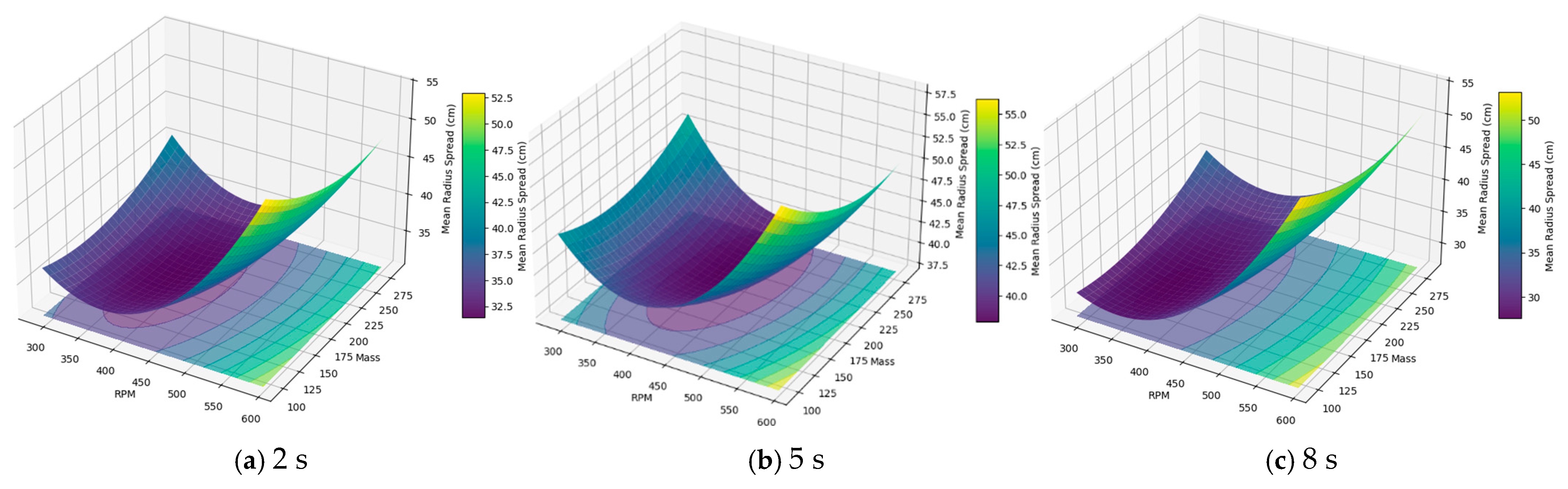
Three surface response plots were generated using the Box–Behnken experimental design data to better understand how the input variables influenced feed dispersion. All statistical analyses were conducted in Jupyter Notebook (Python 3.11) using the pandas, numpy, matplotlib, statsmodels, and scipy libraries. A second-order polynomial model was fitted using the ordinary least squares (OLS) method implemented in the statsmodels package, while model assumptions such as normality and homogeneity of variance were verified using the Shapiro and Levene tests, respectively. The resulting three-dimensional surface plots were visualized with matplotlib. The interactions between rotational speed, 285.98 rpm (low), 440.74 rpm (mid), and 586.85 rpm (high), and feed mass, 95.23 g, 190.45 g, and 285.68 g, were examined relative to the mean radius spread of feed, with each plot constructed at fixed spread durations of 2, 5, and 8 s. Across all conditions, rotational speed exerted the most significant influence on feed dispersion, as illustrated in Figure 10.

At 2 s (Figure 10a), maximum spread exceeds 55 cm, achieved at low-to-mid rpm and moderate feed mass, indicating efficient dispersion before fluid instabilities develop. High rpm settings already show a slight performance reduction, suggesting early vortex formation, which restricts outward feed movement. The surface reveals a broad, concave optimal zone centered at mid-range rpm, where centrifugal forces efficiently distribute the feed.

By 5 s (Figure 10b), the maximum spread slightly declines to ~52.5 cm, with noticeable performance drops at high rpm across all feed masses. The optimal operating zone narrows and shifts toward lower rpm, implying that vortex formation intensifies with time, undermining dispersion at higher speeds. This reflects the model’s quadratic findings, confirming that dispersion efficiency declines beyond a certain rpm threshold.

At 8 s (Figure 10c), dispersion patterns become more restricted, with optimal spread (~55 cm) confined to low rpm and feed mass. Both high rpm and feed mass significantly reduce spread, highlighting the progressive formation of stable vortex structures. These vortices draw particles inward, counteracting centrifugal dispersion and limiting feed coverage in the tank’s outer regions.

The overall trend shows that while moderate rpm and feed mass maximize early dispersion, prolonged operation requires progressively lower rpm settings to maintain effectiveness. Operating at excessive speeds over time enhances vortex-induced inward flow, reducing feed spread efficiency.

These results emphasize the need for dynamic rotational speed adjustment based on operating time to optimize feed dispersion and minimize waste in aquaculture systems. Maintaining the system within an efficient, vortex-minimized flow regime is essential for consistent feed coverage.

3.2.5. Cross-Validation of the Response Surface Model

Leave-one-out cross-validation (LOOCV) was conducted as an internal robustness check for the quadratic response surface model due to the limited number of experimental runs inherent to the Box–Behnken design. LOOCV is commonly applied to small-scale, structured experimental datasets to assess model stability and generalizability when independent validation experiments are not feasible [20]. In the context of response surface methodology, LOOCV has been shown to be particularly useful for evaluating local predictive behavior within the design space rather than for establishing global predictive performance [21]. 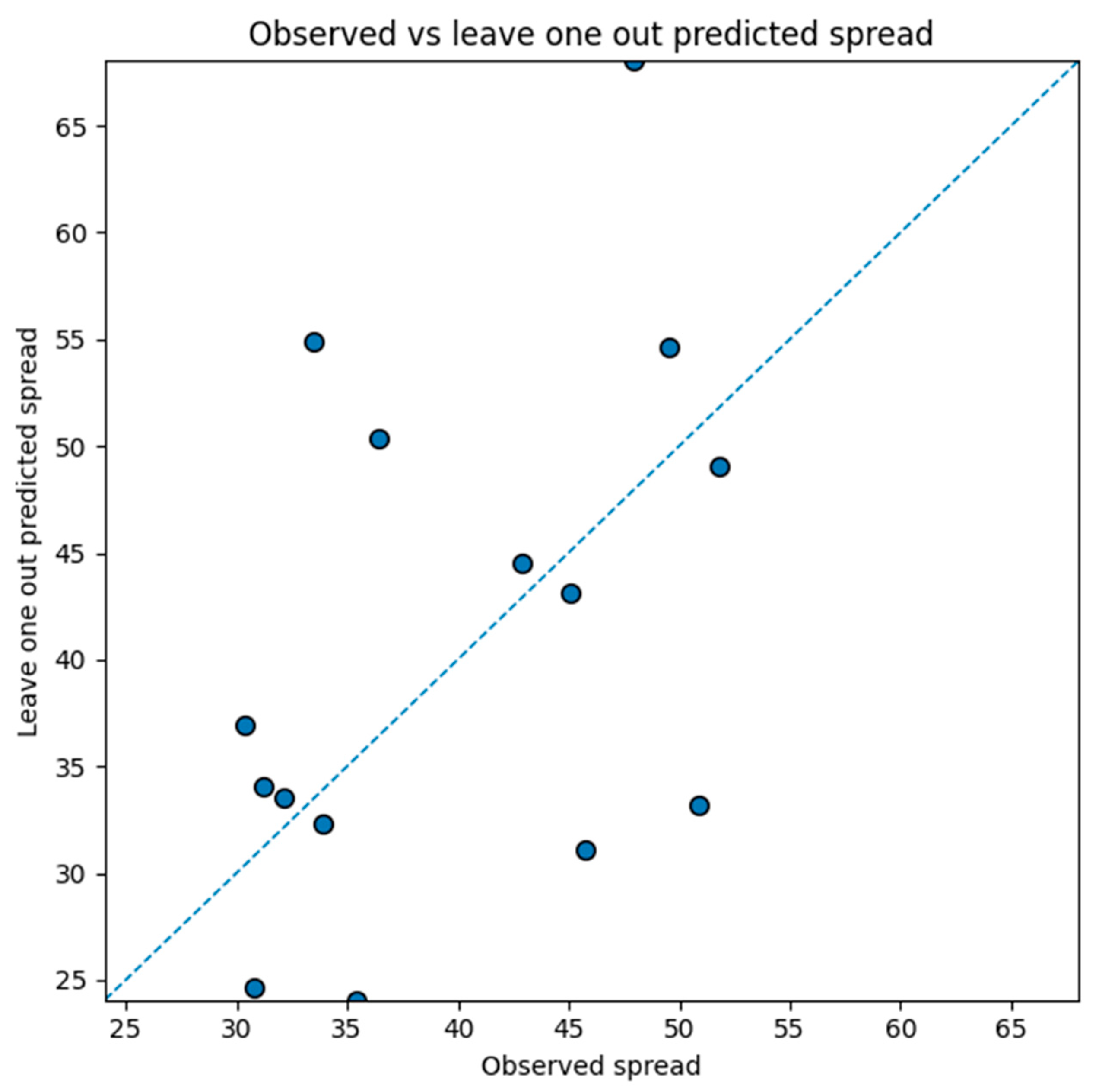Figure 11 illustrates the relationship between observed mean radius spread values and LOOCV-predicted responses. The dashed line represents the line of equality (y = x), where predicted values perfectly match observed values; points lying closer to this line indicate higher predictive accuracy. Predictions show closer agreement near the center of the design space, while larger deviations occur at boundary points, consistent with the expected behavior of response surface models derived from Box–Behnken designs.

The LOOCV analysis yielded a predicted $R^2$ of −1.03, compared with an adjusted $R^2$ of 0.665 for the fitted model, indicating limited predictive accuracy for individual unseen runs. A negative predicted $R^2$ implies that, when predicting unseen observations, the model performs worse than simply using the overall mean response. This outcome does not indicate that the response surface model is ineffective; rather, it reflects weak predictive robustness for individual runs, which is commonly observed in Box–Behnken designs with very limited experimental runs. Importantly, although optimization results are often visualized or discussed in terms of a single factor (e.g., impeller rotational speed), the fitted response surface is inherently multivariate, as it was developed from simultaneous variations in rotational speed, feed mass, and dispersion time. Consequently, the response cannot be fully expressed or predicted as a univariate function of rotational speed alone without specifying the remaining parameters. Analysis of the prediction residual sum of squares (PRESS = 1843.69) further revealed that approximately 86% of the total prediction error originated from a small number of runs located at the boundaries of the experimental domain, while runs near the center exhibited relatively small errors. This behavior highlights the local and multivariate nature of quadratic response surface models, which provide the most reliable predictions within regions of high data density and increased uncertainty at extreme combinations of the design variables.

Characterization analysis of the quadratic response surface model was conducted to describe the nonlinear relationship between impeller rotational speed and feed dispersion behavior within the Box–Behnken design space, with model reliability first assessed through LOOCV. As shown in Figure 11, predictive agreement is strongest near the center of the experimental domain, where data density is highest, while increased deviations occur at boundary conditions. Within this validated context, analysis of the fitted model identified an operating point at approximately 415 rpm, corresponding to a predicted mean radius spread of 31.59 cm. This speed was selected because it lies near the central region of the response surface, where the Box–Behnken design provides balanced factor variation and reduced estimation variance compared with boundary points. To account for model uncertainty, the estimated response was accompanied by a 95% confidence interval (26.16–37.02 cm) and a 95% prediction interval (20.70–42.49 cm), representing uncertainty in the estimated mean and the expected variability of individual experimental outcomes, respectively. The results indicate that feed dispersion improves with increasing rotational speed up to a threshold, beyond which further increases in speed or prolonged dispersion duration promote the formation of a strong central vortex. This vortex induces localized recirculation and vertical flow dominance, which negatively affects radial feed transport and reduces dispersion uniformity. Accordingly, the identified operating point should be interpreted as an efficient condition within the central region of the investigated experimental domain, where hydrodynamic behavior remains stable and model predictions are most reliable, rather than a globally optimal setting applicable beyond the tested parameter space.

3.2.6. Coefficient of Variation (CV) from Image-Based Spread Analysis

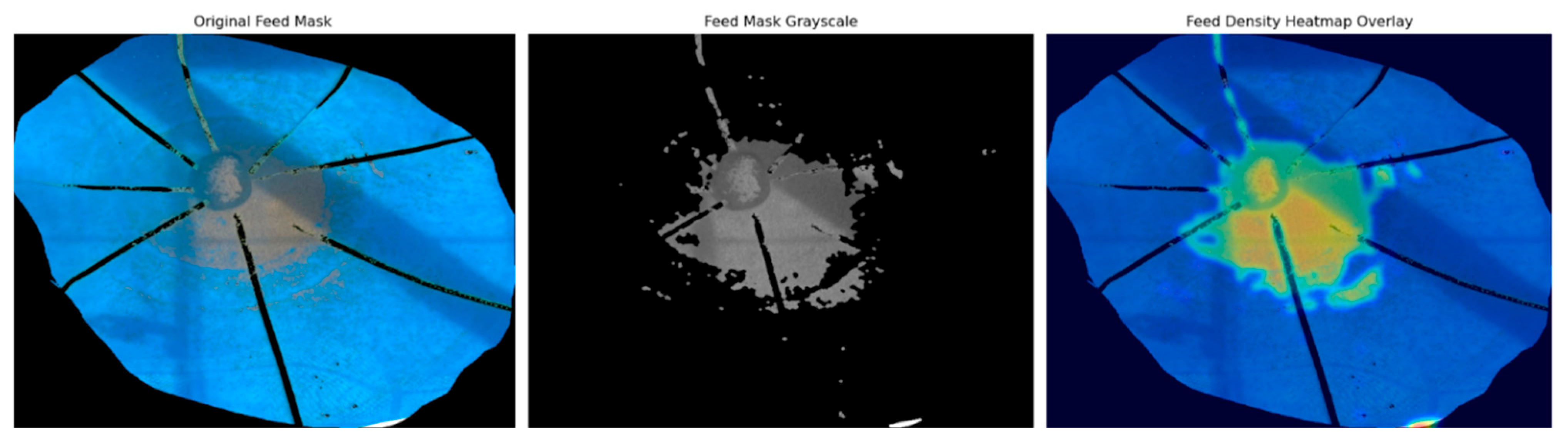
Image analysis via OpenCV in Python was applied to evaluate feed dispersion consistency through the coefficient of variation (CV), which quantifies spatial variability by comparing high-concentration feed zones to the total dispersed area. The visual outputs included binary masks, grayscale intensity plots, and heatmaps, offering insight into dispersion patterns (Figure 12).

The results revealed a central feed concentration with a limited radial reach, which was likely due to the impeller geometry and insufficient outward velocity. At higher RPMs, vortex formation and centripetal flow may trap feed centrally, whereas physical feed properties, such as pellet density and moisture content, further limit dispersion due to rapid settling. The feed density heatmap overlay in Figure 12 shows this distribution pattern, where warmer colors (yellow to red) indicate higher feed concentration and cooler colors (blue to green) represent lower feed density across the tank surface. These findings are consistent with the surface response results, indicating a reduced mean spread at high speeds.

The lowest CV (0.13) occurred in Run 4 (low RPM, middle mass, high time), suggesting that a longer dispersion time and lower impeller speed promote stable flow fields and more uniform feed spread. High-speed trials (CV = 0.21–0.25) resulted in a localized but consistent distribution, whereas mid-speed, low-mass/time runs (CV = 0.32–0.35) presented greater variability, highlighting the sensitivity of feed spread to interaction effects.

4. Conclusions and Future Work

An automatic aquaculture bottom feeder prototype was successfully designed, fabricated, and evaluated as a functional electromechanical system for precise feed delivery in tank-based shrimp aquaculture. The system incorporated a 3D-printed auger for accurate feed metering and a closed-type centrifugal impeller for radial feed dispersion, both controlled via an Arduino Uno microcontroller. The use of 3D modeling and additive manufacturing enabled a compact, modular, and customizable structure suitable for rapid prototyping and mechanical optimization. Experimental evaluation using the Box–Behnken response surface methodology (BBD–RSM) identified impeller rotational speed as the only statistically significant factor affecting feed dispersion (p = 0.010), while feed mass, dispersion time, and interaction effects were not significant. Image-based analysis using OpenCV quantified feed uniformity through the coefficient of variation (CV), revealing that the most uniform distribution (CV = 0.13) occurred at lower impeller speeds and longer dispersion durations.

The findings highlight a gap in existing aquaculture standards [10], which lack specific provisions for water-surface or near-bottom feed dispersion mechanisms designed for benthic species. The developed prototype offers a novel, programmable, and energy-efficient feeding solution capable of delivering sinking pellets uniformly to the tank bottom, thereby improving feeding accuracy and minimizing waste.

Future work should focus on extending the present characterization-oriented analysis through targeted sensitivity studies to further quantify the relative influence of operational parameters and assess system robustness. Economic evaluation is also required to determine production scalability, manufacturing feasibility, and cost-effectiveness for commercial deployment. In addition, biological validation under actual culture conditions remains essential and should include assessments of shrimp feeding behavior, growth performance, feed conversion efficiency, and potential physical injury or stress associated with mechanical feed dispersion, particularly at higher impeller speeds or prolonged operation. Further investigations should examine the effects of feed pellet size and density on dispersion performance, as well as refinements to impeller geometry, outlet angle, and immersion depth. The integration of real-time feedback control and environmental sensing is also recommended to enhance precision, adaptability, and long-term sustainability in intensive aquaculture systems.