
Article

UAV-Borne RGB Imagery and Machine Learning for Estimating Soil Properties and Crop Physiological Traits in Peanut (Arachis hypogaea): A Low-Cost Precision Agriculture Approach

by
Wilson Saltos-Alcivar
1,
Cristhian Delgado-Marcillo
2,
Ezequiel Zamora-Ledezma
3,*,
Carlos A. Rivas
4 and
Henry Antonio Pacheco Gil
2,*
1
Facultad de Posgrado, Universidad Técnica de Manabí, Portoviejo 130150, Ecuador
2
Departamento de Ciencias Agrícolas, Facultad de Ingeniería Agrícola, Universidad Técnica de Manabí, Lodana 13132, Ecuador
3
Laboratorio de Funcionamiento de Agroecosistemas y Cambio Climático FAGROCLIM, Departamento de Ciencias Agrícolas, Facultad de Ingeniería Agrícola, Universidad Técnica de Manabí, Lodana 13132, Ecuador
4
Mediterranean Forest Global Change Observatory, Digitalization and Development in Forestry Ecosystems Laboratory, Department of Forestry Engineering, DigiFoR+-ERSAF, University of Cordoba, Campus de Rabanales, Crta. IV Km. 396, 14071 Córdoba, Spain
*
Authors to whom correspondence should be addressed.
AgriEngineering 2026, 8(5), 177; https://doi.org/10.3390/agriengineering8050177
Submission received: 15 February 2026 / Revised: 19 April 2026 / Accepted: 22 April 2026 / Published: 2 May 2026
(This article belongs to the Topic Digital Agriculture, Smart Farming and Crop Monitoring)

Abstract

Modern agriculture must balance productivity with sustainability. In this context, unmanned aerial vehicles (UAVs) offer flexible, cost-effective tools for crop and soil monitoring in precision agriculture. This study aimed to evaluate the potential of UAV-borne RGB imagery, combined with vegetation indices and machine learning, to estimate surface soil properties and crop physiological traits in peanut (Arachis hypogaea) cultivation. A factorial field experiment with four varieties, two planting densities, and two tillage systems was monitored using high-resolution RGB orthomosaics acquired at key phenological stages. From these images, 17 RGB-based indices were computed and related to soil variables and crop traits using Spearman correlation and two regression algorithms: Random Forest (RF) and k-Nearest Neighbors (KNN). RF models outperformed KNN, with the Red Chromatic Coordinate (RCC) index achieving an R2 of 0.87 for predicting soil organic matter content. Indices such as visible NDVI and the Green Vegetation Index also provided robust estimates of canopy condition and leaf chlorophyll. Overall, the results demonstrate that UAV RGB imagery, processed through simple vegetation indices and RF models, constitutes an effective, low-cost approach for monitoring key agronomic parameters in peanut farming.

1. Introduction

Rapid global urbanization poses a major challenge to agri-food systems. In 2018, 55% of the world’s population lived in urban areas, and this proportion is projected to rise to 68% by 2050 [1,2]. Such demographic and spatial expansion drives increasing food demand, which is expected to grow by 35–56% by the middle of this century [1]. At the same time, climate variability and growing pressure on both green and blue water resources are pushing agricultural systems to the limits of sustainability. This situation demands maximizing resource productivity through sustainable methods and practices that ensure food production without degrading the environment [3]. Furthermore, biodiversity loss and ecosystem degradation—mainly driven by land-use change and agricultural intensification—represent serious threats to human well-being, underscoring the urgent need for integrated approaches that balance production and conservation objectives [2].
The use of unmanned aerial vehicles (UAVs, or drones) as remote sensing platforms has attracted increasing attention in precision agriculture due to their operational flexibility and capacity to generate high spatial and temporal resolution imagery of agricultural fields [4]. UAV-based data acquisition is emerging as an effective alternative for crop management, monitoring, and regulation across different growth stages, with the goal of enhancing productivity and reducing operational costs [5]. In agricultural applications, UAVs equipped with infrared and RGB cameras allow detection of crop health anomalies by identifying color variations associated with disease onset [6].
Within this context, precision agriculture (PA) regards remote sensing as a key analytical tool. By combining multispectral imagery with vegetation index analyses, drones can accurately assess crop conditions, enabling timely agronomic adjustments [7]. This technology thus helps improve soil health, preserve water quality, and foster local economic growth—promoting a more efficient and sustainable farming system [8].
In recent years, the integration of remote sensing and machine learning has emerged as a powerful framework for quantifying crop and soil variability in precision agriculture. One critical dimension of this framework is the use of multi-temporal spectral features as predictors: vegetation indices and spectral bands extracted at multiple phenological stages capture the dynamic trajectory of canopy development and surface soil conditions, substantially improving model predictive power compared to single-date observations. For example, Camenzind and Yu (2023) demonstrated that multi-temporal multispectral UAV imagery, analyzed with Random Forest models, enabled wheat yield prediction before flowering, with performance varying markedly depending on the phenological stage at which indices were computed [9]. Similarly, Giannico et al. (2024) showed that Random Forest trained on time-series Sentinel-2 vegetation indices could estimate vine stem water potential with R2 = 0.72 in testing, outperforming linear regularization approaches (lasso, ridge, elastic net), and they applied the resulting model to generate spatiotemporal prediction maps of vineyard water status under semi-arid conditions [10]. A key methodological strength of ensemble learners such as Random Forest in this context is their ability to model complex, nonlinear relationships between spectral signals and biophysical variables, and to remain robust under the strong inter-index collinearity that is inherent to spectral datasets derived from overlapping RGB or multispectral bands [10,11]. Unlike linear models, Random Forest does not require the input predictors to be orthogonal or normally distributed, and its bagging strategy reduces variance without requiring explicit collinearity correction [11]. Nevertheless, a recognized limitation of site-specific or single-season ML models is their constrained transferability: models calibrated at a single location under particular climatic, soil, and management conditions tend to show degraded performance when applied to new sites or growing seasons due to differences in phenological timing, sensor configuration, and environmental gradients [10,12,13,14]. This combined use of remote sensing and machine learning therefore represents a key technological pillar for advancing operational crop monitoring and decision-making in precision agriculture, while simultaneously highlighting the need for multi-site, multi-season validation to strengthen the generalizability of the resulting predictive models.
Peanut (Arachis hypogaea L.) ranks as the sixth most widely cultivated oilseed crop globally and plays a significant role in nutritional security due to its high contents of fats, proteins, minerals, and vitamins [15]. In Ecuador, according to the 2025 Continuous Agricultural Area and Production Survey (ESPAC), peanut was cultivated on 2943.94 hectares, yielding 2748.47 metric tons [16]. Peanut productivity is influenced by multiple factors, notably agronomic design, land preparation, planting density, and fertilization strategies [17]. As a leguminous species, peanut has the capacity to fix atmospheric nitrogen and enrich the soil, thereby reducing dependence on nitrogen fertilizers [18,19].
Tillage systems represent a key agronomic factor influencing soil physical and chemical properties, and consequently crop performance. Conventional tillage (CT) involves mechanical soil disturbance that disrupts soil aggregates, accelerates organic matter decomposition, and may increase bulk density over time, while zero tillage (ZT) minimizes soil disturbance, preserving soil structure, moisture retention, and organic carbon content [20]. In peanut (Arachis hypogaea L.) cultivation specifically, tillage practices have been shown to significantly affect soil bulk density, porosity, and nutrient availability—properties directly linked to root development, nodulation efficiency, and pod yield [21]. These contrasting tillage systems therefore generate measurable differences in soil surface conditions that can potentially be captured through spectral indices derived from UAV-based RGB imagery, making tillage type a relevant factor to consider in remote sensing-based crop monitoring studies.
In agriculture more broadly, rapid, accurate, and cost-effective yield estimation is crucial due to its technical, economic, and statistical implications for minimizing losses [22]. Accordingly, crop monitoring based on vegetation indices derived from RGB imagery provides accessible tools and innovative approaches for precise phenological tracking and improved yield estimation [23,24]. For instance, a study on wild blueberry crops demonstrated the accuracy of machine learning models in predicting the yield from aerially derived visual features [25], while another highlighted the importance of vegetation indices for estimating aerial biomass in oat crops across different growth stages [26].
UAVs equipped with RGB cameras have also proven highly effective for sugarcane yield estimation, accurately mapping plant height and stem density. These data assist in planning agricultural operations such as harvesting and milling, optimizing production efficiency [27]. In the case of remote sensing applications to peanut cultivation, UAV-based studies have shown promising results in estimating seedling emergence rates, confirming the utility of this technology during early growth stages [28]. Similarly, satellite imaging studies focused on peanut area and yield estimation have achieved high precision, consolidating these methods as viable alternatives for large-scale agricultural monitoring [29].
Building on these precedents, the present study aimed to monitor key agronomic conditions of peanut (Arachis hypogaea) cultivation through UAV-based remote sensing using an RGB camera, with the overarching goal of improving the efficiency of agricultural resource use. The monitoring focused on assessing variables related to crop nutritional status and development, including surface soil properties, physiological indicators of photosynthetic activity, and yield-related parameters. By analyzing spectral indices derived from RGB imagery, this research sought to explore the predictive potential of UAV-based imaging for estimating these conditions at strategic phenological stages of the crop.

2. Materials and Methods

2.1. Study Area

The study was conducted on experimental fields belonging to the Lodana Campus of the Faculty of Agricultural Engineering (Universidad Técnica de Manabí), located in the Lodana parish, Santa Ana canton, Manabí Province, Ecuador. The site is geographically positioned at projected UTM (Universal Transverse Mercator) coordinates: Easting 568,396 m, Northing 9,869,977 m, Zone 17 South, with an average elevation of 70 m above sea level (Figure 1).

2.2. Experimental Design and Variables Evaluated

In this study, the spectral response of edaphic properties (EP), root traits (nodule weight, NW), and foliar traits (crop chlorophyll level, CL) were evaluated through the analysis of 17 RGB spectral indices (SI) (Table 1). These indices were selected based on the work of Biró et al. (2024), a comparative study that reported significant differences among the RGB indices analyzed and demonstrated their usefulness for characterizing crop conditions and their components [30].
Among these indices, the visible Normalized Difference Vegetation Index (vNDVI) deserves particular attention. vNDVI is a vegetation index computed exclusively from the visible bands (red, green, and blue), which allows NDVI-like information to be derived from conventional RGB imagery acquired with low-cost digital cameras mounted on UAVs. Unlike the standard NDVI, which requires both red and near-infrared (NIR) bands and is therefore restricted to multispectral or satellite sensors, vNDVI was specifically designed to estimate NDVI values from RGB data using a genetic-algorithm-based formulation and has been shown to reproduce NDVI with high accuracy (overall mean percentage error ≈ 7%). For this reason, vNDVI was included in our analysis as a cost-effective proxy for NDVI under the RGB-only sensor configuration used in this study.
The experimental design followed a 4 × 2×2 factorial arrangement (Factor A × Factor B × Factor C) with three replications, yielding 16 treatment combinations (Table A1, Appendix A). Each experimental plot measured 3 m × 20 m (60 m2), for a total study area of approximately 1 ha. Factor A comprised four peanut varieties released by the Instituto Nacional de Investigaciones Agropecuarias (INIAP): INIAP-381 Rosita, INIAP-383 Pintado, INIAP-380 Charapoto, and INIAP-382 Caramelo. They were selected for their agronomic relevance and adaptability to local growing conditions. Factor B included two planting densities, 62,500 plants ha−1 (0.2 m × 0.8 m spacing, the density recommended by INIAP) and 100,000 plants ha−1 (0.2 m × 0.5 m spacing), to assess the effect of intraspecific competition on crop development. Factor C evaluated two tillage systems: zero tillage (ZT), in which no mechanical soil disturbance was applied, and conventional tillage (CT), which consisted of a single primary tillage pass using a moldboard plow to a working depth of 15 cm, aimed at breaking up the topsoil layer and incorporating surface residues prior to sowing (Table A1, Appendix A).
A total of eleven edaphic characteristics were analyzed, as described below. Soil samples were collected at 0–20 cm depth from three representative points per experimental plot using a stratified random sampling approach. The sub-samples were then thoroughly homogenized to form one composite soil sample per plot. For physical properties requiring undisturbed structure (bulk density, porosity, and Gravimetric Water Content), samples were collected using stainless steel volumetric cylinders (100 cm3) driven manually into the soil profile with a rubber mallet to minimize compaction artifacts. For chemical analyses (pH, Electrical Conductivity, organic matter, total nitrogen, phosphorus, and potassium), disturbed composite samples were collected by mixing the three sub-samples per plot, air-dried, sieved through a 2 mm mesh, and stored in labeled polyethylene bags prior to laboratory analysis. All soil sampling was conducted during the first UAV flight mission, coinciding with the early vegetative stage (0–15 days after sowing), to characterize baseline edaphic conditions before significant crop development.
Among the physical properties, soil porosity (%), representing the proportion of pore space relative to total sample volume, was calculated from particle density (γ) and soil bulk density (SBD) using Equation (1):
Porosity   % = γ S B D γ × 100
Soil bulk density, SBD (g·cm−3), defined as the dry mass of soil solids per unit total volume, was determined using the volumetric cylinder method, according to Equation (2) [31,32]:
S B D = m d s V
Particle density (γ, g·cm−3) was determined using the pycnometer method on pulverized, oven-dried soil samples immersed in distilled water, following Equation (3) [28,33]:
γ = W 2 W 1 W 4 W 1 ( W 3 W 2 )   γ w        
where W1 = pycnometer weight (g); W2 = pycnometer + 20 g soil (g); W3 = pycnometer + soil + distilled water to 100 mL (g); W4 = pycnometer + distilled water to 100 mL (g); and γ_w = 1 g·cm−3 [33].
Field capacity moisture content (θ_FC, %) was estimated using the Peele model (Equation (4)), and the permanent wilting point (θ_PWP, %) was calculated using the Briggs model (Equation (5)), both as functions of sand (SP), silt (SiP), and clay (CP) percentages and SBD [32]:
θ F C = 0.48 C P + 0.162 S i P + 0.023 S P + 256 S B D  
θ P W P = 0.302 C P + 0.102 S i P + 0.0147 S P S B D
Soil texture (% sand, silt, and clay, fraction < 2 mm) was determined by the Bouyoucos hydrometer method based on Stokes’ law of sedimentation, using Equations (6)–(8) [34]:
s a n d P = 100 S i P c 1 M s 100
c l a y P = S i P c 1 M s 100
s i l t P = 100 s a n d P + c l a y P
where SiPc1 = hydrometer reading corrected at 40 s (g·L−1); SiPc2 = hydrometer reading corrected at 2 h (g·L−1); and Ms = dry soil mass [34].
Among the chemical properties, Electrical Conductivity (EC, dS·m−1) was measured in a 1:2 or 1:5 soil–water suspension using a portable multiparameter device [34]. Soil pH was determined in a 1:2.5 soil–water suspension with a combined glass electrode under standardized conditions [34]. Total nitrogen (N, mg·kg−1) was quantified by the persulfate digestion method with spectrophotometric determination at 220–275 nm [35]. Potassium (K, mg·L−1) was determined by the tetraphenylborate gravimetric method [36], and phosphorus (P, mg·L−1) by acid persulfate digestion followed by colorimetric analysis using the molybdate–ascorbic acid method [30,31,36].
Soil organic matter (SOM, %) was quantified by the loss-on-ignition method at 600 °C, according to Equation (9):
S O M   % = m i m f m i 100                                              
where mi = oven-dried mass at 105 °C and mf = mass after calcination at 600 °C.
All physical and chemical soil parameters were subsequently correlated with UAV-derived spectral indices to assess their relationship with soil nutrient status, biomass development, and peanut crop yield potential within the study area.

2.3. UAV Flight Design and Phenological Synchronization for Data Acquisition

To fulfill the research objectives, two UAV flight missions were conducted in synchronization with in situ agronomic measurements at specific phenological stages of the peanut (Arachis hypogaea) crop. The first mission was carried out during the early vegetative stage (0–15 days after sowing) [37], coinciding with the collection of soil samples. The second mission was executed during the maturation and harvesting stage (80–120 days) [37], concurrently with chlorophyll content measurements and root nodule assessments. This strategic scheduling ensured that both the spectral and field-collected data were representative of consistent phenological and environmental conditions at each evaluated time point.
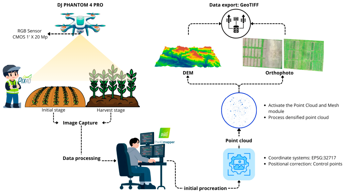
To execute the UAV-based surveys, a DJI Phantom 4 Pro platform equipped with an RGB camera featuring a 1-inch CMOS sensor (20 Mpx effective resolution) was employed. The flight plan was designed using Pix4Dcapture mobile application (Pix4D SA, Prilly, Switzerland). A georeferenced rectangular polygon encompassing the entirety of the study area was delineated, and the flight parameters were configured following the recommendations established by Anfruns Espuña (2023) [38] (Table 2).
The captured images were processed through a photogrammetric workflow using Pix4Dmapper software (v4.10.1, Pix4D SA, Lausanne, Switzerland), which is widely recognized for its autonomy and computational efficiency. This procedure enabled the generation of georeferenced orthomosaics of the study area from the visible bands (RGB) acquired during each flight mission. To ensure the spatial accuracy of the resulting orthomosaics, six ground control points (GCPs) were surveyed using a high-precision GNSS RTK Topcon GR-5 receiver. The coordinates of these control points were obtained using a static surveying method, which provided high positional accuracy and minimized geometric errors during image processing. This procedure ensured an adequate spatial correction of the orthomosaics; the workflow adopted for the analysis is summarized in Figure 2.
Based on the orthomosaics generated through the photogrammetric analysis, vegetation indices (VIs) were calculated using QGIS version 3.44.x “Solothurn”. The RGB bands of the orthomosaics obtained in each flight session were integrated and processed with the “Raster Calculator” tool, where the corresponding equations were applied to derive the values of each vegetation index (Table 1).

2.4. Statistical Analysis and Data Processing

Statistical analyses were performed using Python v3.10 and the Anaconda distribution (Anaconda Inc., Austin, TX, USA), with the following libraries: NumPy v1.24, pandas v1.5, SciPy v1.10, and scikit-learn v1.2. A spatial analysis of variance was conducted to evaluate treatment variability as a function of their spatial distribution, identifying potential significant differences among replications within the study area.
Additionally, data normality was assessed using the Shapiro–Wilk test [39]. Since the results indicated that the data did not follow a normal distribution, a Spearman rank correlation analysis was applied between soil variables, crop traits, and spectral indices. This analysis aimed to explore the relationships among these variables and to evaluate their potential as indicators of soil and crop properties. The classification of correlation strength was performed according to the criteria summarized in Table 3. Details on the statistical analyses and the criteria applied are provided in Appendix A (Table A2, Table A3 and Table A4).
To complement the classical statistical analysis and to develop robust predictive models for the estimation of agronomic variables, machine learning algorithms from the Scikit-learn library in Python were implemented. Two algorithms with different theoretical foundations were selected: k-Nearest Neighbors (KNN), an instance-based method, and Random Forest (RF), an ensemble method based on decision trees.
The k-Nearest Neighbors (KNN) algorithm relies on the principle that similar samples occur in close proximity within the feature space. To predict the value of a new observation, the algorithm identifies the k observations in the training set that are most similar to it based on a distance metric, commonly the Euclidean distance between two points p and q in an n-dimensional space, expressed by Equation (10) [42]:
    d ( p , q ) =   i = 1 n   q i p i 2                
where d ( p , q ) represents the Euclidean distance calculated between two points p and q in the multi-dimensional feature space. In this context, p and q are vectors corresponding to two individual observations, and each component of the vectors ( p i and q i ) is the specific value of a given feature or predictor variable for that observation. The subscript i iterates over the n features that define the space, so the formula computes the square root of the sum of squared differences across all features, providing a direct geometric measure of similarity between observations. A smaller distance indicates that the points are closer and therefore more similar in terms of their spectral signature, which is the fundamental principle exploited by the k-Nearest Neighbors (KNN) algorithm to perform clustering or prediction tasks [42,43].
For regression, the final prediction is obtained as the average of the target variable values of these k neighbors. The optimal choice of the hyperparameter k and the scaling of the features are critical for model performance, which has been validated in crop classification tasks using multispectral imagery [42].
In contrast, Random Forest (RF) is an ensemble algorithm that constructs a large number ( N ) of decision trees during training. Each tree is trained on a bootstrap sample of the original dataset and considers a random subset of features at each split, which reduces variance and overfitting. For regression, the forest aggregates the predictions of all individual trees by computing their average, as expressed in Equation (11) [43,44]:
                    y ^ = 1 N i = 1 n y i ^            
where y ^ i is the prediction of the i -th tree. This approach not only provides high predictive accuracy but also allows quantifying the importance of predictor variables (spectral indices), indicating which ones contribute most to the estimation of parameters such as chlorophyll content or nodule weight, which is particularly useful for plant stress monitoring [43,44].
For both algorithms, model calibration followed a two-step procedure. It should be noted that all machine learning analyses were conducted at the plot level: the predictor variables (spectral index values) were computed as the mean of all pixel values within each georeferenced experimental plot (3 m × 20 m), and each plot was treated as a single independent observation. The 70/30 random partition was therefore applied to the 48 plot-level records (16 treatments × 3 replications), resulting in a training set of 34 plots and a test set of 14 plots. This plot-level partitioning prevents the introduction of spatial autocorrelation between training and test sets that would arise if individual pixels were treated as independent observations, and ensures that the reported R2 values reflect genuine out-of-sample predictive performance at the agronomic unit of interest. First, the full dataset (spectral indices and field measurements from both phenological stages) was randomly partitioned into a training set (70% of the observations) and an independent test set (30%). Within the training set, a five-fold cross-validation scheme was used to tune the main hyperparameters of each algorithm by grid search. For the Random Forest models, we varied the number of trees, the maximum tree depth, and the minimum number of samples per leaf, selecting the combination that maximized the mean cross-validated R2. For the k-Nearest Neighbors models, we tested different values of k and distance metrics, after standardizing the predictor variables, and again selected the configuration with the highest mean cross-validated R2. In the second step, the final models were refitted on the entire training set using the optimal hyperparameters and then evaluated on the independent test set using R2, RMSE, and MAE as performance metrics [45,46,47].
For the Random Forest models, the grid search explored n_estimators ∈ {100, 200, 300, 500}, max_depth ∈ {None, 5, 10, 20}, and min_samples_leaf ∈ {1, 2, 4, 8}. The optimal configuration retained across the best-performing RF models was n_estimators = 300, max_depth = None (fully grown trees), and min_samples_leaf = 1. This configuration is consistent with the theoretical foundations of Random Forest and its widespread application in remote sensing, where variance reduction through bagging compensates for the depth of individual trees and improves generalization performance in high-dimensional and heterogeneous datasets [11,48]. For the KNN models, the grid search evaluated k ∈ {3, 5, 7, 9, 11} and distance metrics (Euclidean, Manhattan), with predictor variables standardized to zero mean and unit variance prior to model fitting. The optimal configuration was k = 5 with Euclidean distance for most target variables, in agreement with previous studies demonstrating that KNN performs effectively in low- to moderate-dimensional feature spaces derived from spectral remote sensing data [49].
It is important to note that all machine learning analyses were conducted at the experimental plot level. Predictor variables (RGB-derived spectral indices) were computed as the mean value of all pixels contained within each georeferenced plot (3 m × 20 m), and each plot was treated as a single independent observation. Accordingly, the 70/30 random split was applied to the 48 plot-level observations (16 treatments × 3 replicates), resulting in a training set of 34 plots and a test set of 14 plots. This plot-level partitioning avoids the introduction of spatial autocorrelation between training and test sets that would arise if individual pixels were treated as independent observations, thereby preventing overly optimistic performance estimates and ensuring that the reported R2, RMSE, and MAE values reflect genuine out-of-sample predictive performance at the agronomically relevant scale [11,50].
The relatively limited number of independent experimental units (n = 48 plots; training set n = 34) warrants a cautious interpretation of model performance. With 17 spectral indices as candidate predictors and 34 training observations, the effective predictor-to-sample ratio is inherently constrained, increasing the risk of overfitting—particularly for flexible, high-variance algorithms such as KNN [51]. In the case of Random Forest, this risk is mitigated by the bagging strategy (sampling with replacement) and the random selection of predictors at each tree split, both of which reduce variance without requiring large sample sizes [48]. For KNN, predictor standardization and the selection of k via cross-validation also help limit overfitting under small-sample conditions [49]. Nevertheless, the reported R2 and RMSE values should be interpreted as indicative of model performance within this specific experimental context, and future studies with larger and more spatially diverse datasets are needed to confirm the generalizability of the models developed here [50].

3. Results and Discussions

3.1. Orthomosaics

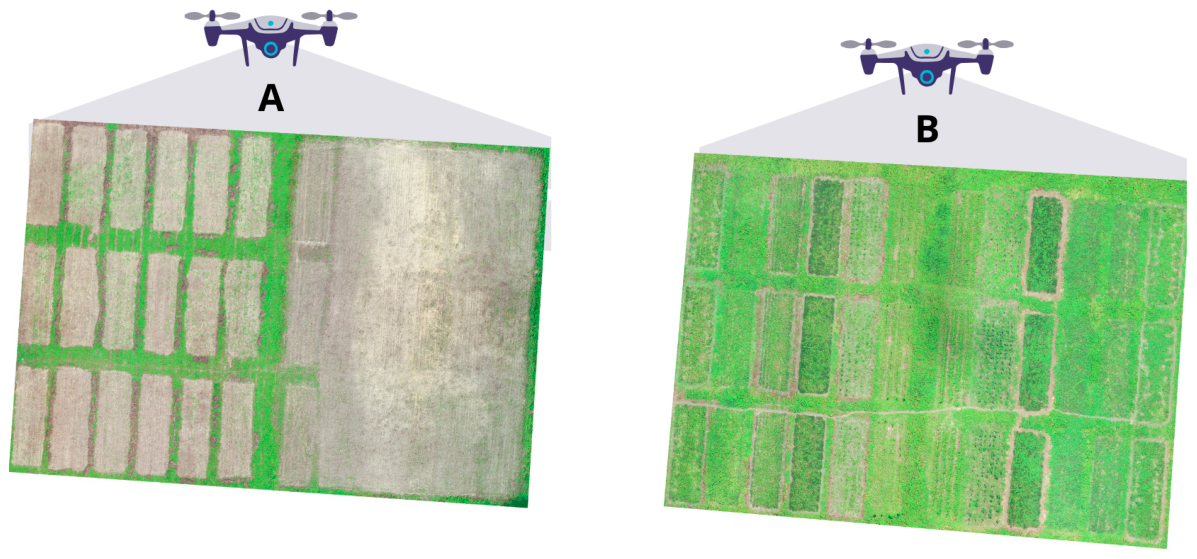
The orthomosaics generated from the UAV flights over the experimental peanut plots at two different time points (Figure 3) had dimensions of 9773 × 7591 pixels, providing a broad and detailed coverage of the study area. With a cell size of 0.01657 × 0.01657 m, the resulting spatial resolution was approximately 1.6 cm per pixel, which is suitable for capturing fine-scale plot details and for performing basic spectral analyses [52].
The orthomosaics consist of a three-band RGB spectral composition (red, green, and blue) with a radiometric resolution of 8 bits per pixel. This means that each pixel can take intensity values in the range 0–255, which is appropriate for visualization-based analyses and for computing vegetation indices that rely on these bands [53].

3.2. Spectral Indices Predictive of Soil Properties and Peanut Crop Traits

3.2.1. RGB Spectral Index Calculations

Of the 17 indices analyzed, the vNDVI, TGI, VEG, GLI, RGBVI, MGRVI, and VIgreen indices can be grouped as vegetation indices (VIs), that are commonly used to assess crop vigor due to their ability to capture vegetation reflectance.
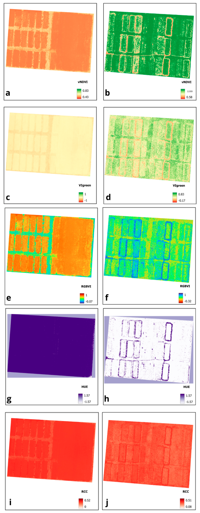
The vNDVI showed values ranging from 0.422 to 0.833, while TGI reached near-neutral values, from −4.40 to 24.91; VEG attained maximum values of 0.91, and GLI ranged between −0.213 and −0.078. The RGBVI and MGRVI indices also presented negative values, and VIgreen exhibited values close to −0.091 among the different treatments (Figure 4).
The low reflectance values observed during the initial stage can be explained by three concurrent factors. First, the first UAV flight was conducted during the early vegetative stage (0–15 days after sowing), when canopy cover was minimal and the spectral signal was dominated by bare-soil background rather than vegetation [54]. Under these conditions, RGB-based vegetation indices—particularly those sensitive to green biomass such as vNDVI, VIgreen, and GLI—naturally yield low or near-zero values, as they are designed to detect active chlorophyll-bearing canopy rather than exposed soil [55]. Second, indices such as RGBVI and MGRVI are known to produce negative values when the red band dominates over the green band, which is characteristic of bare or sparsely vegetated soils where no near-infrared reflectance is available to enhance the vegetation signal [56]. Third, the 8-bit radiometric resolution of the RGB sensor limits the dynamic range available for distinguishing subtle spectral contrasts in early-stage canopies, further compressing index values toward neutral or low magnitudes [54]. These conditions are consistent with the literature reporting that RGB spectral indices show highly stage-dependent performance, with their discriminative capacity substantially reduced when green canopy cover is below approximately 30% [54,55,56].
In the harvest phase, the VIs exhibited a marked increase in their mean reflectance values (Table A5 Appendix Mean spectral index values from first flight mission). The most pronounced increment was observed for TGI, which reached a maximum value of 121.14, while VEG and GLI also increased substantially, attaining maximum values of 1.69 and 0.40, respectively.
Similarly, vNDVI and VIgreen showed considerable increases, with maximum values of 0.996 and 0.999, respectively. However, these values are not characteristic of a fully vigorous canopy because the orthomosaic used for the analysis was acquired when the crop was approximately 72 days after germination, corresponding to the harvest stage, at which point the crop was no longer at its peak vigor (Table A6, Appendix).
Conversely, indices such as WI and ExB were sensitive to soil-related characteristics, including bulk density, moisture conditions, and blue-band reflectance. The decrease in WI between phenological stages, from −75 to −87, likely reflects changes in soil–water status driven by crop cover and activity, whereas ExB, being associated with the proportion of blue reflectance, emerges as a useful indicator of the physical properties of bare soil [57].
The analysis of RGB spectral indices across different phenological stages of the crop highlights their capacity to discriminate between bare soil and vegetation cover, as well as their utility for monitoring crop development. Indices such as vNDVI, VIgreen, and TGI proved to be highly sensitive tools for detecting changes in plant biomass between bare-soil conditions and maximum canopy cover [58], underscoring the feasibility of assessing crop status using only standard RGB cameras, which reduces costs and enhances the accessibility of these techniques in agricultural contexts. In this regard, previous studies, such as those by Pacheco and Montilla (2020) [59], have emphasized the usefulness of these RGB-based indices for applications under diverse agricultural conditions.

3.2.2. Distribution Analysis of Study Variables

The normality analysis performed using the Shapiro–Wilk test on 32 variables, including soil properties, crop morphological traits, and spectral indices, revealed that most of the data did not follow a normal distribution. Of the 32 variables evaluated, only 7 (CLF, NDT, Dr, Pr, WI, HUE, RCC) exhibited p-values above the 0.05 significance threshold, indicating that the null hypothesis of normality could not be rejected for these variables, whereas the remaining 25 variables showed p-values below 0.05, suggesting non-normal distributions.
The non-normal variables included edaphic measurements such as bulk density (SBD), field capacity moisture ( θ F C ), and Electrical Conductivity (EC), as well as spectral indices such as ExB, GR, and MGRVI. The high proportion of non-normal data led to the use of Spearman’s rank correlation, a nonparametric method, to assess the relationships among variables. This approach is particularly suitable for non-normally distributed data and allows robust estimation of associations without assuming normality, facilitating the identification of spectral indices with the greatest predictive potential for soil and morphological variables. It should be noted that the choice of correlation method was made on a variable-by-variable basis, according to the distributional properties identified through the Shapiro–Wilk test: Spearman’s rank correlation was applied to all variables that did not satisfy the normality assumption (p < 0.05), whereas Pearson’s correlation was used for variables that did meet the normality criterion (p ≥ 0.05) (Table A3, Appendix), namely crop chlorophyll content (CL; p = 0.430) and nodule weight (NW; p = 0.064) (Table A4, Appendix).

3.2.3. Spectral-Soil Relationships: RGB-Based Indices as Predictors of Bulk Density, Porosity, Moisture, and Organic Matter

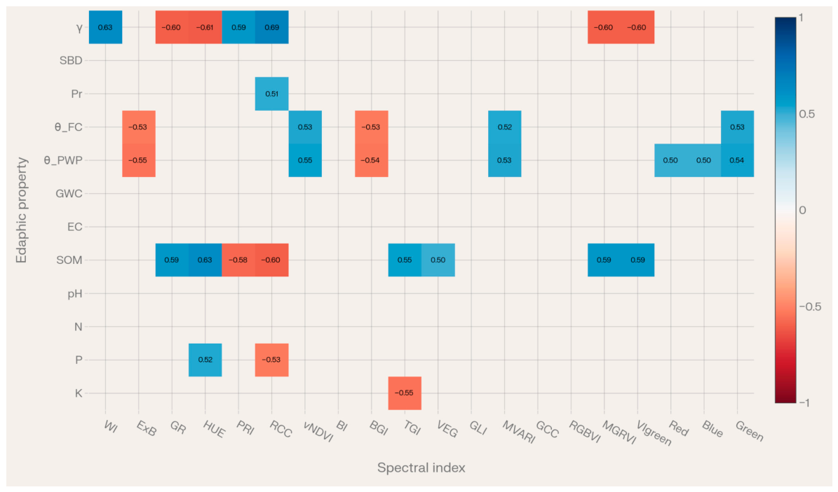
As shown in Figure 5, the correlation analysis revealed that the spectral indices exhibited significant associations with the soil bulk density (SBD). A strong positive correlation was observed between γ and the WI (r = 0.63), PRI (r = 0.59), and RCC (r = 0.69) indices. In contrast, strong negative correlations were identified between SBD and the GR (r = −0.60), HUE (r = −0.61), MGRVI (r = −0.60), and VIgreen (r = −0.60) indices.
Bulk density (SBD), which is directly related to soil compaction, explains its correlation with spectral indices through the way compaction alters the soil’s ability to reflect, absorb, and scatter light in the visible (RGB) bands. More compacted soils, characterized by closer particle packing and reduced pore space, markedly modify the optical properties of the soil surface [60]. In the green (G) and blue (B) bands, lower reflectance is typically observed due to reduced surface roughness and decreased water retained in pores, conditions that tend to become more homogeneous under compaction [57]. In contrast, the red (R) band tends to show higher reflectance, often associated with lower organic matter content and a lighter soil color as compaction increases. These spectral variations highlight the sensitivity of spectral indices to structural changes in the soil, positioning them as promising tools for diagnosing compaction-related constraints in agricultural systems [59].
Soil porosity (Pr) showed a strong positive correlation with the RCC index (ρ = 0.51), indicating that more porous soils exhibit distinctive optical characteristics in the visible spectrum. Highly porous soils, such as sandy textures, tend to reflect more light due to their lower water and organic matter retention, and RCC captures these differences by emphasizing variations in bare-soil exposure and surface composition [57].
Field capacity moisture ( θ F C ) displayed strong positive correlations with vNDVI (ρ = 0.53), MVARI (ρ = 0.52), and the green band reflectance (ρ = 0.53), underscoring the sensitivity of these indices to water stored in soil pores, which generally reduces reflectance in the green and red bands. Similar strong positive correlations between permanent wilting point moisture ( θ P W P ) and the same indices (ρ between 0.53 and 0.55) reinforce their suitability for detecting critical moisture levels in dry soils. Conversely, the strong negative correlations found with ExB (ρ = −0.55) and BGI (ρ = −0.54) suggest that these indices are less effective under high-moisture conditions, likely because they are designed to respond to higher blue and green reflectance, typical of drier soils [61].
Soil organic matter (SOM) exerts a critical influence on soil reflectance, particularly in the visible region, due to its dark color, high water-holding capacity, and impact on soil texture and structure. Soils rich in SOM generally exhibit lower reflectance, especially in the red and green bands, as SOM enhances light absorption at these wavelengths. This pattern is consistent with the results obtained, where HUE (ρ = 0.63), MGRVI, VIgreen, and TGI (ρ between 0.55 and 0.59) showed strong positive correlations, highlighting their capacity to capture the influence of SOM on soil reflectance, particularly in the green band, which is highly sensitive to darker tones associated with SOM-rich soils. In contrast, PRI (ρ = −0.58) and RCC (ρ = −0.60) exhibited strong negative correlations, suggesting that these indices respond inversely to increasing SOM content, likely due to enhanced absorption and reduced visible reflectance as SOM increases. This behavior can be explained by the greater light absorption in soils with high organic matter content, which alters the spectral response and reduces reflectance in the visible bands [62].
Taken together, these findings support the use of RGB-based indices as rapid, cost-effective, and operationally practical tools for assessing key soil physical properties and surface conditions. While the correlations observed with certain soil variables suggest a potential capacity to indirectly reflect surface-level variability associated with soil composition, these results should be interpreted with caution: the present study did not include a comprehensive independent soil chemical analysis, and therefore the indices should be regarded as exploratory proxies rather than validated predictors of soil chemical attributes. Their implementation can nonetheless enhance soil monitoring in agricultural systems, particularly in regions with limited laboratory infrastructure, as their sensitivity to spectral variations linked to soil structure, surface moisture, and organic matter dynamics makes them valuable, accessible tools for promoting more sustainable and data-informed agricultural practices. Future work integrating UAV-RGB indices with dedicated soil chemical sampling would help confirm and strengthen these associations. [63].
It is worth noting that the spectral-soil relationships described above encompass both tillage systems evaluated in this study, zero tillage (ZT, treatments T1–T8) and conventional tillage (CT, treatments T9–T16), which generate measurably different surface conditions that influence the spectral response of the soil. Under ZT, the absence of mechanical soil disturbance preserves greater surface heterogeneity, including residual crop material, surface organic matter, and a more stable soil aggregate structure. This is reflected in the spectral data: ZT treatments (e.g., T3 and T4) showed slightly higher values in chromatic indices such as HUE and GR, which are sensitive to darker surface tones associated with higher surface organic matter content (Table A3, Appendix). In contrast, CT treatments (T9–T16) produced more homogeneous and brighter soil surfaces due to mechanical inversion, resulting in higher red-band reflectance and slightly lower vNDVI values, consistent with reduced organic matter exposure and increased soil particle uniformity after plowing. Vegetation-sensitive indices such as RGBVI and VIgreen also showed moderate inter-treatment variability between the two tillage systems, reflecting differences in the soil-to-canopy proportion during the early crop stage, when ground cover is still incomplete. These contrasting spectral behaviors reinforce the idea that tillage-induced surface modifications are partially detectable through RGB-based indices, and that the observed variability in the spectral-soil correlations is, at least in part, attributable to the differential surface conditions generated by each soil management system. Nonetheless, it should be emphasized that the primary objective of this study was to evaluate the potential of UAV-RGB-derived indices for detecting spatial variability in crop and soil conditions, with the tillage system treated as a contributing factor to the overall spectral variability rather than the primary subject of comparison.

3.3. Spectral Indices Associated with Crop Physiological Traits

Variables Physiological Variables of the Peanut Crop

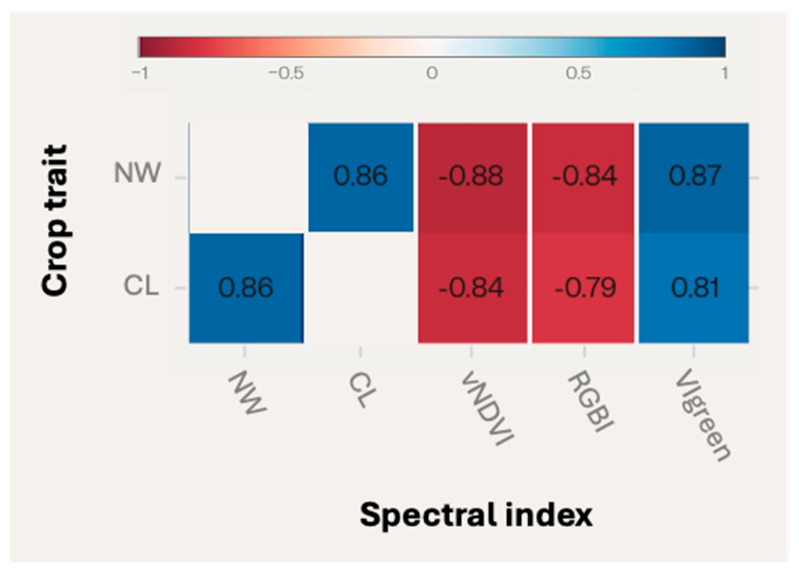
As shown in Figure 6, the Pearson correlation analysis between spectral indices and the crop variables CL and NW, both of which satisfied the normality assumption (Shapiro–Wilk test, p ≥ 0.05; Table A2, Appendix), revealed significant patterns that highlight the interaction between the crop’s biochemical properties and its spectral response. The very strong positive correlation between chlorophyll content (CL) and nodule weight (NW) (ρ = 0.86) indicates that higher photosynthetic activity promotes nodule development, reflecting a direct metabolic relationship. However, chlorophyll content showed strong negative correlations with vNDVI (ρ = −0.88) and RGBVI (ρ = −0.84), which can be attributed to reduced absorption in the red and blue bands during the late growth stage, when chlorophyll levels are low [64]. These conditions also affect NW, which exhibited negative correlations with vNDVI (ρ = −0.84) and RGBVI (ρ = −0.79), underscoring the influence of nodular metabolism on the spectral reflectance of the crop.
Conversely, VIgreen exhibited a strong positive correlation with both chlorophyll content (CL) (ρ = 0.84) and nodule weight (NW) (ρ = 0.81), as it emphasizes the green band, which is less affected by the decline in chlorophyll during the late stages of crop development [65]. These results underscore the importance of accounting for phenological stage and crop physiological interactions when interpreting spectral indices in peanut systems, where biochemical and spectral variables are tightly coupled.

3.4. Predictive Modeling of Soil and Crop Properties from RGB-Based Spectral Indices

3.4.1. Spectral-Based Soil Property Modeling

The performance metrics reported in Table 4 and Table 5 (R2, RMSE, and MAE) refer to the predictions obtained on the independent test set, which comprised 30% of the total dataset. Model hyperparameters were first tuned using five-fold cross-validation on the remaining 70% training set, and the final models—fitted with the optimal hyperparameters—were then evaluated on the test set. Thus, all values shown in these tables correspond to out-of-sample performance and provide a robust assessment of the predictive capability of each model configuration.
As shown in Table 4, the regression analysis using the Random Forest (RF) algorithm outperformed the k-Nearest Neighbors (KNN) model. The RF model relating the RGBVI index to soil bulk density (SBD) achieved a strong association, with a coefficient of determination of R 2 = 0.58 between predicted and observed values. However, the resulting mean squared error (MSE = 20.47) and mean absolute error (MAE = 4.2) were relatively high, indicating that the predictions deviate substantially from the measured values and suggesting considerable variability in the model estimates [66].
On the other hand, the Random Forest model linking vNDVI to soil bulk density (SBD) also yielded a relatively high coefficient of determination (R2 = 0.70). However, the elevated MSE (14.37) and MAE (3.51) values reveal considerable dispersion between predictions and observations, which undermines the effective predictive capability of the model despite the statistically significant association.
The Random Forest model using the HUE (Overall Hue Index) to estimate soil organic matter (SOM) showed a strong relationship, with R2 = 0.62, together with lower MSE (0.11) and MAE (0.27) values, supporting the robustness of this index for SOM prediction by indicating reduced variability between predicted and measured values [67]. In a similar way, the model based on the RCC (Red Chromatic Coordinate) index for SOM prediction achieved the highest coefficient of determination (R2 = 0.87), with MSE = 0.04 and MAE = 0.18. These results indicate that the predictions produced by this model are very close to the observed values, with negligible variability [67,68]; therefore, this approach emerges as an optimal tool for estimating soil organic matter content from RGB imagery.

3.4.2. Machine Learning for Chlorophyll Assessment

In the regression results obtained with the Random Forest (RF) algorithm, the predictive performance for chlorophyll content (CL) and nodulation (NW) based on the RGBVI, vNDVI, and VIgreen spectral indices was highly variable (Table 5). The RF model relating vNDVI to CL showed a strong association (R2 = 0.51) between predicted and observed values, with an MSE of 0.01 and an MAE of 0.09, indicating low variability and small average error. This model is therefore considered the most suitable for estimating chlorophyll content under the conditions evaluated, consistent with previous studies reporting strong correlations between indices that emphasize differences between the red and green bands and chlorophyll content due to the strong absorption of red light by chlorophyll [64,69].
The RF model relating VIgreen to CL also showed a strong correlation (R2 = 0.73), indicating substantial predictive capability. However, the high MSE (13.2) and MAE (3.18) values suggest considerable variability in the predictions, possibly due to the presence of outliers or the need for further model optimization [70].
By contrast, the models computed with the KNN algorithm yielded only moderate to low correlation values between CL and the RGBVI, vNDVI, and VIgreen indices (Table 6), which reinforces the superior performance of RF in this context.
These findings reinforce the usefulness of RGB spectral indices for non-destructive estimation of physiological variables in agronomic studies. The vNDVI emerged as the most robust index for predicting chlorophyll content, in agreement with previous research highlighting its ability to capture vegetation dynamics using conventional RGB imagery [71,72]. Furthermore, the results show that Random Forest clearly outperforms KNN in terms of predictive capacity and accuracy [73]. The robustness of RF to nonlinear relationships and its relative resistance to overfitting make it particularly suitable for complex problems such as predicting soil properties from spectral indices [74].
In contrast, KNN, although simple and effective in certain applications, failed to adequately capture the complexity of the relationships among variables in this study, especially for predicting SBD and SOM. The low R2 values and high MSE and MAE observed in most KNN models indicate that this algorithm is not the most appropriate choice when data variability and nonlinear relationships play a critical role [75].

3.5. Methodological Limitations and Future Research Directions

The findings of this study are conditioned by several methodological aspects that should be considered when extrapolating the results. First, all spectral information was derived from 8-bit RGB imagery acquired under specific illumination and atmospheric conditions, which makes the derived indices sensitive to variations in solar angle, shadows, and sensor calibration. This can introduce noise into the reflectance signal, particularly in the blue band, and partially explains the relatively high MSE and MAE observed in some models despite acceptable R2 values [76].
Second, RGB-based vegetation indices inherently lack near-infrared and red-edge information, which are known to increase sensitivity to biomass, canopy structure, and plant water status [77]. As a result, the predictive models developed here are best interpreted as proxies calibrated for the specific phenological stages, soil background, and management conditions of the peanut system studied, rather than as universally transferable relationships. Third, the sample size and the spatial extent were constrained to experimental plots within a single growing season, which limits the capacity to capture interannual climate variability and broader edaphic gradients [78].
In addition, the machine learning models were trained on datasets with a relatively high proportion of non-normal variables and potential outliers, which, although handled through nonparametric statistics and robust algorithms such as Random Forest, may still contribute to residual uncertainty in the predictions [79]. Importantly, these constraints do not undermine the relevance of the results; instead, they highlight clear avenues for future work, including (i) multi-year and multi-site validations across contrasting soil types and management systems, (ii) integration of multispectral or hyperspectral data with RGB indices to improve sensitivity and reduce saturation effects, and (iii) coupling of UAV-based observations with satellite time series and geospatial decision-support systems to scale the methodology from experimental plots to operational farm and landscape levels [80].

3.6. Geospatial Technologies and the Transformation of Rural Agriculture in Manabí, Ecuador

The empirical results of this study must be interpreted within the broader socio-territorial context of rural Ecuador, and particularly of the province of Manabí, where agriculture remains a key livelihood under conditions of structural vulnerability. Recent assessments indicate that approximately 43.2% of Ecuador’s rural population lives below the national poverty line, with Manabí among the provinces with the highest numbers of people facing acute food insecurity and underemployment. Rural communities in Manabí often experience limited access to quality education, technical assistance, irrigation infrastructure, and digital connectivity, which constrains their capacity to adopt improved agronomic practices and to respond to climate and market shocks [81].
In this setting, the deployment of geospatial technologies—such as UAV- and satellite-based remote sensing, GIS, and AI-driven decision-support systems—offers a strategic pathway to strengthen agro-productive systems and local governance [82]. International experiences in Latin America show that integrating GPS, GIS, and remote sensing into precision agriculture can optimize input use, reduce environmental impacts, and increase profitability, especially when tools are adapted to smallholder realities and embedded in collaborative extension schemes. Initiatives that couple field data, satellite analytics, and machine learning have already demonstrated their potential to generate operational crop monitoring layers (e.g., yield, water stress, soil fertility) for smallholder systems, enabling more targeted public support and private investment [83].
For territories like Manabí, RGB-based indices and low-cost UAV platforms, as explored in this work, represent an accessible entry point into geospatial innovation. When integrated into municipal or provincial geoportals and agricultural information systems, such indices could support early-warning tools for drought or pest outbreaks, spatially explicit fertilizer and lime recommendations, and evidence-based land-use planning. This, in turn, would facilitate a more transparent and technically grounded dialog between local governments, producer organizations, and extension services, aligning with global trends in which geospatial infrastructures underpin sustainable, climate-smart, and socially inclusive agricultural transitions [84].

4. Conclusions

The UAV-derived orthomosaics, with a spatial resolution of 1.6 cm per pixel and 8-bit RGB bands, enabled detailed spectral analyses, supporting precise monitoring of peanut plots and more informed agronomic decision-making.
The use of RGB-based indices demonstrated the feasibility of advanced crop and soil assessments relying solely on standard RGB cameras, thereby reducing costs and improving technological accessibility for precision agriculture.
The study showed that the Random Forest (RF) algorithm outperformed k-Nearest Neighbors (KNN) for predicting soil properties from RGB spectral indices. Among the tested indices, RCC achieved the highest accuracy for soil organic matter (SOM) estimation, with a coefficient of determination of R2 = 0.87 and low error values (MSE = 0.04, MAE = 0.18), highlighting its robustness as a proxy indicator of SOM.
Regression results using RF also underscored its superiority for predicting plant chlorophyll content. The vNDVI-based model showed the strongest association with chlorophyll (R2 = 0.51), combined with low MSE (0.01) and MAE (0.09), indicating good predictive skill. In contrast, although VIgreen yielded a higher R2 (0.73), its much larger MSE (13.2) and MAE (3.18) revealed substantial prediction variability, likely driven by outliers or phenological effects.
Overall, RF consistently outperformed KNN for predicting both soil and crop properties from RGB spectral indices. RF provided higher predictive power and lower error metrics, reflecting its ability to capture nonlinear relationships and handle data variability, whereas KNN struggled to model the complex interactions present in bulk density, SOM, and physiological variables. This advantage positions RF as the most suitable approach for tackling agronomic prediction problems based on RGB-derived indices.
The results of this study demonstrate that RGB-derived indices such as RCC, OHI, vNDVI, and VIgreen are viable and effective tools for predicting both crop and soil attributes. Their capacity to capture spectral reflectance variations associated with key characteristics—including chlorophyll content, soil bulk density, and SOM—highlights their value for agronomic applications. Despite the inherent variability in some models, RGB indices offer a rapid, non-destructive, and accessible alternative for monitoring and estimating critical soil and crop properties, making them a promising option to support improved agricultural management and decision-making in the field.

Author Contributions

Conceptualization, E.Z.-L. and H.A.P.G.; methodology, W.S.-A., C.D.-M. and H.A.P.G.; software, C.D.-M.; validation, C.A.R., E.Z.-L. and H.A.P.G.; formal analysis, W.S.-A. and C.D.-M.; investigation, E.Z.-L., W.S.-A. and C.D.-M.; resources, E.Z.-L. and H.A.P.G.; data curation, W.S.-A. and C.A.R.; writing—original draft preparation, W.S.-A. and C.D.-M.; writing—review and editing, E.Z.-L., H.A.P.G. and C.A.R.; visualization, C.D.-M. and W.S.-A.; supervision, E.Z.-L. and H.A.P.G.; project administration, E.Z.-L. and H.A.P.G.; All authors have read and agreed to the published version of the manuscript.

Funding

This research received no external funding.

Institutional Review Board Statement

Not applicable.

Informed Consent Statement

Not applicable.

Data Availability Statement

The original contributions presented in this study are included in the article. Further inquiries can be directed to the corresponding authors.

Conflicts of Interest

The authors declare no conflicts of interest.

Abbreviations

The following abbreviations are used in this manuscript:
AIArtificial Intelligence
SBDBulk Density
BGISimple Blue–Green Ratio/Blue–Green Pigment Index
BIBrightness Index
CLChlorophyll content (in leaves)
CMOSComplementary Metal-Oxide-Semiconductor (sensor type)
CPPercentage of Clay Particles
DLDeep learning
DSMDigital Surface Model
DSTsDecision-Support Tools
DTMDigital Terrain Model
ECElectrical Conductivity
ESPACContinuous Agricultural Area and Production Survey
ExBExcess Blue Index
FAOFood and Agriculture Organization
θ FCField capacity moisture content
GCCGreen Percentage Index
GLIGreen Leaf Index
GNSS RTKGlobal Navigation Satellite System—Real-Time Kinematic
GRSimple Red–Green Ratio
GWCGravimetric Water Content
HUEOverall Hue Index
INIAPNational Institute of Agricultural Research
KPotassium
KNNk-Nearest Neighbors
LCConventional tillage
L0Zero tillage
M1Planting Density 1 (62,500 plants/ha)
M2Planting Density 2 (100,000 plants/ha)
MAEMean absolute error
MGRVIModified Green–Red Vegetation Index
MSEMean squared error
MVARIModified Visible Atmospherically Resistant Vegetation Index
NTotal nitrogen
NDVINormalized Difference Vegetation Index
NWNodule weight
SOMSoil organic matter
PPhosphorus
pHPotential of Hydrogen
PRIPhotochemical Reflectance Index
PrPorosity
θ_PWPPermanent wilting point
RCCRed Chromatic Coordinate Index
RFRandom Forest
RGBRed, Green, Blue (spectral bands)
RGBVIRed–Green–Blue Vegetation Index
RMSERoot mean square error
SBDSoil bulk density
SISpectral index
SIsSpectral indices
SiPPercentage of Silt Particles
SiPc1Bouyoucos hydrometer reading corrected at 40 s
SiPc2Bouyoucos hydrometer reading corrected at 2 h
SPPercentage of Sand Particles
TGITriangular Greenness Index
TNTotal nitrogen
UAVUnmanned aerial vehicle
UTMUniversal Transverse Mercator (coordinate system)
V1-V4Peanut varieties (INIAP 381, 383, 380, 382)
VIgreenVegetation Index Green
vNDVIvisible Normalized Difference Vegetation Index
WIWoebbecke Index
γ (gamma)Particle density (real density)
ΓwaterSpecific weight of distilled water

Appendix A. Experimental Design: Treatment Combinations for Peanut Crop Trial

This appendix details the factorial structure of the experimental design used in the study, comprising 16 treatments derived from the interaction of four factors: peanut varieties (V1-V4: INIAP 381 ROSITA, INIAP 383 Pintado, INIAP 380 Charapoto, INIAP 382 Caramelo), planting densities (M1: 62,500 plants/ha; M2: 100,000 plants/ha), and tillage systems (L0: zero tillage; LC: conventional tillage). These supplemental details enable exact reproduction of the trial without disrupting the main text flow and include raw treatment configuration data for subsequent analyses.
Table A1. Treatment description (T1 to T14).
TratamientosFactor AFactor BFactor CInteracción
T1V1: INIAP 381 ROSITAM1: 62,500 plants/ha (0.2 m × 0.8 m)L0: zero tillageV1 M1 L0
T2V1: INIAP 381 ROSITAM2: 100,000 plants/ha (0.2 m × 0.5 m)V1 M2 L0
T3V2: INIAP 383 PintadoM1: 62,500 plants/ha (0.2 m × 0.8 m)V2 M1 L0
T4V2: INIAP 383 PintadoM2: 100,000 plants/ha (0.2 m × 0.5 m)V2 M2 L0
T5V3: INIAP 380 CharapotoM1: 62,500 plants/ha (0.2 m × 0.8 m)V3 M1 L0
T6V3: INIAP 380 CharapotoM2: 100,000 plants/ha (0.2 m × 0.5 m)V3 M2 L0
T7V4: INIAP 382 CarameloM1: 62,500 plants/ha (0.2 m × 0.8 m)V4 M1 L0
T8V4: INIAP 382 CarameloM2: 100,000 plants/ha (0.2 m × 0.5 m)V4 M2 L0
T9V4: INIAP 382 CarameloM1: 62,500 plants/ha (0.2 m × 0.8 m)LC: conventional tillageV4 M1 LC
T10V4: INIAP 382 CarameloM2: 100,000 plants/ha (0.2 m × 0.5 m)V4 M2 LC
T11V3: INIAP 380 CharapotoM1: 62,500 plants/ha (0.2 m × 0.8 m)V4 M1 LC
T12V3: INIAP 380 CharapotoM2: 100,000 plants/ha (0.2 m × 0.5 m)V4 M2 LC
T13V2: INIAP 383 PintadoM1: 62,500 plants/ha (0.2 m × 0.8 m)V4 M1 LC
T14V2: INIAP 383 PintadoM2: 100,000 plants/ha (0.2 m × 0.5 m)V4 M2 LC
T15V1: INIAP 381 ROSITAM1: 62,500 plants/ha (0.2 m × 0.8 m)V4 M1 LC
T16V1: INIAP 381 ROSITAM2: 100,000 plants/ha (0.2 m × 0.5 m)V4 M2 LC

Appendix B. Statistical Analyses

This appendix provides detailed statistical outputs supporting the main text analyses, including normality testing via Shapiro–Wilk, Spearman’s rank correlations between vegetation indices and edaphic properties, and correlations between vegetation indices and crop properties (chlorophyll content—CL; nodule weight—NW). These results justify the use of non-parametric methods due to prevalent non-normality in agricultural spectral data.
Table A2. Shapiro–Wilk normality test results. CL = chlorophyll; NW = nodule weight; γ = the real density; SBD = soil bulk density; Pr = porosity; θ F C = field capacity moisture conten; θ P W P = the permanent wilting point moisture content; GWC = Gravimetric Water Content; EC = Electrical Conductivity; N = total nitrogen; P = potassium; K = phosphorus; SOM = soil organic matter; WI = Woebbecke Index; ExB = Excess Blue; GR = Simple Red–Green Ratio; HUE = Overall Hue Index; PRI = Photochemical Reflectance Index; RCC = Red Chromatic Coordinate Index; vNDVI = visible NDVI; BI = Brightness Index; BGI = Simple Blue–Green Ratio/Blue–Green Pigment Index; TGI = Triangular Greenness Index; VEG = Vegetative Index; GLI = Green Leaf Index; MVARI = Modified Visible Atmospherically Resistant Vegetation Index; GCC = Green Percentage Index; RGBVI = Red–Green–Blue Vegetation Index; MGRVI = Modified Green–Red Vegetation Index; VIgreen = Vegetation Index Green; Red, Green, Blue = band reflectance values.
Variablep-ValueNormality
CL0.430Normal
NW0.064Normal
γ 0.071Normal
SBD0.000No normal
Pr0.213Normal
θ F C 0.011No normal
θ P W P 0.010No normal
GWC0.022No normal
EC0.000No normal
pH0.002No normal
N0.000No normal
P0.002No normal
K0.000No normal
SOM0.000No normal
WI0.068Normal
ExB0.000No normal
GR0.008No normal
HUE0.639Normal
PRI0.000No normal
RCC0.639Normal
vNDVI0.467Normal
BI0.012No normal
BGI0.013No normal
TGI0.026No normal
VEG0.041No normal
GLI0.043No normal
MVARI0.016No normal
GCC0.016No normal
RGBVI0.012No normal
MGRVI0.014No normal
VIgreen0.570Normal
RI0.563Normal
Green0.603Normal
Table A3. Spearman Correlation Matrix—vegetation indices vs. edaphic properties. γ = the real density; SBD = soil bulk density; Pr = porosity; θ F C = field capacity moisture conten; θ P W P = the permanent wilting point moisture content; GWC = Gravimetric Water Content; EC = Electrical Conductivity; N = total nitrogen; P = potassium; K = phosphorus; SOM = soil organic matter; WI = Woebbecke Index; ExB = Excess Blue; GR = Simple Red–Green Ratio; HUE = Overall Hue Index; PRI = Photochemical Reflectance Index; RCC = Red Chromatic Coordinate Index; vNDVI = visible NDVI; BI = Brightness Index; BGI = Simple Blue–Green Ratio/Blue–Green Pigment Index; TGI = Triangular Greenness Index; VEG = Vegetative Index; GLI = Green Leaf Index; MVARI = Modified Visible Atmospherically Resistant Vegetation Index; GCC = Green Percentage Index; RGBVI = Red–Green–Blue Vegetation Index; MGRVI = Modified Green–Red Vegetation Index; VIgreen = Vegetation Index Green; Red, Green, Blue = band reflectance values.
WIExBGRHUEPRIRCCvNDVIBIBGITGIVEGGLIMVARIGCCRGBVIMGRVIVIgreenRedBlueGreen
γ 0.63−0.13−0.60−0.610.590.690.180.090.00−0.44−0.46−0.35−0.06−0.35−0.35−0.60−0.600.330.140.11
SBD0.04−0.02−0.05−0.060.040.060.010.11−0.04−0.11−0.04−0.020.16−0.02−0.03−0.04−0.040.100.110.07
Pr0.49−0.11−0.44−0.440.430.510.160.040.00−0.28−0.32−0.24−0.10−0.24−0.24−0.44−0.430.230.080.07
θ F C 0.40−0.530.170.21−0.180.100.530.49−0.530.230.320.400.520.400.400.180.180.490.490.53
θ P W P 0.41−0.550.180.22−0.190.090.550.49−0.540.240.330.420.530.410.410.180.190.500.500.54
GWC−0.420.030.420.45−0.41−0.44−0.07−0.19−0.070.360.330.270.140.270.270.410.41−0.32−0.22−0.17
EC0.310.00−0.30−0.360.290.310.030.160.07−0.29−0.25−0.20−0.14−0.20−0.20−0.30−0.300.250.190.14
SOM−0.49−0.020.590.63−0.58−0.60−0.03−0.15−0.130.550.500.420.120.420.420.590.59−0.34−0.21−0.13
pH0.070.27−0.33−0.430.310.19−0.24−0.070.32−0.42−0.36−0.36−0.37−0.36−0.36−0.32−0.320.050.03−0.06
N−0.16−0.050.220.22−0.22−0.200.030.00−0.110.190.200.180.160.180.170.220.22−0.09−0.05−0.02
P−0.440.050.480.52−0.47−0.53−0.09−0.05−0.030.380.390.30−0.010.310.310.480.48−0.21−0.06−0.03
K0.150.25−0.46−0.450.460.35−0.220.100.31−0.55−0.47−0.45−0.28−0.45−0.45−0.46−0.460.170.130.01
Table A4. Pearson Correlation Matrix—vegetation indices vs. crop properties. CL = chlorophyll; NW = nodule weight; WI = Woebbecke Index; ExB = Excess Blue; GR = Simple Red–Green Ratio; HUE = Overall Hue Index; PRI = Photochemical Reflectance Index; RCC = Red Chromatic Coordinate Index; vNDVI = visible NDVI; BI = Brightness Index; BGI = Simple Blue–Green Ratio/Blue–Green Pigment Index; TGI = Triangular Greenness Index; VEG = Vegetative Index; GLI = Green Leaf Index; MVARI = Modified Visible Atmospherically Resistant Vegetation Index; GCC = Green Percentage Index; RGBVI = Red–Green–Blue Vegetation Index; MGRVI = Modified Green–Red Vegetation Index; VIgreen = Vegetation Index Green; Red, Green, Blue = band reflectance values.
NWCLWIExBGRHUEPRIRCCvNDVIBIBGITGIVEGGLIMVARIGCCRGBVIMGRVIVIgreenRedBlueGreen
NW1.000.86−0.12−0.21−0.17−0.040.060.17−0.88−0.27−0.23−0.260.030.250.110.06−0.84−0.060.87−0.15−0.23−0.37
CL0.861−0.23−0.20−0.14−0.140.140.25−0.84−0.18−0.22−0.06−0.020.310.060.01−0.79−0.140.81−0.04−0.17−0.31

Appendix C. Raw Spectral Data from UAV Orthomosaics

This appendix presents the raw mean values of RGB-based vegetation indices calculated from two UAV orthomosaic flights conducted during the peanut crop trial. These data supplement the main text by providing complete treatment-level measurements across 20 spectral indices, enabling detailed statistical replication and model validation without cluttering the primary results section.
Table A5. Mean spectral index values from first flight mission. Trt = treatments; WI = Woebbecke Index; ExB = Excess Blue; GR = Simple Red–Green Ratio; HUE = Overall Hue Index; PRI = Photochemical Reflectance Index; RCC = Red Chromatic Coordinate Index; vNDVI = visible NDVI; BI = Brightness Index; BGI = Simple Blue–Green Ratio/Blue–Green Pigment Index; TGI = Triangular Greenness Index; VEG = Vegetative Index; GLI = Green Leaf Index; MVARI = Modified Visible Atmospherically Resistant Vegetation Index; GCC = Green Percentage Index; RGBVI = Red–Green–Blue Vegetation Index; MGRVI = Modified Green–Red Vegetation Index; VIgreen = Vegetation Index Green; Red, Green, Blue = band reflectance values.
TrtWIExBGRHUEPRIRCCvNDVIBIBGITGIVEGGLIMVARIGCCRGBVIMGRVIVIgreenRedBlueGreen
T1−0.6900.1790.8340.3481.2010.3590.4291,034,199,997.5331.145−25.0650.844−0.078−0.1520.299−0.155−0.180−0.091188.700179.373157.946
T2−0.7420.1850.8280.3311.2100.3590.427967,928,989.6671.164−26.6100.836−0.084−0.1750.297−0.166−0.187−0.095185.486177.656154.100
T3−0.7430.1770.8520.3851.1740.3550.4291,164,435,276.6671.134−23.7970.859−0.071−0.1390.303−0.140−0.159−0.080193.341186.134165.148
T4−0.7500.1730.8660.4231.1560.3530.4311,215,051,238.6671.121−21.9910.871−0.064−0.1230.305−0.127−0.144−0.072194.424188.156168.609
T5−1.0190.1870.8700.4261.1500.3480.4251,196,772,870.3331.161−24.6810.865−0.071−0.1880.303−0.141−0.138−0.070190.481191.122166.191
T6−1.0080.1870.8710.4311.1490.3470.4261,182,931,347.6671.160−24.3630.866−0.071−0.1850.303−0.140−0.137−0.069189.706190.358165.741
T7−0.7240.1660.8820.4811.1340.3510.4331,300,487,940.0001.099−19.0830.887−0.055−0.0980.310−0.109−0.125−0.063196.846190.620173.965
T8−0.8300.1770.8740.4551.1460.3500.4291,243,307,257.6671.134−21.4620.875−0.064−0.1660.306−0.126−0.134−0.068192.821189.324169.226
T9−0.8080.1640.9000.5561.1120.3470.4341,639,958,516.6671.089−17.8860.901−0.048−0.0870.313−0.095−0.105−0.053205.996201.905185.614
T10−0.8190.1650.8960.5381.1160.3480.4331,650,891,523.6671.094−18.7050.898−0.050−0.0920.312−0.099−0.109−0.055206.184202.147185.017
T11−0.8530.1770.8680.4331.1540.3510.4291,384,809,676.3331.130−23.3260.869−0.066−0.1270.305−0.131−0.141−0.071197.374193.295171.560
T12−0.9040.1790.8700.4431.1520.3500.4281,193,450,980.8671.135−22.6230.870−0.066−0.1340.305−0.132−0.139−0.070189.611186.865165.313
T13−0.9700.1730.8900.5151.1240.3470.4301,029,552,207.8001.116−18.9120.888−0.056−0.1160.309−0.112−0.116−0.058182.117180.855162.435
T14−0.9790.1720.8940.5351.1200.3460.431979,848,965.1671.112−17.9310.891−0.055−0.1120.310−0.108−0.112−0.056179.153178.005160.522
T15−1.2420.1850.8880.5111.1290.3440.426725,036,481.7001.150−19.7070.878−0.064−0.1600.305−0.128−0.119−0.060164.279167.220146.366
T16−1.4670.1960.8870.4981.1310.3410.422685,633,857.4001.184−21.3510.870−0.072−0.2130.302−0.141−0.121−0.061160.183166.439142.648
Table A6. Mean spectral index values from second flight mission. Trt = treatments; WI = Woebbecke Index; ExB = Excess Blue; GR = Simple Red–Green Ratio; HUE = Overall Hue Index; PRI = Photochemical Reflectance Index; RCC = Red Chromatic Coordinate Index; vNDVI = visible NDVI; BI = Brightness Index; BGI = Simple Blue–Green Ratio/Blue–Green Pigment Index; TGI = Triangular Greenness Index; VEG = Vegetative Index; GLI = Green Leaf Index; MVARI = Modified Visible Atmospherically Resistant Vegetation Index; GCC = Green Percentage Index; RGBVI = Red–Green–Blue Vegetation Index; MGRVI = Modified Green–Red Vegetation Index; VIgreen = Vegetation Index Green; Red, Green, Blue = band reflectance values.
TrtWIExBGRHUEPRIRCCvNDVIBIBGITGIVEGGLIMVARIGCCRGBVIMGRVIVIgreenRedGreenBlue
T1−2.167−0.0891.303−0.3740.7810.3300.535575,652,562.1310.57660.1891.4490.0280.3500.4280.3830.2460.167141.026179.588105.570
T2−2.223−0.0941.310−0.3740.7760.3300.537566,292,328.1660.56662.4891.4580.3040.3580.4300.4030.2520.160141.226181.194104.306
T3−1.782−0.1321.444−0.2830.7040.3170.552563,557,674.7010.51376.7421.6090.2370.4080.4540.4710.3390.134134.227189.69399.348
T4−1.898−0.1241.408−0.3070.7230.3210.549628,511,128.0730.52475.3771.5730.2260.3960.4480.4930.3170.131139.991192.802102.997
T5−2.188−0.0741.286−0.3940.7890.3300.567591,992,364.8760.59757.8681.4130.1750.3370.4220.6600.2360.111142.970180.353109.388
T6−2.179−0.0741.280−0.3820.7940.3310.588554,415,861.6500.59855.6821.4100.1730.3350.4210.5800.2300.124139.883175.287106.640
T7−1.812−0.0951.374−0.3110.7380.3200.534357,305,022.6750.56557.9751.5000.2440.3700.4360.4140.2970.153119.937160.99692.207
T8−1.775−0.0781.325−0.3140.7660.3240.537424,924,977.4670.59055.5121.4430.2450.3480.4270.3510.2640.156127.853165.77999.023
T9−1.458−0.1011.456−0.2390.7000.3080.554436,262,488.6690.56064.8181.5670.2010.3860.4450.4190.3450.118120.533171.10397.174
T10−1.491−0.0961.445−0.2480.7050.3090.542487,911,246.8340.56666.4151.5520.2270.3810.4430.4420.3390.137125.370177.208101.473
T11−1.475−0.0961.455−0.2550.6960.3070.561610,690,134.9560.56771.8821.5570.1890.3830.4440.5090.3490.122133.923191.246110.055
T12−1.479−0.0971.457−0.2540.6950.3070.567590,511,387.4120.56471.3211.5610.1900.3840.4450.5580.3500.112132.355189.079108.424
T13−1.672−0.0821.396−0.2960.7260.3130.556597,626,848.7440.58567.0101.4970.2210.3640.4350.4060.3120.131137.571188.686111.513
T14−1.786−0.0711.356−0.3230.7490.3180.552618,009,600.7670.60263.7041.4530.2070.3470.4280.4110.2840.127141.564188.765114.509
T15−1.680−0.0971.414−0.2900.7190.3140.553640,574,359.6220.56571.3851.5320.1820.3770.4410.5050.3210.107139.674193.377110.687
T16−1.896−0.0931.364−0.3270.7470.3210.534664,630,252.5420.57068.1791.4920.2400.3650.4350.4060.2880.159143.854191.937110.910

References

  1. Al-Qubati, A.; Zhang, L.; Forkel, M. Urban and peri-urban agriculture under climate change: A review on carbon emissions and sequestration. Sustain. Cities Soc. 2024, 115, 105830. [Google Scholar] [CrossRef] [Scilit]
  2. Rodríguez, S.L.; van Bussel, L.G.; Alkemade, R. Classification of agricultural land management systems for global modeling of biodiversity and ecosystem services. Agric. Ecosyst. Environ. 2024, 360, 108795. [Google Scholar] [CrossRef] [Scilit]
  3. Mabhaudhi, T.; Dirwai, T.L.; Taguta, C.; Sikka, A.; Lautze, J. Mapping Decision Support Tools (DSTs) on agricultural water productivity: A global systematic scoping review. Agric. Water Manag. 2023, 290, 108590. [Google Scholar] [CrossRef] [Scilit]
  4. Tao, X.; Damron, E.; Silvestri, S. High-Precision Crop Monitoring Through UAV-Aided Sensor Data Collection. In Proceedings of the IEEE International Conference on Communications; IEEE: New York, NY, USA, 2024; pp. 3506–3511. [Google Scholar] [CrossRef] [Scilit]
  5. Ingole, R.S.; Ingole, N.S.; Khandelwal, R.R.; Kalambe, J.P. Detection of Crop Disease and Spraying of Pesticides Using Drone. In Proceedings of the 2024 IEEE 9th International Conference for Convergence in Technology, I2CT 2024; IEEE: New York, NY, USA, 2024; pp. 1–5. [Google Scholar] [CrossRef] [Scilit]
  6. Dorbu, F.; Hashemi-Beni, L. Detection of Individual Corn Crop and Canopy Delineation from Unmanned Aerial Vehicle Imagery. Remote Sens. 2024, 16, 2679. [Google Scholar] [CrossRef] [Scilit]
  7. Hafeez, A.; Husain, M.A.; Singh, S.; Chauhan, A.; Khan, M.T.; Kumar, N.; Chauhan, A.; Soni, S. Implementation of drone technology for farm monitoring & pesticide spraying: A review. Inf. Process. Agric. 2023, 10, 192–203. [Google Scholar] [CrossRef] [Scilit]
  8. Alaieri, F. Precision Agriculture Based on Machine Learning and Remote Sensing Techniques. Eng. Technol. Appl. Sci. Res. 2024, 14, 14206–14211. [Google Scholar] [CrossRef] [Scilit]
  9. Camenzind, M.P.; Yu, K. Multi temporal multispectral UAV remote sensing allows for yield assessment across European wheat varieties already before flowering. Front. Plant Sci. 2023, 14, 1214931. [Google Scholar] [CrossRef] [Scilit]
  10. Giannico, V.; Garofalo, S.P.; Brillante, L.; Sciusco, P.; Elia, M.; Lopriore, G.; Camposeo, S.; Lafortezza, R.; Sanesi, G.; Vivaldi, G.A. Temporal Vine Water Status Modeling Through Machine Learning Ensemble Technique and Sentinel-2 Multispectral Images Under Semi-Arid Conditions. Remote Sens. 2024, 16, 4784. [Google Scholar] [CrossRef] [Scilit]
  11. Belgiu, M.; Drăguţ, L. Random forest in remote sensing: A review of applications and future directions. ISPRS J. Photogramm. Remote Sens. 2016, 114, 24–31. [Google Scholar] [CrossRef] [Scilit]
  12. Hoppe, H.; Dietrich, P.; Marzahn, P.; Weiß, T.; Nitzsche, C.; von Lukas, U.F.; Wengerek, T.; Borg, E. Transferability of Machine Learning Models for Crop Classification in Remote Sensing Imagery Using a New Test Methodology: A Study on Phenological, Temporal, and Spatial Influences. Remote Sens. 2024, 16, 1493. [Google Scholar] [CrossRef] [Scilit]
  13. Pino-Vargas, E.; Huayna, G.; Muchica-Huamantuma, J.; Barboza, E.; Pizarro, S.; Vera-Barrios, B.; Cruz-Rodriguez, C.; Cabrera-Olivera, F. Mapping Olive Crops (Olea europaea L.) in the Atacama Desert (Peru): An Integration of UAV-Satellite Multispectral Images and Ensemble Machine Learning Models. Agriengineering 2026, 8, 9. [Google Scholar] [CrossRef] [Scilit]
  14. Pugh, N.A.; Horne, D.W.; Murray, S.C.; Richardson, G.; Rooney, W.L.; Mullet, J. Yield Prediction in a Peanut Breeding Program Using Remote Sensing Data and Machine Learning Algorithms. Front. Plant Sci. 2024, 15, 1339864. [Google Scholar] [CrossRef] [Scilit]
  15. FAO. Perspectivas Por Sectores Principales. pp. 1–43. 2018. Available online: https://www.fao.org/3/y3557s/y3557s04.pdf (accessed on 20 January 2026).
  16. INEC. Encuesta de Superficie y Producción Agropecuaria Continua (ESPAC). April 2025. Available online: https://www.ecuadorencifras.gob.ec/estadisticas-agropecuarias-2/ (accessed on 2 February 2026).
  17. Moreira, B.R.d.A.; Marra, T.M.; da Silva, E.A.; Filho, A.L.d.B.; Júnior, M.R.B.; dos Santos, A.F.; da Silva, R.P.; Vellidis, G. Advancements in peanut mechanization: Implications for sustainable agriculture. Agric. Syst. 2024, 215, 103868. [Google Scholar] [CrossRef] [Scilit]
  18. Cedeño Vélez, S.J. Niveles de Fertilización en el Cultivo de Maní (Arachis hypogaea L.). Universidad Laica Eloy Alfaro de Manabí. 2023. Available online: https://repositorio.uleam.edu.ec/handle/123456789/4628 (accessed on 20 January 2026).
  19. Reddy, V.M.; Tanner, J.W. The Effects of Irrigation, Inoculants and Fertilizer Nitrogen on Peanuts (Arachis hypogaea L.). I. Nitrogen Fixation. Peanut Sci. 1980, 7, 114–119. [Google Scholar] [CrossRef] [Scilit]
  20. Angon, P.B.; Anjum, N.; Akter, M.M.; Kc, S.; Suma, R.P.; Jannat, S. An Overview of the Impact of Tillage and Cropping Systems on Soil Health in Agricultural Practices. Adv. Agric. 2023, 2023, 8861216. [Google Scholar] [CrossRef] [Scilit]
  21. Yao, Y.; Zhu, R.; Li, X.; Hu, G.; Dong, Y.; Liu, Z. Long-term adoption of plow tillage and green manure improves soil physicochemical properties and optimizes microbial communities under a continuous peanut monoculture system. Front. Microbiol. 2024, 15, 1513528. [Google Scholar] [CrossRef] [Scilit]
  22. Cano-Mejía, B.; Valdez-Cepeda, R.D.; López-Santos, A. Estimación de Cosecha de Maíz Forrajero (Zea mays L.) Mediante Índices Espectrales Derivados de LANDSAT-8 y SENTINEL-2. Terra Latinoam. 2023, 41, 1–15. [Google Scholar] [CrossRef] [Scilit]
  23. Shojaeezadeh, S.; Elnashar, A.; Weber, T.K.D. Estimating Crop Phenology from Satellite Data Using Machine Learning. In Proceedings of the European Geosciences Union General Assembly 2024 (EGU24), Vienna, Austria, 14–19 April 2024. [Google Scholar] [CrossRef] [Scilit]
  24. Sorokin, A.; Stepanov, A.; Dubrovin, K.; Verkhoturov, A. Enhancement of Comparative Assessment Approaches for Synthetic Aperture Radar (SAR) Vegetation Indices for Crop Monitoring and Identification—Khabarovsk Territory (Russia) Case Study. Remote Sens. 2024, 16, 2532. [Google Scholar] [CrossRef] [Scilit]
  25. Qu, H.; Zheng, C.; Ji, H.; Barai, K.; Zhang, Y.-J. A fast and efficient approach to estimate wild blueberry yield using machine learning with drone photography: Flight altitude, sampling method and model effects. Comput. Electron. Agric. 2024, 216, 108543. [Google Scholar] [CrossRef] [Scilit]
  26. Zhang, P.; Lu, B.; Ge, J.; Wang, X.; Yang, Y.; Shang, J.; La, Z.; Zang, H.; Zeng, Z. Using UAV-based multispectral and RGB imagery to monitor above-ground biomass of oat-based diversified cropping. Eur. J. Agron. 2025, 162, 127422. [Google Scholar] [CrossRef] [Scilit]
  27. K.C., S.; Ninsawat, S.; Som-Ard, J. Integration of RGB-based vegetation index, crop surface model and object-based image analysis approach for sugarcane yield estimation using unmanned aerial vehicle. Comput. Electron. Agric. 2021, 180, 105903. [Google Scholar] [CrossRef] [Scilit]
  28. Lin, Y.; Chen, T.; Liu, S.; Cai, Y.; Shi, H.; Zheng, D.; Lan, Y.; Yue, X.; Zhang, L. Quick and accurate monitoring peanut seedlings emergence rate through UAV video and deep learning. Comput. Electron. Agric. 2022, 197, 106938. [Google Scholar] [CrossRef] [Scilit]
  29. Thirumeninathan, S.; Pazhanivelan, S.; Mohan, R.; Pouchepparadjou, A.; Sudarmanian, N.; Ragunath, K.; Aruna, L.; Satheesh, S. Integrating S1A microwave remote sensing and DSSAT CROPGRO simulation model for groundnut area and yield estimation. Eur. J. Agron. 2024, 161, 127348. [Google Scholar] [CrossRef] [Scilit]
  30. Biró, L.; Kozma-Bognár, V.; Berke, J. Comparison of RGB Indices used for Vegetation Studies based on Structured Similarity Index (SSIM). J. Plant Sci. Phytopathol. 2024, 8, 7–12. [Google Scholar] [CrossRef] [Scilit]
  31. Zambrano, B.G.; Apráez, G.J.E.; Navia, E.J.F. Relación de las Propiedades del Suelo con Variables Bromatológicas de Pastos, en un Sistema Lechero de Nariño. Rev. De Cienc. Agric. 2014, 31, 106–121. [Google Scholar] [CrossRef] [Scilit]
  32. Luis, J. Fuentes Yague, Técnicas de Riego. Ministerio de Agricultura, Pesca y Alimentación, 2003. Available online: https://books.google.com/books/about/T%C3%A9cnicas_de_riego.html?hl=es&id=P-FByIgVfNoC (accessed on 18 April 2024).
  33. Moscol, J.A.; Palacios, E.L.H.; Chully, M.A.P. Estructura y diversidad arbórea y su relación con el suelo forestal en un ecosistema de bosque seco. Manglar 2022, 19, 323–330. [Google Scholar] [CrossRef] [Scilit]
  34. Pandey, A.; Thomas, T.; Bharose, R.; Kumar, K.; Thomas, A. Evaluating the Physical and Chemical Characteristics of Soil from Several Blocks in Mirzapur District, Uttar Pradesh, India. Int. J. Plant Soil Sci. 2024, 36, 740–748. [Google Scholar] [CrossRef] [Scilit]
  35. NCASI. Total Nitrogen and Total Phosphorus in Pulp and Paper Biologically Treated Effluent by Alkaline Persulfate Digestion; National Council for Air and Stream Improvement: Cary, NC, USA, 2011. [Google Scholar]
  36. Studt, J.L.; Campbell, E.R.; Westrick, D.; Kinnunen-Skidmore, T.; Marceau, A.H.; Campbell, W.H. Non-toxic total nitrogen determination using a low alkaline persulfate digestion. MethodsX 2020, 7, 100791. [Google Scholar] [CrossRef] [Scilit] [PubMed]
  37. FAO. Evapotranspiración del Cultivo Guías Para la Determinación de los Requerimientos de Agua de los Cultivos. Available online: https://www.fao.org/4/x0490s/x0490s.pdf (accessed on 30 October 2025).
  38. Espuña, L.A. Use and Implementation of RGB and Multispectral Sensors Installed in Drones for the Monitoring of Coffee Crops. GeoFocus 2023, 31, 5–38. [Google Scholar] [CrossRef] [Scilit]
  39. Nandiyanto, A.B.D.; Hofifah, S.N. How to conduct paired-t-test SPSS: Comprehension in adsorption with bibliometric. Int. J. Eval. Res. Educ. IJERE 2024, 13, 151–158. [Google Scholar] [CrossRef] [Scilit]
  40. Thelwall, M.; Yaghi, A. Evaluating the predictive capacity of ChatGPT for academic peer review outcomes across multiple platforms. Scientometrics 2025, 130, 5285–5307. [Google Scholar] [CrossRef] [Scilit]
  41. Malovanyy, M.; Boiaryn, M.; Biedunkova, O.; Voloshyn, V.; Netrobchuk, I. The impact of the ecological sustainability of landscapes on the formation of the hydro-ecological state in the upper part of the Prypiat River basin. Ecol. Quest. 2025, 36, 1–21. [Google Scholar] [CrossRef] [Scilit]
  42. Be, M.C.; Randrianantenaina, A.S.; Kanneh, J.E.; Han, Y.; Lei, Y.; Zhi, X.; Xiong, S.; Jiao, Y.; Shang, S.; Ma, Y.; et al. Comparative Analysis of Machine Learning Algorithms for Object-Based Crop Classification Using Multispectral Imagery. Drones 2025, 9, 763. [Google Scholar] [CrossRef] [Scilit]
  43. Pacheco, A.d.P.; Junior, J.A.d.S.; Ruiz-Armenteros, A.M.; Henriques, R.F.F. Assessment of k-Nearest Neighbor and Random Forest Classifiers for Mapping Forest Fire Areas in Central Portugal Using Landsat-8, Sentinel-2, and Terra Imagery. Remote Sens. 2021, 13, 1345. [Google Scholar] [CrossRef] [Scilit]
  44. Shoaib, M.; Khan, S.U.; AbdelHameed, H.; Qahmash, A. Plant stress detection using multimodal imaging and machine learning: From leaf spectra to smartphone applications. Front. Plant Sci. 2026, 16, 1670593. [Google Scholar] [CrossRef] [Scilit]
  45. Aziz, G.; Minallah, N.; Saeed, A.; Frnda, J.; Khan, W. Remote sensing based forest cover classification using machine learning. Sci. Rep. 2024, 14, 1–17. [Google Scholar] [CrossRef] [Scilit]
  46. Liu, X.; Liu, X.; Wang, Z.; Huang, G.; Shu, R. Classification of Laser Footprint Based on Random Forest in Mountainous Area Using GLAS Full-Waveform Features. IEEE J. Sel. Top. Appl. Earth Obs. Remote Sens. 2022, 15, 2284–2297. [Google Scholar] [CrossRef] [Scilit]
  47. Rash, A.; Mustafa, Y.; Hamad, R. Quantitative assessment of Land use/land cover changes in a developing region using machine learning algorithms: A case study in the Kurdistan Region, Iraq. Heliyon 2023, 9, e21253. [Google Scholar] [CrossRef] [Scilit]
  48. Breiman, L. Random Forests. Mach. Learn. 2001, 45, 5–32. [Google Scholar] [CrossRef] [Scilit]
  49. López-Serrano, P.M.; López-Sánchez, C.A.; Álvarez-González, J.G.; García-Gutiérrez, J. A Comparison of Machine Learning Techniques Applied to Landsat-5 TM Spectral Data for Biomass Estimation. Can. J. Remote Sens. 2016, 42, 690–705. [Google Scholar] [CrossRef] [Scilit]
  50. Roberts, D.R.; Bahn, V.; Ciuti, S.; Boyce, M.S.; Elith, J.; Guillera-Arroita, G.; Hauenstein, S.; Lahoz-Monfort, J.J.; Schröder, B.; Thuiller, W.; et al. Cross-validation strategies for data with temporal, spatial, hierarchical, or phylogenetic structure. Ecography 2017, 40, 913–929. [Google Scholar] [CrossRef] [Scilit]
  51. James, G.; Witten, D.; Hastie, T.; Tibshirani, R. Bias-Variance Trade-Off for k-Fold Cross-Validation. In An Introduction to Statistical Learning—With Applications in R; Springer: New York, NY, USA, 2013; pp. 176–181. Available online: https://link.springer.com/book/10.1007/978-1-4614-7138-7 (accessed on 17 April 2026).
  52. Khan, J.; E, S.; Ramesh, R. Performance Evaluation of Geospatial Images Based on Zarr and Tiff. November 2024. Available online: http://arxiv.org/abs/2411.11291 (accessed on 15 January 2026).
  53. Liao, L.; Liu, W.; Liu, S. Effect of Bit Depth on Cloud Segmentation of Remote-Sensing Images. Remote. Sens. 2023, 15, 2548. [Google Scholar] [CrossRef] [Scilit]
  54. Rodrigo-Comino, J.; Al-Shammary, A.G.; Durán-Zuazo, V.H.; Serrano-Bernardo, F.; Caballero-Calvo, A.; Rodríguez-Galiano, V. The Limits of RGB-Based Vegetation Indexes under Canopy Degradation: Insights from UAV Monitoring of Harvested Cereal Fields. Drones Auton. Veh. 2025, 3, 10021. [Google Scholar] [CrossRef] [Scilit]
  55. Kazemi, F.; Parmehr, E.G. Evaluation of Rgb Vegetation Indices Derived from UAV Images for Rice Crop Growth Monitoring. ISPRS Ann. Photogramm. Remote Sens. Spat. Inf. Sci. 2023, X-4/W1-202, 385–390. [Google Scholar] [CrossRef] [Scilit]
  56. Liao, M.; Wang, Y.; Chu, N.; Li, S.; Zhang, Y.; Lin, D. Mature Rice Biomass Estimation Using UAV-Derived RGB Vegetation Indices and Growth Parameters. Sensors 2025, 25, 2798. [Google Scholar] [CrossRef] [Scilit]
  57. Demattê, J.A.M.; Nanni, M.R.; da Silva, A.P.; Filho, J.F.d.M.; Dos Santos, W.C.; Campos, R.C. Soil density evaluated by spectral reflectance as an evidence of compaction effects. Int. J. Remote Sens. 2010, 31, 403–422. [Google Scholar] [CrossRef] [Scilit]
  58. Kefauver, S.C.; Romero, A.G.; Buchaillot, M.L.; Vergara-Diaz, O.; Fernandez-Gallego, J.A.; El-Haddad, G.; Akl, A.; Araus, J.L. Open-Source Software for Crop Physiological Assessments Using High Resolution RGB Images. In Proceedings of the International Geoscience and Remote Sensing Symposium (IGARSS), Waikoloa, HI, USA, 26 September–2 October 2020; IEEE: New York, NY, USA, 2021; pp. 4359–4362. [Google Scholar] [CrossRef] [Scilit]
  59. Pacheco Gil, H.A.; Montilla Pacheco, A.d.J. RGB Spectral Indices for the Analysis of Soil Protection by Vegetation Cover Against Erosive Processes. In Soil Erosion—Current Challenges and Future Perspectives in a Changing World; IntechOpen: London, UK, 2020. [Google Scholar] [CrossRef] [Scilit]
  60. Sun, Z.; Zhang, J.; Tong, Z.; Zhao, Y. Particle size effects on the reflectance and negative polarization of light backscattered from natural surface particulate medium: Soil and sand. J. Quant. Spectrosc. Radiat. Transf. 2014, 133, 1–12. [Google Scholar] [CrossRef] [Scilit]
  61. Manage, L.P.M.; Greve, M.H.; Knadel, M.; Moldrup, P.; de Jonge, L.W.; Katuwal, S. Visible-Near-Infrared Spectroscopy Prediction of Soil Characteristics as Affected by Soil-Water Content. Soil Sci. Soc. Am. J. 2018, 82, 1333–1346. [Google Scholar] [CrossRef] [Scilit]
  62. Mirzaei, S.; Boloorani, A.D.; Bahrami, H.A.; Alavipanah, S.K.; Mousivand, A.; Mouazen, A.M. Minimising the effect of moisture on soil property prediction accuracy using external parameter orthogonalization. Soil Tillage Res. 2022, 215, 105225. [Google Scholar] [CrossRef] [Scilit]
  63. Alava, M.; Solórzano, A.J.G.; Gil, H.A.P.; Marcillo, C.M.D. Model for Estimating Soil Chemical Properties with RGB Drone Images. Enfoque UTE 2024, 15, 19–26. [Google Scholar] [CrossRef] [Scilit]
  64. Gao, G.; Zhang, L.; Wu, L.; Yuan, D. Estimation of Chlorophyll Content in Wheat Based on Optimal Spectral Index. Appl. Sci. 2024, 14, 703. [Google Scholar] [CrossRef] [Scilit]
  65. Sánchez-Sastre, L.F.; da Veiga, N.M.S.A.; Ruiz-Potosme, N.M.; Carrión-Prieto, P.; Marcos-Robles, J.L.; Navas-Gracia, L.M.; Martín-Ramos, P. Assessment of RGB Vegetation Indices to Estimate Chlorophyll Content in Sugar Beet Leaves in the Final Cultivation Stage. Agriengineering 2020, 2, 128–149. [Google Scholar] [CrossRef] [Scilit]
  66. Kumari, K.; Yadav, S. Linear regression analysis study. J. Pract. Cardiovasc. Sci. 2018, 4, 33. [Google Scholar] [CrossRef] [Scilit]
  67. Plevris, V.P.; Solorzano, G.S.; Bakas, N.B.; Ben Seghier, M. Investigation of performance metrics in regression analysis and machine learning-based prediction models. In Proceedings of the ECCOMAS Congress 2022—8th European Congress on Computational Methods in Applied Sciences and Engineering, Oslo, Norway, 5–9 June 2022. [Google Scholar] [CrossRef] [Scilit]
  68. Chicco, D.; Warrens, M.J.; Jurman, G. The coefficient of determination R-squared is more informative than SMAPE, MAE, MAPE, MSE and RMSE in regression analysis evaluation. PeerJ Comput. Sci. 2021, 7, e623. [Google Scholar] [CrossRef] [Scilit]
  69. Shi, H.; Guo, J.; An, J.; Tang, Z.; Wang, X.; Li, W.; Zhao, X.; Jin, L.; Xiang, Y.; Li, Z.; et al. Estimation of Chlorophyll Content in Soybean Crop at Different Growth Stages Based on Optimal Spectral Index. Agronomy 2023, 13, 663. [Google Scholar] [CrossRef] [Scilit]
  70. K, V.; Dayalan, G. Framework for Improving the Accuracy of the Machine Learning Model in Predicting Future Values. In Proceedings of the 2023 IEEE 8th International Conference for Convergence in Technology, I2CT 2023, Lonavla, India, 7–9 April 2023; IEEE: New York, NY, USA, 2023. [Google Scholar] [CrossRef] [Scilit]
  71. Costa, L.; Nunes, L.; Ampatzidis, Y. A new visible band index (vNDVI) for estimating NDVI values on RGB images utilizing genetic algorithms. Comput. Electron. Agric. 2020, 172, 105334. [Google Scholar] [CrossRef] [Scilit]
  72. Liu, Y.; Hatou, K.; Aihara, T.; Kurose, S.; Akiyama, T.; Kohno, Y.; Lu, S.; Omasa, K. A Robust Vegetation Index Based on Different UAV RGB Images to Estimate SPAD Values of Naked Barley Leaves. Remote Sens. 2021, 13, 686. [Google Scholar] [CrossRef] [Scilit]
  73. Alaboz, P. Model ensemble techniques of machine learning algorithms for soil moisture constants in the semi-arid climate conditions. Irrig. Drain. 2024, 74, 529–540. [Google Scholar] [CrossRef] [Scilit]
  74. Xu, X.; Wang, Z.; Song, X.; Zhan, W.; Yang, S. A remote sensing-based strategy for mapping potentially toxic elements of soils: Temporal-spatial-spectral covariates combined with random forest. Environ. Res. 2024, 240, 117570. [Google Scholar] [CrossRef] [Scilit]
  75. Srisuradetchai, P.; Suksrikran, K. Random kernel k-nearest neighbors regression. Front. Big Data 2024, 7, 1402384. [Google Scholar] [CrossRef] [Scilit] [PubMed]
  76. Morcillo-Pallarés, P.; Rivera-Caicedo, J.P.; Belda, S.; De Grave, C.; Burriel, H.; Moreno, J.; Verrelst, J. Quantifying the Robustness of Vegetation Indices through Global Sensitivity Analysis of Homogeneous and Forest Leaf-Canopy Radiative Transfer Models. Remote Sens. 2019, 11, 2418. [Google Scholar] [CrossRef] [Scilit]
  77. Vianna, M.S.; Matias, F.I.; Galli, G.; Martins, E.S.; Oliveira, M.; Pinheiro, J.B. Using red–green–blue vegetation indices to evaluate complex agronomical traits in soybean breeding. Agron. J. 2024, 117, e21723. [Google Scholar] [CrossRef] [Scilit]
  78. Zolin, Y.; Popova, A.; Yudina, L.; Grebneva, K.; Abasheva, K.; Sukhov, V.; Sukhova, E. RGB Indices Can Be Used to Estimate NDVI, PRI, and Fv/Fm in Wheat and Pea Plants Under Soil Drought and Salinization. Plants 2025, 14, 1284. [Google Scholar] [CrossRef] [Scilit]
  79. Mallah, S.; Khaki, B.D.; Davatgar, N.; Scholten, T.; Amirian-Chakan, A.; Emadi, M.; Kerry, R.; Mosavi, A.H.; Taghizadeh-Mehrjardi, R. Predicting Soil Textural Classes Using Random Forest Models: Learning from Imbalanced Dataset. Agronomy 2022, 12, 2613. [Google Scholar] [CrossRef] [Scilit]
  80. Li, W.; Dong, W.; Zhang, X.; Zhang, J. A New Remote Sensing Service Mode for Agricultural Production and Management Based on Satellite–Air–Ground Spatiotemporal Monitoring. Agriculture 2023, 13, 2063. [Google Scholar] [CrossRef] [Scilit]
  81. IPC. ECUADOR: IPC Acute Food Insecurity Snapshot. 2025. Available online: https://droughtclp.unccd.int/system/files/2025-01/IPC_Ecuador_Acute_Food_Insecurity_June2024_March20_25_0.pdf (accessed on 12 February 2026).
  82. Sishodia, R.P.; Ray, R.L.; Singh, S.K. Applications of Remote Sensing in Precision Agriculture: A Review. Remote Sens. 2020, 12, 3136. [Google Scholar] [CrossRef] [Scilit]
  83. Omia, E.; Bae, H.; Park, E.; Kim, M.S.; Baek, I.; Kabenge, I.; Cho, B.-K. Remote Sensing in Field Crop Monitoring: A Comprehensive Review of Sensor Systems, Data Analyses and Recent Advances. Remote Sens. 2023, 15, 354. [Google Scholar] [CrossRef] [Scilit]
  84. Ecuador | World Food Programme. Available online: https://www.wfp.org/countries/ecuador (accessed on 12 February 2026).
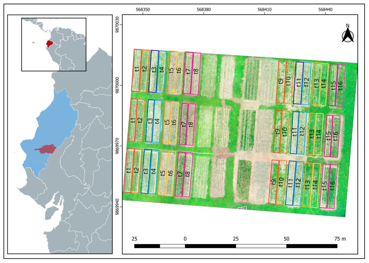
Figure 1. Location of the study area.: Manabí Province (left panel, light blue) and Santa Ana Canton (left panel, red) are shown, along with the experimental plots displaying their respective treatments (right panel). T1–T16 denote treatments and their replicates (Table A1, Appendix A). Different colors within the plots represent replicates of the same treatment.
Agriengineering 08 00177 g001
Figure 2. Photogrammetric processing workflow implemented in PIX4Dmapper.
Agriengineering 08 00177 g002
Figure 3. Orthomosaics obtained from the photogrammetric analysis of the two UAV flight missions. (A): Orthomosaic derived from the first flight mission conducted before crop sowing. (B): Orthomosaic derived from the flight mission conducted 89 days after sowing.
Agriengineering 08 00177 g003
Figure 4. Spectral indices with the highest predictive potential for edaphic properties and peanut crop morphological traits. (a,b) vNDVI (visible NDVI) orthomosaics derived from the flight conducted before sowing (a) and at 89 days after germination (b); (c,d) VIgreen (Vegetation Index Green) orthomosaics derived from the flights conducted before sowing (c) and at 89 days after germination (d); (e,f) RGBVI (Red–Green–Blue Vegetation Index) orthomosaics derived from the flights conducted before sowing (e) and at 89 days after germination (f); (g,h) HUE (Overall Hue Index) orthomosaics derived from the flights conducted before sowing (g) and at 89 days after germination (h); (i,j) RCC (Red Chromatic Coordinate Index) orthomosaics derived from the flights conducted before sowing (i) and at 89 days after germination (j).
Agriengineering 08 00177 g004
Figure 5. Heatmap of strong Spearman correlations (r ≥ 0.5) between edaphic properties and RGB-based spectral indices. γ = the real density; SBD = soil bulk density; Pr = porosity; θ F C = field capacity moisture conten; θ P W P = the permanent wilting point moisture content; GWC = Gravimetric Water Content; EC = Electrical Conductivity; N = total nitrogen; P = potassium; K = phosphorus; SOM = soil organic matter; WI = Woebbecke Index; ExB = Excess Blue; GR = Simple Red–Green Ratio; HUE = Overall Hue Index; PRI = Photochemical Reflectance Index; RCC = Red Chromatic Coordinate Index; vNDVI = visible NDVI; BI = Brightness Index; BGI = Simple Blue–Green Ratio/Blue–Green Pigment Index; TGI = Triangular Greenness Index; VEG = Vegetative Index; GLI = Green Leaf Index; MVARI = Modified Visible Atmospherically Resistant Vegetation Index; GCC = Green Percentage Index; RGBVI = Red–Green–Blue Vegetation Index; MGRVI = Modified Green–Red Vegetation Index; VIgreen = Vegetation Index Green; Red, Green, Blue = band reflectance values. More details in Table A3 (Appendix).
Agriengineering 08 00177 g005
Figure 6. Heatmap of strong Pearson correlations (r ≥ 0.5) between the traits and the RGB-based spectral indices. CL = chlorophyll; NW = nodule weight; vNDVI = visible NDVI; RGBVI = Red–Green–Blue Vegetation Index; VIgreen = Vegetation Index Green. See Table A4, Appendix for details.
Agriengineering 08 00177 g006
Table 1. RGB vegetation indices adapted from Biró et al., (2024) [30].
AcronymIndex NameEquation
WIWoebbecke Index G B R G
ExBExcess Blue 1.4 b g
GRSimple Red–Green Ratio G R
HUEOverall Hue Index a t a n ( 2 B G R 30.5 G R )
PRIPhotochemical Reflectance Index R G
RCCRed Chromatic Coordinate Index R R + G + B
vNDVIvisible NDVI 0.527 ( r 0.129       g 0.339   b 0.312 )
BIBrightness Index R 2 + B 2 + G 2 3 2
BGISimple Blue–Green Ratio; Blue–Green Pigment Index B G
TGITriangular Greenness Index G 0.39 R 0.61 B
VEGVegetative Index G R 0.667     B 0.334
GLIGreen Leaf Index 2 G R B 2 G + R + B
MVARIModified Visible Atmospherically Resistant Vegetation Index G B G + R B
GCCGreen Percentage Index G R + G + B
RGBVIRed–Green–Blue Vegetation Index G 2 B R G 2 + B R
MGRVIModified Green–Red Vegetation Ind G 2 R 2 G 2 + R 2
VIgreenVegetation Index Green G R G + R
Table 2. Parameters of stablished flights adapted from the DJI Phantom 4 Multispectral User Manual (2020).
ParameterDescription
Flight altitude55 m.a.s.l.
Flight speed6 m/s
Coverage area1 ha
Sensor type1” CMOS and 20 Mpx (RGB)
Lateral overlap70%
Frontal overlap80%
Flight time10h00 (for all flights)
Flight duration15 min
Table 3. Spearman correlation coefficient ranges [40,41].
GradeStrength of the Relationship
[0.00–0.20]No correlation
[0.20–0.35]Weak correlation
[0.35–0.50]Moderate correlation
[0.50–1.00]Strong correlation
Table 4. Predictive models using Random Forest and k-Nearest Neighbors between soil properties and spectral indices. SBD: soil bulk density; SOM: soil organic matter; R2: coefficient of determination; MSE: mean squared error; MAE: mean absolute error; OHI: Overall Hue Index; RCC: Red Chromatic Coordinate Index; vNDVI: visible Normalized Difference Vegetation Index; RGBVI: Red–Green–Blue Vegetation Index.
IndexRandom Forestk-Nearest Neighbors
R2MSEMAER2MSEMAE
SBD
RGBVI0.5820.474.200.030.020.13
vNDVI0.7014.373.510.090.030.14
SOM
HUE0.620.110.270.060.280.53
RCC0.870.040.180.130.250.49
Table 5. Predictive models using the Random Forest algorithm. Chlorophyll: chlorophyll content; Nodulation: nodule weight; R2: coefficient of determination; MSE: mean squared error; MAE: mean absolute error; vNDVI: visible Normalized Difference Vegetation Index; RGBVI: Red–Green–Blue Vegetation Index; VIgreen: Vegetation Index Green.
IndexChlorophyllNodulation
R2MSEMAER2MSEMAE
RGBVI0.120.020.120.130.040.17
vNDVI0.510.010.090.160.040.17
HUE0.7313.23.180.390.030.15
RCC---0.340.030.16
Table 6. Regression results obtained with the k-Nearest Neighbors algorithm. Chlorophyll: chlorophyll content; Nodulation: nodule weight; R2: coefficient of determination; MSE: mean squared error; MAE: mean absolute error; vNDVI: visible Normalized Difference Vegetation Index; RGBVI: Red–Green–Blue Vegetation Index; VIgreen: Vegetation Index Green.
IndexChlorophyllNodulation
R2MSEMAER2MSEMAE
RGBVI0.4526.634.990.180.040.14
vNDVI0.4625.594.950.250.040.15
HUE0.4725.384.560.270.040.14
RCC---0.310.040.14
Disclaimer/Publisher’s Note: The statements, opinions and data contained in all publications are solely those of the individual author(s) and contributor(s) and not of MDPI and/or the editor(s). MDPI and/or the editor(s) disclaim responsibility for any injury to people or property resulting from any ideas, methods, instructions or products referred to in the content.