Deep Learning for Semantic Segmentation in Crops: Generalization from Opuntia spp.

Abstract

Semantic segmentation of UAV–acquired RGB orthomosaics is a key component for quantifying vegetation cover and monitoring phenology in precision agriculture. This study evaluates a representative set of CNN–based architectures (U–Net, U–Net Xception–Style, SegNet, DeepLabV3+) and Transformer–based models (Swin–UNet/Swin–Transformer, SegFormer, and Mask2Former) under a unified and reproducible protocol. We propose a transfer–and–consolidation workflow whose performance is assessed not only through region–overlap and pixel–wise discrepancy metrics, but also via boundary–sensitive criteria that are explicitly linked to orthomosaic–scale vegetation–cover estimation by pixel counting under GSD (Ground Sample Distance) control. The experimental design considers a transfer scenario between morphologically related crops: initial training on Opuntia spp. (prickly pear), direct (“zero–shot”) inference on Agave salmiana, fine–tuning using only 6.84% of the agave tessellated set as limited target–domain supervision, and a subsequent consolidation stage to obtain a multi–species model. The evaluation integrates IoU, Dice, RMSE, pixel accuracy, and computational cost (time per image), and additionally reports the BF score and HD95 to characterize contour fidelity, which is critical when area is derived from orthomosaic–scale masks. Results show that Transformer-based approaches tend to provide higher stability and improved boundary delineation on Opuntia spp., whereas transfer to Agave salmiana exhibits selective degradation that is mitigated through low–annotation–cost fine-tuning. On Opuntia spp., Mask2Former achieves the best test performance (IoU 0.897 +/− 0.094; RMSE 0.146 +/− 0.002) and, after consolidation, sustains the highest overlap on both crops (IoU 0.894 +/− 0.004 on Opuntia and IoU 0.760 +/− 0.046 on Agave), while preserving high contour fidelity (BF score 0.962 +/− 0.102/0.877 +/− 0.153; HD95 2.189 +/− 3.447 px/8.458 +/− 16.667 px for Opuntia/Agave), supporting its use for final vegetation–cover quantification. Overall, the study provides practical guidelines for architecture selection under hardware constraints, a reproducible transfer protocol, and an orthomosaic–oriented implementation that facilitates integration into agronomic and remote–sensing workflows.

1. Introduction

The digital transformation of agriculture seeks to optimize production by integrating advanced technologies in crop management. The United Nations Sustainable Development Goals (SDGs), particularly SDG 2 (Zero Hunger), underscore the need for sustainable and efficient agricultural practices to ensure food security [1]. Precision agriculture (PA) has become a promising approach for increasing the efficiency and sustainability of crops through site–specific management, cost reduction and input minimization [2].

Based on observation and site–specific action, PA relies on remote sensing platforms such as satellites, manned aircraft, and unmanned aerial vehicles (UAVs) that allow the condition of the vegetation in each plot to be quantified at high resolution [3]. In particular, drones have become widespread due to their flexibility, low operating cost, and high spatial resolution, facilitating detailed monitoring of indicators such as vigor, water content, and plant density [4,5].

Previous studies have demonstrated the value of integrating UAV images with computer vision techniques to map crop health at different phenological stages [6], which has enabled new opportunities to estimate leaf areas, detect water stress, pests, or diseases, and even predict yields with greater timeliness and precision than traditional methods [7]. The current challenge is to develop general, robust image analysis algorithms for multiple crop types to scale PA beyond species-specific solutions.

In this context, Mexico has emblematic crops whose management systems could benefit from automated multi–crop monitoring. One of them is the prickly pear (Opuntia spp.), a perennial cactus of food and industrial importance. In 2022, about 12,491 ha of prickly pear were cultivated, with a production of 872 kt and a value of 2981 M MXN; 7.4% of that production was exported, reflecting its economic relevance [8,9]. This crop stands out for its resistance to arid conditions and its versatility in uses (vegetable, forage, cosmetics, bioenergy), being a traditional component of Mexican agriculture [10]. Additionally, in states such as Hidalgo, prickly pear coexists with other semi–arid crops of value, such as the pulque agave (Agave salmiana), used to produce aguamiel and pulque. Hidalgo is the principal national producer of pulque agave (5079 ha) and ranks among the top producers of prickly pear fruit and tuna fruit [11]. Due to its climatic adaptation, Opuntia is regarded as a resilient crop under water-stress scenarios associated with climate change; however, maximizing sustainable productivity requires precise and repeatable plot-scale monitoring [12].

In UAV RGB orthomosaics, Opuntia and Agave share semi-arid imaging conditions (exposed soil, pronounced shadows, textured and heterogeneous backgrounds), yet they differ in plant geometry (cladodes vs. rosettes), occlusion patterns, and boundary characteristics; this combination defines a demanding setting to evaluate cross-domain transfer. The agronomic and socioeconomic relevance of both species is widely documented, both for their role in productive diversification in arid regions and for the associated value chains in food, fiber, and bioenergy [13,14].

Despite advances in agricultural computer vision, a significant gap persists: most segmentation models trained for a specific crop or condition tend to degrade their performance when applied to different scenarios without recalibration [15,16]. In general, this is due to variations among crops (morphology, color, texture) and among fields (lighting, background, phenology) that alter the pixel distribution in the images. Traditional CNN–based algorithms efficiently learn features from the training set but tend to overfit; as a consequence, their generalization ability is limited. This need to re–label data for each new situation constitutes a bottleneck for practical applications. Various authors have emphasized that the scarcity of annotated data and the intrinsic variability of agricultural conditions make it difficult to create universal segmenters [17]. Operationally, out-of-domain degradation typically manifests as vegetation fragmentation, confusion with soil/shadows, and loss of contour continuity, which limits model reuse across fields and species without intensive retraining. Moreover, due to the common class imbalance between vegetation and soil, global metrics can artificially inflate the apparent model quality; therefore, the evaluation is grounded on overlap measures and boundary-sensitive criteria (Dice/F1, BF score, and HD95), which jointly quantify spatial agreement and geometric boundary deviation relative to the manual references. Under this definition, “stability” denotes lower sensitivity of the segmenter to variations in illumination, background, and morphology (i.e., reduced degradation under domain shift), whereas “boundary delineation” denotes higher geometric fidelity of contours (higher BF score and lower HD95).

In the case of prickly pear, until recently, there were virtually no publicly available datasets or research dedicated to its automatic segmentation. An initial advance was the work of Duarte–Rangel et al., who binarily segmented vegetation of Opuntia spp. in UAV orthomosaics using U–Net, DeepLabV3+, and U–Net Xception, achieving IoU values of 0.66–0.67 to identify the vegetation area [18]. In parallel, Gutiérrez–Lazcano et al. demonstrated the usefulness of a U–Net Xception–Style model to detect the weed Cuscuta spp. in RGB orthomosaics captured with UAV [19]. However, both studies are limited to CNN–based architectures and do not address knowledge transfer to other crops, leaving open the need to explore approaches with greater generalization capacity. Patch-based processing facilitates training on large orthomosaics while preserving local detail (boundaries and soil–vegetation transitions). In contrast, orthomosaic–scale inference and reconstruction recover spatial continuity in the final output.

On the other hand, Vision Transformers have revolutionized general computer vision by modeling global dependencies through self–attention [20]. In principle, this ability to capture context could lead to more robust segmentation under spatial and textural variations. Recent agricultural studies report competitive results for weed and crop segmentation with Transformer or hybrid CNN–Transformer designs [21,22,23]. Therefore, the balance between CNN/Transformer architectures in agriculture, and their ability to transfer knowledge with minimal recalibration, remains an open questions that motivate the present study. Recent agricultural literature supports the potential of self-attention for crop/weed segmentation with SegFormer-like models, as well as for multi-source integration schemes that combine remote-sensing observations with meteorological variables, and even for spectral–spatial attention designs; collectively, these results suggest that Transformers can provide stronger contextual robustness under typical field variability [24,25,26]. However, for the comparison to be methodologically sound and actionable for adoption, it is also necessary to account for data requirements, memory footprint, and sensitivity to image resolution and partitioning, as these factors directly determine operational feasibility. In this study, hardware constraints are primarily framed in terms of GPU memory, training and inference time, and deployment feasibility within precision-agriculture workflows under limited computational resources.

This study focuses on quantifying, under a unified experimental framework, the generalization and transfer capability of CNN- and Transformer-based architectures between Opuntia spp. and Agave salmiana, and on developing and validating a consolidated multi-species model that simultaneously preserves accuracy and boundary fidelity with minimal recalibration. To foster adoption and reproducibility, we release the annotated dataset, code, and experimental artifacts (including hyperparameter tables and configuration details), and we formalize an evaluation cycle to reduce the need for re-labeling when transferring models across species and field scenarios. To support these goals with comparable evidence, we jointly report overlap metrics, boundary-sensitive criteria, and computational-efficiency measures.

The following sections describe the study area and the capture of RGB orthomosaics using a UAV; the dataset and its pixel-level annotation; and the unified experimental framework (architectures and metrics). They also formalize the multicrop evaluation cycle, present an orthomosaic-scale pipeline with leaf area quantification, report a precision–efficiency benchmark, document reproducibility artifacts, and conclude with adoption guidelines.

2. Materials and Methods

2.1. Study Area

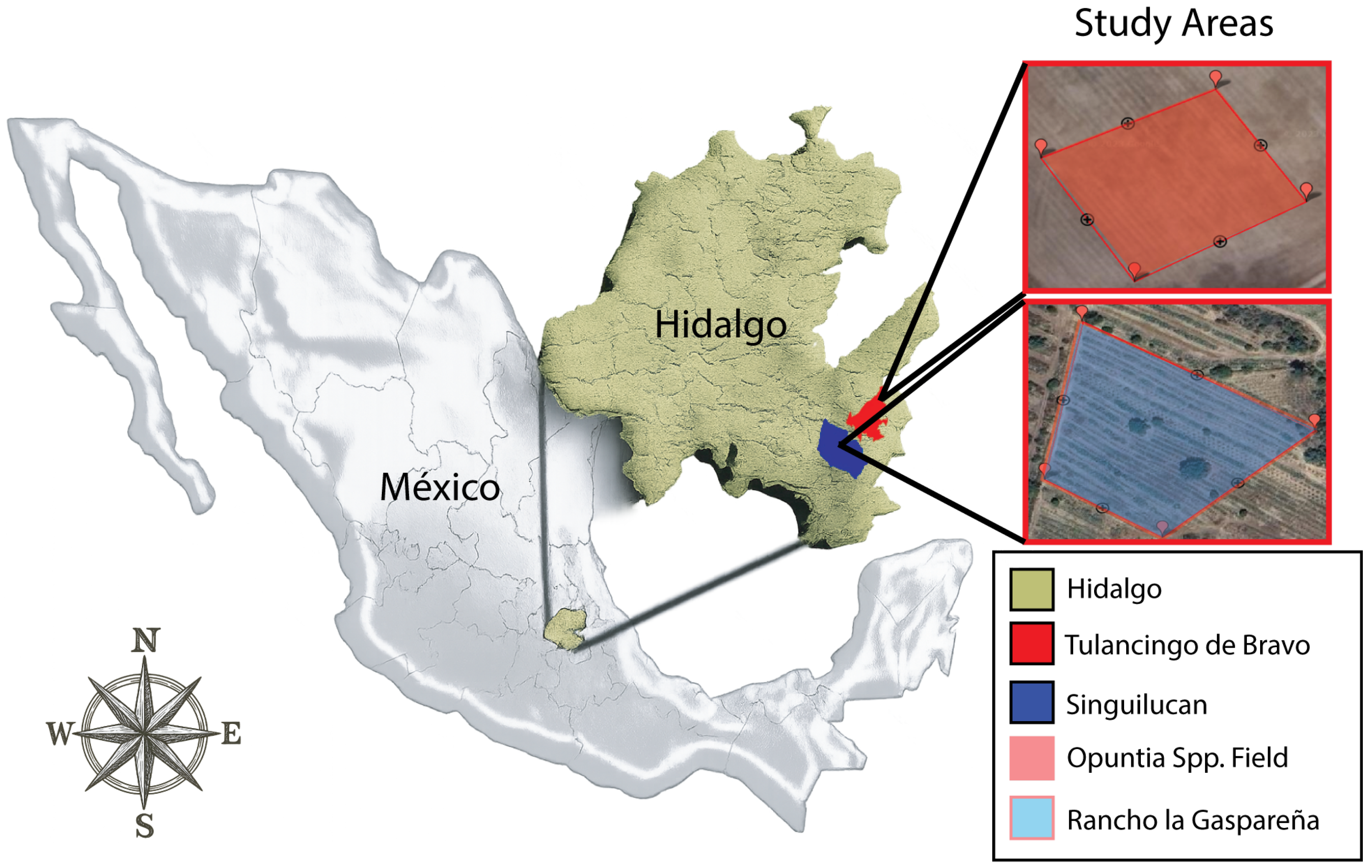
2.1.1. Study Area A—Opuntia spp., Tulancingo

The study area corresponds to an experimental prickly pear (Opuntia spp.) plot located in the Tulancingo Valley, Hidalgo, Mexico, georeferenced at $20.{12555}^{\circ }\mathrm{N}$ and $-98.{37867}^{\circ }\mathrm{W}$, a short distance from the Universidad Politécnica de Tulancingo (Figure 1). The unit was delimited at approximately $539{\mathrm{m}}^2$ to have a representative sample that allows an assessment of the acquisition and processing stages at the orthomosaic scale; the site selection obeys criteria of accessibility and proximity that optimize field logistics and the detailed characterization of agroecosystem components.

2.1.2. Study Area B—Agave salmiana, Rancho La Gaspareña, Singuilucan

The second experimental site is located at Rancho La Gaspareña, at geographic coordinates $19.{9692}^{\circ }$ latitude and $-98.{5052}^{\circ }$ longitude, in the community of Tlacoticpa, municipality of Singuilucan, Hidalgo, Mexico. The ranch is located at an average altitude of $2490\mathrm{m}\mathrm{a}.\mathrm{s}.\mathrm{l}.$ on the eastern slope of the Sierra de Pachuca (Figure 1) and maintains approximately $15\mathrm{ha}$ of Agave salmiana (varieties “manso” and “chalqueño”) under rainfed conditions [27,28].

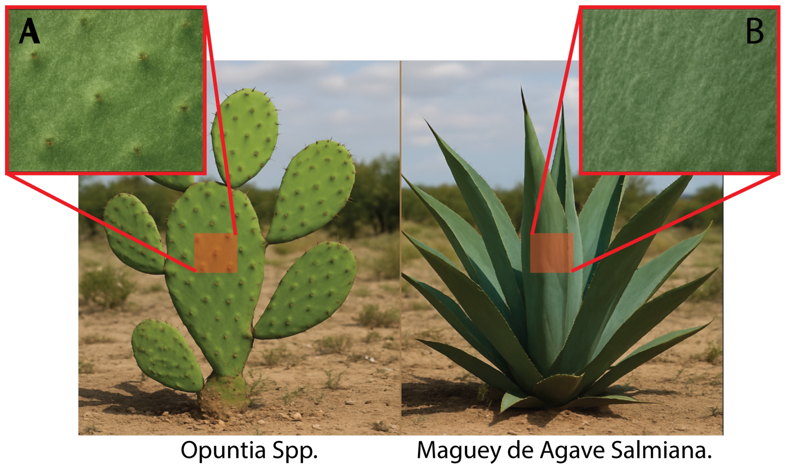
The radial arrangement of agave leaves provides an ideal setting for evaluating the transferability of segmentation models. Unlike the flat pads of Opuntia spp., agave exhibits more complex textural and geometric signatures, such as concentric patterns, cross shadows, and chromatic variations. These morphological differences, rather than being an obstacle, confer shape-, color-, and texture-based features that reinforce the model’s robustness, as shown in Figure 2. For this reason, Rancho La Gaspareña represents an ideal case to test the capacity for cross–crop generalization, allowing us to assess how much of the representation learned in prickly pear is preserved when facing succulents with a different habit under equivalent climatic and edaphic conditions.

2.2. Data Acquisition

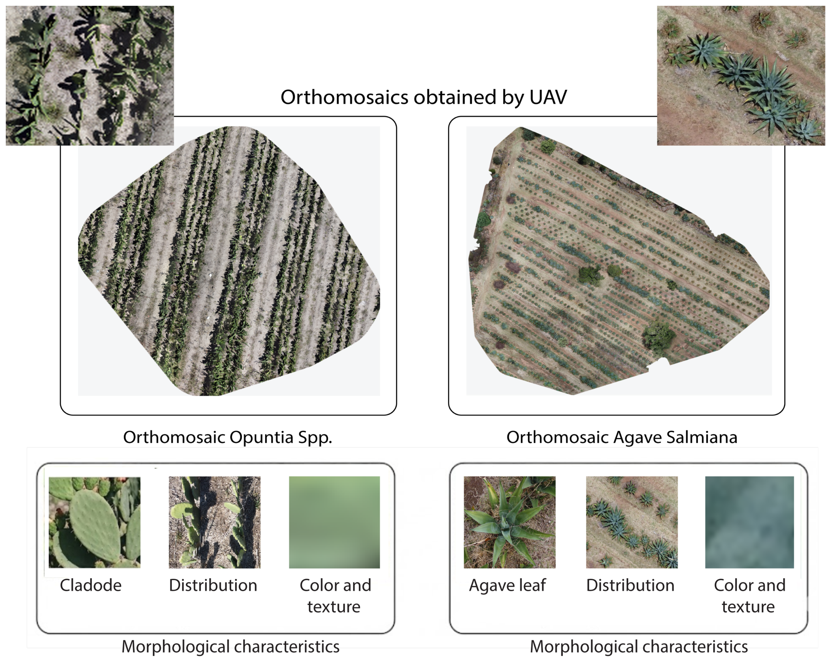
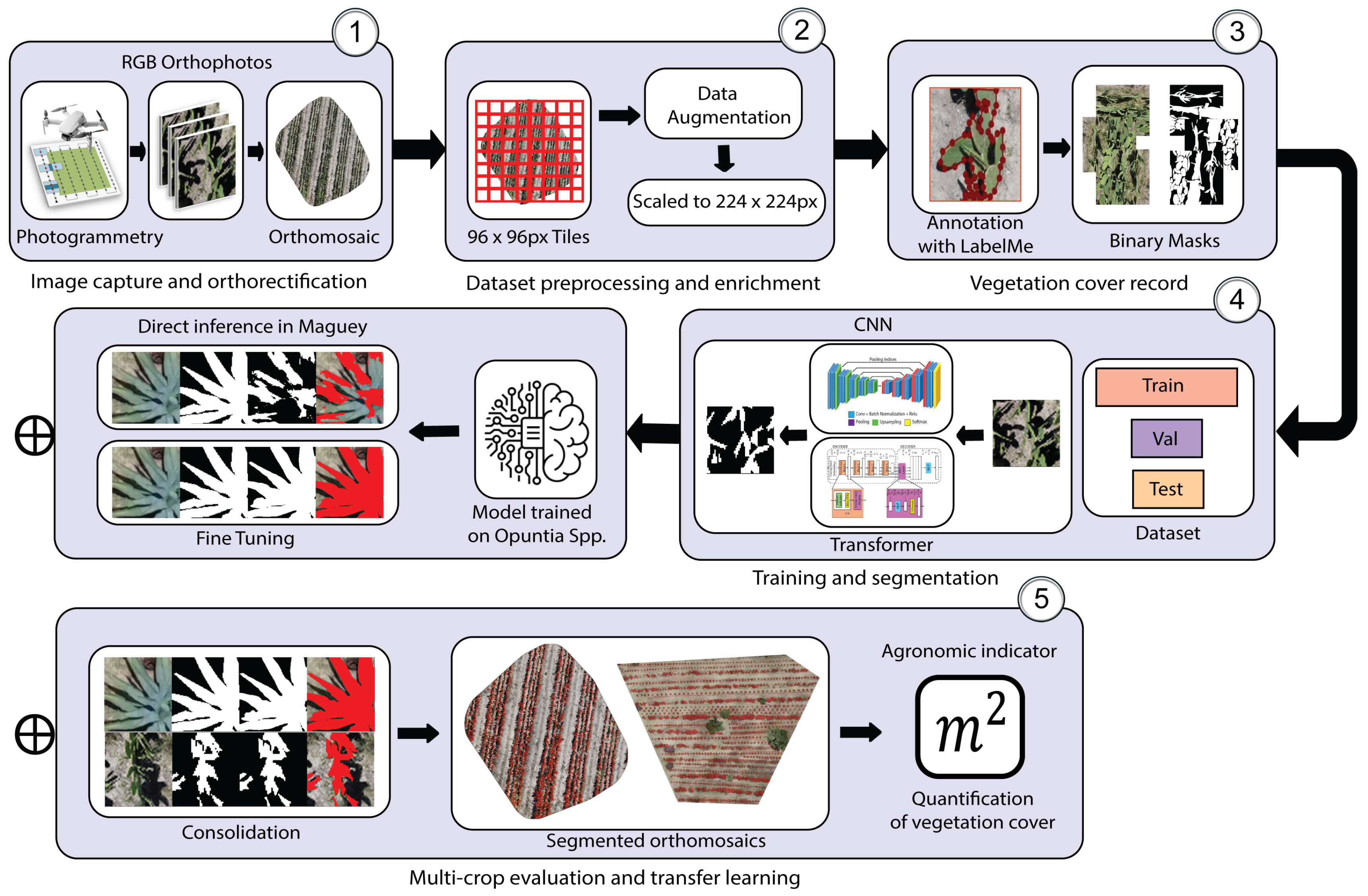
The orthomosaic of Opuntia spp. was obtained using a DJI Mavic 2 Mini (DJI, Shenzhen, China) by planning the mission in Dronelink (Dronelink, Austin, TX, USA) at a height of 4 m. The flight plan combined three camera orientations and ensured 75% forward overlap and 70% lateral overlap, generating 443 RGB photographs at a resolution of 12 MP. Processing in WebODM (v2.8.4) yielded an average GSD (Ground Sample Distance) of 1.02 cm per pixel, corresponding to approximately 72 image pixels per cladode within the orthomosaic.

To compare with Agave salmiana and match the information density achieved in the prickly pear orthomosaic of an average of 72 pixels per cladode, the flight height was calculated from the linear relationship between ground distance and pixel size: since each agave leaf covers an area about six times larger, 61 m reproduces, on average, the number of pixels per leaf organ. This adjustment standardizes the geometric scale between crops, reduces the number of images, and shortens processing time without compromising the definition of contours and textures.

The mission was conducted at 11:00 h, replicating the prickly pear study’s solar window to ensure uniform illumination, minimize shadows, and maintain radiometric coherence across images. With 85% forward overlap and 80% lateral overlap, the flight covered 1 km, captured 75 RGB photographs at 12 MP, and generated an orthomosaic with an average GSD of 1.8 cm/pixel, enabling comparison of the morphological patterns of both succulent species without scale-related bias. The two orthomosaics obtained are shown in Figure 3.

2.3. Dataset

Two independent datasets were constructed from the RGB orthomosaics of Opuntia spp. and Agave salmiana. Details of each set are shown in

Table 1. Comparative characteristics of the datasets used for segmenting Opuntia spp. and Agave salmiana.

Characteristic	Opuntia spp.	Agave salmiana
Original crops	186	335
Data augmentation	Horizontal/Vertical flips and rotations $\pm {90}^{\circ }/{180}^{\circ }$	Not applied
Total images after augmentation	549	335
Train/test/val split	411/83/55	234/68/33
Purpose	Training from scratch	Fine–tuning the model

. In both cases, black padding was first applied so that the dimensions were exact multiples and non–overlapping crops of $96\times 96$ pixels were extracted. These were manually annotated with Labelme to generate binary masks. The $96\times 96$ px tiling size was selected as a compromise between sufficient local context and computational efficiency: at the acquisition resolutions (GSD ≈ 1.02 cm/px for Opuntia and 1.8 cm/px for Agave), each crop covers approximately ~0.98 m and ~1.73 m per side, respectively, which preserves soil–vegetation transitions, shadows, and boundary fragments that are informative for binary segmentation. This choice is consistent with prior patch-based segmentation practices on UAV RGB orthomosaics, where crops of this order have been reported to retain discriminative information for vegetation delineation [19]. To mitigate the loss of orthomosaic-scale context, the methodological scheme operates through tiling: inference is performed per tile and predictions are reassembled into the original orthomosaic geometry, so the spatial continuity of the final product is recovered during reconstruction.

Augmentation was applied only to the Opuntia base set to increase apparent variability in the smaller dataset, whereas Agave was kept non-augmented to preserve its distribution as the target adaptation domain under limited labeling. Validation and test splits for both crops were kept non-augmented, and results are reported by phase (base training, direct inference, and consolidation) to enable cross-domain comparisons on non-augmented data.

The RGB crops and their masks were rescaled to $224\times 224$ pixels, as this is the reference resolution used during the pretraining of most ImageNet–based backbones; maintaining this format avoids reconfiguring input layers and allows leveraging robust initial weights, reducing convergence time and the risk of overfitting. Rescaling was implemented using bilinear interpolation for RGB images and nearest-neighbor interpolation for binary masks to preserve discrete labels and avoid class-mixing artifacts along boundaries. It also increases the relative prominence of leaf edges and textures, thereby improving the network’s ability to discriminate contours accurately.

Black padding was used exclusively to enforce orthomosaic dimensions as exact multiples of the cropping window and to enable regular tiling. For the masks, padded regions were consistently treated as background. To prevent bias or artifacts, tiles whose area originates from padding were excluded from the annotated training/evaluation set, and all metrics were computed only over valid (non-padded) orthomosaic regions. The datasets are publicly available in the repository https://github.com/ArturoDuarteR/Semantic-Segmentation-in-Orthomosaics.git (accessed on 20 November 2025).

2.4. Semantic Segmentation Techniques

Semantic segmentation assigns a class to each pixel, producing label maps that separate regions of interest from the background. In precision agriculture, it enables the automated delineation of cultivated areas and target plants in UAV imagery. Its deployment is challenged by strong field variability (illumination changes, phenological stages, weeds) that can reduce robustness [15], as well as the high spatial resolution of UAV data, which increases training and inference costs.

Deep learning has become the dominant approach for vegetation segmentation. Fully Convolutional Networks (FCN) enabled end–to–end learning for dense prediction [29], and encoder–decoder designs such as U–Net and SegNet improved spatial delineation. U–Net uses skip connections to fuse encoder and decoder features and performs well even with limited data [30], whereas SegNet reuses pooling indices for a more memory–efficient decoder [31]. DeepLabV3+ further strengthened multiscale representation through atrous convolutions and ASPP, coupled with a lightweight decoder to refine boundaries [32]. Efficiency–oriented variants such as U–Net Style Xception replace the encoder with depthwise–separable blocks, often improving Dice/IoU in heterogeneous UAV agricultural scenes [33].

Transformer–based segmentation models incorporate attention to capture long–range dependencies, but early ViT formulations are computationally expensive due to global attention over image patches [34]. More efficient hierarchical alternatives include Swin Transformer (shifted windows) [35], SegFormer (efficient backbone with a lightweight MLP decoder) [23], and Mask2Former, which predicts masks via queries in an attention–based decoder and unifies multiple segmentation paradigms [36].

Based on this landscape, seven representative architectures were selected for comparison: U–Net, DeepLabV3+, U–Net Style Xception, SegNet, Swin-Transformer, SegFormer, and Mask2Former.

2.4.1. UNet

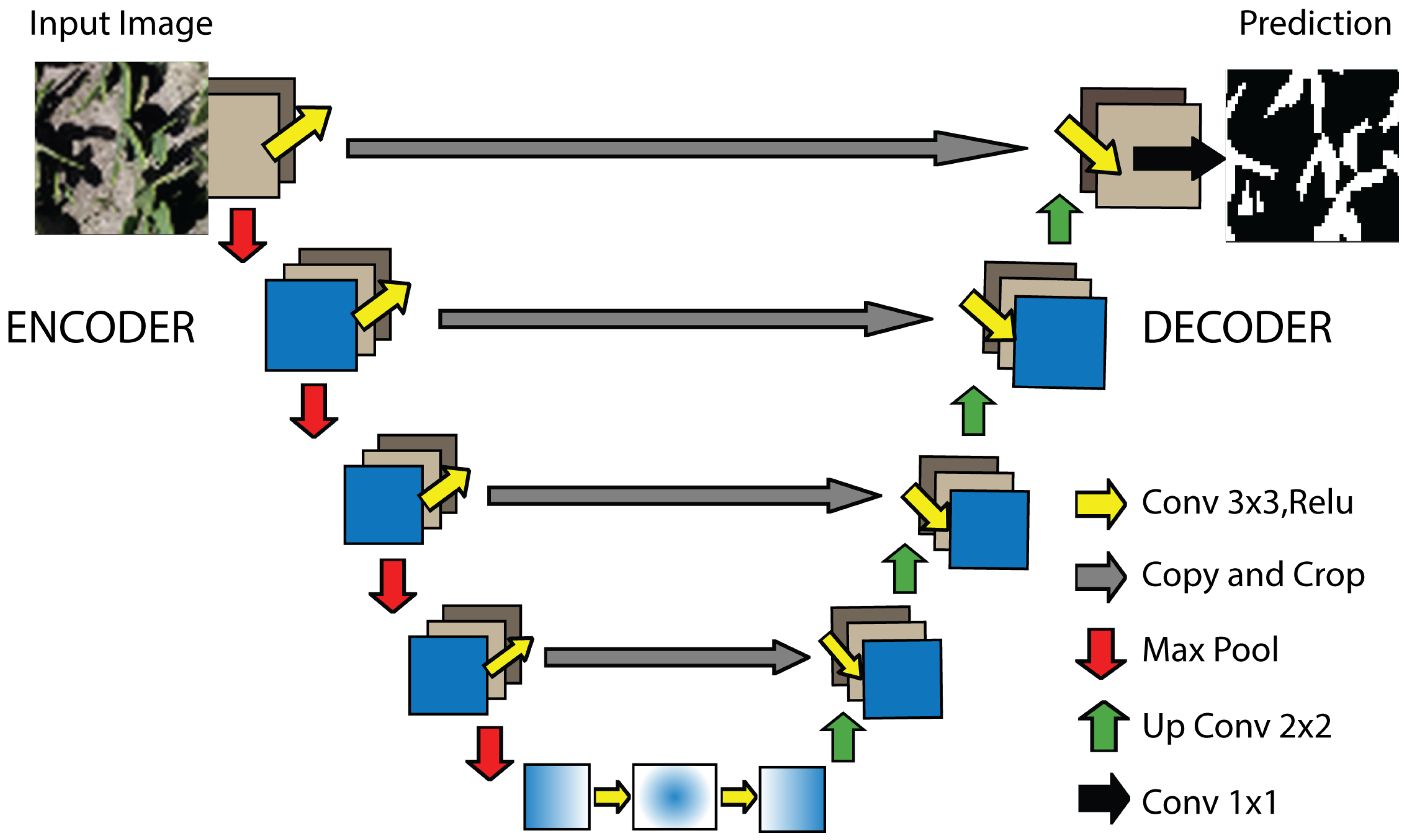
UNet adopts a U-shaped architecture composed of a symmetric encoder–decoder pair connected through a central bottleneck. Its defining element is the set of skip connections between homologous stages, which preserves fine-grained spatial details and fuses them with higher-level semantic representations, enabling accurate pixel-wise segmentation even with limited training data (Figure 4). In the encoder, each stage applies two $3\times 3$ convolutions with ReLU activation, followed by max-pooling to reduce spatial resolution while increasing the number of feature channels; the decoder reverses this process via transposed convolutions and feature fusion with the corresponding skip–connections. This hierarchical design captures both contextual information and local boundaries without dense layers that would inflate the parameter count; consequently, UNet remains memory-efficient, end-to-end trainable, and less prone to overfitting when combined with intensive data augmentation [30].

2.4.2. DeepLabV3+

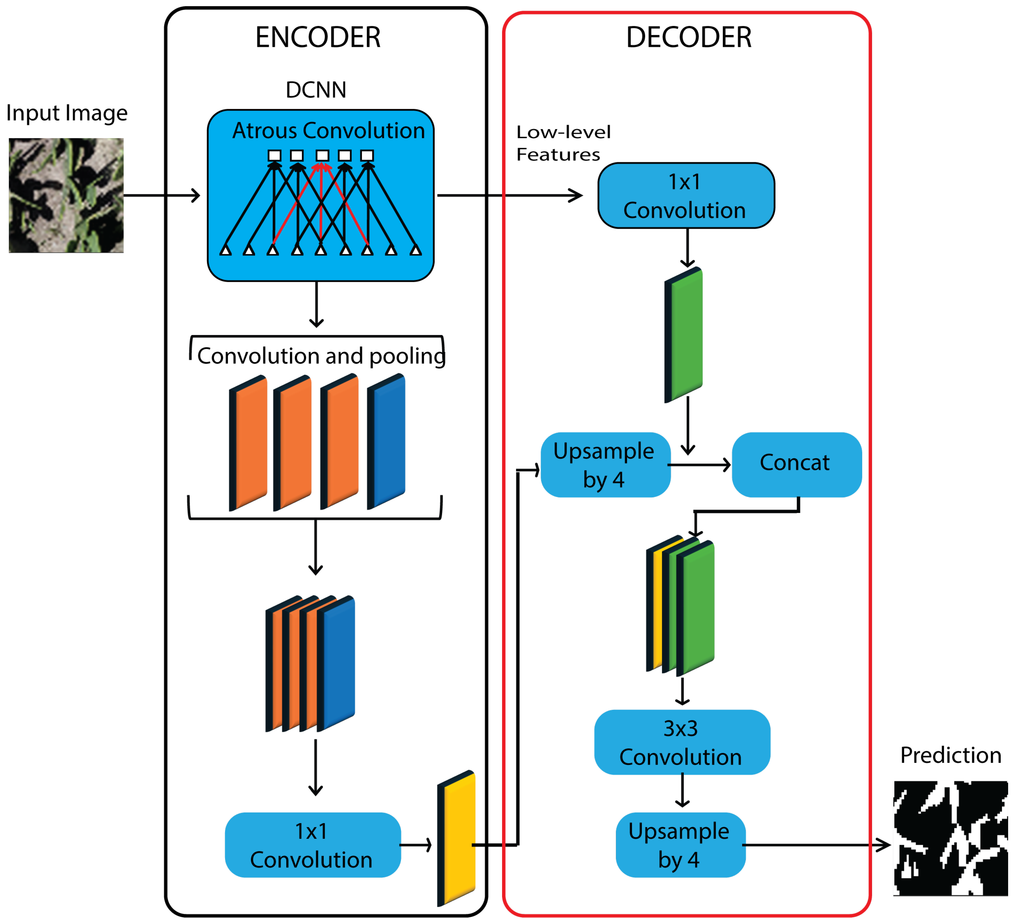
DeepLabV3+ (Figure 5) is an encoder–decoder semantic segmentation architecture that couples atrous (dilated) convolutions with an Atrous Spatial Pyramid Pooling (ASPP) module to aggregate multi-scale context by sampling feature maps at multiple dilation rates while preserving spatial resolution; the encoder is commonly instantiated with an Xception backbone based on depth-wise separable convolutions to reduce parameters and computation without sacrificing representational power, and a lightweight decoder then upsamples the ASPP output and fuses it with low-level encoder features to restore fine spatial detail, yielding sharper boundary localization and improved delineation of irregular objects with marginal additional overhead, while remaining modular with respect to alternative backbones for accuracy–efficiency trade-offs [32].

2.4.3. UNet Style Xception

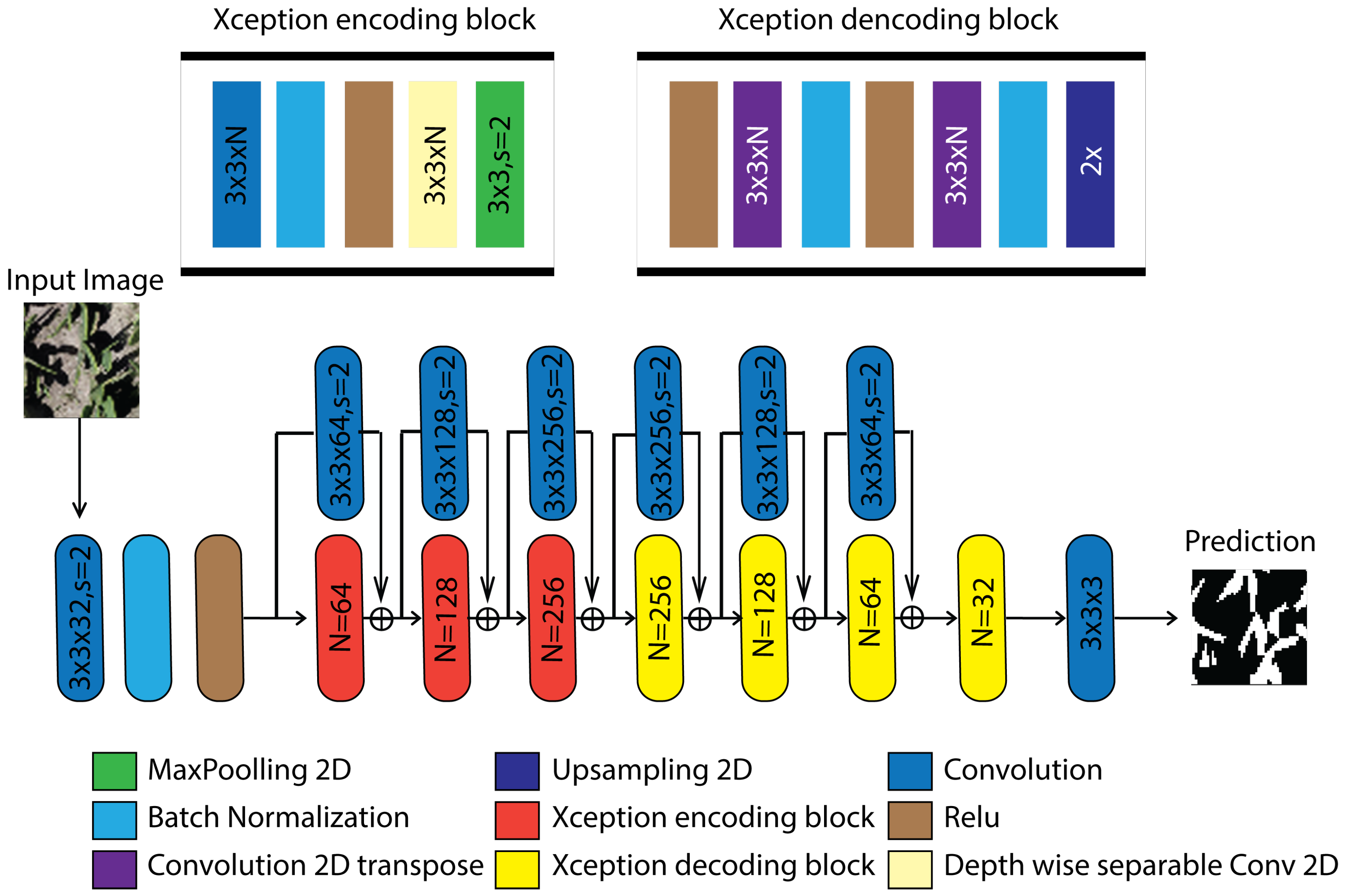
UNet Style Xception (Figure 6) preserves the UNet encoder–decoder topology with skip connections while replacing the conventional encoder with Xception entry/middle/exit flows based on depth-wise separable convolutions and internal residual shortcuts, thereby reducing parameterization and improving semantic feature extraction; in this configuration, standard convolutional blocks are reformulated as depthwise–pointwise sequences that enhance gradient propagation and accelerate convergence, and the resulting latent representation can be complemented by a compact context module (e.g., reduced ASPP or channel–pixel attention) to expand the receptive field without degrading spatial resolution, after which the decoder upsamples and concatenates low-level features to recover acceptable boundaries through additional separable convolutions, achieving improved pixel-wise delineation at lower computational cost, consistent with the Dice gains reported by Moodi et al. [37].

2.4.4. SegNet

SegNet is a fully convolutional encoder–decoder architecture in which the encoder follows the VGG–16 convolutional stages with ReLU activations and max-pooling, while the decoder performs non-linear upsampling by unpooling using the stored max-pooling indices, thereby reconstructing sparse high-resolution feature maps without learning deconvolution kernels (Figure 7). Each unpooling step is followed by convolutional refinement to recover spatial structure, progressively restoring the original resolution, and the network terminates with a pixel-wise classifier (e.g., binary or multi-class) applied to the restored feature maps. By reusing pooling switches, SegNet reduces memory footprint and computational overhead relative to decoders that require learned upsampling, while maintaining competitive boundary localization through index-guided spatial reconstruction [31].

2.4.5. Swin–Transformer

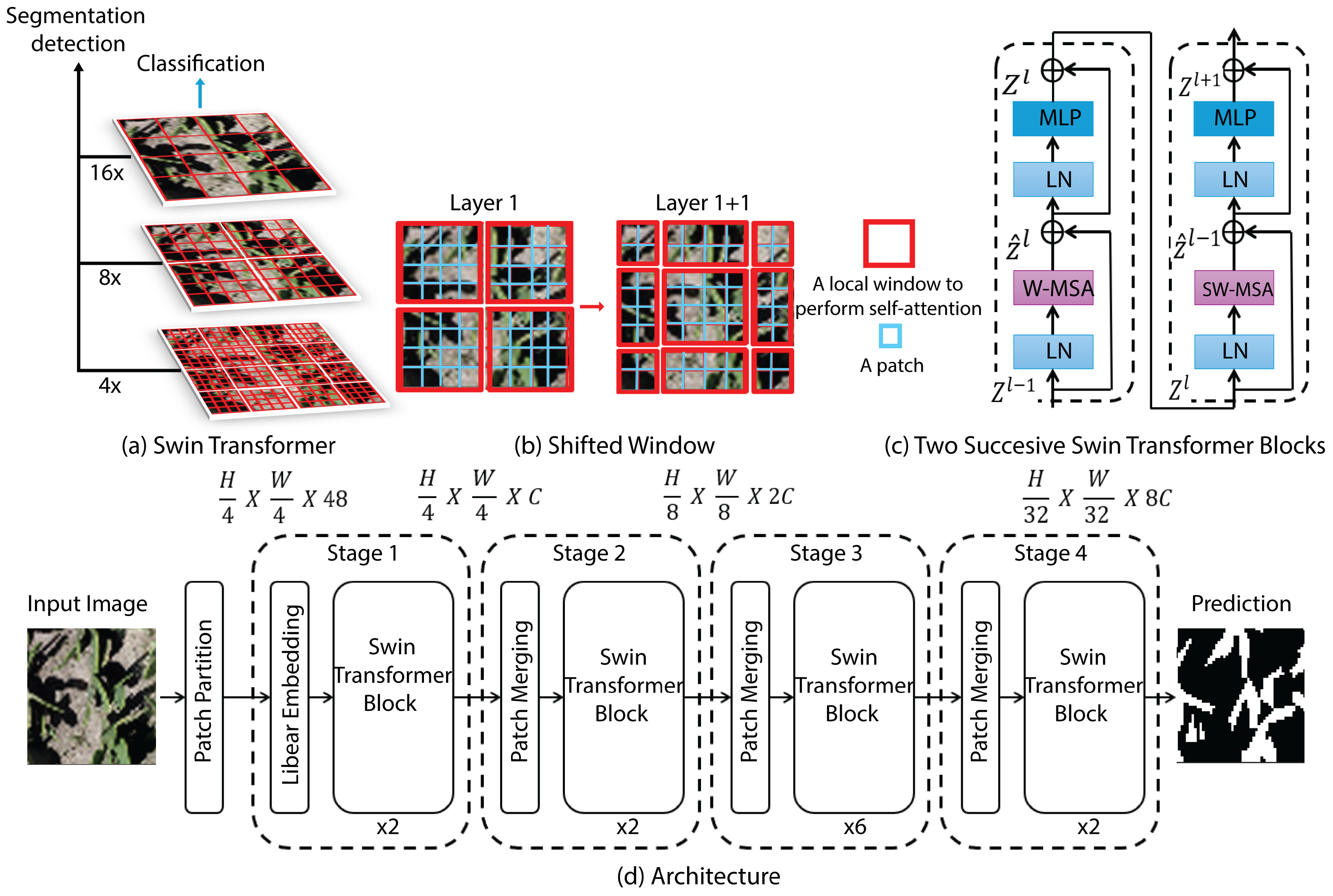
Swin–Transformer is a hierarchical vision Transformer that constructs multi-scale feature representations via window-based self-attention, enabling efficient modeling of spatial dependencies in scenes with substantial scale variability. Self-attention is computed within non-overlapping local windows to control complexity, while the shifted-window scheme alternates the window partitioning across consecutive layers to promote cross-window information exchange and approximate global context without the quadratic cost of dense attention. The backbone is organized into four pyramid stages: the image is first embedded into fixed-size patch tokens; successive Swin blocks perform intra-window attention; and patch-merging operations downsample the spatial grid while increasing the channel dimensionality, yielding progressively more abstract features (Figure 8). For semantic segmentation, this backbone is typically integrated into an encoder–decoder design in which the encoder supplies multi-resolution representations and a symmetric decoder performs patch-expanding upsampling and fuses corresponding stages through skip connections (UNet-like) to restore full resolution and produce dense pixel-wise predictions [35].

2.4.6. SegFormer

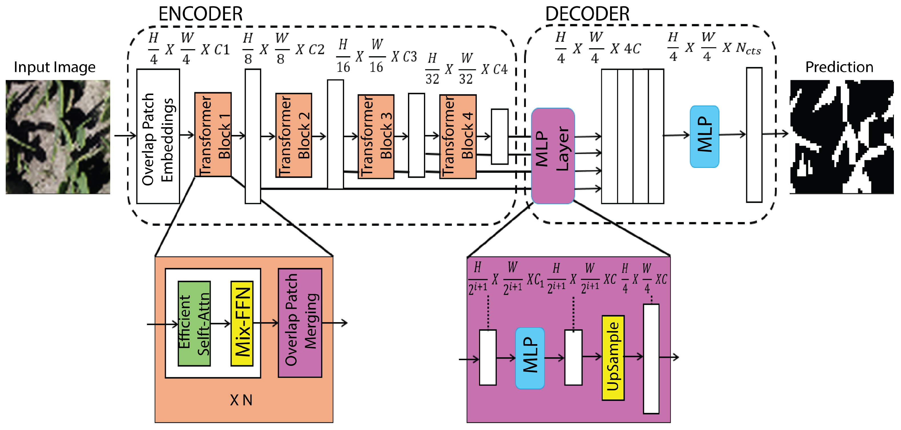
SegFormer is an efficient Transformer-based semantic segmentation architecture that couples a hierarchical Mix Transformer (MiT) encoder with a lightweight all-MLP decoder to achieve strong accuracy under constrained computation. The MiT backbone produces multi-scale feature maps via stage-wise token representations and efficient self-attention mechanisms that capture long-range dependencies without the prohibitive cost of early ViT designs, while normalization and pointwise ($1\times 1$) projections facilitate stable feature mixing across channels. Instead of employing computationally intensive context modules (e.g., ASPP) or heavy convolutional decoders, SegFormer uses linear projections to align channel dimensions and fuses the multi-resolution features with minimal overhead, yielding a compact segmentation head that is memory-efficient and fast at inference (Figure 9). This encoder–decoder formulation provides a favorable accuracy–efficiency trade-off for high-resolution semantic segmentation where throughput and resource usage are critical [23].

2.4.7. Mask2Former

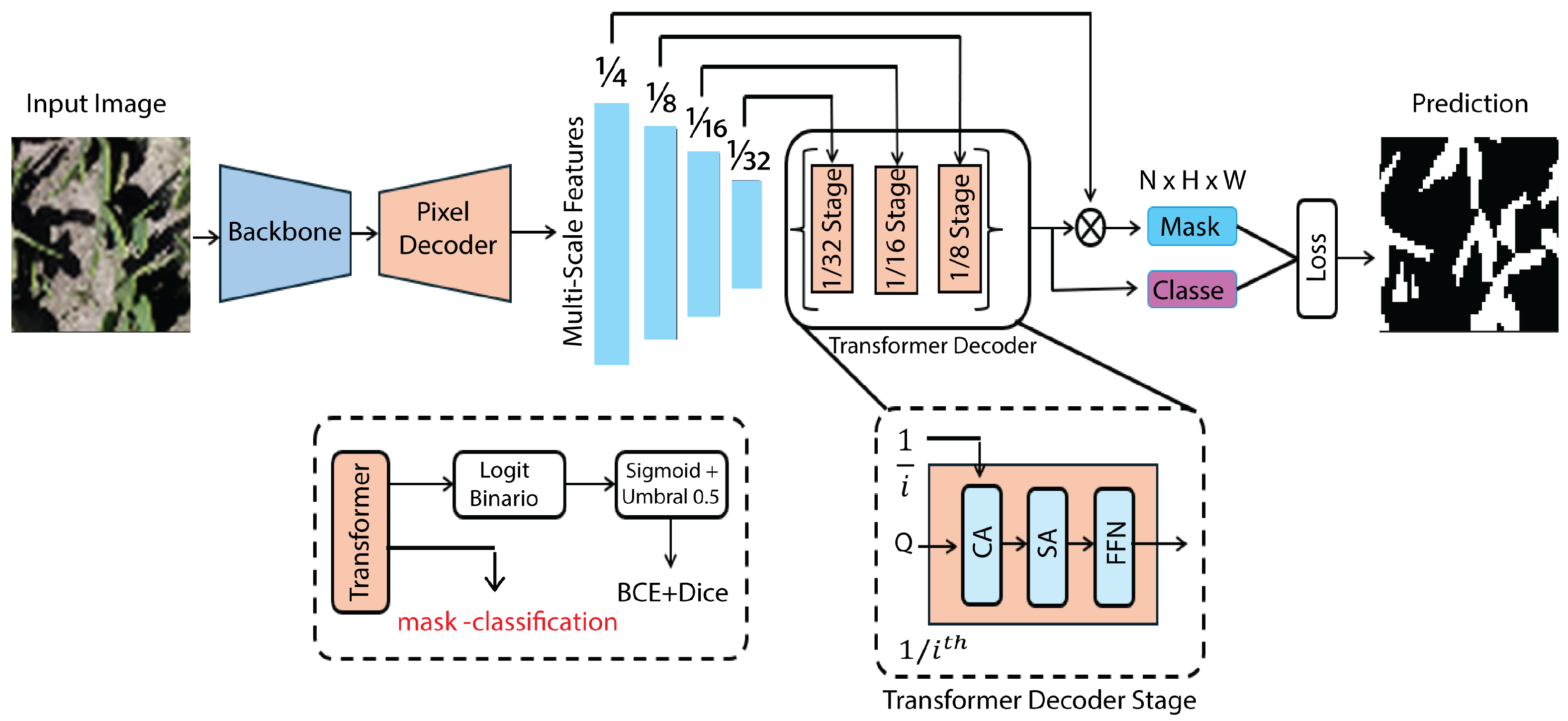
Mask2Former formulates segmentation as a set prediction problem in which a fixed number of learnable queries jointly infer class labels and dense masks, enabling a single architecture to support semantic, instance, and panoptic outputs. Its central contribution is masked cross-attention: at each decoder layer, the attention logits between queries and spatial tokens are multiplicatively gated by a query-specific binary/soft mask, restricting information flow to the predicted region and enforcing region-conditioned feature aggregation. This coupling reduces spurious context mixing, strengthens the separation of disconnected regions, and yields sharper boundary localization than unconstrained global attention decoders. In practice (Figure 10), multi-scale features from a backbone such as Swin Transformer are fused within a transformer decoder that iteratively refines queries and masks across pyramid levels, producing coarse-to-fine mask updates and improving scale robustness while keeping computation focused on candidate regions [36].

2.5. Knowledge Transfer

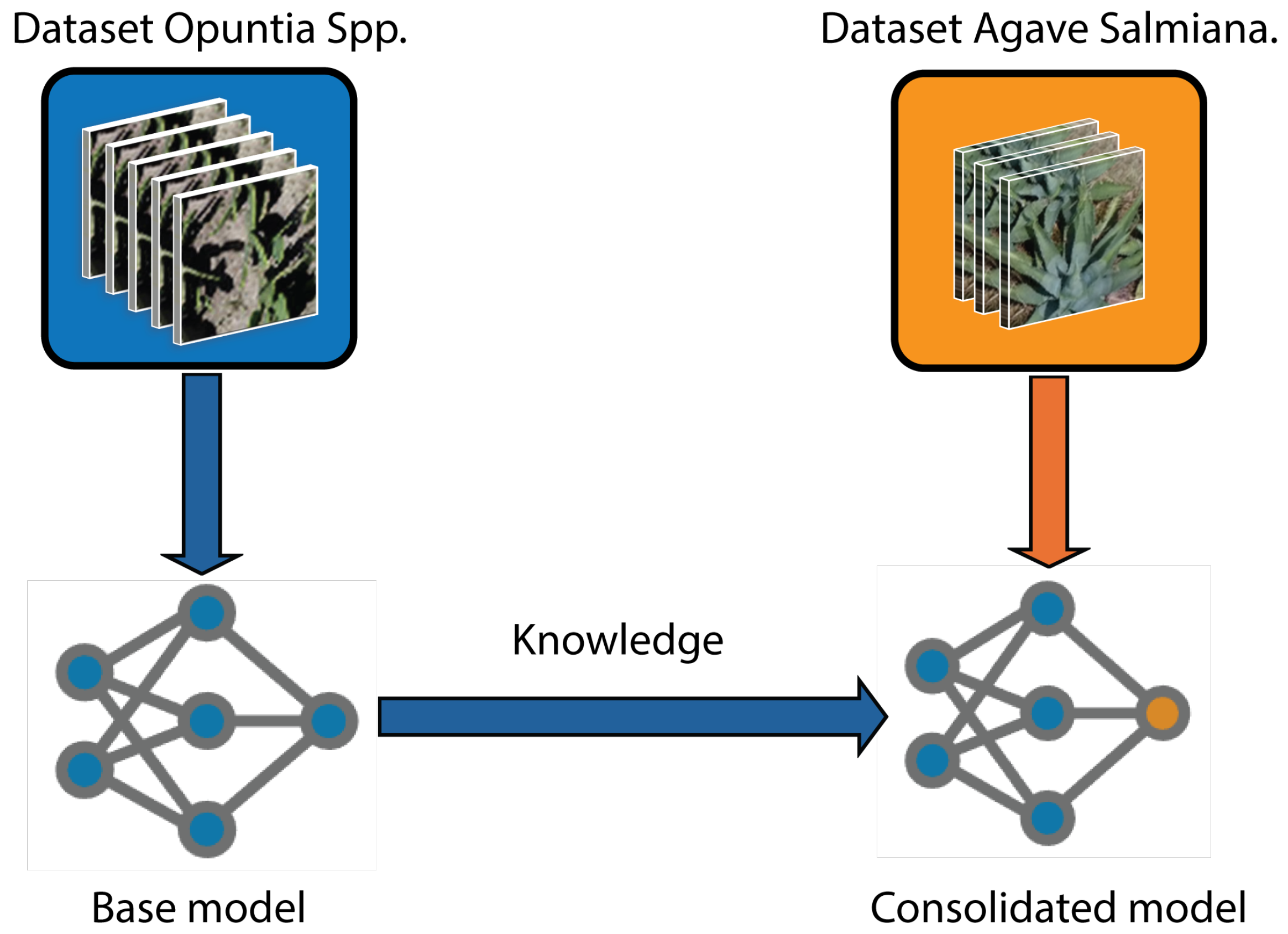
Transfer learning (TL) involves reusing knowledge captured by a previously trained model, typically trained on a broad domain or related tasks, to accelerate convergence and improve generalization in a new scenario with scarce data. Operationally, the most widespread procedure in computer vision is to initialize the weights of the first layers with parameters learned in an abundant set and fine–tune the last layers on the target task (Figure 11). This strategy preserves generic such as edges and textures, thereby focusing specific learning on a reduced subset of parameters and reducing both overfitting and computational.

The usefulness of TL is twofold: on the one hand it alleviates the chronic lack of labeled data, caused by the difficulty of annotating large orthomosaics and the need for experts to validate the classes, and on the other it facilitates adaptation between related domains, for example from one crop to another where plant morphology and lighting conditions differ but share formal color and texture patterns. A recent review quantifies that more than 60% of agricultural studies using Deep Learning already employ some TL scheme, highlighting its role in overcoming labeling and hardware bottlenecks [38].

2.6. Evaluation of Metrics

The experiments were quantitatively evaluated using metrics computed from predicted and reference binary masks, where 1 denotes vegetation pixels and 0 denotes background pixels. Spatial agreement was measured using Intersection over Union (IoU) and the Dice coefficient; global correctness with pixel accuracy; and overall discrepancy with the Root Mean Squared Error (RMSE). Because this study emphasizes boundary delineation, contour quality was additionally evaluated using the Boundary F1 (BF score) and the 95th-percentile Hausdorff distance (HD95) to capture boundary alignment and near-worst-case.

• Intersection over Union (IoU).
  The Intersection over Union (IoU), also known as the Jaccard Index, quantifies the overlap between the predicted mask $M_p$ and the reference mask $M_r$:

  $$\mathrm{IoU}={\displaystyle \frac{|M_p\cap M_r|}{|M_p\cup M_r|}},$$

  (1)

  where $|·|$ denotes the number of pixels in the corresponding set. The metric ranges from 0 (no overlap) to 1 (perfect match) and penalizes both false negatives and false positives, reflecting spatial agreement of vegetation extent.
• Dice coefficient.
  The Dice coefficient measures region overlap with increased sensitivity to agreement in the positive class:

  $$\mathrm{Dice}={\displaystyle \frac{2|M_p\cap M_r|}{|M_p|+|M_r|}},$$

  (2)

  where $|M_p|$ and $|M_r|$ are the number of predicted and reference vegetation pixels, respectively. Dice’s coefficient ranges from 0 to 1, with higher values indicating greater agreement.
• Pixel accuracy.
  Pixel accuracy reports the fraction of correctly classified pixels over the full image:

  $$\mathrm{Acc}={\displaystyle \frac{\mathrm{TP}+\mathrm{TN}}{\mathrm{TP}+\mathrm{TN}+\mathrm{FP}+\mathrm{FN}}},$$

  (3)

  where $\mathrm{TP}$, $\mathrm{TN}$, $\mathrm{FP}$ and $\mathrm{FN}$ denote true positives, true negatives, false positives and false negatives, respectively. Although it can be inflated under class imbalance, it is included as a standard global reference.
• Root Mean Squared Error (RMSE).
  The Root Mean Squared Error (RMSE) measures the average discrepancy between predicted probabilities ${\widehat{y}}_i\in [0,1]$ (or binary predictions) and binary labels $y_i\in \{0,1\}$ over all N pixels:

  $$\mathrm{RMSE}=\sqrt{{\displaystyle \frac{1}{N}}\sum _{i=1}^N{({\widehat{y}}_i-y_i)}^2},$$

  (4)

  where lower values indicate predictions closer to the correct extremes (0 or 1), which is relevant for reliable vegetation cover estimation.
• Boundary F1 (BF score).
  The Boundary F1 (BF score) evaluates contour alignment by comparing boundary pixel sets $B_p$ and $B_r$ (extracted from $M_p$ and $M_r$) under a tolerance $\delta$. Let $d(x,B)={min}_{b\in B}{\parallel x-b\parallel }_2$. Boundary precision and recall are computed as

  $$P_b={\displaystyle \frac{\left|\right\{x\in B_p:d(x,B_r)\le \delta \left\}\right|}{|B_p|}},R_b={\displaystyle \frac{\left|\right\{x\in B_r:d(x,B_p)\le \delta \left\}\right|}{|B_r|}},$$

  (5)

  and combined into

  $$\mathrm{BF}={\displaystyle \frac{2P_b{R}_b}{P_b+R_b}}.$$

  (6)
  This metric emphasizes boundary localization quality while allowing small spatial tolerances.
• 95th-percentile Hausdorff distance (HD95).
  HD95 measures near-worst-case boundary deviation while reducing sensitivity to isolated outliers. Using boundary sets $B_p$ and $B_r$, define point-to-set distances $d(x,B)={min}_{b\in B}{\parallel x-b\parallel }_2$. Then

  $$\mathrm{HD}95=max\left({\mathrm{perc}}_{95}\{d(x,B_r):x\in B_p\},{\mathrm{perc}}_{95}\{d(y,B_p):y\in B_r\}\right),$$

  (7)

  where ${\mathrm{perc}}_{95}\{·\}$ denotes the 95th percentile. HD95 is reported in pixels.

3. Methodology

3.1. Implementation Details

All experiments were carried out on a workstation based on Pop! OS 22.04 LTS, equipped with a 12th generation Intel Core i9–12900K processor (24 threads, up to 5.2 GHz), 32 GB of RAM and an NVIDIA GeForce RTX 4060 Ti GPU with 16 GB GDDR6 memory. The operating system runs on Linux kernel 6.12.10, with CUDA 12.8 support and NVIDIA driver 570.153.02. The station has an x86–64 architecture and was manufactured by Micro–Star International (model MS–7E06). The experiments were conducted in PyCharm using Python 3.10, with PyTorch 2.6.0 and TorchVision 0.21.0 as the primary frameworks. Auxiliary libraries: NumPy (v2.2.6), OpenCV–Python (v4.11.0), and Matplotlib(v3.10.3) were used only for image preprocessing, metric instrumentation, and result visualization.

3.2. Specific Configuration of the Models

All experiments were performed in a binary segmentation setting (NUM_CLASSES = 1) using $224\times 224$ image patches. Data loading was configured with model-dependent batch sizes (4–16) and parallel workers (8–16), while maintaining consistent preprocessing across splits. Data augmentation was primarily geometric (random horizontal/vertical flips with $p=0.5$ and rotations implemented as $\pm {15}^{\circ }$ perturbations or discrete ${90}^{\circ }$ steps), complemented in some configurations by mild photometric jitter (brightness/contrast or ColorJitter) to increase appearance variability without altering the target mask definition.

To compare architectures under controlled conditions, an everyday three-stage schedule was adopted for all seven models: base training (150 epochs), fine-tuning (30 epochs), and consolidation (10 epochs). Learning rates were stage-wise, typically $1\times {10}^{-4}$ for base/fine-tuning and $1\times {10}^{-5}$ for consolidation, with model-specific adjustments (e.g., U-Net Xception-Style used $3\times {10}^{-4}$ in base training and $2\times {10}^{-5}$ in consolidation, and included ReduceLROnPlateau and early stopping). Most models were optimized with AdamW, whereas Swin-UNet used Adam; weight decay was set according to each architecture’s configuration.

Loss functions were defined according to the binary output: U-Net and DeepLabV3+ employed BCEWithLogitsLoss with positive-class weighting ($\mathtt{pos}\_\mathtt{w}=3.0$) combined with a Dice term, SegNet used BCE, and Swin-UNet/SegFormer/Mask2Former used BCEWithLogitsLoss + $0.5$ DiceLoss. Fine-tuning was implemented via partial freezing, training only the task-critical blocks (e.g., decoder/head and late backbone stages) while keeping early encoder/backbone layers fixed; consolidation re-opened all layers for joint optimization at the reduced learning rate. A default probability threshold of 0.5 was used in the base phase; during transfer, U-Net and DeepLabV3+ used a fixed threshold of 0.35, while SegFormer and Mask2Former used a validation-driven sweep in the range 0.30–0.70. Details of the hyperparameter configuration used in this study are summarized in

Table 2. General hyperparameter summary per model. The stage schedule was fixed to T/FT/C = 150/30/10 epochs, where T denotes base training, FT denotes fine-tuning, and C denotes consolidation.

Model	Batch	Opt.	LR	WD	Loss	Thr.	Fine-Tuning (Trainable; Frozen)
Swin–Transformer	4	Adam	T/FT: 1 × 10−4 C: 1 × 10−5	0	BCELogits +0.5Dice	0.5	Head + Stage 3 (freeze Stages 0–2)
SegNet	16	AdamW	T/FT: 1 × 10−4 C: 1 × 10−5	1 × 10−5	BCE	0.5	enc4–enc5 + decoder (freeze enc1–enc3)
UNet–Style–Xception	6	AdamW	T: 3 × 10−4 FT: 1 × 10−4 C: 2 × 10−5	T: 1 × 10−4 FT/C: 1 × 10−5	T: BCELogits+0.5Dice FT/C: BCELogits	0.5	e4–bottleneck + decoders (freeze e1–e3)
DeepLabV3+	8	AdamW	T/FT: 1 × 10−4 C: 1 × 10−5	1 × 10−5	BCELogits($\mathtt{pos}\_\mathtt{w}=3$) + (1-Dice)	T: 0.5 FT/C: 0.35	Head + backbone.layer4 (freeze layer 0–3)
U–Net	8	AdamW	T/FT: 1 × 10−4 C: 1 × 10−5	1 × 10−5	BCELogits($\mathtt{pos}\_\mathtt{w}=3$) + (1-Dice)	T: 0.5 FT/C: 0.35	Bottleneck + decoder + output (freeze enc1–enc4)
SegFormer	4	AdamW	T/FT: 1 × 10−4 C: 1 × 10−5	T: 1 × 10−2 FT/C: 1 × 10−4	BCELogits +0.5Dice	T: 0.5 FT/C: sweep 0.30–0.70	decode_head (freeze encoder)
Mask2Former	4	AdamW	T/FT: 1 × 10−4 C: 1 × 10−5	T: 1 × 10−2 FT/C: 1 × 10−4	BCELogits +0.5Dice	T: 0.5 FT/C: sweep 0.30–0.70	Decoder + heads (freeze backbone + pixel_decoder)

. Full per-model tables (including all stage-wise hyperparameters) are available in the repository at https://github.com/ArturoDuarteR/Semantic-Segmentation-in-Orthomosaics.git (accessed on 20 November 2025).

3.3. Methodological Workflow for Orthomosaic Processing, Model Training, and Vegetation Cover Estimation

The workflow was structured into five sequential phases (Figure 12) that integrate orthomosaic generation, tile-based dataset construction and annotation, and supervised training of CNN- and Transformer-based segmenters, complemented by a knowledge-transfer and consolidation scheme to analyze cross-crop generalization. This methodological design culminates in quantifying vegetation cover at the orthomosaic scale to derive an agronomic indicator from the segmented masks, while preserving consistency across spatial prediction, inter-domain adaptation, and the final estimation of the agronomic parameter.

• Image capture and orthorectification: The RGB acquisition procedure followed the photogrammetric protocol described by Duarte–Rangel et al. [18]. Flights were planned with adequate longitudinal and lateral overlap using a lightweight multirotor UAV to ensure redundancy for accurate reconstruction. Images were processed in WebODM to generate georeferenced orthomosaics that preserve plot geometry and enable subsequent spatially consistent tessellation.
• Preprocessing and dataset enrichment: Before tessellation, black padding was applied to enforce orthomosaic dimensions as exact multiples of the tessellation window. The orthomosaic was then decomposed into non–overlapping tiles ($96\times 96$ px), discarding patches with negligible vegetation to reduce trivial samples. The selected tiles were augmented using moderate geometric transforms (random flips and discrete rotations) and rescaled to $224\times 224$ px to ensure compatibility with pretrained backbones and to standardize the network input across architectures.
• Vegetation cover annotation: Tiles were imported into LabelMe for manual delineation of two semantic categories (plant and background), producing binary ground-truth masks used for supervised optimization and objective evaluation.
• Training, validation, and segmentation: The dataset was partitioned into training, validation, and testing subsets. Models from convolutional encoder–decoder families and Transformer-based designs were trained under a unified training protocol defined as a fixed three-stage schedule: base training on Opuntia (T), fine-tuning on Agave (FT) with partial freezing of early encoder/backbone blocks, and a short consolidation stage (C) with all layers unfrozen at a reduced learning rate for joint optimization. Model performance was quantified using IoU, RMSE, and pixel accuracy, and complemented with Dice, BF score, and HD95 to explicitly characterize region overlap and boundary fidelity; the mean inference time per tile was also recorded.
• Cross–crop transfer, consolidation, and vegetation cover estimation: To assess generalization, models trained on Opuntia spp. were first applied directly to the Agave salmiana orthomosaic (direct inference). Subsequently, fine-tuning was conducted using 6.84% of the Agave orthomosaic tiles (image patches) to adapt the model with limited target-domain supervision, followed by consolidation on the combined (Opuntia+Agave) data. Finally, vegetation cover (leaf area) was estimated from the reconstructed orthomosaic-scale binary masks via pixel counting and GSD conversion, i.e., $A_{\mathrm{veg}}=N_{\mathrm{veg}}·{\mathrm{GSD}}^2$, where $N_{\mathrm{veg}}$ is the number of pixels predicted as vegetation and $\mathrm{GSD}$ is the ground sampling distance of the orthomosaic. The resulting estimates were compared against the manual reference to quantify agreement at the level of the agronomic indicator.

4. Results

This section presents empirical evidence supporting the robustness of the evaluated architectures in the proposed cross-crop setting. First, we establish a baseline by analyzing the performance of models trained on Opuntia spp. and evaluated on its test set. Next, we examine generalization to Agave salmiana through direct (zero-shot) inference and through light fine-tuning with limited target-domain supervision. We then assess the consolidated multi-species checkpoints obtained after a short joint optimization on mixed Opuntia+Agave data, using both region-overlap and boundary-focused metrics to characterize accuracy and contour fidelity. Finally, the consolidated predictions are translated into orthomosaic-scale plant-cover estimates via pixel counting under GSD control, enabling a direct comparison between manual and automatic quantification.

4.1. Performance of the Models Trained on Opuntia spp.

Table 3. Performance on the Opuntia spp. test set.

Metric	Swin–Transformer	SegNet	UNet–Style–Xception	DeepLabV3+	U–Net	SegFormer	Mask2Former
IoU	0.885 ± 0.116	0.597 ± 0.014	0.667 ± 0.008	0.788 ± 0.057	0.678 ± 0.038	0.799 ± 0.0001	0.897 ± 0.094
RMSE	0.167 ± 0.088	0.346 ± 0.006	0.285 ± 0.005	0.228 ± 0.039	0.290 ± 0.021	0.213 ± 0.0001	0.146 ± 0.002
Pixel accuracy	0.965 ± 0.044	0.869 ± 0.006	0.890 ± 0.004	0.934 ± 0.022	0.886 ± 0.016	0.937 ± 0.000	0.968 ± 0.001
$t_{\mathrm{img}}$ (s)	0.0083 ± 0.0185	0.0060 ± 0.000006	0.0029 ± 0.000007	0.0389 ± 0.0075	0.0068 ± 0.0002	0.0007 ± 0.0000	0.0089 ± 0.0000

reports the mean ± standard deviation across test tiles, enabling a joint assessment of central tendency (accuracy) and dispersion (stability) for each architecture. Under this criterion, Mask2Former achieved the highest mean IoU ($0.897$), the lowest RMSE ($0.146$), and the highest pixel accuracy ($0.968$), indicating the best overall agreement with the reference masks while limiting systematic over- and under-segmentation. Importantly, the improvement in mean IoU over the second-best model (Swin–Transformer, $0.885$) is modest ($\Delta$ IoU $\approx 0.012$), whereas the reduction in RMSE is more pronounced ($0.167\to 0.146$), which is consistent with fewer probability/label mismatches concentrated around transition regions (soil–vegetation boundaries). Inference times for Mask2Former and Swin–Transformer are comparable (∼8–9 ms per tile), suggesting that the observed accuracy differences are not driven by a strong speed–accuracy trade-off within this top-performing group.

Beyond average performance, variability differs substantially between models: Swin–Transformer exhibits a larger IoU dispersion ($\pm 0.116$) than Mask2Former ($\pm 0.094$), suggesting higher sensitivity to tile-level heterogeneity (e.g., local illumination changes, mixed pixels, or background texture). SegFormer provides the fastest inference (∼0.7 ms per tile) but with a lower mean IoU (0.799), evidencing a throughput-oriented operating point that may be advantageous for large-scale mapping when minor losses in spatial agreement are acceptable. DeepLabV3+ attains competitive accuracy (IoU 0.788; pixel accuracy 0.934) but at a markedly higher computational cost (38.9 ms per tile), which can become limiting when processing full orthomosaics. Among CNN-based baselines, UNet–Style–Xception yields higher IoU than SegNet and U–Net (0.667 vs. 0.597 and 0.678, respectively) and remains relatively efficient (2.9 ms), supporting its role as a practical compromise; however, the overall ranking indicates that Transformer-based backbones/decoders better capture long-range context and preserve spatial consistency in this dataset, particularly under tile-level variability.

4.2. Knowledge Transfer to Agave (Fine–Tuning)

4.2.1. Direct Inference

Direct inference (i.e., zero-shot transfer) evaluates cross-crop generalization by applying the models trained exclusively on Opuntia spp. to Agave salmiana without updating any weights; therefore, the results in

Table 4. Performance in direct inference on Agave salmiana of the models trained in Opuntia spp.

Metric	Swin–Transformer	SegNet	UNet–Style–Xception	DeepLabV3+	U–Net	SegFormer	Mask2Former
IoU	0.585 ± 0.126	0.628 ± 0.017	0.664 ± 0.007	0.000 ± 0.000	0.559 ± 0.079	0.541 ± 0.001	0.515 ± 0.015
RMSE	0.300 ± 0.132	0.286 ± 0.009	0.255 ± 0.005	0.449 ± 0.057	0.315 ± 0.027	0.325 ± 0.000	0.325 ± 0.009
Pixel accuracy	0.892 ± 0.092	0.907 ± 0.004	0.913 ± 0.003	0.795 ± 0.052	0.860 ± 0.016	0.873 ± 0.000	0.869 ± 0.008
$t_{\mathrm{img}}$ (s)	0.0110 ± 0.0227	0.0109 ± 0.0040	0.0048 ± 0.00004	0.0579 ± 0.0531	0.0093 ± 0.0069	0.007 ± 0.000	0.029 ± 0.000

should be interpreted as a baseline under domain shift (differences in organ geometry, spatial arrangement, background texture, and scale). In this setting, several architectures tend to produce background-dominant predictions, which manifest as near-zero overlap with the reference masks (IoU close to zero) and indicate that the learned decision boundary does not readily translate to agave morphology. In particular, DeepLabV3+ yields an extreme case in which most pixels are assigned to the background class, consistent with a collapse to the majority class under a strong appearance mismatch rather than with a training instability, and highlighting limited out-of-domain transfer for this configuration.

In contrast, other models retain partial transfer capability without target-domain supervision. UNet–Style–Xception attains the highest mean IoU ($0.664\pm 0.007$) and pixel accuracy ($0.913\pm 0.003$), and its low dispersion suggests comparatively stable behavior across tiles, which is compatible with feature extraction that captures morphology-invariant cues (e.g., vegetation texture and boundary evidence) beyond the source crop. SegNet and U–Net also produce non-trivial segmentations, albeit with lower agreement, indicating that their convolutional representations partially extrapolate to the new geometry. Transformer-based models (Swin–Transformer, SegFormer, and Mask2Former) exhibit heterogeneous outcomes in this direct-transfer setting, as reflected by the reported variability and/or reduced agreement, suggesting higher sensitivity to the source–target shift when no adaptation is performed. Overall, these observations motivate the subsequent fine-tuning stage as a controlled mechanism to realign the models to agave appearance while preserving the representations learned on Opuntia.

4.2.2. Fine–Tuning

To adapt the representations learned on Opuntia spp. to the radial morphology of Agave salmiana, fine-tuning was performed for 30 epochs using a reduced learning rate and partial freezing, as described in the Implementation details section. Specifically, the Agave salmiana orthomosaic was tessellated following the same methodological scheme defined for Opuntia, yielding a total of 4900 tiles. Subsequently, applying the same filtering and selection criterion for informative patches (excluding tiles with negligible vegetation), a subset of 335 tiles was extracted to provide limited target-domain supervision. This subset comprises 6.84% of the total number of generated tiles.

Table 5. Performance after fine–tuning on Agave salmiana.

Metric	Swin–Transformer	SegNet	UNet–Style–Xception	DeepLabV3+	U–Net	SegFormer	Mask2Former
IoU	0.741 ± 0.103	0.710 ± 0.012	0.685 ± 0.006	0.772 ± 0.049	0.746 ± 0.064	0.707 ± 0.000	0.754 ± 0.104
RMSE	0.212 ± 0.078	0.243 ± 0.011	0.231 ± 0.003	0.211 ± 0.013	0.209 ± 0.017	0.229 ± 0.001	0.208 ± 0.002
Pixel accuracy	0.949 ± 0.036	0.932 ± 0.003	0.925 ± 0.001	0.947 ± 0.007	0.938 ± 0.011	0.941 ± 0.000	0.951 ± 0.001
$t_{\mathrm{img}}$ (s)	0.0070 ± 0.0010	0.0090 ± 0.0040	0.0030 ± 0.0001	0.0389 ± 0.0075	0.0069 ± 0.0002	0.004 ± 0.000	0.024 ± 0.000

summarizes the metrics obtained after this adaptation.

Fine-tuning on Agave salmiana quantifies adaptation under limited target supervision (30 epochs; 335 tiles, i.e., ≈6.84% of the agave tessellated set), and its effect can be interpreted relative to the direct-inference baseline by inspecting changes in overlap (IoU), discrepancy (RMSE), and variability (standard deviation) reported in Table 5. In this setting, DeepLabV3+ attains the highest mean IoU after adaptation, which is consistent with the capacity of its atrous multiscale representation to recover agave structures once the decision boundary is re-aligned to the target appearance; the contrast with its near-zero IoU under direct inference indicates that its failure mode is dominated by domain shift rather than by insufficient model capacity. Mask2Former, in turn, exhibits the lowest mean error (RMSE) and the highest pixel accuracy after fine-tuning, suggesting a more reliable pixel-level assignment when the model is exposed to agave examples; this behavior is consistent with query-based masked-attention decoding, which refines region predictions under target-domain cues. UNet–Style Xception and SegFormer remain competitive from a computational perspective. Yet, their post-adaptation scores indicate smaller gains in capturing the radial leaf arrangement, suggesting that their representations may require either more target samples or stronger boundary-aware supervision to close the gap. Overall, the fine-tuning results not only increase averages but also differentiate models by adaptation stability (dispersion across tiles) and by the balance between overlap improvement and error reduction, thereby providing a technical basis for selecting architectures based on accuracy requirements and orthomosaic-scale deployment constraints.

4.3. Intercropping Consolidation (Opuntia spp. + Agave salmiana)

After completing the consolidation stage (C), a single consolidated multi-species model was obtained for each architecture, i.e., one final checkpoint per model family. This phase consisted of 10 training epochs using a 1:1 mixture of prickly pear and agave images, with a uniform learning rate of $1\times {10}^{-5}$ across all models. The goal was to preserve the knowledge previously acquired on prickly pear while simultaneously stabilizing performance on agave, thereby mitigating catastrophic forgetting and encouraging a shared representation across species. To assess the consolidated models, we report IoU, RMSE, pixel accuracy, and mean inference time, and additionally Dice, Boundary F1 (BF score), and HD95 to explicitly characterize region overlap and boundary fidelity. Crop-wise results are provided in

Table 6. Performance on Opuntia spp. after intercropping consolidation.

Metric	Swin–Transformer	SegNet	UNet–Style–Xception	DeepLabV3+	U–Net	SegFormer	Mask2Former
IoU	0.879 ± 0.116	0.713 ± 0.046	0.625 ± 0.010	0.758 ± 0.053	0.660 ± 0.038	0.792 ± 0.000	0.894 ± 0.004
RMSE	0.172 ± 0.087	0.265 ± 0.025	0.293 ± 0.003	0.249 ± 0.037	0.293 ± 0.021	0.246 ± 0.001	0.155 ± 0.005
Pixel accuracy	0.963 ± 0.045	0.906 ± 0.021	0.878 ± 0.003	0.923 ± 0.022	0.876 ± 0.017	0.935 ± 0.000	0.967 ± 0.001
Dice	0.950 ± 0.035	0.736 ± 0.070	0.757 ± 0.068	0.900 ± 0.051	0.796 ± 0.050	0.902 ± 0.032	0.956 ± 0.036
BF score	0.952 ± 0.103	0.385 ± 0.059	0.429 ± 0.066	0.782 ± 0.153	0.425 ± 0.057	0.752 ± 0.083	0.962 ± 0.102
HD95 (px)	2.759 ± 3.391	22.624 ± 11.303	20.771 ± 10.419	7.947 ± 7.758	18.276 ± 6.764	8.724 ± 5.283	2.189 ± 3.447
$t_{\mathrm{img}}$ (s)	0.0073 ± 0.0009	0.0086 ± 0.0035	0.0029 ± 0.0001	0.0398 ± 0.0050	0.0069 ± 0.0001	0.0042 ± 0.0001	0.0237 ± 0.0001

and

Table 7. Performance on Agave salmiana after intercropping consolidation.

Metric	Swin–Transformer	SegNet	UNet–Style–Xception	DeepLabV3+	U–Net	SegFormer	Mask2Former
IoU	0.738 ± 0.106	0.700 ± 0.010	0.719 ± 0.003	0.756 ± 0.055	0.721 ± 0.032	0.715 ± 0.000	0.760 ± 0.046
RMSE	0.212 ± 0.077	0.235 ± 0.006	0.217 ± 0.002	0.219 ± 0.029	0.226 ± 0.018	0.224 ± 0.001	0.208 ± 0.002
Pixel accuracy	0.949 ± 0.035	0.929 ± 0.004	0.933 ± 0.001	0.940 ± 0.017	0.932 ± 0.014	0.943 ± 0.001	0.951 ± 0.001
Dice	0.924 ± 0.068	0.818 ± 0.097	0.793 ± 0.118	0.915 ± 0.076	0.877 ± 0.066	0.836 ± 0.077	0.922 ± 0.079
BF score	0.873 ± 0.162	0.473 ± 0.097	0.476 ± 0.107	0.834 ± 0.167	0.666 ± 0.136	0.571 ± 0.098	0.877 ± 0.153
HD95 (px)	8.362 ± 17.086	29.587 ± 26.400	30.864 ± 29.226	11.427 ± 14.699	20.499 ± 22.562	24.217 ± 23.772	8.458 ± 16.667
$t_{\mathrm{img}}$ (s)	0.0072 ± 0.0004	0.0086 ± 0.0036	0.0028 ± 0.0002	0.0051 ± 0.0007	0.0069 ± 0.0001	0.0041 ± 0.0001	0.0237 ± 0.0001

.

The intercropping consolidation phase allowed evaluating the ability of the models to operate jointly on both crops after a cross–crop adjustment. This assessment was performed using region-based metrics (IoU and Dice), global correctness (pixel accuracy), discrepancy (RMSE), and boundary-focused criteria (BF score and HD95) reported in Table 6 and Table 7. In Opuntia spp., the best performance was achieved by Mask2Former, with the highest IoU and accuracy, as well as the lowest mean error. Consistently, it also achieved the highest Dice and BF score and the lowest HD95, indicating superior boundary fidelity in the consolidated setting; moreover, its IoU variability is minimal (±0.004), suggesting stable behavior across tiles. These results suggest that attention-based decoders can integrate multi-species variability while preserving contour alignment, whereas several CNN/hybrid baselines exhibit weaker boundary localization (lower BF score and larger HD95) despite comparable coarse overlap in some cases. In contrast, UNet–Style–Xception and U–Net showed notably lower IoU and accuracy, indicating limited generalization capacity under multicrop scenarios. This limitation is further reflected in their boundary metrics (lower BF score and substantially higher HD95), which indicates larger contour deviations after consolidation.

In Agave salmiana, a more balanced distribution was observed. Specifically, mean IoU values are more tightly clustered (approximately 0.700–0.760) after consolidation, relative to direct inference. Within this range, Mask2Former attains the highest IoU, while DeepLabV3+ remains competitive in overlap (IoU 0.756 ± 0.055), consistent with multiscale representations supporting radial structures after adaptation. However, Mask2Former again stood out in reducing error and in overall accuracy, confirming that its strength lies in more precise pixel–level classification. In addition, boundary-focused metrics further differentiate models with similar IoU: Mask2Former (and Swin–Transformer) provides the highest BF scores and the lowest HD95 values, although HD95 exhibits large dispersion across models, indicating tile-level heterogeneity in agave plots. Models such as Swin–Transformer and SegFormer achieved acceptable performance, although without excelling in key metrics, while the CNN baselines generally show lower boundary fidelity (BF score/HD95) than the best attention-based configurations under the consolidated multi-crop setting.

The multi-species models obtained after consolidation enable analyzing performance under an operational scenario in which both morphologies coexist. As shown in

Table 8. Evolution of the process (IoU ± standard deviation) throughout the four stages: base training in Opuntia spp., direct inference in Agave salmiana, fine–tuning in agave and intercropping consolidation.

Model	Base Prickly Pear	Inference Agave	Fine–Tuning Agave	Consolidation Prickly Pear	Consolidation Agave
Swin–Transformer	0.885 ± 0.116	0.585 ± 0.126	0.741 ± 0.103	0.879 ± 0.116	0.738 ± 0.106
SegNet	0.597 ± 0.014	0.628 ± 0.017	0.710 ± 0.012	0.713 ± 0.046	0.700 ± 0.010
UNet–Style–Xception	0.667 ± 0.008	0.664 ± 0.007	0.685 ± 0.006	0.625 ± 0.010	0.719 ± 0.003
DeepLabV3+	0.788 ± 0.057	0.000 ± 0.000	0.772 ± 0.049	0.758 ± 0.053	0.756 ± 0.055
U–Net	0.678 ± 0.038	0.559 ± 0.079	0.746 ± 0.064	0.660 ± 0.038	0.721 ± 0.032
SegFormer	0.799 ± 0.001	0.541 ± 0.001	0.707 ± 0.000	0.792 ± 0.000	0.715 ± 0.000
Mask2Former	0.897 ± 0.094	0.515 ± 0.015	0.754 ± 0.104	0.894 ± 0.004	0.760 ± 0.046

, Mask2Former sustains the highest overlap (IoU) on both crops after consolidation, while

Table 9. Boundary-focused metrics after intercropping consolidation.

Metric	Swin–Transformer	SegNet	UNet–Style–Xception	DeepLabV3+	U–Net	SegFormer	Mask2Former
Dice (Opuntia)	0.950 ± 0.035	0.736 ± 0.070	0.757 ± 0.068	0.900 ± 0.051	0.796 ± 0.050	0.902 ± 0.032	0.956 ± 0.036
BF score (Opuntia)	0.952 ± 0.103	0.385 ± 0.059	0.429 ± 0.066	0.782 ± 0.153	0.425 ± 0.057	0.752 ± 0.083	0.962 ± 0.102
HD95 (px) (Opuntia)	2.759 ± 3.391	22.624 ± 11.303	20.771 ± 10.419	7.947 ± 7.758	18.276 ± 6.764	8.724 ± 5.283	2.189 ± 3.447
Dice (Agave)	0.924 ± 0.068	0.818 ± 0.097	0.793 ± 0.118	0.915 ± 0.076	0.877 ± 0.066	0.836 ± 0.077	0.922 ± 0.079
BF score (Agave)	0.873 ± 0.162	0.473 ± 0.097	0.476 ± 0.107	0.834 ± 0.167	0.666 ± 0.136	0.571 ± 0.098	0.877 ± 0.153
HD95 (px) (Agave)	8.362 ± 17.086	29.587 ± 26.400	30.864 ± 29.226	11.427 ± 14.699	20.499 ± 22.562	24.217 ± 23.772	8.458 ± 16.667

indicates that it also preserves high boundary fidelity through a strong BF score and a low HD95. This joint behavior is decisive when vegetation cover is estimated via pixel counting at orthomosaic scale. For this reason, the consolidated Mask2Former model was adopted for the final cover quantification and for computing the derived agronomic indicator, since spatially coherent contours reduce over-/under-estimation bias in soil–vegetation transition zones.

4.4. Quantification of Plant Cover

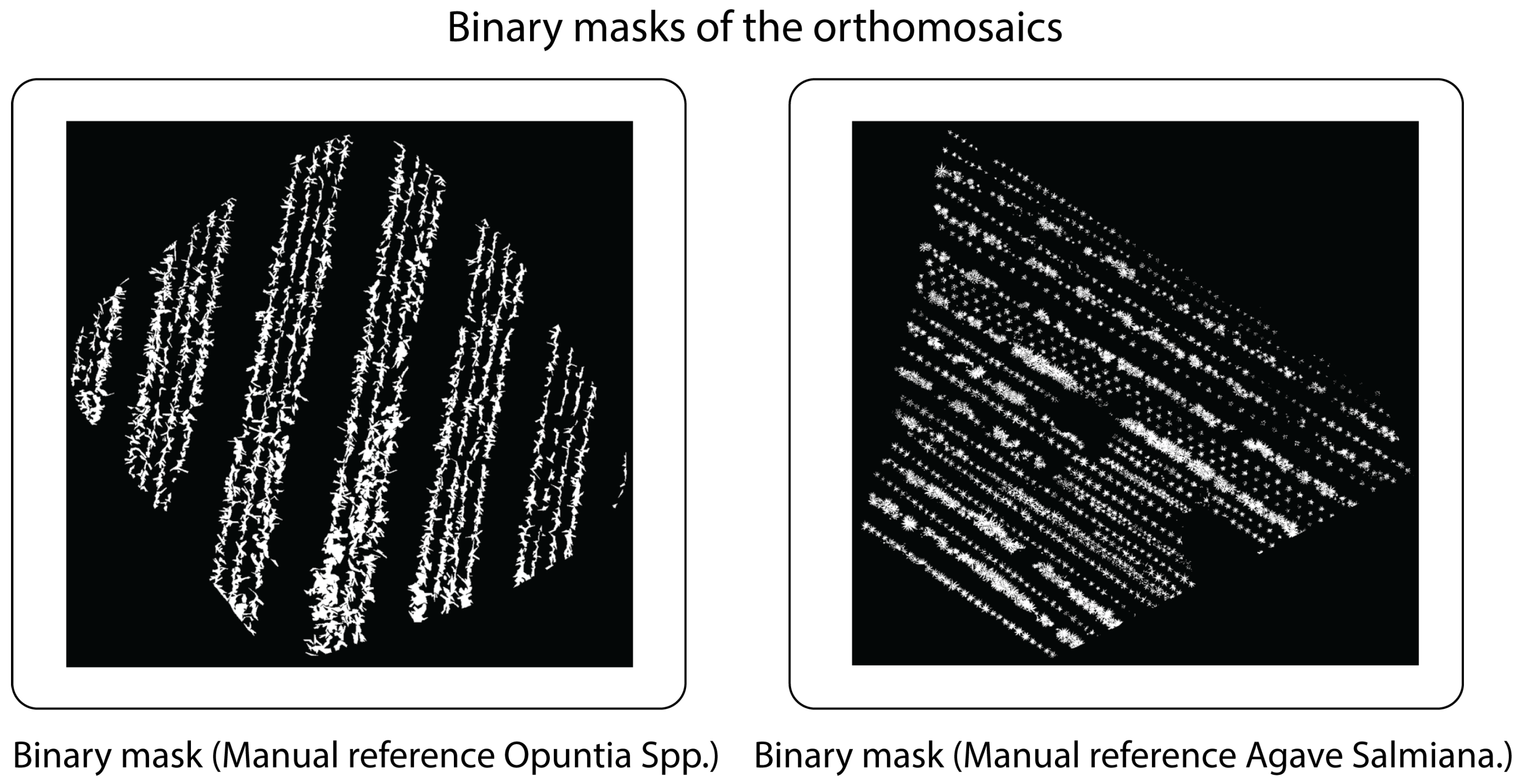
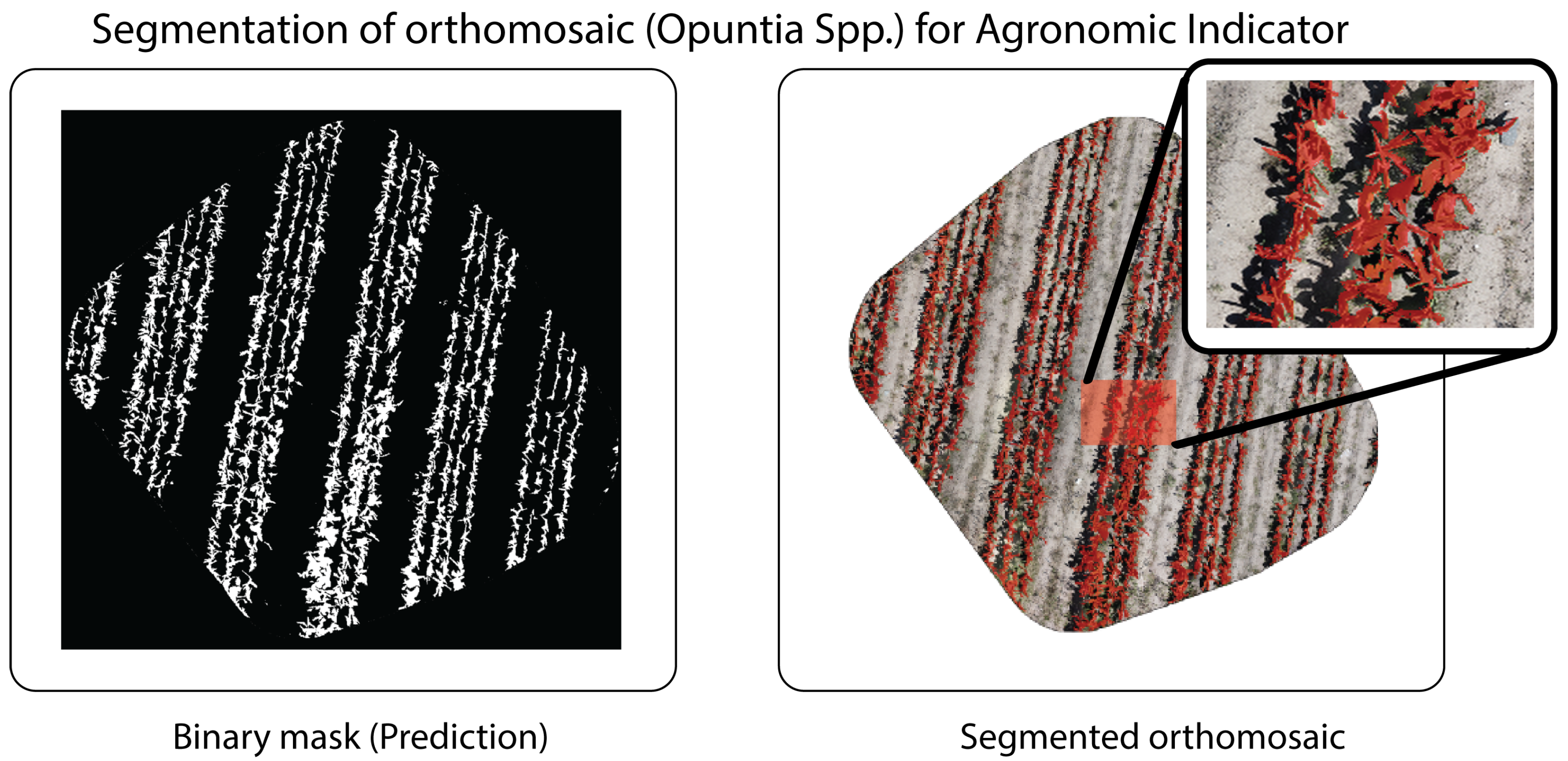
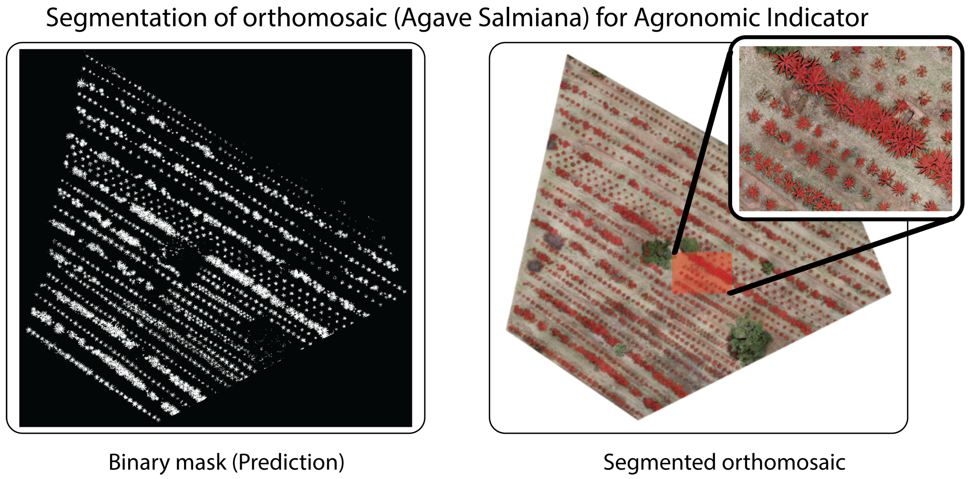
Plant cover quantification was performed using reference masks generated by manual annotation in LabelMe on each orthomosaic (both Opuntia spp. and Agave salmiana), establishing a binary classification {vegetation, background} (Figure 13).

These masks served as the baseline for estimating leaf area by direct pixel counting and converting pixel counts to area units based on the ground sample distance (GSD) specific to each orthomosaic. Operationally, if $N_{\mathrm{veg}}$ denotes the number of pixels labeled as vegetation and GSD the resolution in meters per pixel, the covered area was obtained as:

$$A_{\mathrm{veg}}\left[{\mathrm{m}}^2\right]=N_{\mathrm{veg}}\times {\mathrm{GSD}}^2.$$

(8)

To compare manual and automatic quantification, Mask2Former was selected as the reference architecture, given its consolidated multi-species performance and its favorable boundary fidelity. Concordance between the two approaches was assessed beyond tile-level segmentation metrics by considering an agronomic indicator derived at orthomosaic scale: leaf area. Specifically, the absolute difference $\Delta A=|A_{\mathrm{veg}}^{\mathrm{pred}}-A_{\mathrm{veg}}^{\mathrm{ref}}|$ and the relative percentage error

$${\epsilon }_{\%}=100\times {\displaystyle \frac{|A_{\mathrm{veg}}^{\mathrm{pred}}-A_{\mathrm{veg}}^{\mathrm{ref}}|}{A_{\mathrm{veg}}^{\mathrm{ref}}}},$$

(9)

were calculated, where $A_{\mathrm{veg}}^{\mathrm{pred}}$ comes from the mask segmented by Mask2Former and $A_{\mathrm{veg}}^{\mathrm{ref}}$ from the manual mask. The aggregated results are presented in Table 10.

Table 10. Crop–by–crop comparison between the coverage estimated by Mask2Former and the manual reference. The vegetation pixels in both masks, the resulting areas and the absolute and relative area errors are reported.

Crop	GSD (cm/px)	${\mathit{N}}_{\mathbf{px}}^{\mathbf{pred}}$	${\mathit{N}}_{\mathbf{px}}^{\mathbf{ref}}$	${\mathit{A}}_{\mathbf{veg}}^{\mathbf{pred}}$ (m2)	${\mathit{A}}_{\mathbf{veg}}^{\mathbf{ref}}$ (m2)	$\mathbf{\Delta }\mathit{A}$ (m2)	${\mathit{\epsilon }}_{\%}$
Opuntia spp. (Figure 14)	1.02	527,192	516,209	55.39	54.23	1.15	2.13
Agave salmiana (Figure 15)	1.80	3,550,260	3,541,399	1150.28	1147.41	2.87	0.25

Table 10. Crop–by–crop comparison between the coverage estimated by Mask2Former and the manual reference. The vegetation pixels in both masks, the resulting areas and the absolute and relative area errors are reported.

Crop	GSD (cm/px)	${\mathit{N}}_{\mathbf{px}}^{\mathbf{pred}}$	${\mathit{N}}_{\mathbf{px}}^{\mathbf{ref}}$	${\mathit{A}}_{\mathbf{veg}}^{\mathbf{pred}}$ (m2)	${\mathit{A}}_{\mathbf{veg}}^{\mathbf{ref}}$ (m2)	$\mathbf{\Delta }\mathit{A}$ (m2)	${\mathit{\epsilon }}_{\%}$
Opuntia spp. (Figure 14)	1.02	527,192	516,209	55.39	54.23	1.15	2.13
Agave salmiana (Figure 15)	1.80	3,550,260	3,541,399	1150.28	1147.41	2.87	0.25

Vegetation-cover estimation at orthomosaic scale depends directly on counting pixels classified as vegetation $A_{\mathrm{veg}}=N_{\mathrm{veg}}·{\mathrm{GSD}}^2$; therefore, its validity should be interpreted jointly with overlap metrics (IoU, Dice) and contour metrics (BF score, HD95), in addition to RMSE and pixel accuracy. In particular, while IoU/Dice reflect regional agreement, BF score and HD95 explain area bias, since small boundary misalignments in soil–vegetation transitions or thin structures translate into peripheral false positives/negatives that accumulate in $\Delta A$ and ${\epsilon }_A$. Consequently, residual discrepancies in the agronomic indicator tend to concentrate in regions of leaf occlusion/overlap and radiometrically ambiguous edges (shadows, soil texture), where the class–background separation is less stable. Under this criterion, architectures are prioritized that, in addition to maximizing overlap, maintain high contour fidelity, because this directly reduces the systematic error of the estimated cover.

5. Discussion

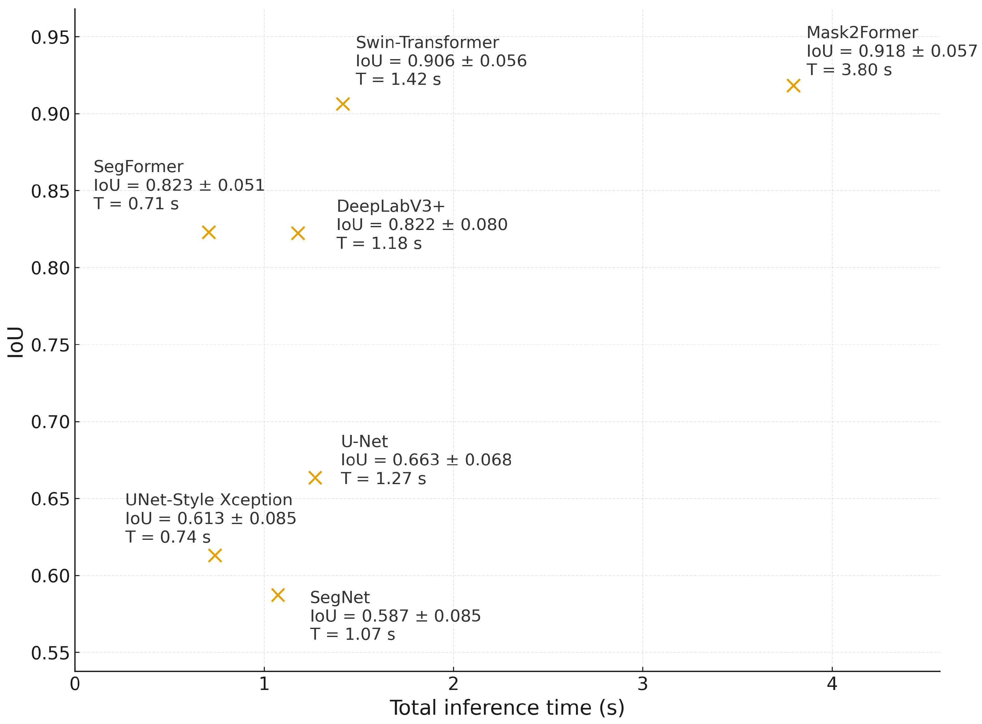
The results show a differentiable behavior depending on crop morphology and confirm a trade–off between precision and inference cost that, in our case, must be resolved in favor of precision. In Opuntia spp., the IoU–time relationship in Figure 16 shows that Mask2Former achieves the highest IoU, while Swin–Transformer comes close with a shorter latency. However, because the end-use objective is orthomosaic-scale cover quantification, the decision should prioritize segmentation fidelity over marginal latency reductions: a higher IoU translates into a more realistic agronomic indicator (plant cover). DeepLabV3+ and SegFormer form intermediate options: their IoU is competitive in prickly pear, and although SegFormer offers lower latency, that benefit does not justify sacrificing accuracy when the objective is to derive management metrics from segmentation. Classic CNNs (U–Net, U–Net Style Xception, and SegNet) achieve lower IoU scores, consistent with limitations in preserving fine edges and spatial continuity during tessellation.

Beyond the IoU–time trade-off, the inclusion of boundary-oriented criteria (BF score and HD95) provides complementary evidence on contour stability, which is critical when cover is computed by pixel counting at orthomosaic scale. Specifically, Dice/IoU quantify regional agreement, whereas BF score and HD95 capture contour alignment and near-worst-case boundary deviations, respectively; therefore, models with similar IoU can still differ in the systematic bias that propagates into leaf-area estimation. In Opuntia, this distinction is operationally relevant because pad boundaries are often fragmented by shadows and soil texture; accordingly, architectures that preserve spatially coherent contours (Table 9) are preferable when the final objective of the pipeline is an agronomic indicator rather than tile-level agreement alone.

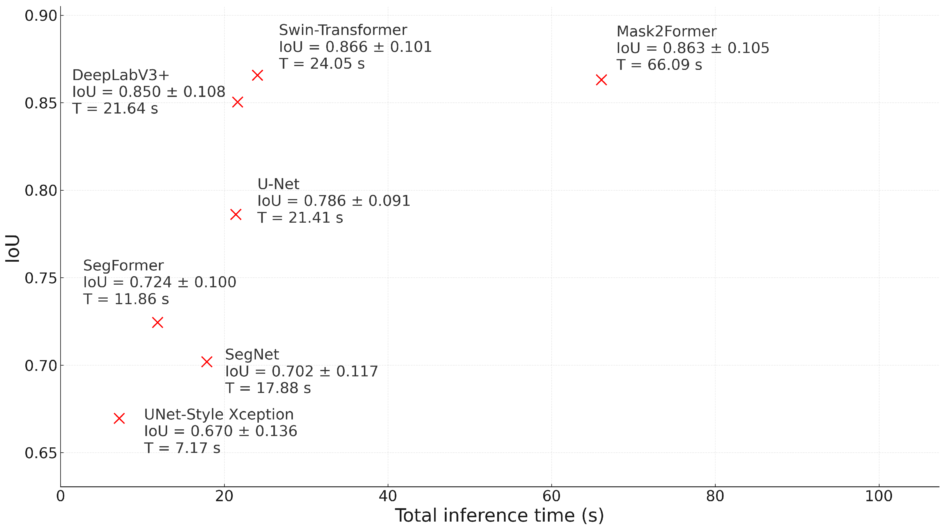
In Agave salmiana, Figure 17 reveals complementary strengths: DeepLabV3+ and Swin–Transformer achieve IoU similar or very close to Mask2Former with shorter times. However, maintaining the previous criterion, the methodological decision must be guided by IoU, as these are radial crowns with more marked texture transitions, small precision losses have a magnified effect on leaf area estimation. In this scenario, Mask2Former remains a reference due to its spatial coherence and stability, while DeepLabV3+ excels at capturing radial patterns, and Swin–Transformer maintains high, consistent performance. SegFormer maintains the best speed/IoU ratio, which is useful when latency is a hard constraint; however, the priority for building a direct agronomic indicator should remain accuracy.

For agave, the boundary metrics help to interpret why architectures that are competitive in IoU may still yield different area errors: radial leaf arrangements increase the proportion of boundary pixels, making small contour shifts accumulate in peripheral false positives/negatives. Under these conditions, the HD95 and BF scores serve as informative complements to IoU/Dice, as they characterize the stability of crown edges and the extent of boundary outliers in radiometrically ambiguous zones (e.g., shadows and soil texture), which are common in semi-arid orthomosaics. Consequently, selecting a model for area estimation benefits from jointly considering overlap and boundary fidelity rather than relying on IoU alone.

The cross–domain analysis supports the need for a transfer cycle with consolidation. Direct inference shows selective degradations when changing morphology (prickly pear → agave), while light fine–tuning, followed by multi–species consolidation, stabilizes performance and reduces incremental relabeling. Together, the findings suggest a practical guideline: first, prioritize attention models to ensure spatial coherence and robustness in Opuntia; second, consider DeepLabV3+ and Swin–Transformer as high–precision alternatives in Agave, without renouncing Mask2Former when the main objective is to maximize IoU; and third, reserve latency arguments for scenarios where the processing window is strict, since, under normal conditions, the total time per orthomosaic does not displace precision as the leading criterion.

From an operational perspective, the orthomosaic-scale pipeline and traceability, from pixel–to–pixel prediction to leaf-area estimation, enable the model output to serve as a direct agronomic indicator. Under this framework, minor improvements in IoU have a multiplicative effect on estimator quality, reinforcing the convenience of selecting architectures based on their precision performance rather than marginal advantages in latency.

The observed patterns are consistent with prior evidence in agricultural segmentation: CNN baselines can be effective under controlled domains, yet robustness and contour preservation degrade under heterogeneous conditions and domain shifts [18,39]. In weed mapping and crop–weed delineation, SegNet-type approaches have shown practical value, particularly when complementary spectral cues (e.g., NDVI) strengthen vegetation discrimination [40]; however, recent UAV-based evaluations also report that Transformer families (e.g., SegFormer) can maintain robust performance across lighting and texture variability [41]. In this study, the advantage of attention-driven models becomes more evident when performance is evaluated using boundary-aware criteria (BF score, HD95) in addition to overlap metrics, because these metrics better reflect contour accuracy and transfer stability–two properties that directly govern orthomosaic-scale cover estimation and its derived agronomic indicators.

6. Limitations and Future Work

This study provides a controlled comparison of CNN- and Transformer-based segmenters on UAV RGB orthomosaics of Opuntia spp. and Agave salmiana; however, several factors constrain the scope of the conclusions. The experiments are based on a limited number of orthomosaics and compact tile datasets, and the annotation is formulated as binary segmentation (plant vs. background) using RGB imagery only. This setup is adequate for estimating vegetation cover but does not explicitly represent other agronomically relevant elements, such as weeds, residues, or shadow classes. In addition, the patch-based workflow adopted for training and inference is practical and reproducible. Yet, it can attenuate long-range context and tends to concentrate residual discrepancies around soil–vegetation transitions and thin structures, which motivates complementing overlap metrics with boundary-sensitive criteria when interpreting area estimates.

As future work, we recommend extending the evaluation to additional fields and acquisition conditions (dates, phenological stages, illumination, and soil-texture variability) to strengthen the evidence of generalization. It is also relevant to move beyond binary segmentation toward multi-class or instance-aware formulations (crop/weed/soil/shadow) and, when available, to incorporate complementary spectral information, together with radiometric normalization, to reduce ambiguity in shadowed regions and heterogeneous backgrounds. Methodologically, overlapping tiling and explicit boundary-refinement strategies should be assessed to stabilize orthomosaic-scale contours, along with label-efficient adaptation approaches (active learning or self-supervised pretraining) to reduce annotation cost. Finally, progressively integrating additional morphologically related crops would enable broader multi-species models and advance toward unified cover estimation in semi-arid production systems.

7. Conclusions

This study confirms that cross-crop transfer from Opuntia spp. to Agave salmiana is feasible when geometric standardization with pixel–to–surface traceability (via GSD), a brief domain adaptation stage, and a subsequent consolidation step are enforced at orthomosaic scale. The need for explicit adaptation is evidenced by the marked domain-shift sensitivity observed under direct inference, in which DeepLabV3+ achieved an IoU of 0.000 ± 0.000 on agave before adaptation. In contrast, fine–tuning and consolidation recovered competitive performance, reaching IoU $0.772\pm 0.049$ after fine–tuning and IoU $0.756\pm 0.055$ after consolidation.

After intercropping consolidation, Mask2Former exhibited the most consistent multi-species behavior, attaining the highest IoU on both crops (IoU $0.894\pm 0.004$ on Opuntia and IoU $0.760\pm 0.046$ on Agave). Boundary-aware evaluation further supports its suitability for orthomosaic-scale cover quantification: Mask2Former achieved BF score $0.962\pm 0.102$ and HD95 $2.189\pm 3.447$ px on Opuntia, and BF score $0.877\pm 0.153$ with HD95 $8.458\pm 16.667$ px on Agave, indicating high contour alignment in both morphologies. Although other architectures can be competitive on individual criteria, Mask2Former exhibits the most favorable joint performance across overlap and contour fidelity, which is decisive when vegetation cover is computed by pixel counting and subsequently converted to leaf area.

Overall, the proposed orthomosaic-scale protocol provides a reproducible framework for training, adapting, and auditing segmentation models for semi-arid succulent crops, thereby translating segmentation outputs into traceable vegetation-cover indicators. Beyond overlap and discrepancy metrics (IoU, RMSE, pixel accuracy), incorporating boundary-sensitive indicators (BF score, HD95) is necessary to ensure that model improvements correspond to reduced contour-driven bias in coverage estimation and, consequently, to more reliable agronomic indicators derived from the masks.