Article

Hybrid Digital Twin for Phytotron Microclimate Control: Integrating Physics-Based Modeling and IoT Sensor Networks

by
Vladimir V. Bukhtoyarov
1,2,3,
Ivan S. Nekrasov
2,*,
Ivan A. Timofeenko
4,
Alexey A. Gorodov
2,
Stanislav A. Kartushinskii
4,5,
Yury V. Trofimov
6 and
Sergey I. Lishik
6
1
Laboratory of Biofuel Compositions, Siberian Federal University, 660041 Krasnoyarsk, Russia
2
Department of Technological Machines and Equipment of Oil and Gas Complex, School of Petroleum and Natural Gas Engineering, Siberian Federal University, 660041 Krasnoyarsk, Russia
3
Artificial Intelligence Technology Scientific and Education Center, Bauman Moscow State Technical University, 105005 Moscow, Russia
4
Interdisciplinary Laboratory of City Farming, Institute of Gastronomy, Siberian Federal University, 660041 Krasnoyarsk, Russia
5
School of Space and Information Technology, Siberian Federal University, 660041 Krasnoyarsk, Russia
6
Center LED and Optoelectronics Technologies of National Academy Sciences of Belarus, 220090 Minsk, Belarus
*
Author to whom correspondence should be addressed.
AgriEngineering 2025, 7(9), 285; https://doi.org/10.3390/agriengineering7090285
Submission received: 26 June 2025 / Revised: 19 August 2025 / Accepted: 21 August 2025 / Published: 2 September 2025

Abstract

Integration of IoT and predictive modeling is critical for optimizing microclimate management in urban-agglomeration vertical farming. In this study, we present a hybrid digital twin approach that combines a physical microclimate model with a distributed IoT monitoring system to simulate and control the phytotron environment. A set of heat- and mass-balance equations governing the dynamics of temperature, humidity, and transpiration was implemented and parameterized using a genetic algorithm (GA)—an evolutionary optimization method—with real-time data collected over three intervals (72 h, 90 h, and 110 h) from LoRaWAN sensors (temperature, humidity, CO2) and Wi-Fi-connected power meters managed by Home Assistant. The optimized model achieved mean temperature deviations ≤ 0.1 °C, relative humidity errors ≤ 2%, and overall energy consumption accuracy of 99.5% compared to measured values. The digital twin reliably tracked daily climate fluctuations and system energy use, confirming the accuracy of the hybrid approach. These results demonstrate that the proposed framework effectively integrates theoretical models with IoT-derived data to deliver precise environmental control and energy-use optimization in vertical farming, while also laying the groundwork for scalable digital twins in controlled-environment agriculture.

1. Introduction

In recent years, the Internet of Things has become one of the main driving forces behind the digitalization of agriculture. The concept of “smart farming,” or Agriculture 4.0, entails the widespread deployment of sensor networks and connected devices to monitor growing conditions and automate cultivation processes [1]. Studies show that applying IoT technology in agricultural systems makes it possible to collect real-time data on key environmental parameters (temperature, humidity, illuminance, CO2 concentration, soil or substrate moisture, etc.) and, on that basis, to regulate resource use with high precision [2,3]. Thanks to such IoT systems, water, fertilizer, and energy are used more efficiently, waste is minimized, and optimal conditions for plant growth are maintained [4].
The role of IoT is especially significant in urban-agglomeration vertical farms—multi-tiered installations for growing plants in controlled environments. In land-constrained city settings, these vertical farms rely on hydroponic or aeroponic technologies and are entirely dependent on electronic control systems. Networks of sensors and actuators continuously monitor the microclimate at each level of the farm, automatically maintaining the required growing conditions. For example, light sensors can track illuminance levels and activate adaptive LED lighting to provide the precise spectrum and intensity needed for each crop [5,6]. Similarly, humidity and air-temperature sensors, together with intelligent controllers, manage irrigation, ventilation, and heating systems to ensure a stable climate [7]. Integrating IoT into these processes delivers tangible benefits. Resource use becomes more targeted (water, nutrient solutions), energy and labor costs drop, and both productivity and production resilience increase.
Moreover, comprehensive IoT architectures are being developed specifically for vertical farms. For instance, Monteiro et al. proposed an IoT framework for vertical farming within sustainable controlled-environment agriculture [8]. Such a system comprises numerous sensors and a cloud infrastructure for data collection and analysis, enabling real-time monitoring of each farm tier and rapid response to deviations [9]. Various communication protocols are employed: Wi-Fi, Bluetooth, ZigBee, and Z-Wave for short-range links; and LoRaWAN, NB-IoT, and Sigfox for wide-area, low-power connectivity [10,11].
Overall, IoT technologies have become an integral part of urban vertical farming, laying the foundation for automation and precision agriculture in cities. Nevertheless, challenges remain. Reliable wireless communication protocols are needed, common standards for device interoperability must be established, and solutions for real-time processing of large sensor data streams must be developed. These issues are gradually being addressed as agro-IoT matures, but most studies emphasize that IoT integration should be accompanied by robust analytics and secure data storage to fully realize the potential of smart farming technologies [12].
Microclimate control is a key success factor for vertical farms and other controlled-environment agriculture systems. The speed of crop growth and final yield depend directly on maintaining optimal conditions. Accordingly, in recent years, numerous solutions have appeared aiming to fully automate microclimate management in greenhouses and vertical farms. Traditional climate-control systems (as used in commercial greenhouses) are evolving with the addition of IoT sensors and intelligent algorithms, enabling real-time environmental regulation without human intervention.
Modern researchers propose various approaches to microclimate automation. One trend is the use of climate models and simulations to predict and optimize growing conditions [13]. This highlights the importance of predictive models; if the control system can compute how a change in, say, temperature or lighting will affect plant growth, it can proactively adjust those parameters for better outcomes [14]. Examples of such model-driven automation are already emerging in vertical farms. For instance, the iFarm platform combines IoT sensors with automated climate control supported by neural network algorithms to maintain stable, year-round conditions without pesticides [15]. In this system, a neural network evaluates biomass growth dynamics, camera data are analyzed by a chatbot to detect developmental anomalies, and environmental parameters are then automatically adjusted.
Another aspect of microclimate automation is energy efficiency and precision control. Since vertical farms consume substantial resources (electricity for lighting and climate systems), optimizing their operation is critical. Research in this area focuses on algorithms that strike a balance between optimal plant conditions and minimal energy expenditure [16]. For example, dynamic LED lighting control systems adjust spectrum and brightness according to plant growth stage and time of day, saving energy without compromising photosynthesis. Likewise, ventilation and air-conditioning systems can be managed by predictive models. Knowing the weather forecast or diurnal temperature cycles, the controller pre-emptively alters operation to prevent abrupt climate fluctuations within the closed ecosystem. Thus, studies agree that autonomous climate-control systems with AI elements can significantly enhance vertical farm efficiency.
It is important to note that microclimate management is increasingly being integrated with the digital twin concept. In other words, alongside traditional sensors and controllers, a software model of the farm is introduced that “mirrors” its state and allows testing of various control scenarios. This approach in vertical farming is implemented through an algorithmic loop: physical sensors feed data into the virtual farm model, where climate change scenarios are computed, and optimal control strategies are selected and then applied in the real system. This paves the way for the next research direction—applying digital twins for simulation modeling of agri-systems.
The concept of a digital twin in agriculture has emerged relatively recently but is already seen as a promising tool for production optimization [17]. A digital twin is a virtual replica of a real object (in our case, a farm or its components) that continuously synchronizes with it via sensor data and enables in silico analysis of system states, prediction of changes, and selection of optimal actions. In other words, a digital twin is a dynamic computational model of the farm updated in real time, used for monitoring, virtual experimentation, and decision support. Thanks to integration with IoT devices, the twin receives up-to-date information about the ecosystem and plant status and can simulate different scenarios (for example, changes in lighting regime, temperature, or nutrient composition), evaluating their effects on yield and crop health. This is a powerful advantage; in the digital model, one can predict developments and avert problems (such as disease outbreaks or plant stress) by adjusting real-world controls in advance. Moreover, the digital twin enables resource-use optimization—from water and fertilizers to electricity and labor—by modeling various strategies and choosing the most efficient one [18].
Digital twins can substantially improve vertical farm management—from increasing yields and resource use efficiency to predicting and preventing off-nominal events (disease outbreaks, equipment failures). At the same time, the literature highlights that implementing DTs in agriculture faces several challenges. Major issues include collecting and integrating heterogeneous data from many sensors, a lack of unified standards and interoperable platforms, and difficulties in integrating models of different processes, as well as high development and maintenance costs. Particularly acute are questions of standardizing 3D models of plants and environments and ensuring reliable two-way real-time communication between the virtual and physical farm [19]. The economic aspect of deploying full-featured digital twins is also significant [20]; they require substantial initial investment and skilled personnel. Thus, despite clear advantages, digital twin adoption in agriculture is still at an early stage.
Digital twins will enable a shift from simple monitoring to intelligent optimization and prediction [21]. But current bottlenecks in this approach are mainly due to a lack of practical implementations; most studies are either conceptual or conducted under experimental conditions. Further research and pilot projects are needed to demonstrate the effectiveness of digital twins in commercial city farms over extended periods. Digital twins must become not only virtual prototypes but also verified reflections of real production assets. Only by tightly aligning modeled parameters with empirical operational data can forecast accuracy and management efficiency be ensured [22].
Architectural levels of a digital twin typically include the following [23,24,25]:
  • Physical level—sensors, actuators and IoT devices;
  • Communication level—protocols and interfaces for data transmission;
  • Digital level—virtual representation of the farm;
  • Analytical level—algorithms and models for data processing;
  • Application level—user interfaces and decision support tools.
Several modeling methodologies are used:
  • Physical modeling—mathematical models that simulate environmental dynamics, plant growth, and resource flows based on established scientific principles;
  • Agent-based modeling—simulations where individual components are represented as autonomous agents;
  • Discrete-event simulation: models representing system changes at discrete time moments;
  • Hybrid approaches: combinations of several modeling methods.
Among the approaches to physical modeling, the hydrodynamic (CFD) method for simulating airflow and temperature distribution in vertical urban farms stands out. Studies [26,27,28,29,30] have shown that a localized air supply, using perforated ducts at each shelf level, significantly improves climate uniformity at the plant-canopy level and substantially boosts production yield. However, such CFD models are complex to build and demand a large number of input parameters and considerable computational resources. Other works [31,32,33,34] focus on assessing microclimate homogeneity by measuring the relative standard deviation of air velocity, temperature, and vapor-pressure deficit.
In the present study, we propose an approach based on (1) constructing a baseline physico-mathematical model of the phytotron microclimate, (2) implementing it using developed discrete-event simulation software (self-developed), and (3) validating the model through dynamic integration with real-time sensor-monitoring data. This hybrid method allows on-the-fly adjustment of the model’s behavior and enhances the accuracy of the digital twin, while keeping monitoring system setup costs relatively low and delivering rapid, high-quality results, even when potential end users only have limited computational resources [35].

2. Materials and Methods

2.1. Basic Equations of the Microclimate Model in the Phytotron

The baseline phytotron microclimate model is based on the following set of mathematical models.
Temperature updates in the room are based on heat balance Equation (1):
Δ T = Δ Q i C p V ρ в o з д + k water 1000 4200 ,
where
ΔT—temperature change;
ΔQi—change in heat quantity;
Cp—specific heat capacity of air (J/kg·K);
V—room volume (m3);
ρвoзд—air density (kg/m3);
kwater—an adjustable model coefficient, initially anchored to the specific heat capacity of water and subsequently determined via an optimization procedure. It takes into account the combined heat retention effect of all the structural elements of a room, the nutrient solution, etc.
The heat quantity in the phytotron changes according to Equation (2):
Δ Q i = Q heater + Q cooler + Q lights k walls Q a 1 + Q a 2 + Q b 1 + Q b 2 + Q c 1 + Q c 2 ,
where
Qheater—heat from heater (J);
Qcooler—heat from air conditioner (J);
Qlights—heat from lighting (J);
kwalls—heat transfer coefficient through enclosing structures;
Qa1, Qa2, Qb1, Qb2, Qc1, Qc2—heat transfer through each wall (J).
For each wall, heat transfer is calculated using Equation (3):
Q wall = K wall S wall T inside T outside Δ t 3600 ,
where
Kwall—wall thermal conductivity coefficient (W/m2·K);
Swall—wall area (m2);
Tinside—inside temperature (K);
Toutside—outside temperature (K);
Δt—time step (s).
The relationship between the external and internal temperatures is determined not only by the difference between the external and internal temperatures, but is also modified by climatic conditions (season, humidity, solar radiation, wind) and urban planning factors (building, green spaces, thermal inertia), which affect the magnitude and dynamics of the transfer between and internal temperatures [36,37]. Therefore, the Kwall coefficient is an optimization coefficient and will reflect this set of factors.
The saturation vapor pressure of water is calculated using Equation (4) (World Meteorological Organization handbook) [38]:
P sat = 6.112 exp 17.62 T 243.12 + T 1.0047 ,
where
Psat—saturated water vapor pressure (Pa);
T—temperature in degrees Celsius.
The calculation of water vapor mass in air is presented in Equation (5):
m water = P vapor 100000 461.5 273.15 + T V ,
where
mwater—water vapor mass (g);
Pvapor—partial pressure of water vapor (Pa).
The relative humidity calculation is performed using Equation (6):
R H = P vapor P sat 100 % ,
where
RH—relative humidity (%);
Psat—saturated water vapor pressure (Pa).
Change in water vapor mass during transpiration and device operation is accounted for in Equation (7):
Δ m water = Δ m w a t e r , t r a n s p + k cool Q cooler P cooler Δ m water , drier ,
where
kcool—humidification coefficient from air conditioner;
Pcooler—air conditioner power (W);
Δ m water , drier —dehumidifier efficiency depends on humidity and temperature and is modeled as follows (Equation (8)):
Δ m water , drier = k drying R H 80 T inside 30 P drier Δ t ,
where
Δ m w a t e r , t r a n s p —plant transpiration magnitude, which varies according to the diurnal cycle, and has approximately a sinusoidal form (Figure 1).
The transpiration data were taken from open-ground grapevine experiments solely to illustrate the daily cycle and the sinusoidal pattern of variation. During model setup, this coefficient is then optimized, ensuring that the approach remains universal for different crops, even when experimental data are lacking.
Therefore, when modeling transpiration intensity, we will take into account the operating cycle of the phytotron lighting system (Equation (9)):
Δ m w a t e r , t r a n s p = 1 A t r a n s p + A t r a n s p · s i n π · t t s h i f t / L c y c l e · I t r a n s p · S l e a v e s · Δ t
where
Δmwater,transp—change in water vapor mass due to transpiration (g);
Atransp—amplitude of transpiration cycle (dimensionless);
t—current time of day (h);
tshift—transpiration cycle shift (h);
Lcycle—transpiration cycle duration (h);
Itransp—base transpiration intensity (g/m2·h);
Sleaves—leaf area (m2);
ton—lighting system activation time (h).
The outside temperature fluctuation model is considered in sinusoidal form (Equation (10)):
T outside = T base + A sin i t d e l a y t start Δ t Δ t 0.2618 ,
where
Tbase—initial temperature (°C);
A—fluctuation amplitude (°C);
i—time step number;
tstart—initial time (h);
Δt—time step (h);
0.2618—multiplier for conversion to radians (≈ 2π/24);
t d e l a y —delay of outside temperature influence on room microclimate, taken as 7 h in this work, depending on room type experimentally determined to be in the range of 6 to 8 h [29,30].
CO2 circulation within the system is not accounted for at this stage of our model because in closed-environment agriculture, agronomists monitor the phytotron remotely, and on-site visits are limited and infrequent. A dedicated CO2 dosing system continuously supplements the chamber atmosphere, ensuring that diurnal concentration swings remain negligible. Consequently, even minimal human presence (typically a few staff per day) does not produce significant CO2 fluctuations over a 24 h cycle.
These equations form the mathematical foundation of the model for calculating and controlling the phytotron’s microclimate, taking into account the heat balance, humidity, and various external factors.
To compute the energy consumption of individual devices and the system’s total energy use, Equations (11)–(15) are employed.
E cooler = i = 1 n P cooler , i η cool , i Δ t i δ cooler , i ,
E heater = i = 1 n P heater , i η heat , i Δ t i δ heater , i ,
E lights   =   i = 1 n P lights , i     Δ t i     δ light , i  
E drier = i = 1 n P drier , i Δ t i δ drier , i
E total = E cooler + E heater + E lights + E drier
where
Edevice—device energy consumption (W·h);
Pdevice,i—device power at the i-th step (W);
ηdevice,i—efficiency coefficient at the i-th step;
Δti—duration of the i-th time step (s);
δdevice,i—device operation indicator (1—on, 0—off).
To ensure convergence of the computational model and align it with the real system, we employ a heuristic evolutionary optimization method—a genetic algorithm (GA). The GA maintains a population of candidate solutions (chromosomes), each representing a complete set of 20 model parameters. During each iteration, the population is evolved through three main operators:
  • Selection, in which the fittest individuals are retained based on the objective function;
  • Crossover, which recombines parameter values from selected individuals;
  • Mutation, which introduces random variations to maintain diversity and avoid premature convergence.
The objective function minimizes the sum of squared errors between simulated and measured values of temperature, humidity, and energy consumption.
Among the tunable parameters of the computational model available for optimization, the following can be highlighted:
  • Thermophysical parameters:
    • Conditional vapor coefficient—determines the effective thermal mass of water in the system;
    • External heat-loss coefficient—governs heat transfer through the enclosing structures.
  • Temperature parameters:
    • Daytime temperature setpoint—target temperature during daytime;
    • Nighttime temperature setpoint—target system temperature during nighttime.
  • Air-conditioning parameters:
    • Base COP for cooling of the air conditioner—efficiency of the unit in cooling mode;
    • Base COP for heating of the air conditioner—efficiency of the unit in heating mode;
    • Air-conditioner control coefficient—governs the response of the unit to deviations from the setpoint.
  • Humidity parameters:
    • Air-conditioner dehumidification coefficient—effect of the air conditioner on reducing humidity;
    • Baseline plant transpiration rate—intensity of moisture release by the plants;
    • Dehumidifier capacity—dehumidification efficiency per unit of power;
    • Humidity setpoint for the air conditioner—target relative humidity level.
  • Heater parameters:
    • Heater efficiency—effectiveness of converting electrical energy into heat;
    • Heater control adjustment coefficient—governs the heater’s response to deviations from the setpoint.
  • Diurnal cycle parameters:
    • Transpiration cycle amplitude—variation in plant transpiration intensity over a 24 h period;
    • Transpiration cycle phase shift—phase offset of the transpiration cycle relative to the lighting cycle;
    • Transpiration cycle duration—length of the transpiration variation cycle.
  • External influence parameters:
    • External temperature influence coefficient—degree to which changes in external temperature affect the system;
    • Time delay of external temperature influence—lag in the effect of external temperature changes;
    • Dependence of AC COP on external temperature (cooling)—variation in cooling efficiency with ambient temperature;
    • Dependence of AC COP on external temperature (heating)—variation in heating efficiency with ambient temperature.
  • Requirements, risks, and constraints of the microclimate monitoring system
Key phytotron parameters that require monitoring for model development include the following:
  • Temperature and relative humidity at eight equidistant locations inside the chamber;
  • CO2 concentration at a single air intake point within the chamber;
  • Ambient temperature and humidity outside the chamber;
  • Electrical energy consumption of the phytotron equipment.
The following equipment must have their power consumption monitored, as their operation directly affects the chamber’s microclimate:
  • Air-conditioning system used to regulate temperature, humidity, and air quality;
  • Electric heater and convector, primarily used for temperature control in the evening;
  • Air dehumidifier for humidity control;
  • Grow-light lamps, which generate substantial heat and therefore directly influence temperature and humidity.
Accordingly, the system must be capable of collecting temperature, humidity, and CO2 data at multiple points within the chamber, as well as energy use data from the key systems affecting microclimate parameters in order to build an optimal and highly realistic phytotron model.
Functional requirements for the data-acquisition system:
  • Deployment within the phytotron without altering plant-growth processes, microclimatic dynamics, or equipment operation;
  • Automatic, synchronized acquisition of temperature, humidity, and equipment energy use data at specified time points without human intervention;
  • Unlimited retention of collected data;
  • Export of data in a format suitable for downstream processing.
Non-functional requirements:
  • User-friendly interface for system monitoring and inspection of recorded parameters at defined intervals;
  • Rapid and straightforward deployment of the data-acquisition system;
  • Scalability to support deployment in facilities of varying sizes.
Technical requirements:
  • Sensors for data collection;
  • Server for storage and processing of received data.
The following risks can be identified in developing the data-acquisition system:
  • Desynchronization of sensor data intervals. To address this, interpolation may be applied to align data to fixed time points. However, interpolation can introduce modeling inaccuracies, which may necessitate shortening the interval between sampling points.
  • Inaccuracy of acquired data. Mitigation requires using precise, calibrated sensors, applying real-time data filtering, and rejecting measurements outside acceptable bounds.
  • Data loss during certain periods. Outages caused by factors unrelated to the data-collection system (e.g., power failures) or partial/full system downtime due to component failure or lost sensor connectivity. The usual remedy is to exclude these periods from model-building datasets.
System constraints:
  • The phytotron is assumed to be a turnkey plant-growth facility, where modifying existing hardware or processes is impractical.
  • Access to phytotron equipment is limited, imposing a requirement that the monitoring system be non-intrusive and entirely independent of the plant-growth infrastructure.
Accordingly, the goal was to develop an integrated data-acquisition framework for microclimate parameters and equipment energy use, supporting rapid, low-impact deployment of a digital-twin model that operates independently of the phytotron’s native control systems.
In this context, an IoT-based solution proved most effective [40], as IoT sensors deliver a flexible, easily scalable platform for data collection and processing.
An analysis of potential solutions was carried out. Among the options that best met the technical requirements, the following were identified:
  • Use of Wi-Fi or Zigbee sensors with manufacturer-provided cloud services. The main drawback of this approach is the inability to perform full data acquisition and export the raw measurements needed for model development. Most sensor vendors limit their platforms to real-time monitoring dashboards and do not offer functionality for downstream data processing.
  • Use of LoRaWAN technology with professional-grade sensors. This approach is well suited to our system, since vendors typically provide extensive tooling for data control, processing, and export, perfectly matching our needs. The primary disadvantage is the higher capital cost associated with more specialized industrial hardware.
  • Use of off-the-shelf sensors combined with third-party software rather than vendor platforms. A number of open-source and commercial applications can replace or extend the functionality offered by sensor manufacturers. For example, Home Assistant is a popular IoT automation platform that can ingest data from inexpensive consumer devices and provide advanced data-processing workflows. The trade-offs are a steeper learning curve and potentially lower reliability or usability, since these software solutions are not officially supported by the hardware vendors.
For this application, a solution based on LoRaWAN sensors was chosen to collect temperature, humidity, and CO2 data inside the chamber, as well as environmental parameters outside the chamber. This technology ensures scalability—thanks to its long-range data transmission—and ease of configuration [41]. Among the manufacturers offering LoRaWAN solutions for temperature and humidity monitoring, SenseCAP stands out, providing a user-friendly and feature-rich interface for data visualization and processing. The drawback of this approach is the lack of integrated energy-consumption sensors, which necessitates additional solutions for power-usage monitoring.
The energy-consumption monitoring task does not require environmental measurements and therefore imposes lower demands on transmission range. To capture power usage data, Tuya Wi-Fi “smart-home” sensors—smart plugs with built-in energy meters—and inline smart energy meters were selected. Because Tuya’s native software v5.1.0 does not support data export or advanced processing, all meter readings are aggregated by a Home Assistant server.
Although cloud-based deployment options exist, they were deemed excessive for this project’s objectives and constraints. Instead, placing the Home Assistant server on the same local network as the smart-home sensors ensures reliable data collection and storage without introducing unnecessary complexity or external dependencies.
An Orange Pi 5 Ultra single-board computer running Ubuntu 22.04 was selected to host the Home Assistant instance, offering high computational performance at a relatively low cost.
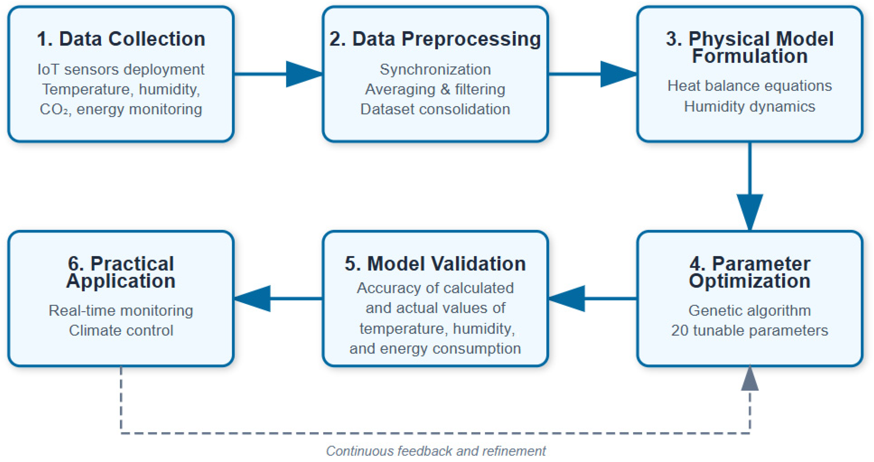
An overview of the complete modeling methodology is presented in Figure 2. This flowchart illustrates the six sequential stages of our approach: (1) data collection; (2) data preprocessing; (3) physical model formulation; (4) parameter optimization via genetic algorithm; (5) model validation; and (6) practical application, providing the reader with a clear roadmap before the detailed descriptions in Section 2.2, Section 2.3, Section 2.4, Section 3.1, Section 3.2 and Section 3.3.

2.2. Architecture of the Phytotron Microclimate Data-Acquisition System Using SenseCAP LoRaWAN

For the development of a temperature and humidity data-acquisition system, the following sensors and hardware were employed:
  • SenseCAP S2101-LoRaWAN® Air temperature and humidity sensor. A battery-powered, IP66-rated wireless air-temperature and humidity sensor with a measurement range of −40 °C to 85 °C and 0–100% RH. It features built-in Bluetooth and supports Over-the-Air configuration and remote management via a mobile app. Commonly used in Smart Farming, Smart Yard, and Smart City deployments.
  • SenseCAP S2103 LoRaWAN® CO2, temperature, and humidity sensor. A battery-powered, IP66-rated wireless sensor for CO2 (400–10,000 ppm), air temperature (−40 °C to 85 °C), and relative humidity (0–100%).
  • SenseCAP Outdoor gateway. The central LoRaWAN® gateway for the SenseCAP network, which aggregates data from multiple SenseCAP sensors and forwards it to the cloud platform via LTE or Ethernet. Designed for high reliability and performance in large-scale deployments, it employs mutual authentication and AES encryption across the network. The IP66-rated enclosure and extended operating temperature range make it suitable for industrial use. Internally, it combines a Cortex-A8 1 GHz processor with an SX1301 LoRa® concentrator chip. It supports EU868, US915, CN470, and other regional frequency plans at up to +27 dBm output power.
  • SenseCAP S2120 8-in-1 LoRaWAN Weather sensor. A compact weather station that measures air temperature, humidity, wind speed and direction, rainfall intensity, ambient light intensity, UV index, and barometric pressure. Suitable for horticulture, agriculture, meteorology, urban environmental monitoring, and other applications. Low maintenance is ensured by its ultra-low power consumption, reliable operation, and built-in Bluetooth for Over-the-Air configuration and remote management.
The LoRaWAN network follows a “star-of-stars” topology: end devices (sensors) transmit uplink packets to the nearest gateways, which then forward the data to the central Network Server. Devices transmit a radio packet and open two short receive windows for possible downlink responses. LoRaWAN supports multiple device classes (including the energy-efficient Class A) and various acknowledgment modes. Communications occur in license-exempt ISM bands (e.g., ~868 MHz in Europe, 915 MHz in the USA, ~920 MHz in Asia), with optional operation at 433 MHz or 2.4 GHz. All payloads are protected by AES encryption.
Device registration and network configuration are managed via the SenseCAP Portal and mobile app. To pair a sensor with a gateway, the user simply scans the device’s QR code or manually enters its DevEUI, AppEUI, and AppKey. The web portal provides real-time status monitoring of gateways and nodes, graphical data visualization, report generation, and data export. Once sensors are linked, they appear in the portal’s device list, where historical CSV downloads and trend analysis are available.
As a proof-of-concept, the current implementation uses SenseCAP sensors integrated with Home Assistant. For commercial-scale deployments, we recommend industrial-grade LoRaWAN gateways (e.g., MultiTech, Kerlink) with MQTT over TLS encryption and clustering support, alongside high-availability brokers, such as EMQX or VerneMQ and CI/CD pipelines, for automated firmware- and container-image updates. In addition, IT teams should establish clear zones of responsibility, implement role-based access control, conduct regular access audits, and maintain systematic data backup and recovery procedures.
This system architecture, featuring separation of the physical sensor layer and the cloud-based model layer, aligns with current best practices for digital twin development [42].

2.3. System for Energy Consumption Data Acquisition Using Smart-Home Sensors and Home Assistant

For the creation of the energy consumption data acquisition system, the following sensors and hardware were used:
  • Tuya smart plugs into which the dehumidifier, convector, and electric heater are connected. These plugs include built-in power-measurement sensors.
  • Taxnele TVPS1-63FW multifunction smart voltage relays (Yueqing Taixin Electric Co., Ltd., Yueqing, Zhejiang Province, China), inserted in the circuits of the air conditioner and the grow-light lamps.
  • Orange Pi 5 Ultra—a single-board computer (Shenzhen Xunlong Software Co., Ltd., Shenzhen, China) running Home Assistant software OS 11.0, which handles data collection and storage. The board is based on the Rockchip RK3588, featuring eight cores (four Cortex-A76 at 2.4 GHz and four Cortex-A55 at 1.8 GHz) and 64 GB of eMMC storage. This configuration delivers high performance and sufficient network throughput for the task. Home Assistant is deployed via Docker on the Orange Pi, which ingests data from the smart plugs and relays and stores it locally; no cloud services are used.
The smart plugs and relays join the local Wi-Fi network. Device onboarding is performed with the Smart Life mobile app. Each device is linked to the user’s Tuya account and, via the Tuya Developer platform and its API, integrated into Home Assistant.
Home Assistant is an open-source home-automation platform that serves as the central hub for collecting, storing, and analyzing IoT device data. It unifies the Wi-Fi plugs and smart relays into a single interface with customizable dashboards. Users can create pages composed of cards displaying real-time sensor readings (temperature, humidity, power, etc.) and plot time-series graphs. This makes it easy to monitor energy consumption (e.g., rendering individual power profiles for each plug or relay).
All sensor values in Home Assistant are persisted to a local SQLite database. Historical data can be queried to generate reports or exported for incorporation into the digital-twin model.

2.4. Data Analysis and Software Development Approach

Data analysis and the construction of consolidated datasets for the microclimate and energy-consumption monitoring system were carried out using Python 3.14 with the pandas, NumPy, and matplotlib libraries.
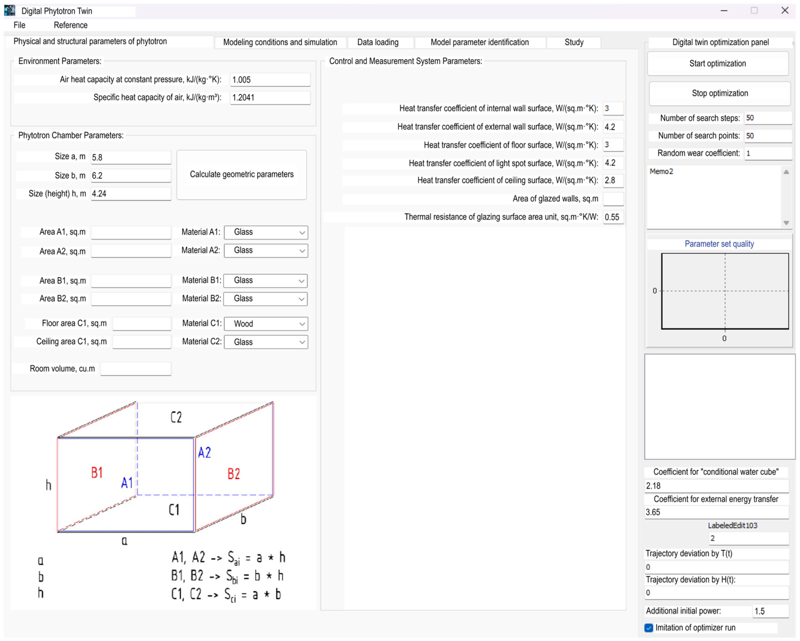
The Windows application “Phytotron Digital Twin” was developed in Embarcadero RAD Studio XE8 using C++ 03.

3. Results and Discussion

3.1. Object of Modeling

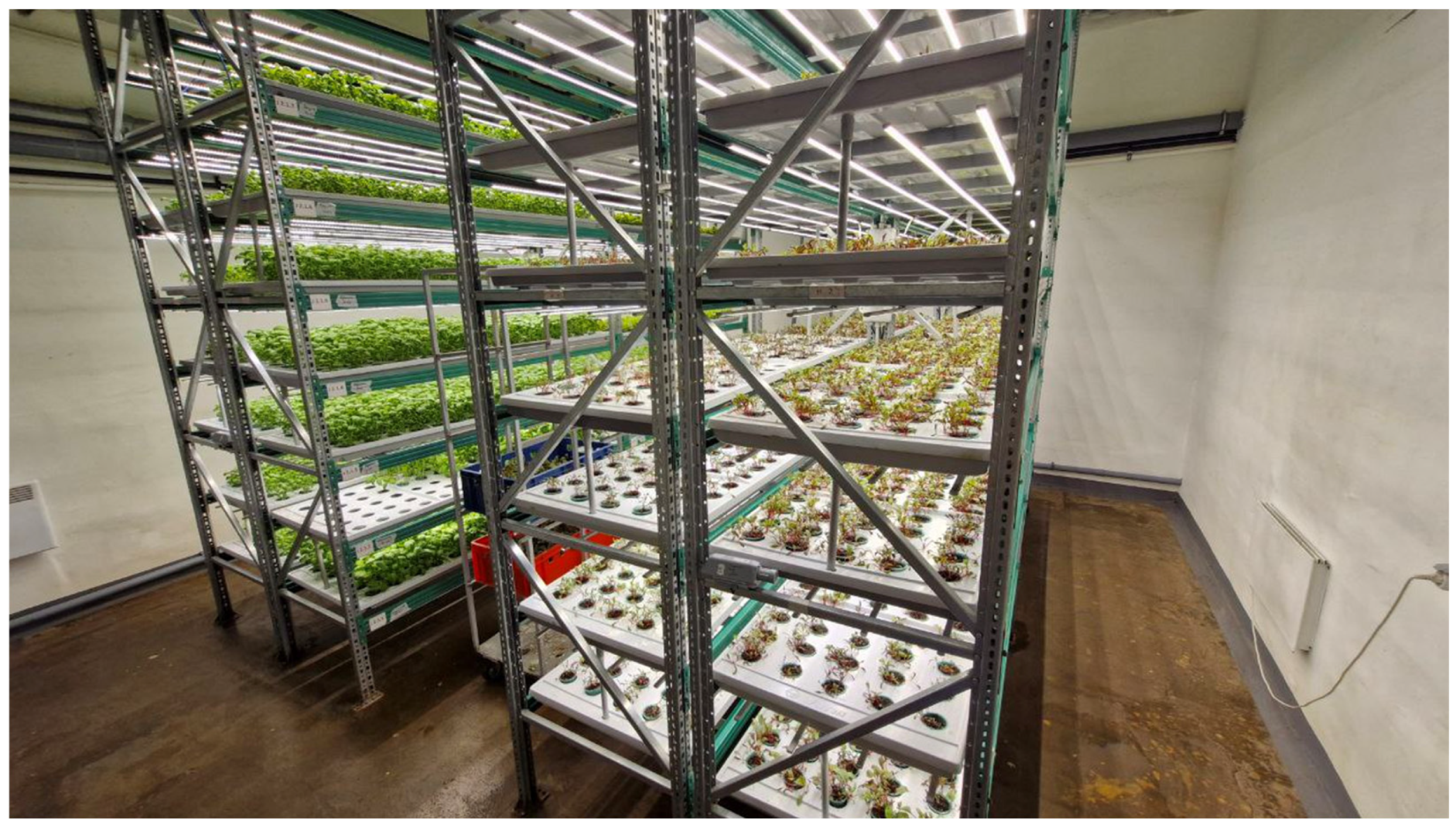
The object of modeling is the phytotron—a chamber measuring 5800 × 6200 × 4240 mm, dedicated to the cultivation of a single crop (basil). The phytotron is situated in a corner basement room. Two of its walls are 600 mm thick brick foundation walls backed by soil; one partition wall is 120 mm thick brick, and the opposite partition is 100 mm thick foam board. The ceiling consists of 100 mm thick ribbed slabs, and the floor is made of 220 mm thick reinforced-concrete panels. A photograph of the room is shown in Figure 3.
It is worth noting that the two seven-tier racks were installed by the site contractor, and their placement was not determined by the authors. During construction, the equipment and crop supplier provided recommendations on the optimal spatial arrangement of the racks, instruments, and sensors to ensure uniform airflow and favorable plant growth.
The vertical city farm occupies two shelving units, each with seven shelf levels. Every level accommodates 640 planting sites, for a total of 4480 positions. Each shelf is lit by LED fixtures, with a combined lighting load of 6480 W. The lights operate for 16 h per day.
At the time of study, the phytotron was an active testbed performing concurrent cultivar trials. As a result, plants on different shelves varied in age. This mosaic of developmental stages reflects typical research-scale operations; larger production farms would zone by crop age. Assessment of the model’s sensitivity to varying biomass loads, however, is beyond the scope of the present work and will be addressed in subsequent studies.
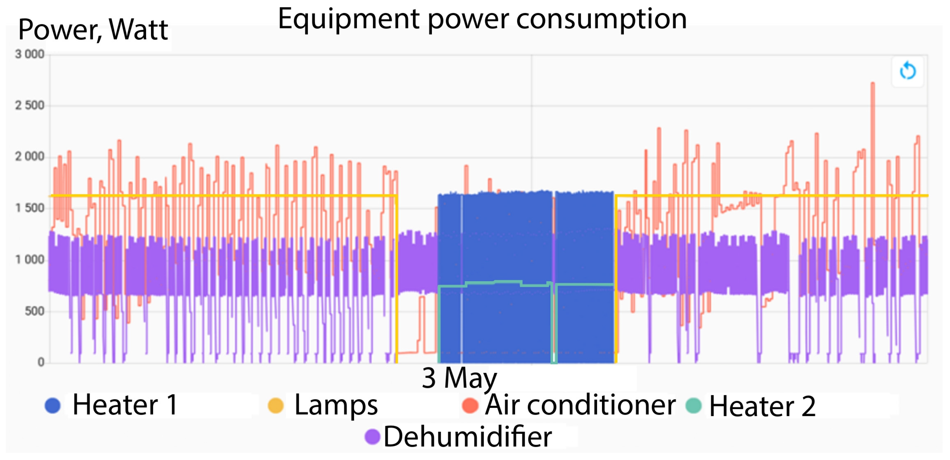
Microclimate control is provided by an inverter air-conditioning unit consuming 3.4 kW, with a cooling capacity of 10.9 kW and a heating capacity of 11.3 kW; it runs in automatic mode to maintain the programmed temperature setpoints. Humidity is regulated by two dehumidifiers with a total power draw of 1040 W. During the nighttime lighting-off period, electric heaters with a combined power of 2200 W are activated to sustain the required temperature.

3.2. Monitoring System

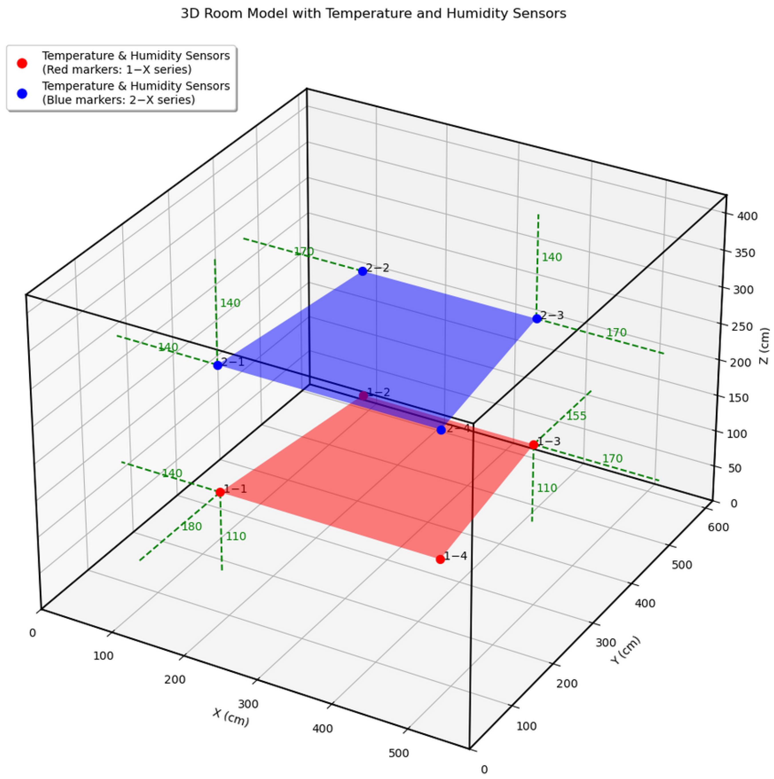
The arrangement of temperature and humidity sensors is shown in Figure 4.
This arrangement of sensors was chosen for uniform distribution throughout the room, taking into account their number. For ease of installation and quick access, as well as to limit the influence of lighting fixtures on temperature readings, the sensors are mainly located on the stand. Since the automation system and digital twin rely on the average value of indicators throughout the room, the issue of the influence of plant mass and illumination at individual points was not considered but is planned for study when moving to modeling macro- and microzones.
Because the chamber is fully enclosed and relies exclusively on LED fixtures, external solar effects (sunrise and sunset) on light intensity and spectral composition are effectively zero. In practice, light intensity remains constant throughout each 16 h photoperiod, simplifying model inputs and obviating the need to simulate natural dawn/dusk transitions.
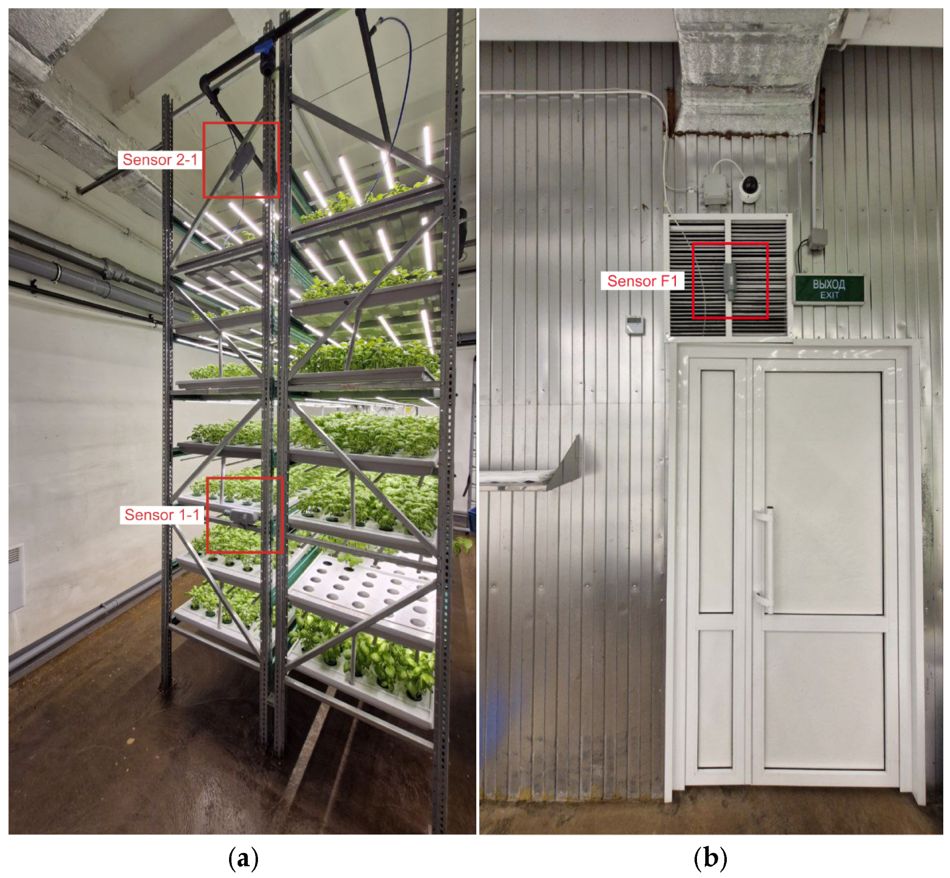
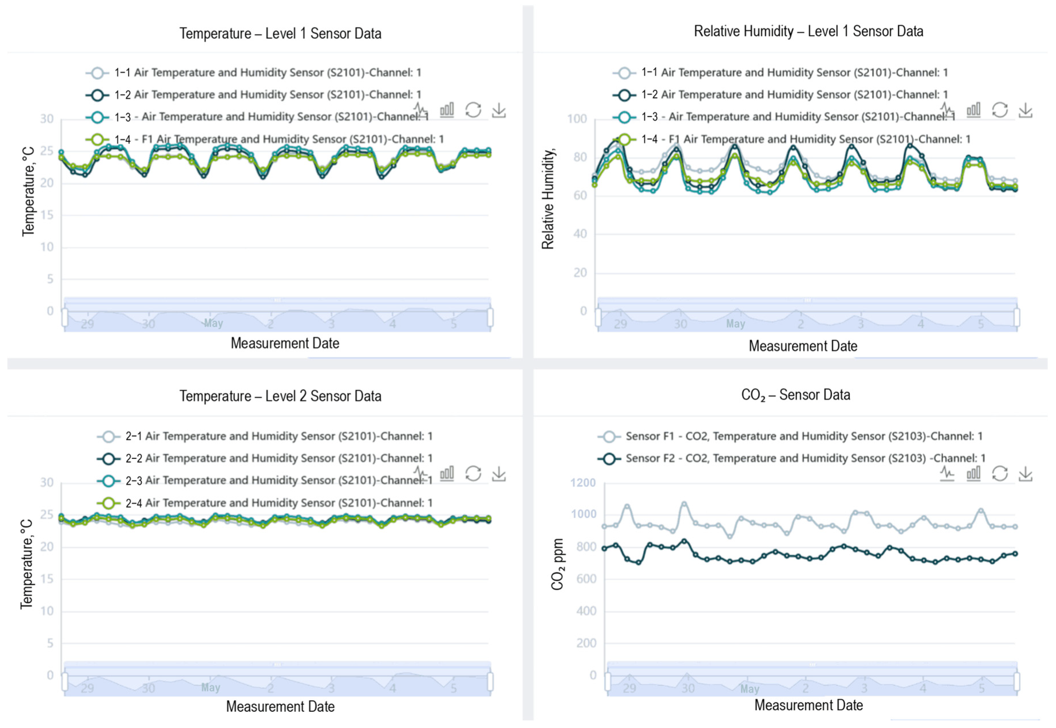
CO2 sensors are installed at the room’s ventilation grille (Sensor F1) and in the adjacent corridor space (Sensor F2). The placement of selected sensors is illustrated in Figure 5.
The position of sensor 1–3, located close to the plant canopy, is shown in Figure 5a. Sensor 1–2 is located symmetrically to it on another rack. And the second-level sensors marked 2–2 and 2–3 are located in the same plane as 2–1 and 2–4 and are fastened to the frame above the last level of plant illumination, as shown in Figure 6b.
The microclimate monitoring data are exported to the manufacturer’s database; the SenseCAP dashboard web interface is shown in Figure 7.
A review of the dynamics of the indoor CO2 content shows that the stable value for several weeks is 900–1100 ppm and does not go beyond the range. This confirms the hypothesis put forward in the methodology section about the insignificant mixing of CO2 due to human presence and the stable operation of the automated CO2 injection system.
The graphical representation of energy-consumption monitoring data on the Home Assistant platform is presented in Figure 8.
Part of the consolidated dataset is shown in Figure 9.

3.3. Analysis of Collected Data and Validation of the Computational Model

Figure 10 shows the main window interface of the developed software, which allows setting the initial physical and structural parameters of the phytotron and its environment.
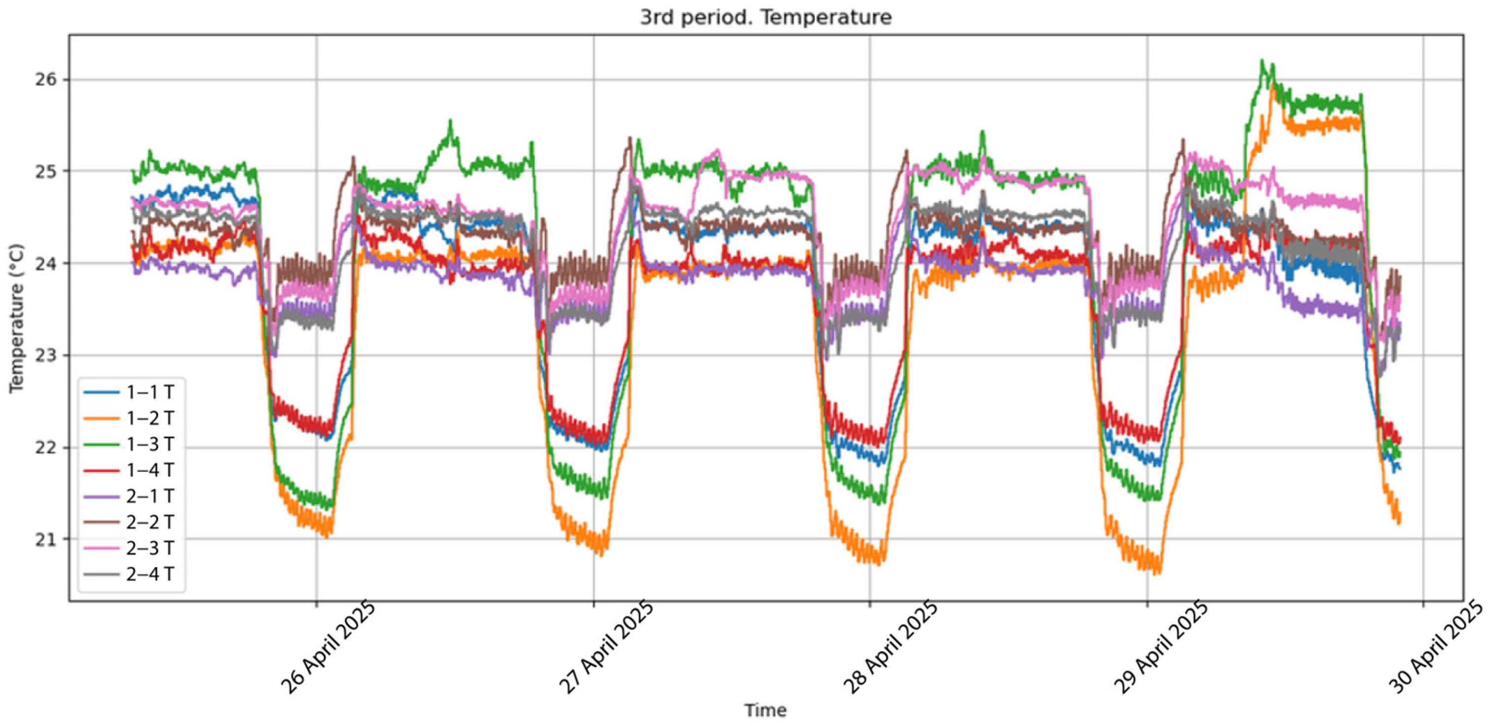
Complete datasets from the microclimate and energy-consumption monitoring systems were collected over three intervals: 72 h (10–13 April 2025), 90 h (14–18 April 2025), and 110 h (25–29 April 2025).
Initially, the selected intervals were tied to daily cycles and were 3, 4, and 5 days of one spring season. However, due to several power outages at the facility, such truncated intervals with high-quality data were determined to test the selected hybrid approach and build and refine the model.
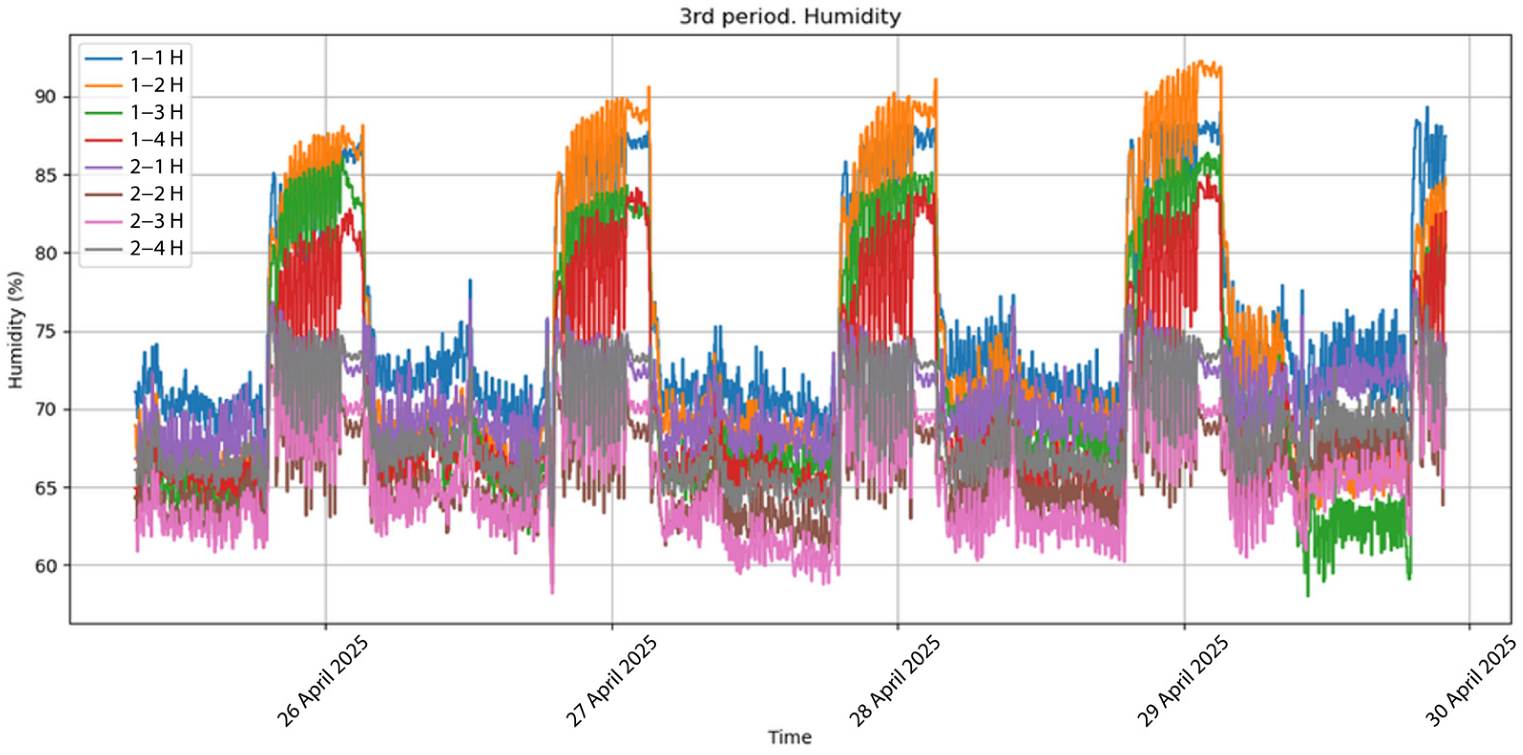
Temperature and humidity values from all the sensors are shown in Figure 11 and Figure 12.
It can be observed that temperature and humidity readings in different zones of the chamber differ substantially. Temperature values across sensors vary by 1–3 °C, and humidity by 15–30%. The differences are especially pronounced at night, when the artificial lighting system is turned off. This indicates microclimate heterogeneity within the phytotron, varying thermal conditions, and possibly poor air circulation due to suboptimal equipment placement.
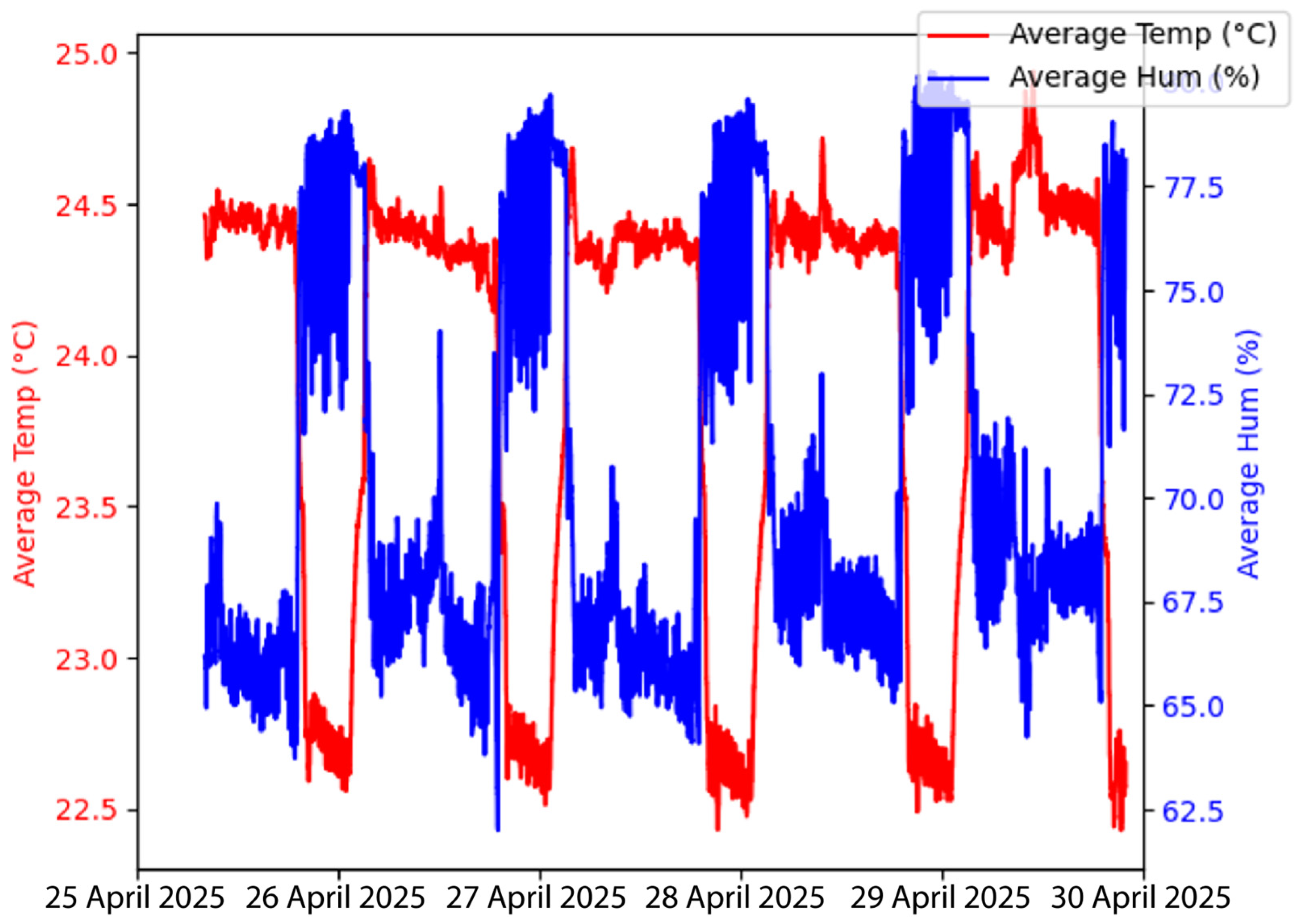
Nevertheless, the overall trends in the readings are consistent across all the sensors. For validation of the computational model against the monitoring data, averaged temperature and humidity values were used (Figure 13), since the automated microclimate control system operates on averaged inputs.
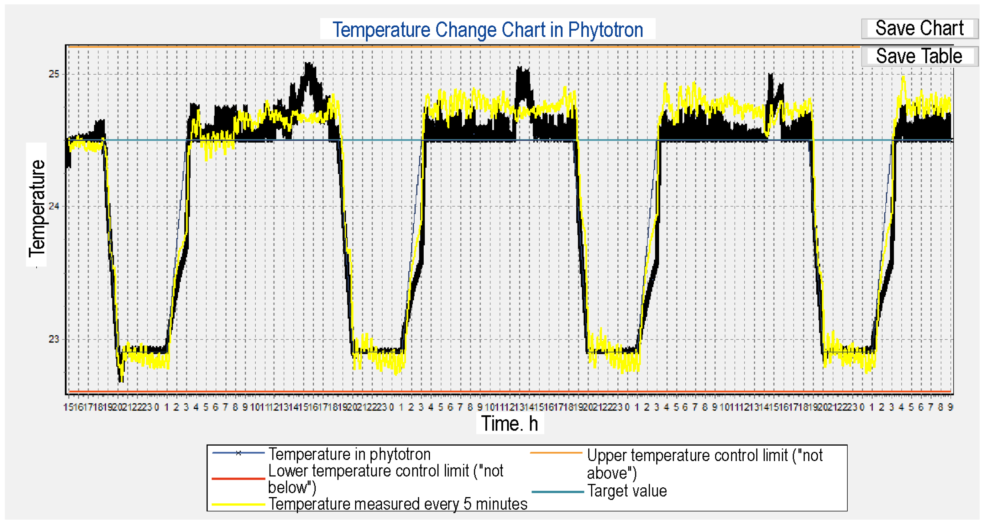
Power consumption data from the phytotron’s climate control devices, along with the temperature and humidity sensor readings, were imported into the simulation software. To ensure convergence of the computational model with the monitoring data, optimization was performed using a genetic algorithm, a population-based metaheuristic that iteratively evolves a set of candidate solutions through selection, crossover, and mutation operations over the 20 parameters described in Section 2.1. The resulting temperature profile for the first 72 h interval is shown in Figure 14.
Black denotes the simulated temperature values in the phytotron, and yellow denotes the actual measurements. The general patterns of temperature rise and fall in the computational model closely reproduce the real system behavior. The temperature profile for the second 90 h interval is presented in Figure 15.
A series of optimization experiments was carried out to identify a stable solution. A comparison of mean deviations for the best-performing parameter sets is given in Table 1.
A comparison of computed versus actual energy consumption over the three time intervals is given in Table 2.
The optimized computational model predicts the total accumulated energy consumption of the system with high fidelity—99.5% accuracy—while achieving mean temperature deviations of 0.1 °C and relative humidity deviations of approximately 2%.
The primary concept and original goal of the virtual system was to accurately describe the real processes occurring within the existing physical facility, a target which has now been achieved. The digital twin models temperature dynamics with a resolution of ±0.1 °C. Although individual sensor readings may deviate by up to 1.5 °C due to localized hot and cold spots—as noted by the reviewer—these variations do not compromise the model’s effectiveness for the studied vertical farm. To address such spatial heterogeneity and ensure reliable averaging both system-wide and within local zones, we propose installing forced-ventilation ducts at strategic points on each level, which will homogenize the identified fluctuations.
In addition to active solutions, such as forced-ventilation ducts, passive homogenization techniques are also applied in practice. Specifically, several manufacturers employ perforated or lattice inlet surfaces that diffuse the incoming airflow before it enters the chamber, thereby reducing spatial gradients of temperature and humidity. Although such solutions were not implemented in the present study, they represent a proven engineering approach that can complement digital-twin-based control strategies.
It should be noted that the genetic algorithm optimization performed over the three relatively short intervals (72–110 h) provides only a “snapshot” tuning of model parameters. To capture seasonal variations and equipment wear, we recommend re-optimizing over a longer time series (at least 1–3 months) and incorporating stability criteria into the objective function (for example, compressor smoothness or minimization of on/off cycling amplitudes).

3.4. Model Generalizability and Adaptation

The proposed digital twin framework was developed and validated for a basil phytotron. The following adaptations are possible to improve the model’s versatility:
  • The transpiration model (Equation (9)) can be adapted for different crops by varying the values of Itransp, Atransp, and Lcycle based on species-specific physiological data.
  • The model’s heat balance Equations (1)–(3) scale linearly with room volume and surface area, making them applicable to a variety of facilities, from small research chambers to commercial-scale vertical farms.
  • The outside temperature model (Equation (10)) can incorporate regional climate data, with the tdelay value adjusted based on local building thermal mass characteristics.
  • The energy models (Equations (11)–(15)) use common power ratings and efficiency factors, allowing for substitution of different HVAC systems, lighting technologies, and dehumidification equipment.

3.5. Economic Analysis

The initial cost to build such a monitoring system includes the following:
  • LoRaWAN sensors (8 × S2101 + 1 × S2103): ~USD 1200;
  • Gateway and weather station: ~USD 800;
  • Smart plugs and meters: ~USD400;
  • Orange Pi 5 and software development: ~USD 500.
  • Total initial cost: ~USD 2900
At this stage, our digital twin demonstrates the capabilities of high-precision monitoring and modeling. The economic benefit will be determined only after the implementation and validation of optimization algorithms in future work.
The cost of implementing the monitoring system (~USD 2900) represents the minimum investment required to build the digital twin infrastructure. This lays the foundation for future optimization efforts. Future work will focus on developing and testing optimization algorithms for the following:
  • Dynamically adjusting the temperature setpoint depending on the growth stage of plants;
  • Predictive control to minimize the cycling of HVAC systems;
  • Optimizing the LED spectrum depending on environmental conditions.
Only after implementing and testing these algorithms will it be possible to quantify the real economic benefits.

3.6. Comparison with Existing Microclimate Control Approaches

Modern digital twin models show a root mean square error of temperature forecasting below 1.3 °C in tests [43]. When validating CFD models around 1 °C [44], neural network approaches show accuracy at the level of RMSE = 0.787 °C [45] for temperature and 0.62% for humidity [46].
The results of our economic policy, however, have several advantages:
  • Ensure the accuracy of the calculation optimization parameters at first;
  • Computational requirements are reduced compared to CFD or ML methods;
  • Practical cost is reduced due to the use of commercial Internet sensors;
  • Adaptability, at first, is possible to take into account the optimization of genetic algorithms.
Unlike CFD models, which require extensive computing resources and detailed 3D geometry, our approach provides increased accuracy with standard computing equipment. Compared to a pure machine learning approach, our physics-based framework provides stable interpretability and requires less training data.

3.7. Future Work

Future work will focus on the following directions:
  • Developing mechanisms for remote firmware updates of sensors and controllers and for automated database aggregation;
  • Introducing predictive modeling based on machine learning to forecast microclimate parameters and plant-growth dynamics [47];
  • Reducing overall energy consumption via adaptive control of LED lighting, air conditioning, and dehumidification based on analytical predictors. Shifting from static setpoints to dynamic profiles will improve system efficiency without compromising yield [48];
  • Implementing an additional control loop to ensure real-time operation with feedback on environmental quality;
  • Investigating the integration of computer-vision and image-processing technologies for automatic plant-health monitoring or verification of personnel operations;
  • Applying nonparametric system identification methods to achieve more accurate approximation of system characteristics, even in the absence of detailed initial-state information, thereby simplifying model validation and improving model quality;
  • Optimizing production from a business-process perspective. Resource allocation strategies that maximize satisfaction of multiple product consumer demands will require long-term production planning (over months or years) and agile adaptation to changing market conditions [49];
  • Developing and testing resilience mechanisms: periodic sensor calibration, LoRaWAN packet loss monitoring, and channel redundancy, as well as a strategy for automatic switching to backup controllers in the event of a node outage;
  • Extending the current single-zone model to a spatially resolved digital twin—initially via a simple 2 × 2 grid of zones and subsequently through CFD-based approximations—to capture shelf- and row-level microclimatic variations and improve local control fidelity;
  • Investigating the comparative effectiveness of passive homogenization methods (e.g., perforated or lattice inlet surfaces) versus active ventilation strategies. A systematic evaluation of these approaches in terms of airflow uniformity, energy efficiency, and cost will provide further guidance for practical deployment in large-scale vertical farming facilities;
  • Expanding calibration periods to cover longer datasets (minimum 1–3 months) and introduce multi-objective optimization that balances energy efficiency with equipment longevity and minimizes negative control pulsations (e.g., amplitude of compressor switching cycles).

4. Conclusions

This study has successfully developed and validated a digital-twin framework for a basil cultivation phytotron using a hybrid approach that couples a physico-mathematical microclimate model with an IoT-based monitoring system.
The main results of the research include the following:
  • Development of a microclimate model. A comprehensive system of heat-balance, humidity, and energy-consumption equations was formulated, accounting for all climate-control systems and plant transpiration.
  • Implementation of a distributed monitoring system. A scalable IoT architecture based on LoRaWAN and Wi-Fi technologies was deployed, enabling data collection for temperature, humidity, CO2, and equipment power use.
  • Hybrid model validation. A genetic algorithm (GA)—an evolutionary optimization method—was employed to optimize the model parameters against real monitoring data, achieving high predictive accuracy (0.1 °C temperature deviation, 2% humidity deviation).
  • Verification of energy-efficiency predictions. The optimized model predicted total energy consumption with 99.5% accuracy, confirming its suitability for resource-usage optimization.
The proposed framework offers significant potential for real-world application in vertical-farm and controlled-environment agriculture control systems, enabling precise microclimate regulation and optimal energy management.

Author Contributions

Conceptualization, V.V.B., Y.V.T. and I.A.T.; methodology, V.V.B., I.S.N., A.A.G. and S.I.L.; software, V.V.B., I.S.N. and S.A.K.; validation, V.V.B., I.S.N. and A.A.G.; formal analysis, I.S.N.; investigation, V.V.B., I.S.N. and A.A.G.; resources, I.S.N.; data curation, V.V.B. and I.S.N.; writing—original draft preparation, I.S.N.; writing—review and editing, V.V.B. and I.S.N.; visualization, V.V.B. and I.S.N.; supervision, V.V.B. and I.A.T.; project administration, V.V.B. and I.A.T.; funding acquisition, I.A.T. All authors have read and agreed to the published version of the manuscript.

Funding

This research was supported by the Ministry of Science and Higher Education of the Russian Federation (grant number 075-15-2024-682) for the project “Development and research of multi-tiered plant growing technology for traditional plant growing complexes using energy-efficient artificial LED phytolighting with digitalization of elements” and project of The Belarusian Republican Foundation for Fundamental Research №Φ23КУБ-006.

Conflicts of Interest

The authors declare no conflicts of interest.

Abbreviations

The following abbreviations are used in this manuscript:
IoTInternet of things
CFDComputational fluid dynamics
LoRaWANLong-range wide-area network
Wi-FiWireless fidelity
LEDLight-emitting diode
CO2Carbon dioxide
GPSGlobal positioning system
HAHome Assistant
ISMIndustrial, scientific, and medical (bands)
AESAdvanced encryption standard
DTDigital twin
NB-IoTNarrowband Internet of Things
RMSERoot mean square error
GAGenetic algorithm

References

  1. Zhang, R.; Zhu, H.; Chang, Q.; Mao, Q. A Comprehensive Review of Digital Twins Technology in Agriculture. Agriculture 2025, 15, 903. [Google Scholar] [CrossRef]
  2. Rathor, A.S.; Choudhury, S.; Sharma, A.; Nautiyal, P.; Shah, G. Empowering vertical farming through IoT and AI-Driven technologies: A comprehensive review. Heliyon 2024, 10, 34998. [Google Scholar] [CrossRef]
  3. Costa, G.P.; Sakata, G.Y.A.; Oliveira, L.F.P.D.; Chaves, M.E.; Duarte, L.F.; Matulovic, M.; Buzo, R.F.; Morais, F.J. FarmSync: Ecosystem for Environmental Monitoring of Barns in Agribusiness. AgriEngineering 2025, 7, 124. [Google Scholar] [CrossRef]
  4. Stamford, J.D.; Stevens, J.; Mullineaux, P.M.; Lawson, T. LED lighting: A grower’s guide to light spectra. HortScience 2023, 58, 180–196. [Google Scholar] [CrossRef]
  5. Pereira, J.; Gomes, M.G. Lighting strategies in vertical urban farming for enhancement of plant productivity and energy consumption. Appl. Energy 2025, 377, 124669. [Google Scholar] [CrossRef]
  6. Rahman, H.; Shah, U.M.; Riaz, S.M.; Kifayat, K.; Moqurrab, S.A.; Yoo, J. Digital twin framework for smart greenhouse management using next-gen mobile networks and machine learning. Future Gener. Comput. Syst. 2024, 156, 285–300. [Google Scholar] [CrossRef]
  7. Chaux, J.D.; Sanchez-Londono, D.; Barbieri, G. A digital twin architecture to optimize productivity within controlled environment agriculture. Appl. Sci. 2021, 11, 8875. [Google Scholar] [CrossRef]
  8. Monteiro, J.; Barata, J.; Veloso, M.; Veloso, L.; Nunes, J. A scalable digital twin for vertical farming. J. Ambient Intell. Humaniz. Comput. 2023, 14, 13981–13996. [Google Scholar] [CrossRef]
  9. Bersani, F.; Capra, A.; Rovai, M.; Francini, A.; Al-Sharmouri, N.; Orsini, F.; Gianquinto, G. Internet of Things approaches for monitoring and control of smart greenhouses in Industry 4.0. Energies 2022, 15, 3834. [Google Scholar] [CrossRef]
  10. Saad, M.H.M.; Hamdan, N.M.; Sarker, M.R. State of the art of urban smart vertical farming automation system: Advanced topologies, issues and recommendations. Electronics 2021, 10, 1422. [Google Scholar] [CrossRef]
  11. Farooq, M.S.; Riaz, S.; Abid, A.; Abid, K.; Naeem, M.A. A Survey on the Role of IoT in Agriculture for the Implementation of Smart Farming. IEEE Access 2019, 7, 156237–156271. [Google Scholar] [CrossRef]
  12. Ariesen-Verschuur, N.; Verdouw, C.; Tekinerdogan, B. Digital Twins in greenhouse horticulture: A review. Comput. Electron. Agric. 2022, 199, 107183. [Google Scholar] [CrossRef]
  13. Avşar, E.; Mowla, M.N. Wireless communication protocols in smart agriculture: A review on applications, challenges and future trends. Ad Hoc Netw. 2022, 136, 102982. [Google Scholar] [CrossRef]
  14. Singh, N.; Sharma, A.K.; Sarkar, I.; Prabhu, S.; Chadaga, K. IoT-based greenhouse technologies for enhanced crop production: A comprehensive study of monitoring, control, and communication techniques. Syst. Sci. Control. Eng. 2024, 12, 2306825. [Google Scholar] [CrossRef]
  15. Platero-Horcajadas, M.; Pardo-Pina, S.; Cámara-Zapata, J.M.; Brenes-Carranza, J.A.; Ferrández-Pastor, F.J. Enhancing Greenhouse Efficiency: Integrating IoT and Reinforcement Learning for Optimized Climate Control. Sensors 2024, 24, 8109. [Google Scholar] [CrossRef] [PubMed]
  16. Sowmya, C.; Anand, M.; Indu Rani, C.; Amuthaselvi, G.; Janaki, P. Recent developments and inventive approaches in vertical farming. Front. Sustain. Food Syst. 2024, 8, 1400787. [Google Scholar] [CrossRef]
  17. Escribà-Gelonch, M.; Liang, S.; van Schalkwyk, P.; Fisk, I.; Long, N.V.D.; Hessel, V. Digital twins in agriculture: Orchestration and applications. J. Agric. Food Chem. 2024, 72, 10737–10752. [Google Scholar] [CrossRef]
  18. Verdouw, C.; Beulens, A.; van der Voort, M.; Verloop, C.; Tromp, S. Digital twins in smart farming. Agric. Syst. 2020, 189, 103046. [Google Scholar] [CrossRef]
  19. Conti, Z.X.; Ward, R.; Choudhary, R. Energy Modelling and Forecasting for an Underground Agricultural Farm using a Higher Order Dynamic Mode Decomposition Approach. arXiv 2023, arXiv:2306.15089. [Google Scholar] [CrossRef]
  20. Nasirahmadi, S.; Hensel, O. Toward the next generation of digitalization in agriculture based on digital twin paradigm: A comprehensive review. Sensors 2022, 22, 498. [Google Scholar] [CrossRef]
  21. Shrivastava, A.; Nayak, C.K.; Dilip, R.; Samal, S.R.; Rout, S.; Ashfaque, S.M. Automatic robotic system design and development for vertical hydroponic farming using IoT and big data analysis. Mater. Today Proc. 2023, 80, 3546–3553. [Google Scholar] [CrossRef]
  22. Morella, P.; Lambán, M.P.; Royo, J.; Sánchez, J.C. Vertical Farming Monitoring: How Does It Work and How Much Does It Cost? Sensors 2023, 23, 3502. [Google Scholar] [CrossRef] [PubMed]
  23. Peladarinos, N.; Piromalis, D.D.; Cheimaras, V.; Tserepas, E.; Munteanu, A.; Papageorgas, P. Enhancing Smart Agriculture by Implementing Digital Twins: A Comprehensive Review. Sensors 2023, 23, 7128. [Google Scholar] [CrossRef] [PubMed]
  24. Purcell, W.; Neubauer, T. Digital Twins in Agriculture: A State-of-the-art review. Smart Agric. Technol. 2023, 3, 100094. [Google Scholar] [CrossRef]
  25. Slob, N.; Hurst, W. Digital Twins and Industry 4.0 Technologies for Agricultural Greenhouses. Smart Cities 2022, 5, 1179–1192. [Google Scholar] [CrossRef]
  26. Kalyani, Y.; Vorster, L.; Whetton, R.; Collier, R. Application scenarios of digital twins for smart crop farming through cloud–fog–edge infrastructure. Future Internet 2024, 16, 100. [Google Scholar] [CrossRef]
  27. Bournet, P.E.; Rojano, F. Advances of Computational Fluid Dynamics (CFD) applications in agricultural building modelling: Research, applications and challenges. Comput. Electron. Agric. 2022, 201, 107277. [Google Scholar] [CrossRef]
  28. Sezer, N.; Yoonus, H.; Zhan, D.; Wang, L.L.; Hassan, I.G.; Rahman, M.A. Urban microclimate and building energy models: A review of the latest progress in coupling strategies. Renew. Sustain. Energy Rev. 2023, 184, 113577. [Google Scholar] [CrossRef]
  29. Mirzaei, P.A. CFD modeling of micro and urban climates: Problems to be solved in the new decade. Sustain. Cities Soc. 2021, 69, 102839. [Google Scholar] [CrossRef]
  30. Singh, M.C.; Yousuf, A.; Singh, J.P. Greenhouse microclimate modeling under cropped conditions-A review. Res. Environ. Life Sci. 2016, 9, 1552–1557. [Google Scholar]
  31. Kang, L.; Zhang, Y.; Kacira, M.; van Hooff, T. CFD simulation of air distributions in a small multi-layer vertical farm: Impact of computational and physical parameters. Biosyst. Eng. 2024, 243, 148–174. [Google Scholar] [CrossRef]
  32. Zhang, Y.; Kacira, M. Analysis of climate uniformity in indoor plant factory system with computational fluid dynamics (CFD). Biosyst. Eng. 2022, 220, 73–86. [Google Scholar] [CrossRef]
  33. Zhang, Y.; Kacira, M.; An, L. A CFD study on improving air flow uniformity in indoor plant factory system. Biosyst. Eng. 2016, 147, 193–205. [Google Scholar] [CrossRef]
  34. Plas, W.; De Paepe, M. Using CFD to improve flow conditions in vertical farms using realistic plant geometries. In Acta Horticulturae 1369, Proceedings of the XXXI International Horticultural Congress (IHC2022): International Symposium on Advances in Vertical Farming, Angers, France, 14–20 August 2022; International Society for Horticultural Science (ISHS): Leuven, Belgium, 2022; Volume 1369, pp. 49–56. [Google Scholar]
  35. Pylianidis, C.; Osinga, S.; Athanasiadis, I.N. Introducing digital twins to agriculture. Comput. Electron. Agric. 2021, 184, 105942. [Google Scholar] [CrossRef]
  36. Lin, Y.; Huang, T.; Yang, W.; Hu, X.; Li, C. A review on the impact of outdoor environment on indoor thermal environment. Buildings 2023, 13, 2600. [Google Scholar] [CrossRef]
  37. Hou, Y.; Cao, B.; Zhu, Y.; Zhang, H.; Yang, L.; Duanmu, L.; Lian, Z.; Zhang, Y.; Zhai, Y.; Wang, Z.; et al. Temporal and spatial heterogeneity of indoor and outdoor temperatures and their relationship with thermal sensation from a global perspective. Environ. Int. 2023, 179, 108174. [Google Scholar] [CrossRef]
  38. World Meteorological Organization (WMO). Guide to Instruments and Methods of Observation; (WMO-No. 8); WMO: Geneva, Switzerland, 2021. [Google Scholar]
  39. Dayer, S.; Herrera, J.C.; Dai, Z.; Burlett, R.; Lamarque, L.J.; Delzon, S.; Bortolami, G.; Cochard, H.; Gambetta, G.A. The sequence and thresholds of leaf hydraulic traits underlying grapevine varietal differences in drought tolerance. J. Exp. Bot. 2020, 71, 4333–4344. [Google Scholar] [CrossRef]
  40. Játiva, P.P.; Soto, I.; Azurdia-Meza, C.A.; Sánchez, I.; Wang, R.; Kern, W. Hybrid Digital Twin Model for Greenhouse and Underground Environments. IEEE Access 2024, 12, 73906–73924. [Google Scholar] [CrossRef]
  41. Codeluppi, G.; Cilfone, A.; Davoli, L.; Ferrari, G. LoRaFarM: A LoRaWAN-Based Smart Farming Modular IoT Architecture. Sensors 2020, 20, 2028. [Google Scholar] [CrossRef]
  42. Tekinerdogan, B.; Verdouw, C. Systems architecture design pattern catalog for developing digital twins. Sensors 2020, 20, 5103. [Google Scholar] [CrossRef]
  43. Jans-Singh, M.; Leeming, K.; Choudhary, R.; Girolami, M. Digital twin of an urban-integrated hydroponic farm. Data-Centric Eng. 2020, 1, e20. [Google Scholar] [CrossRef]
  44. Zainali, S.; Qadir, O.; Parlak, S.C.; Lu, S.M.; Avelin, A.; Stridh, B.; Campana, P.E. Computational fluid dynamics modelling of microclimate for a vertical agrivoltaic system. Energy Nexus 2023, 9, 100173. [Google Scholar] [CrossRef]
  45. Ardabili, S.; Mosavi, A.; Mahmoudi, A.; Gundoshmian, T.M.; Nosratabadi, S.; Várkonyi-Kóczy, A.R. Modelling temperature variation of mushroom growing hall using artificial neural networks. In Engineering for Sustainable Future, Proceedings of the International Conference on Global Research and Education, Budapest, Hungary, Balatonfüred, Hungary, 4–7 September 2019; Springer International Publishing: Cham, Switzerland, 2020; pp. 33–45. [Google Scholar]
  46. Chen, S.; Liu, A.; Tang, F.; Hou, P.; Lu, Y.; Yuan, P. A Review of Environmental Control Strategies and Models for Modern Agricultural Greenhouses. Sensors 2025, 25, 1388. [Google Scholar] [CrossRef]
  47. Thwin, K.M.M.; Horanont, T.; Phatrapornnant, T. Machine-Learning Microclimate Forecasting for Adaptive Equipment Control via Web Integration in Open-Ventilated Greenhouses. AgriEngineering 2024, 6, 2845–2869. [Google Scholar] [CrossRef]
  48. Kaiser, E.; Kusuma, P.; Vialet-Chabrand, S.; Folta, K.; Liu, Y.; Poorter, H.; Woning, N.; Shrestha, S.; Ciarreta, A.; van Brenk, J.; et al. Vertical farming goes dynamic: Optimizing resource use efficiency, product quality, and energy costs. Front. Sci. 2024, 2, 1411259. [Google Scholar] [CrossRef]
  49. Luo, Y.; Ball, P. Adaptive production strategy in vertical farm digital twins with Q-learning algorithms. Sci. Rep. 2025, 15, 15129. [Google Scholar] [CrossRef]
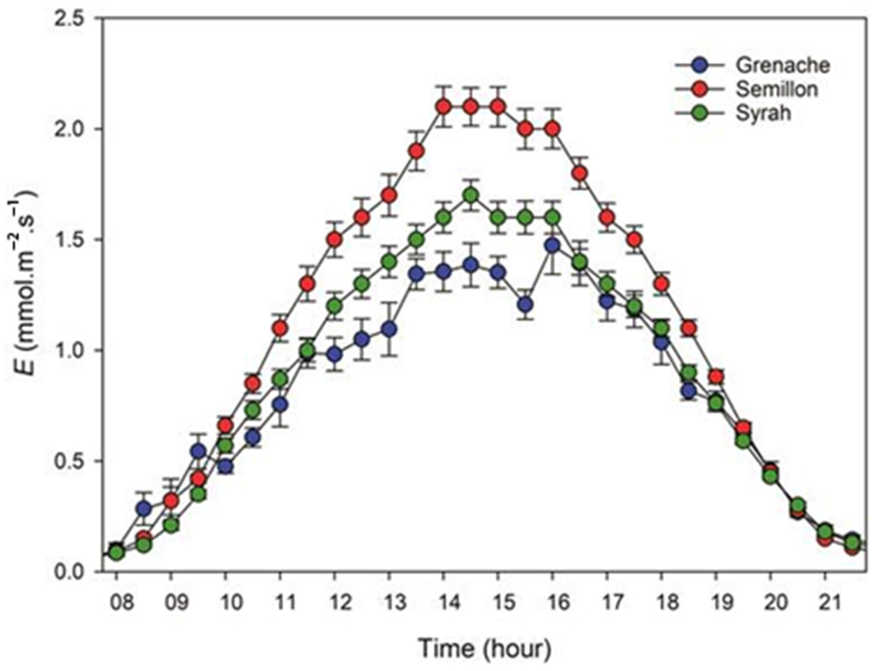
Figure 1. Daytime transpiration rate measured at the whole-plant scale and expressed per leaf area in well-watered plants of Grenache, Semillon, and Syrah. Each point is the hourly mean across 15 d of the experiment ±SE (n = 50–60) [39].
Agriengineering 07 00285 g001
Figure 2. A flowchart illustrating the modeling approach.
Agriengineering 07 00285 g002
Figure 3. Photo of shelving with basil plants.
Agriengineering 07 00285 g003
Figure 4. Layout diagram of phytotron temperature and humidity monitoring sensors.
Agriengineering 07 00285 g004
Figure 5. (a) Location of front-mounted temperature and humidity sensors; (b) CO2 sensor location.
Agriengineering 07 00285 g005
Figure 6. (a) The position of sensor 1-3, located close to the plant canopy; (b) position of sensors 2-3, located on the second level.
Agriengineering 07 00285 g006
Figure 7. Web interface of temperature and humidity monitoring system.
Agriengineering 07 00285 g007
Figure 8. Web interface of equipment power consumption monitoring system.
Agriengineering 07 00285 g008
Figure 9. Excerpt of the consolidated dataset with per-second power consumption values and microclimate sensor readings.
Agriengineering 07 00285 g009
Figure 10. Main interface of the “Phytotron Digital Twin” software (self-developed).
Agriengineering 07 00285 g010
Figure 11. Temperature readings from the phytotron microclimate monitoring system.
Agriengineering 07 00285 g011
Figure 12. Humidity readings from the phytotron microclimate monitoring system.
Agriengineering 07 00285 g012
Figure 13. Averaged temperature and humidity values for the third time interval.
Agriengineering 07 00285 g013
Figure 14. Temperature profile of the computational and monitoring models for the first interval.
Agriengineering 07 00285 g014
Figure 15. Temperature profile of the computational and monitoring models for the second interval.
Agriengineering 07 00285 g015
Table 1. Comparison of the computational model against monitoring system data.
Time IntervalMean Temperature Deviation, °CMean Humidity Deviation, %
First period (72 h)0.081.9
Second period (90 h)0.092.4
Third period (110 h)0.102.2
Table 2. Comparison of computed and actual system energy consumption.
Time IntervalCalculated Accumulated Energy Consumption (kWh)Actual Accumulated Energy Consumption (kWh)Relative Error, %
First period (72 h)474.3476.80.52
Second period (90 h)602.8601.20.26
Third period (110 h)748.7752.90.56
Disclaimer/Publisher’s Note: The statements, opinions and data contained in all publications are solely those of the individual author(s) and contributor(s) and not of MDPI and/or the editor(s). MDPI and/or the editor(s) disclaim responsibility for any injury to people or property resulting from any ideas, methods, instructions or products referred to in the content.