Article

Crop Identification with Monte Carlo Simulations and Rotation Models from Sentinel-2 Data

1
AI4AGRI, Romanian Excellence Center on AI for Agriculture, Transilvania University of Brasov, 500024 Brasov, Romania
2
Image Processing and Analysis Laboratory, National University of Science and Technology Politehnica Bucharest, Splaiul Independentei 313, 060042 Bucharest, Romania
*
Author to whom correspondence should be addressed.
AgriEngineering 2025, 7(8), 259; https://doi.org/10.3390/agriengineering7080259
Submission received: 23 June 2025 / Revised: 31 July 2025 / Accepted: 4 August 2025 / Published: 11 August 2025

Abstract

Crop rotation is a well-established practice that helps reduce nutrient depletion and pressure from pests and weeds. At the same time, the use of artificial intelligence tools to recognize crops from satellite multispectral imagery is gaining momentum as a first step toward automated agricultural monitoring. However, the recognition process is limited by inherent errors and the scarcity of available data. In this paper, we build upon Monte Carlo simulation methods to investigate whether incorporating crop rotation information—encoded as a Markov chain—can improve identification accuracy. To broaden the simulation across diverse datasets, we also synthesize multispectral pixels for underrepresented crop types. Crop rotation is used not only in post-processing, but also integrated into the classifier, where a Gradient Boosting Machine is adapted to penalize learners that predict the same crop as in the previous year. Our evaluation uses Sentinel satellite imagery of agricultural crops, combined with the DACIA5 database from the Brașov region of Romania. We conclude that incorporating accurate prior information and crop rotation models noticeably improves crop identification performance. Synthesized data further enhances recognition rates and enables broader applicability, beyond the original region.

1. Introduction

As human societies evolve and their needs become increasingly complex, the fundamental necessity for food remains unchanged. Rising demand, climate change, and sustainability challenges make it essential to use advanced technologies to boost crop yields with minimal environmental impact. Artificial intelligence (AI), when combined with remote sensing data, strengthens agricultural planning by identifying patterns, forecasting outcomes, and optimizing decision making for improved resource allocation and productivity [1]. Remote sensing (RS) has emerged as one of the most transformative tools in modern precision agriculture, enabling real-time monitoring, analysis, and prediction of vegetation health and land-use changes over vast geographic areas [2]. In parallel with these technological advancements, traditional practices such as crop rotation continue to play a vital role in maintaining soil fertility and improving long-term agricultural yields. Together, these innovations and practices are reshaping the future of sustainable agriculture.
Accurate and consistent crop mapping is essential for understanding and assessing the environmental impacts of agriculture, as well as for developing effective mitigation strategies. These maps are typically generated using a combination of remote sensing data, spatial reference information—such as Land Parcel Identification Systems (LPIS)—and, often, supplemented with field or environmental data. Notable examples are China’s CropWatch [3] and the U.S. Cropland Data Layer [4]. In countries such as France, Belgium, and the Netherlands, national LPIS datasets are openly accessible and have been compiled and standardized through the EuroCrops initiative [5].
Outside these official national datasets, large-scale crop maps have also been developed, often aimed at improving mapping methodologies or providing coverage in regions where official maps are lacking [6,7]. However, this process does not function uniformly across all regions. In some countries, detailed data are available only for small, localized areas, while for the broader regions (e.g., national level), only aggregated statistics are accessible.
For such mapping processes, two types of information are essential: accurate crop parcel annotations for the current year and historical data on previous crops. These two types of information are complementary, and their integration enables the development of automatic crop mapping systems.
In Romania, annual crop information is available only for limited parcels, such as those included in the DACIA5 dataset [8]. This dataset contains Sentinel-2 data spanning five years (2020–2024) for parcels managed by the National Institute of Research and Development for Potato and Sugar Beet (INCDCSZ), located just north of Brașov, Romania.
Meanwhile, the National Ministry of Agriculture publishes annual reports on land use and crop yields at the national level. Since parcel annotation is costly and time-consuming, there is growing interest in deploying models trained on existing annotated datasets. In this paper, we first use Monte Carlo simulations to extrapolate data from small, localized areas to align with national-level statistics. Second, using this more robust and representative set of crop samples, we simulate various crop rotation models with similar techniques. The rotation model is also integrated into the classifier, which is adapted to penalize learners that predict the same crop as in the previous year. All these components are combined, and comparative evaluations are conducted to assess performance improvements.
The remainder of the paper is organized as follows. In the next subsection, we review relevant prior work. Section 2 presents the original database, followed by a description of the methods used to synthesize new pixels, incorporate actual crop rotation data, and apply the rotation model within classifiers. Section 3 covers the evaluation. First, it analyzes how well the synthesized data matches the real data. Then, it addresses the problem of crop identification, evaluating the impact of different rotation patterns on recognition performance and how the solution adapts to varying crop distributions. The paper concludes with discussions and final remarks.

1.1. Prior Work

From a technical standpoint, this paper aims to contribute to a better understanding of the role of crop rotation in crop identification from satellite imagery, and to provide a method for synthesizing data similar to existing datasets, thereby enhancing the generalizability of the proposed solution.

1.1.1. Crop Identification Using Rotation Models

Crop rotation is a well-known and widely applied principle in agriculture. Due to its widespread adoption, it has influenced automated agricultural data analysis. For instance, Wang et al. [9] enhanced Random-Forest-based crop identification by incorporating spatial heterogeneity derived from crop rotation principles—specifically, they examined changes in crop templates relative to the previous year. Crop rotation is designed to prevent the depletion of soil nutrients, and Yang et al. [10] used Fourier decomposition to monitor this process over multiple years. Giordano et al. [11] modeled crop rotation patterns using a Markov model, followed by Random Forest classification on Sentinel-2 data from two localized study areas in France.
Recently, deep learning models have increasingly been used for crop classification, either based on time series or image patches. Crop rotation models have been integrated into deep learning analyses of time series data for parcels, as demonstrated by Quinton et al. [12], who injected rotation information into the decision-making blocks of their model.
A large dataset enabling a more thorough investigation of crop rotation implementation in England was analyzed by Upcott et al. [13], while a similar study focused on China was conducted by Liu et al. [14]. The effects of crop rotation on soil microorganisms have also been extensively studied [15], and the environmental impact of specific crops has also been investigated [16].
Although large farms have traditionally been the focus, recent research has also addressed crop rotation patterns in small farms [17]. Additionally, crop rotation data has been combined with satellite and contextual data for improved analysis [18].
However, we note that while prior work has successfully incorporated crop rotation information into the prediction of current crop distributions, most models have been limited to existing, localized data without extrapolating to broader statistical patterns. Our paper aims to address this gap.

1.1.2. Monte Carlo Simulation in Agriculture Data

The challenge of limited data availability in agricultural applications has been the focus of recent research [19]. One proposed solution is the use of self-supervised learning [19], which initiates the learning process with a small amount of annotated data and extends it to a larger set of unannotated instances.
Monte Carlo (MC) simulation methods are widely used in data analysis and have been applied in agricultural contexts. Chinembiri et al. [20] utilized Markov chain modeling followed by MC simulations to estimate carbon stock based on anthropogenic, climatic, and topographic data in forest ecosystems. Wu et al. [21] developed a Monte Carlo radiative transfer code to simulate top-of-atmosphere (TOA) reflectance over water bodies, accounting for adjacency effects.
In the context of satellite imaging, Radoux et al. [22] applied local statistics and MC synthesis to interpolate subpixel values, achieving improved spatial resolution. Abdelmoula et al. [23] modeled the spatiotemporal dynamics of biophysical parameters in olive orchards using satellite observations and radiative transfer models, with Markov Chain Monte Carlo (MCMC) simulations completing the modeling process. Similarly, Makhloufi et al. [24] estimated biophysical properties such as Leaf Area Index (LAI) and chlorophyll content (Cab) from Sentinel imagery and employed MCMC to emulate discrete anisotropic radiative transfer and generate synthetic data.
In this work, we propose a method to synthesize new pixel data, thereby enabling the extrapolation of limited, but high-quality data to broader statistical representations covering extensive areas—potentially at a national scale.

2. Materials and Methods

An overview of the work described in this paper is shown in Figure 1. The starting point is accurate data from the DACIA5 database. Since crop distribution is specific to the region where the dataset was acquired, a modified Gibbs Sampling method is used to generate any number of required pixels for a known crop type, enabling generalization. Next, crop rotation models are identified as a source of increased accuracy, and we propose a Metropolis–Hastings algorithm to synthesize actual crop transition data. The crop rotation model and the simulated pixels are then used in a pixel-based crop identification module.
This section, in the first part, describes the available data and argues why it needs to be extended to model a broader impact. Then, we continue by reviewing some insights from Monte Carlo simulation models. We use simulation for two problems. The first refers to simulating additional pixels for underrepresented cultures, which is a process of generating multidimensional data and hence based on Gibbs Sampling. The second problem is about simulating Markov chains of crop rotation for newly created pixels, which, being a uni-dimensional simulation, is performed with the classical Monte Carlo method. Finally, the crop identification process is presented.

2.1. DACIA5 Dataset

The data source of this study is the DACIA5 dataset [8]. The dataset integrates synthetic aperture radar (SAR) imagery from Sentinel-1 and multispectral optical imagery from Sentinel-2 (used in this work), covering an agricultural region located north of Brașov, Romania, for the period 2020–2024.
The Potato Institute’s land in Brașov, where the DACIA5 dataset was collected, lies in the Bârsa premontane plain—a mountain-surrounded depression in Romania known as the “Potato Country”. This area spans 2406 km2, with elevations ranging from 550 m to 722 m, and is located between 45°27′–46°00′ N and 26°10′–26°13′ E. The climate is classified as Dfb (cold, no dry season, warm summer) under the Köppen system, featuring cold, snowy winters, warm springs, mild summers, and long, sunny autumns. Annual precipitation ranges from 548 to 782 mm, with most rain in winter and summer (250 to 300 mm), and drier springs. The average annual temperature is 7–8 °C, with summer temperatures of 15–17 °C—conditions favorable for potato and sugar beet cultivation, though recent droughts have increased irrigation needs.
In the dataset acquisition process, an emphasis has been placed on curating crop labels. For the experiments conducted in this study, the following data subsets were utilized:
  • Sentinel-2 multispectral images (12 spectral bands), provided in GeoTIFF format and acquired between 2020 and 2024. Each annual image stack covers the study area at a spatial resolution of 10 m, with individual image tiles measuring 800 × 450 pixels.
  • Ground truth data: crop type annotations.
  • Crop history: crops from previous years in the same location.
In this work, we consider pixels individually, discarding spatial structure. Out of the crops represented in the database, we have selected only wheat, corn, peas, potatoes, sugar beet, and rapeseed, as they are well represented.
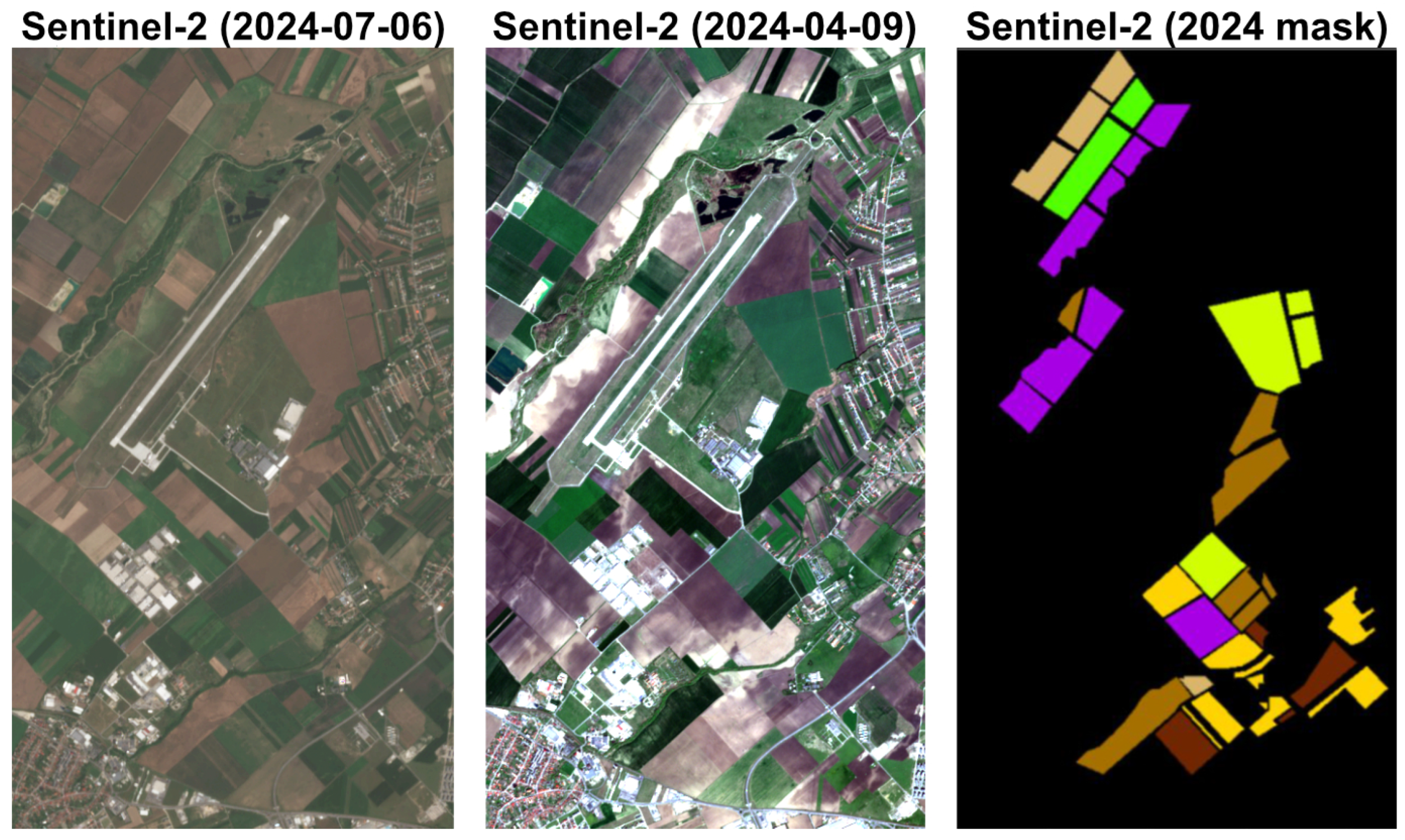
In Figure 2, two RGB visualizations of multispectral images, acquired on different dates within the same year are shown, along with their corresponding masks; each color represents one of the five crop types.

2.2. Principles of Crop Rotation

Crop rotation is a foundational principle of sustainable agriculture, aimed at enhancing soil health, managing pests and diseases, and improving crop productivity.
The core principles of crop rotation have long been established and thoroughly studied [25,26,27,28]. The more diversified the rotation is, the more long-term benefits appear [29].
It is a known fact that some plants benefit more from rotation than others. Wheat, for example, is highly dependent on its preceding crop, requiring early field clearance and low pathogen pressure. The best precursors are annual legumes (e.g., pea, bean, vetch) [30], which are harvested early and contribute biologically fixed nitrogen. Wheat should not follow barley or be continuously cropped due to shared pathogens. Continuous wheat should be avoided or mitigated with proper tillage, residue management, and pest control [31].
Corn is a relatively flexible crop in terms of rotation requirements, yet it responds positively to well-structured crop sequences. While it can tolerate short-term monoculture better than crops like wheat or sugar beet, continuous corn cultivation often leads to reduced yields [32], increased pest pressure, and a decline in soil health. Common issues in continuous corn systems include higher incidences of root-feeding pests (e.g., Diabrotica virgifera virgifera, the western corn rootworm), increased disease risks such as Fusarium and Gibberella stalk rot, and nutrient imbalances due to high nitrogen demand [33].
Pea is widely recognized as a highly beneficial crop in rotational farming systems due to its ability to fix atmospheric nitrogen through symbiosis with rhizobial bacteria. The inclusion of peas in crop rotations has been shown [34] to improve overall soil fertility, enhance yield stability of subsequent crops, and promote more sustainable and cost-effective agricultural practices.
Potato, though partially self-tolerant, remains vulnerable to major biotic threats. Viral infections like Potato virus Y (PVY) impair plant defenses and increase susceptibility to pests such as the Colorado potato beetle [35]. Late blight (Phytophthora infestans) remains the most destructive disease, causing up to USD 10 billion in annual losses [36]. The Colorado potato beetle, resistant to many insecticides, requires integrated control strategies. Crop rotations with legumes (e.g., peas, beans) improve soil health and increase potato yields by 21–28% over monoculture [37]. Four-year rotations (e.g., potato–oat–faba bean–potato) also boost yields and reduce disease incidence [38]. Early potato followed by winter cereals supports better soil preparation and nutrient availability.
Sugar beet should not be grown on the same field more frequently than once every four to six years due to its high susceptibility to soil-borne diseases and pests, particularly the beet cyst nematode (Heterodera schachtii) and root rot pathogens such as Aphanomyces cochlioides. Continuous sugar beet cultivation increases nematode populations and disease pressure, resulting in lower yields and root quality. Long-term field trials and farm surveys across Europe have demonstrated that crop rotations with non-host crops such as cereals, corn, or legumes, significantly suppress nematode populations and support sustainable sugar beet production. A rotation interval of at least four years is widely recommended [39,40] to mitigate these biotic stressors.
Rapeseed thrives when rotated after non-host cereals like wheat or barley, which interrupt the life cycle of soilborne pathogens such as Sclerotinia sclerotiorum. A four-year interval between rapeseed crops is advised [41], and sclerotia can survive in soil for up to seven years, underscoring the importance of long rotations. National guidelines further warn against following rapeseed with legumes or sunflower, which share pathogens like Sclerotinia, Alternaria, and Plasmopara, advocating instead for cereals as safer pre-crops. These recommendations [42] help prevent disease buildup by disrupting pathogen persistence, ensuring healthier crops and better yields.
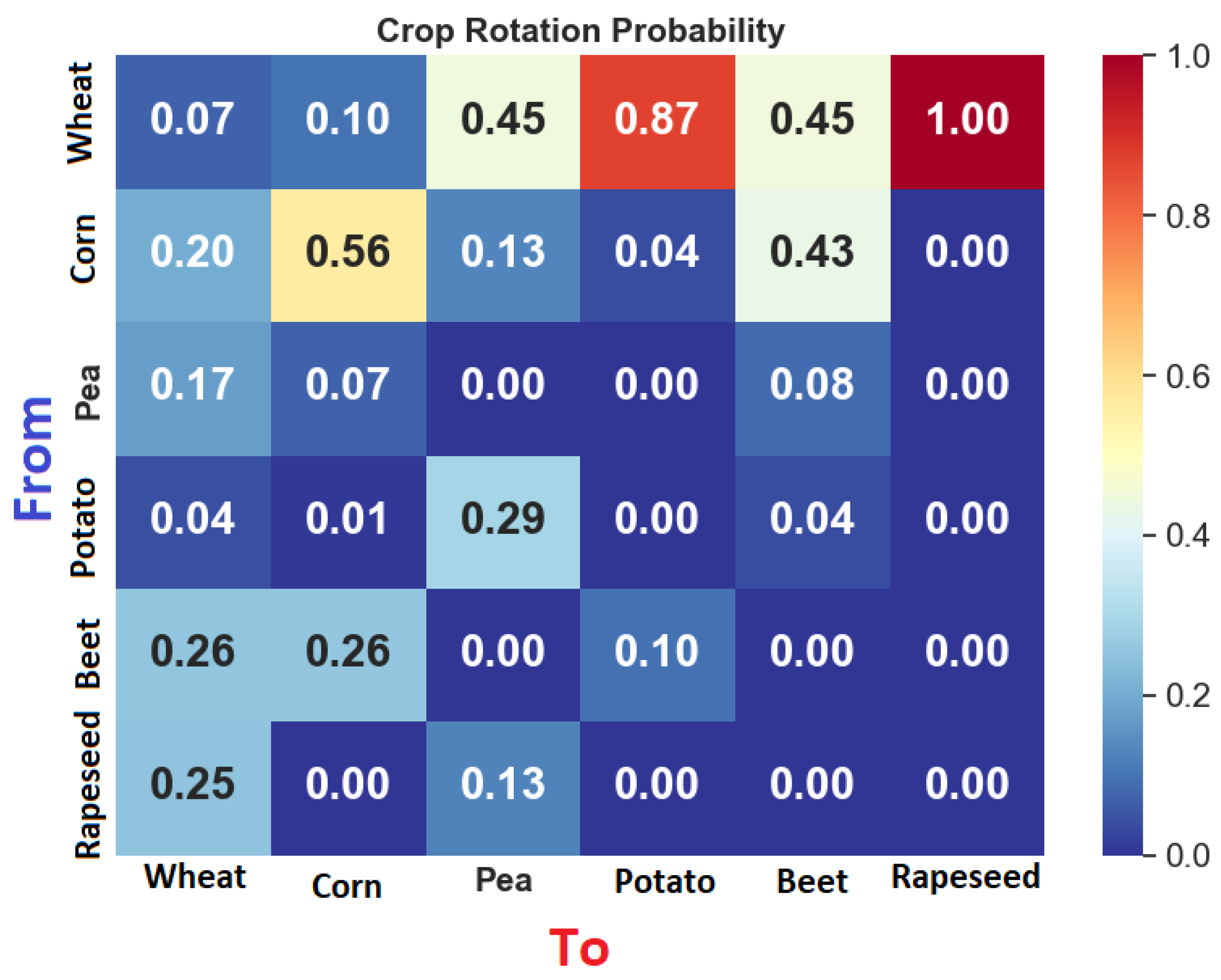
In Figure 3, the crop rotation derived from the labeled data of the DACIA5 dataset is illustrated. This real-life scenario demonstrates how different crops were rotated over a period of four years to simplify and better understand the main crop rotation patterns. Again, the rotation includes the following crops: wheat, corn, peas, potatoes, sugar beet, and rapeseed.

2.3. Romanian Crop Distribution

The DACIA5 dataset reflects a specific crop distribution, shaped by the conditions under which it was recorded. Limiting all experiments to this distribution poses challenges, as the Brașov area has unique climatic and geographical characteristics. Moreover, the recorded parcels belong to a Research and Development institute, which operates with different objectives than a typical commercial farm. For example, examining the rotation model in DACIA5 reveals instances where corn appears on the same parcel in consecutive years—an uncommon practice in general agriculture, but one that serves specific research purposes.
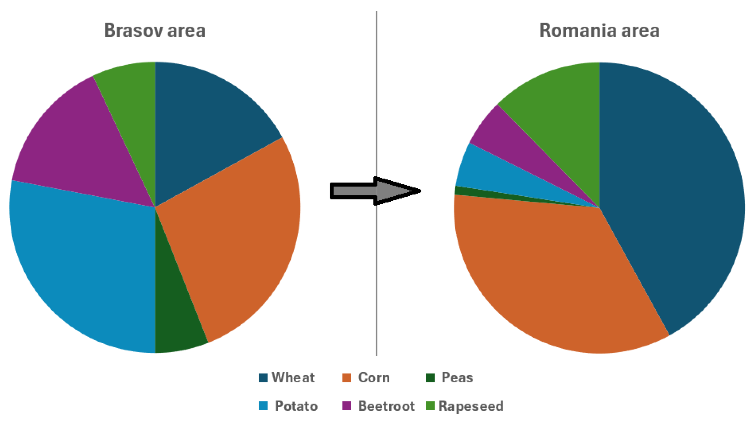
To modify the crop distribution, we refer to national Romanian agricultural statistics, which are published annually by the Ministry of Agriculture and available to the public [43]. For the crops considered in this study, their relative distribution—compared to that in the original DACIA5 dataset—is shown in Figure 4.

2.4. Sentinel-2 Pixel Simulation

The problem we are approaching here is two-fold. On the one hand, we have accurate data but for a particular farm/institute, and we need to extrapolate for another area. This is illustrated in Figure 4. The second is machine learning motivated: classifiers used to recognize crops need as much data as possible, and, in general, the best performance is achievable when classes (i.e., crops) are balanced in the training set.

2.4.1. 12D Pixel Synthesis

To synthesize new pixels for crops that are severely underrepresented, we used a variant of Gibbs Sampling [44]. Gibbs Sampling is a Markov Chain Monte Carlo algorithm used to generate samples from a multivariate probability distribution when direct sampling is difficult, but conditional distributions are known. Here, the purpose is to sample from a joint distribution p ( x 1 , x 2 , , x n ) , especially when it is hard to sample directly, but easy to sample from the conditionals p ( x i | x i 1 ) , where x i and x i 1 are dimensions of the probability. The key idea is that instead of updating all variables at once (as in Metropolis–Hastings), this Gibbs Sampling updates one variable at a time, keeping the previous fixed, using the conditional distributions.
In general, Gibbs Sampling assumes to draw x 1 i p x 1 | x 2 i 1 , x 3 i 1 , , x n i 1 ( x ) , which means that the current dimensions have a known dependence model with respect to previous considered dimensions. However, if the dependence structure is not well modeled, the space is high-dimensional with strongly dependent variables, Gibbs Sampling is often inefficient and potentially inaccurate [45,46]. An intuition about this phenomenon starts with the fact that when variables are highly correlated, Gibbs updates one dimension at a time. The sampler must traverse a narrow valley in the joint space, leading to extremely slow mixing—requiring many more iterations to converge, and it may become “stuck” in subregions of state space, never moving to other plausible areas. Additional methods that can model more complex dependencies—such as SMOTE (Synthetic Minority Oversampling Technique), Variational Autoencoders (VAE), and Generative Adversarial Networks (GAN)—do exist. However, these approaches typically require larger datasets and are significantly more complex to implement. For a comprehensive overview of such methods, we refer the reader to the survey by Figueira et al. [47].
To reach a compromise, we assume a dual band correlation: we start with some initial dimension, where the data is independent, and follow with the most correlated dimension, but always assuming that correlation is between pairs and not multiple. In this case, the used algorithm is described in Algorithm  1. The sample generation from a probability density function is performed with the Metropolis–Hastings algorithm, described in Algorithm 2.
Algorithm 1 Gibbs Sampling for pair of dimensions correlation.
  • Sample x 0 from p X 0 ( x ) , resulting x = [ x 1 , x 2 , , x n ] T
  •   For i = 0: N
  •   Generate sample x 1 i p x 1
  •   Generate sample x 2 i p x 2 | x 1 i
  •   …
  •   Generate sample x n i p x n | x n 1 i 1
  •    x = [ x 1 i , x 2 i , , x n i ] T
  • Return { x N b , x N b + 1 , , x N }
Algorithm 2 Metropolis–Hastings Algorithm
  • Given a current state x t :
  • Repeat for t = 1 , 2 , , T
  •   Propose a new state x q ( x | x t )
  •   Compute acceptance ratio:
  •      α ( x t , x ) = min ( 1 , π ( x ) · q ( x t · x ) π ( x t ) · q ( x | x t ) )
  •   Accept or reject:
  •     Generate u Uniform ( 0 , 1 )
  •     If  u < α , accept: x t + 1 = x
  •     else reject: x t + 1 = x

2.4.2. Practical Details

The simulation process began with real Sentinel-2 data, which provided up to 40 multispectral images per year—each capturing the same area across different months and days. Since the goal was to support a crop classification task, the data points had to be extracted with consideration for the specific crop’s sprouting and harvesting periods. For that matter, only the pixels showing signs of active green vegetation were selected.
Subsequently, the pixels needed to be separated by class, i.e., by the label-culture that was provided by the dataset makers. Each class contains pixels that are 12-dimensional. It is a known fact that Sentinel-2’s spectral band values are correlated with each other [48,49]. The sampler logic builds on this observation by leveraging the statistical dependencies between spectral bands.
The original dataset was analyzed, and two key pieces of information were extracted:
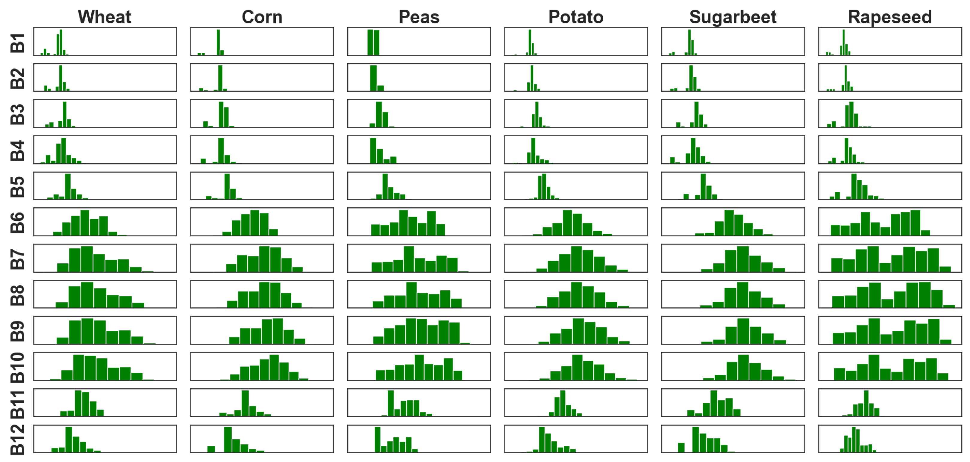
  • The histograms representing the pixel values distribution for each band within each agricultural crop, illustrated in Figure 5;
  • The co-occurrence matrices representing the joint histograms between selected adjacent bands.
Let us consider two Sentinel-2 spectral bands: band a (the initially selected band) and band b (its neighboring band). First, a value is chosen for band a. Then, based on this value, we estimate the value of band b using a conditional probability distribution, noted as q ( x b x a ) . This distribution reflects how values of band b typically occur when a certain value of band a is already known. In other words, the information from band a helps us make a more informed and likely choice for band b, based on how often certain combinations of values appear together in real data.
This process can then be repeated for each crop, allowing the value of one spectral band to be inferred based on another. Naturally, the first band in the sequence cannot depend on any previous one. Therefore, its value is generated using the overall distribution of that band for the specific crop class, as observed in the dataset.
The chosen band from which the generation process starts—assumed independent—was the green band (B3). This decision was based on several considerations. First, B3 is one of the bands with high signal-to-noise ratio and stable reflectance values across vegetation types, making it a reliable starting point for class-conditional generation [50]. Second, the green band (B3) effectively captures key physiological traits of crops, such as chlorophyll content and canopy structure [51].

2.5. Crop Rotation Simulation

Let us begin with two key observations. First, the DACIA5 dataset covers a finite number of years. To utilize data from the first year, we need to synthesize the previous crop label. Second, when synthesizing pixels, they are assigned a current label, but they also require a previous label to be compatible with our framework. Both observations highlight the need for an algorithmic method to generate meaningful previous labels. Additionally, since we aim to study specific crop rotation models and their impact on recognition, we must modify the previous crop labels accordingly—following a well-defined algorithmic approach.
In this case, the rotation is modeled as a Markov process (the rotation matrix from Figure 3 are Markov matrices), and we used the Metropolis–Hastings algorithm [52]. The latter is a Markov Chain Monte Carlo (MCMC) method used to sample from complex probability distributions when direct sampling is difficult. Its goal is that, given a target distribution π ( x ) (often known only up to a constant), the algorithm generates samples that approximate π ( x ) . The algorithm requires a proposal distribution: q ( x | x ) , a distribution used to propose the next state based on the current one and acceptance probability, and α ( x , x ) , which determines whether to accept or reject the proposed move. The algorithm is presented in Algorithm 2.
Using Algorithm 2 over a specific form of a rotation matrix, it generates labels, which tend to abide the distribution showed by matrix values.

2.6. Crop Identification

For crop identification, two models have been used. The first is a Random Forest, while the second is a Gradient Boosting Machine based on XGBoost implementation.
The Random Forest [53]—RF—classifier with 100 estimators was employed due to its robustness and reduced sensitivity to class imbalance. Random Forests, as ensemble methods, combine multiple decision trees trained on different random subsets of the data, which helps mitigate overfitting and improves generalization. Importantly, they handle unbalanced datasets relatively well compared to many other classifiers because each tree can capture minority class characteristics without being overwhelmed by the majority class.
Gradient Boosting Machine is employed in the form of eXtreme Gradient Boosting (XGBoost) [54], an optimized implementation of the original Gradient Boosting framework [55]. XGBoost is a type of ensemble learning method that combines multiple weak learners—typically decision trees—into a strong predictive model. Each successive tree is trained to correct the residual errors of the previous ensemble (a process known as boosting). XGBoost is particularly efficient due to its built-in support for parallel computation, enabling fast training on large-scale datasets.
From a mathematical perspective, XGBoost is an iterative procedure that begins with an initial prediction (commonly zero), and incrementally adds trees to minimize the prediction error. This process can be formalized as:
y i ^ = k = 1 K f k ( x i )
where y i ^ is the final predicted value for the ith instance (i.e., x i ), K is the number of trees in the ensemble, and f k ( x i ) is the prediction of the kth tree for the ith data point.
The objective function in XGBoost comprises two components: a loss function, which evaluates how well the model fits the training data, and a regularization term, which penalizes model complexity to prevent overfitting. The general form of the objective function is as follows:
L ( θ ) = i n l ( y i , y i ^ ) + k = 1 K Ω ( f k )
where l ( y i , y i ^ ) is the loss function based on the difference between the true value y i and the predicted value y i ^ , while the regularization term Ω ( f k ) discourages too complex trees. In our case, we have used cross entropy for l ( · ) .
When deciding how to split the nodes in the tree, the information gain for every possible split is calculated. In the canonical form, the information gain for a split is calculated as:
G a i n = 1 2 G L 2 H L + λ + G R 2 H R + λ ( G L + G R ) 2 H L + H R + λ γ
where G L and G R are the sums of gradients in the left and right child nodes, respectively, while H L and H R are the sums of Hessians in the left and right child nodes, respectively.
To incorporate the prior knowledge on crop rotation in the XGBoost model, we have made the following changes:
  • The loss residual error, l ( · ) , is not from y t , y i ( x i ^ ) directly, but from y i ( x i , y t 1 ) ^ . y t 1 is the previous crop in the same location:
    l ( y i , y i ^ ) = C E ( y i , y i ^ ) + C E ( 1 R [ y t 1 , i ] , y i ^ )
    where R [ i , y t 1 ] is the vector of rotation probabilities corresponding to the crop grown in the previous year at pixel i
  • the gradient and the Hessian are penalized if a tree sets the same prediction as the previous (i.e., y t 1 = = y i ^ ): G = G · α and, respectively, H = H · α , where G and H are the gradient total magnitude and respective hessian magnitude for an entire tree. The α constant is chosen to control the penalty. While values between 1.4 to 3.0 showed beneficial effect, the preferred value is 2.0 .
It should be noted that both used classifiers, RF and XGBoost, are able to predict the output as class probabilities.
The crop identification may be alternatively enhanced by incorporating crop rotation information. A simple way is to add it as a feature in the training set; however, in the evaluation, this approach has been found less effective.

Post-Prediction Processing with Crop Rotation Information

To further improve classification accuracy, crop rotation information was incorporated during the testing phase. While the rotation pattern for the DACIA5 dataset is known (see Figure 3), it is limited in scope, and our goal was to generalize the study beyond this specific case. Hence, a procedure was developed.
Specifically, after the classifier produces a probability distribution over all crop classes for each pixel, this distribution is adjusted based on the crop rotation probabilities derived from agronomic knowledge. The rotation matrix R, built from historical crop rotation data, encodes the likelihood of transitioning from one crop to another from one year to the next. For each pixel, the adjusted predicted label y rotation for pixel i is obtained as follows:
y rotation , i = arg max probs i × R [ y previous , i ]
Here, probs i is the vector of predicted probabilities for pixel i from the chosen classifier, R [ i , y previous ] is the vector of rotation probabilities corresponding to the crop grown in the previous year at pixel i, and the multiplication is performed element-wise. The label with the highest product value after this adjustment is selected as the new prediction.
The rotation matrix R was obtained using the following formula:
R i j = r max + 1 C i j α k = 1 n r max + 1 C i k α
where C i j , whose values are represented in Table 1, is a matrix that gives a score to each crop pair depending on the likelihood that that rotation will occur, r max = 5 is the maximum score within the C matrix, and the parameter α adjusts how strongly these tendencies influence the probabilities.
In Table 1, scores range from 1 (very favorable) to 5 (very difficult), reflecting the relative ease or advisability of rotating from one crop to another. For instance, rotations involving legumes such as peas followed by cereals like wheat or corn are highly favored (score = 1) due to their nitrogen-fixing capacity [30,56,57]. Conversely, rotations between cereals themselves, such as wheat and corn, receive lower ratings (score = 4), owing to limited benefits in terms of soil nutrient dynamics and the potential build-up of shared pests and diseases [58,59].
Alternative rotation matrices may be determined by selecting random values based on probabilities proportional to rotation scores.

3. Results

In the methods section we have introduced, mainly, two core contributions, which can be further extended. The core contributions are Sentinel Pixel Simulation and Crop identification based on crop rotation models. Before developing the experimental results, we provide details of implementation.

3.1. Implementation

All computations were performed using Python version 3.10.12, with libraries such as NumPy (v1.21.5) and SciPy (v1.9.1) for numerical calculations and Monte Carlo simulations. The XGBoost classifier was implemented using the XGBoost library (v3.0.2), while the Random Forest classifier was based on scikit-learn (v0.19.2).
The DACIA5 dataset includes approximately 3.5 million real pixels, along with 2.5 synthesized pixels. Various scenarios were tested, but on average, a full training/testing cycle took about 1 h for the Random Forest model. XGBoost, which benefits from a more optimized implementation, required approximately 100 s after data loading. For XGBoost, we ensured that the modified loss function relied on vectorized operations to avoid moving data between the built-in C backend and Python; otherwise, it may take up to 9 h.
No GPU acceleration was used, and all experiments were conducted using single-threaded processing.

3.2. Sentinel-2 Pixel Simulation

Sentinel-2 Pixel Simulation with crop dependence is evaluated in two scenarios. First, in this subsection, we compare how similar the simulated pixels are to the original ones. In the next subsection, we examine their impact on crop identification.
The similarity of simulated pixels with original pixels is based on the Mahalanobis distance. The Mahalanobis distance is a measure of the distance between a point x and a distribution Q ; oftentimes, the distribution Q is assumed to be multivariate Gaussian of μ mean and Σ covariance matrix. It is calculated as follows:
M D ( x , Q μ , Σ ) = ( x μ ) T Σ 1 1 ( x μ )
The MD is a multivariate generalization of the square of the standard score computed as:
z = x μ σ
The standard score shows how many standard deviations away x is from the mean of Q . This property makes it suitable to compare compactness and sparsity among clusters originating in differently dimensional spaces such as the 12-dimensional multispectral Sentinel pixel space.
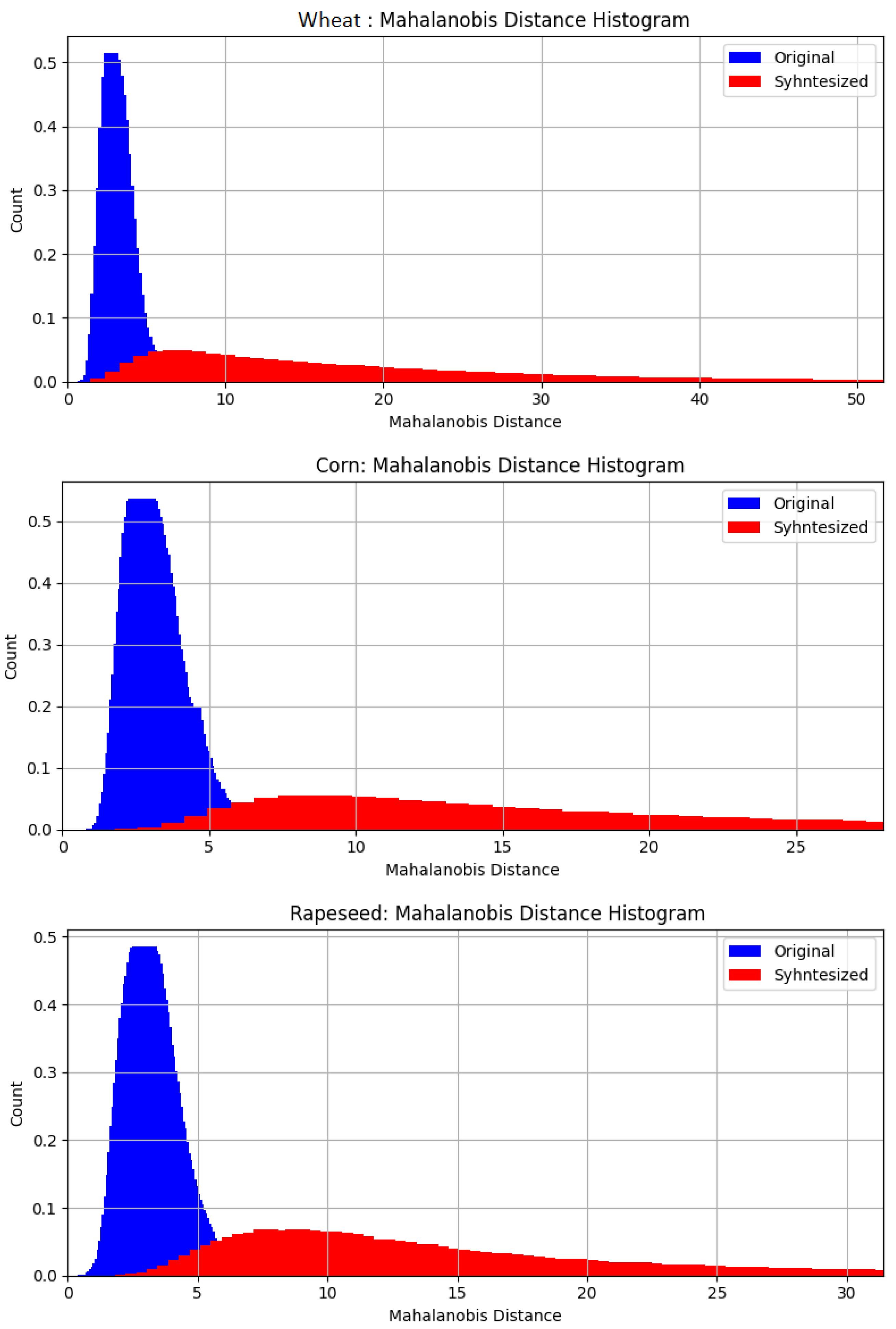
In this subsection, we model the original pixel density function as a Gaussian and compute (i) the distance from every original pixel to the original pixel density and (ii) the distance from every simulated pixel to the original pixel density. The histogram of distances may be followed for the three main crops in Figure 6.
Before analyzing the results, it is important to emphasize that during the simulation process, the dimensions corresponding to spectral bands are generated sequentially, each assuming correlation only with the previously considered band. No multiband correlation or joint dependence is modeled, due to the limitations of the Gibbs Sampling approach (as explained in Section 2). In contrast, the Mahalanobis distance is a multidimensional metric that compares a 12-dimensional pixel to a distribution defined in the same 12-dimensional space. In this computation, inter-band correlations are fully accounted for, based on the original data statistics, and no further modeling constraints are imposed.
Several observations can be made regarding the results. First, we note that for all crops shown, the behavior of the simulation is consistent. A small percentage of the simulated pixels overlap with the original distribution, while the majority are slightly farther away. Considering that original pixels are typically within a Mahalanobis distance of five from the center of the original distribution, the synthesized pixels span a larger range: up to 10 times that distance for wheat (and similarly for peas, potatoes, and sugar beet), 5 times for corn, and 6 times for rapeseed.
A second observation is that the relevance of synthesized pixels depends on the intended application. For example, when preparing a dataset to train a classifier, it is beneficial to include pixels that are somewhat farther from the original distribution to fill gaps between crop clusters. We stress that synthesized data is expected to differ from real data, but within reasonable bounds. There are two key limitations to consider:
  • If the synthesized data is too similar to the original, it adds little value during the machine learning process, as it merely replicates existing patterns without expanding the feature space.
  • If it is too different, it may introduce unrealistic crop representations, potentially confusing the classifier and degrading performance.
Therefore, a balance must be struck between generating data that is “too similar” and data that is “too different”.
In our experiments, we considered pixels up to three times the original distance. However, if a larger number of crops are included, a lower threshold might be more appropriate, as the feature space could already be well covered. Conversely, if the goal is to obtain pixels highly similar to the original—such as for generating clean clusters or histograms—only pixels within the original range should be selected.

3.3. Crop Identification

For crop identification, evaluation is performed under two scenarios. The first scenario involves testing exclusively on real data from the DACIA5 dataset. Within this scenario, two cases are considered: (1) testing on the 2022 data, which includes actual previous crop information, and (2) testing on the first available year (2020), where the previous crop is synthesized using a model that more closely reflects a commercial farming setup. Crop identification only inside DACIA5 scenario is referred to as the “DACIA5 Test”.
The second scenario involves testing on a dataset with a different crop distribution. Here, the distribution of the test set is modified using synthesized pixels to match national-level crop proportions. This scenario is referred to as the Romania Test.

3.3.1. DACIA5 Test

In this scenario, the baseline version consists of using all data from a selected test year, while data from the remaining years are included in the training set. When testing is performed on the 2022 data, the previous crop labels are real; however, for 2020, the previous labels are synthesized using various rotation matrices.
When synthesized pixels are added to the training set, the goal is to balance class distributions. Given that corn and rapeseed are naturally more frequent, the proportion of the other three crops was increased to approximately 10%.
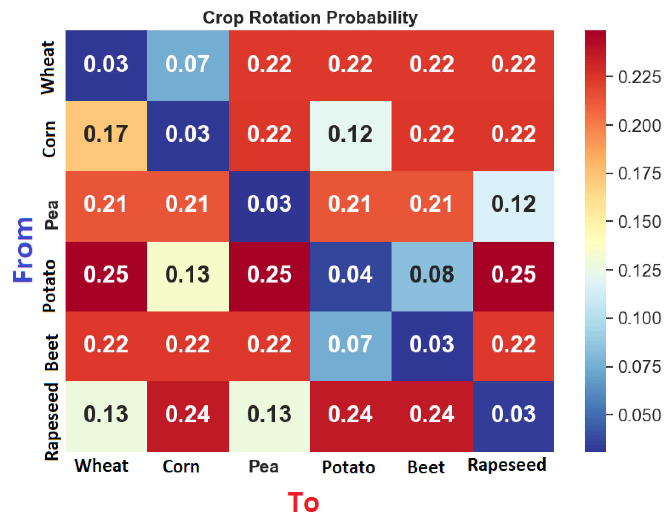
The comparative performance when testing on 2022 data is shown in Table 2. As a general trend, the classifiers perform similarly, with XGBoost having a slight advantage, particularly due to its faster execution. A well-designed rotation model ( R 1  Figure 7)—where the current crop differs from the previous one—improves recognition accuracy. In contrast, scenarios where the current crop is the same as the previous (as seen in the DACIA5 dataset due to research-driven practices— R 0  Figure 3) offer less benefit. Adding synthesized data also contributes to improved performance, though the impact in this case is relatively modest.
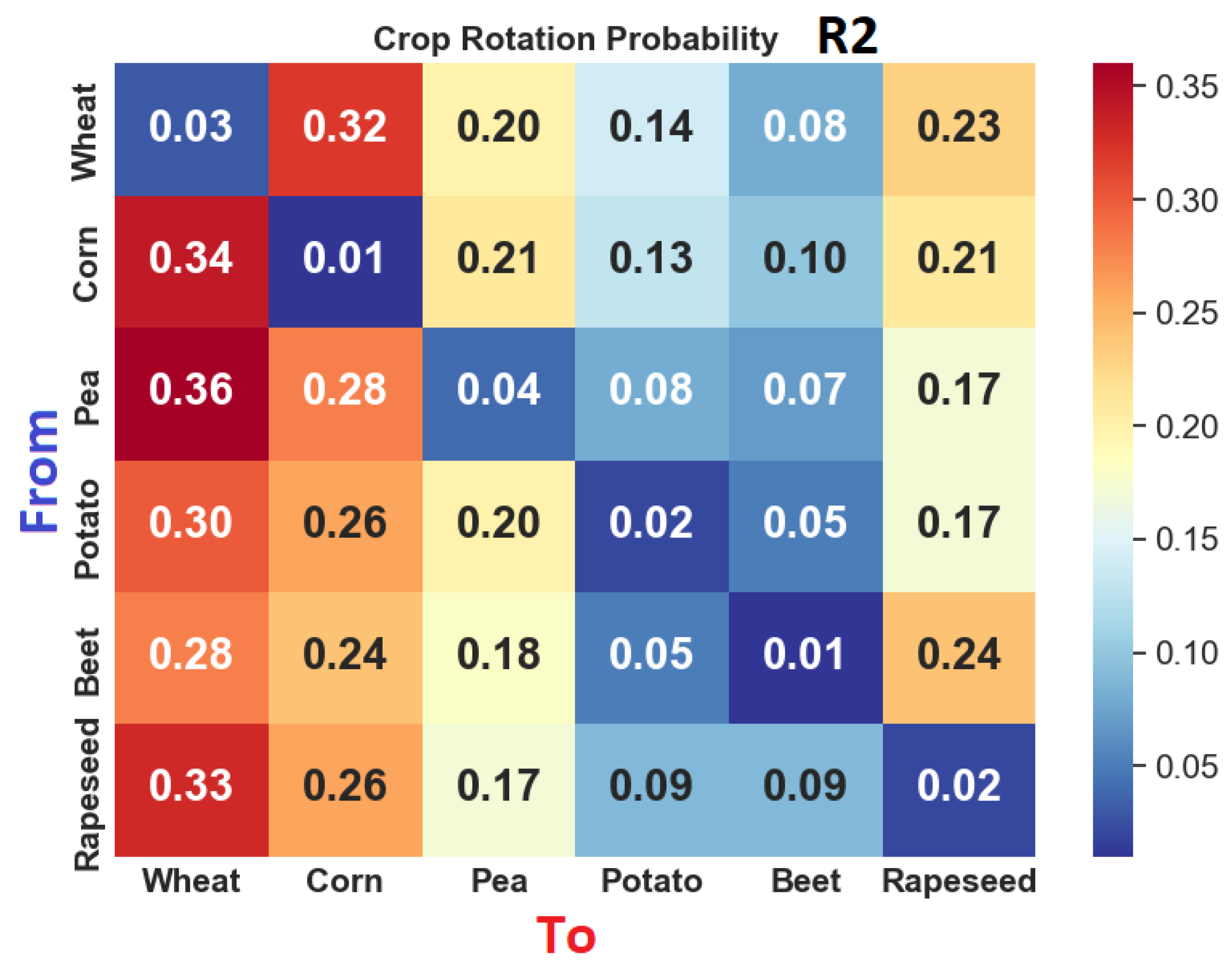
The comparative performance when testing on 2020 data with synthetic previous crop is shown in Table 3. The rotation models used to synthesize previous labels are R 1 (Figure 7) and R 2 (Figure 8).
After these result analyses, the general trend continues: comparable classifier performance; more diverse rotation; better improvement; not all rotation information can be added. Again, by adding synthesized data, performance improves, although the impact in this case is more pronounced.
Table 4. Evaluation on 2020 data combined with synthetic to match the relative distribution specific to Romania.
ClassifierRotation ModelSyntheticAccuracy [%]
XGBNoNo65.64
XGBPost-R1No66.14
XGB-lossdefaultNo68.15
XGB-lossdef + post-R1No67.95
XGB-lossdef + post-R1Yes70.15
XGB-lossdef + post-R2No69.22
XGB-lossdef + post-R2Yes71.14
RFNoNo64.22
RFPost-R1No65.96
RFPost-R1Yes68.04
To emphasize the effect of rotation, we also considered more detailed evaluation, where each of the years is taken into test one at a time. Rotation data is the one from Figure 7. No synthetic data is used, and the results presented in Table 5 highlight the consistent benefit of integrating crop rotation knowledge into the classification process. Specifically, when comparing the “Real pixels (no rotation)” scenario to the “Real pixels (with rotation)” scenario across all years, it is evident that the inclusion of rotation-adjusted probabilities generally leads to improved classification performance.
For four out of the five years (2020, 2021, 2022, and 2024), the accuracy increases when rotation constraints are applied. For example, in 2020, the accuracy rises from 58.33% to 61.94%, and in 2022—from 55.12% to a notably higher 63.26%. These gains reflect the ability of the rotation probability matrix to correct or regularize the classifier’s outputs by leveraging agronomic transition likelihoods. This post-processing step helps reduce confusion between crops that are unlikely to follow each other, effectively embedding prior domain knowledge into the decision pipeline.
The only exception is 2023, where a slight decrease in accuracy is observed after applying rotation (63.89% without vs. 62.56% with rotation). This deviation, although marginal, may suggest that the model’s raw predictions in that particular year were already strongly aligned with the true crop transitions or that rotation patterns in 2023 diverged from historical norms captured in the matrix.
The results of the rotation are shown in Figure 9, which presents a visual comparison across three classification outputs over distinct spatial crop regions. The figure is organized into three columns: the first displays the ground truth labels for each selected region, serving as the reference standard, the second column shows the predictions made by the classifier without the use of crop rotation constraints, while the third column integrates domain knowledge through a crop rotation probability matrix, adjusting predictions based on the previous year’s crop.
From the comparison, it is evident that incorporating crop rotation information improves classification in several cases. Notably, some pixels initially misclassified as corn are correctly re-identified as sugar beet, and rapeseed is more accurately retrieved from former wheat fields, reflecting agronomic plausibility in crop succession. However, despite these improvements, the post-rotation predictions are not universally accurate. Certain areas still exhibit confusion, particularly in regions where spectral signatures overlap or where rotation probabilities are less definitive.
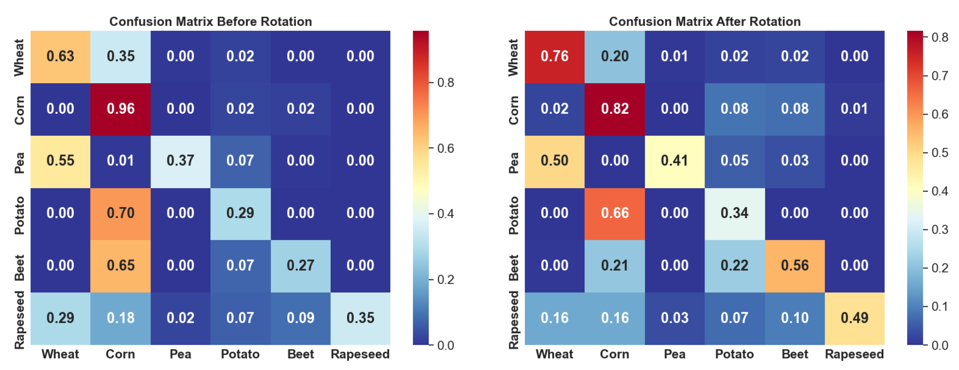
In addition to the visual assessment, the quantitative evaluation presented in the confusion matrix (Figure 10 right) corroborates the observed improvements seen in Figure 9. The comparison between the matrices before and after rotation (Figure 10 left) highlights that the crop rotation notably reduces misclassifications between agronomically linked crop pairs. Specifically, the confusion between sugar beet and corn diminishes, and similarly, the classification of rapeseed versus wheat improves, aligning with common crop succession practices.

3.3.2. Romania Test

In this scenario, the testing set consists of all pixels from the DACIA5 dataset for the year 2020, extended to match the nominal crop distribution using synthesized pixels. All pixels from the other years are included in the training set, and, when specified, synthesized pixels are also added to balance the distribution, as previously described. For the training set, all previous crop labels are generated using a rotation model (which may be either R1 or R2). The results are shown in Table 4.
With regard to the results obtained on the dataset expanded using synthesized data to reflect the national Romanian crop distribution, several important observations can be made. First, it is worth noting that synthesized data has been included in both the training and testing sets. As highlighted by the Mahalanobis distance analysis, these synthetic pixels may differ slightly from the real ones in spectral characteristics. However, we consider this a realistic and meaningful condition, as datasets collected from different geographic regions often exhibit specific, localized features. From a machine learning standpoint, this variation can be advantageous, since the classifier is exposed during training to examples that are similar in nature to those it will encounter during testing.
This setup mimics real-world applications, where models trained on one region or dataset are expected to generalize to others. The slight discrepancies between synthetic and real data serve to improve the robustness of the learning process rather than detract from it.
In addition to these considerations, we emphasize the overall consistency observed in the experimental results. When both classifiers—Random Forest and XGBoost—were applied under the same conditions, their performance levels were generally aligned, with XGBoost showing a slight edge, particularly in terms of speed. The inclusion of crop rotation information contributed significantly to improved recognition accuracy. This improvement was more pronounced in scenarios where crop rotation patterns were diverse and the likelihood of a crop repeating from the previous year was lower. In contrast, less diverse or repetitive rotation patterns offered fewer benefits.
Moreover, when additional synthetic data was introduced—entirely independent between the training and testing sets—the positive effect on identification performance became even more noticeable. This reinforces the idea that both data augmentation and the intelligent use of prior agronomic knowledge (in this case, crop rotation models) can be effective strategies to boost classification performance in agricultural remote sensing tasks.

4. Discussion and Limitations

The methodology, solutions, and conclusions presented in this study have certain limitations, which we aim to analyze in this section. However, let us first review some findings.
One key insight is that incorporating previous crop labels improves classification performance, particularly when implemented through a custom loss function that penalizes deviations from historically plausible transitions. This aligns with prior work showing that temporal context enhances crop identification [60,61]. Our results extend this line of research by simulating realistic crop sequences and evaluating their effect on classification performance without the need for long, labeled time series. Since crop rotations are well established, models such as Random Forests that account for heterogeneity in crop classification have been previously used [9]. A common approach relies on Markov chains [11]. We adopt a similar conditional Markov chain model, but introduce a different method for incorporating previous crop data. Nonetheless, our findings are consistent with previous studies [9,11,18,60,61], which highlight that modeling heterogeneity in crop prediction contributes to improved accuracy.

4.1. Rotation Model

Crop rotation is a well-established agricultural practice aimed at improving soil quality and mitigating environmental degradation. Although it has been used for a long time, it is still not fully understood or optimized. Many research groups continue to study specific aspects of rotation—such as its effects on nutrients, water usage, and yield [29,33,38,58,62]. Their findings may further refine or even challenge current rotation models.
Moreover, what is optimal from an environmental perspective is not always optimal from an economic one. In some regions, certain crops are more economically viable than others. Climate change and shifting market demands can also lead to changes in which crops are cultivated, requiring rotation patterns to adapt. For instance, the Bârsa premontane plain—which has been known locally as the “Potato Country”—sees increasing temperatures which translate to a higher percentage of land being cultivated with wheat, corn, and rapeseed, while the percentages of land with potato and sugar beet decrease. Agricultural engineers and farmers must balance ethical principles with practical considerations, meaning the actual application of crop rotation may vary over time. These factors can influence the applicability of our proposed methodology.
A main limitation of the model assumed is that the simulated data assumes ideal rotation logic, while in real-world scenarios, crop changes depend on many uncertain factors (economic, environmental, etc.). Moreover, while synthetic labeling helps explore model behavior, it does not fully replace the complexity and variability of real annotated datasets [63]. A future direction would be to integrate rotation probabilities derived from historical geospatial records, such as national registries.

4.2. Data Specificity

Our study uses data collected from a specific geographic location, which introduces some inherent limitations. While we have made efforts to ensure generalization, certain data characteristics—some of which are not yet fully understood—may limit broader applicability. For example, wheat varieties are adapted to particular climates and terrains [64,65]. Wheat grown in lowland, humid areas differs from wheat grown at higher elevations, which can affect both identification and data synthesis [64].
To address this, we introduced the Mahalanobis distance as a control mechanism to guide how similar the synthesized data should be to the original. If geographic or climatic conditions change and it is known that the data should diverge, this can be reflected by adjusting the Mahalanobis distance parameter accordingly.

4.3. Synthesis by Monte Carlo

In the pixel synthesis process, we employed a Gibbs Sampler under the assumption of only pairwise conditional dependence. This is a limiting factor, as a full joint model capturing dependencies across all 12 dimensions would likely yield more accurate results.
However, when the dependence structure is complex or poorly specified—and the space is high-dimensional with strongly correlated variables—Gibbs Sampling tends to be inefficient and potentially inaccurate [45,46]. The underlying issue stems from the fact that Gibbs Sampling updates one dimension at a time. In cases of high correlation, this results in the sampler navigating a narrow ridge in the joint probability space, leading to extremely slow mixing. Consequently, the sampler may require a large number of iterations to converge and can become “stuck” in subregions of the state space, failing to explore other plausible configurations.
Alternative methods capable of modeling more complex dependencies—such as SMOTE (Synthetic Minority Oversampling Technique), Variational Autoencoders (VAE), and Generative Adversarial Networks (GANs)—are available [47]. However, these techniques generally demand larger datasets and are considerably more complex to implement.

4.4. Machine Learning Perspective

From a machine learning standpoint, our study focused on two classifiers that produced similar results, supporting the general validity of our conclusions. However, many other learning algorithms exist, and applying them may lead to slightly different outcomes; previous works in the same direction included Random Forest [9], neural networks [18], and other classifiers. This presents an opportunity for future exploration and validation using alternative models.
Crop relative frequency often varies by region. Some areas are well known for grain production, while others specialize in fruits or vegetables. From a machine learning perspective, distinguishing between crop types typically benefits from a more balanced dataset. However, the need for class balance depends on the specific learning algorithm used. Algorithms like Gradient Boosting Machines and Random Forests are generally more tolerant of class imbalance, while others—such as Support Vector Machines—are more sensitive to it. Therefore, when using data synthesis to improve crop identification, the approach should be tailored to the specific classifier employed.
Another point is model generalizability. Although the custom XGB loss improves performance on known crops and regions, its parameters (e.g., penalty weighting) may require tuning for different landscapes or cropping systems. This introduces a trade-off between model complexity and interpretability, as also noted in other learning approaches for agriculture [66,67].
Finally, while the proposed method does not introduce a new classification algorithm, it demonstrates how prior agricultural knowledge can be embedded into modern classification frameworks in a principled way. This highlights an opportunity to bridge remote sensing with agronomic modeling—an intersection still under-explored in many operational systems.

5. Conclusions

In this paper, we analyzed the impact of a crop rotation model on the crop identification problem. We began with an accurately annotated dataset, DACIA5, and, recognizing its limitations, introduced a synthesis mechanism capable of generating realistic pixels for known crops. This allows the crop distribution to be reshaped to match any desired scenario.
To study the implications of incorporating a rotation model into identification, we proposed a method for synthesizing previous crop labels for any simulated pixel. The crop rotation model is then integrated with the classifier. Specifically, for the Gradient Boosting Machine, we embedded the concept of crop change into the loss function by penalizing predictions that repeat the previous year’s crop.
All proposed solutions were tested on both real and simulated data with positive results. We found that the simulated pixels closely resemble real ones, and the Mahalanobis distance can serve as both a similarity measure and a control mechanism during data generation for targeted purposes. Regarding the rotation model, it encodes the prior assumption that the same crop is not typically cultivated on the same parcel in consecutive years. When properly incorporated, this information improves the overall recognition rate. The use of simulated pixels further enhances performance—by up to a notable 10%.

Author Contributions

Conceptualization, C.F., M.I. and A.N.; methodology, C.F., M.I. and A.N.; software, A.N. and A.R.; validation, C.F. and M.I.; formal analysis, C.F.; investigation, A.N., A.R., C.F. and M.I.; resources, M.I.; data curation, A.N. and A.R.; writing—original draft preparation, A.N.; writing—review and editing, C.F. and M.I.; visualization, A.N. and C.F.; supervision, M.I.; project administration, M.I.; funding acquisition, M.I. All authors have read and agreed to the published version of the manuscript.

Funding

The research was funded by the European Union. The AI4AGRI project received funding from the European Union’s Horizon Europe research and innovation programme under the grant agreement no. 101079136.

Data Availability Statement

The datasets generated and/or analyzed during the current study are available from the corresponding authors on reasonable request. The DACIA5 dataset is publicly available at https://zenodo.org/records/14915950 (accessed on 15 June 2025).

Acknowledgments

The authors would like to express their sincere gratitude to Octavian Racoviteanu for their patience in explaining meaningful insights in agriculture planning.

Conflicts of Interest

The authors declare no conflicts of interest.

Abbreviations

The following abbreviations are used in this manuscript:
AIArtificial Intelligence
CECross-Entropy
GBMGradient Boosting Machine
INCDCSZNational Institute of Research and Development for Potato and Sugar Beet
LPISLand Parcel Identification Systems
MCMonte Carlo
MCMCMarkov Chain Monte Carlo
MDMahalanobis distance
NIRNear Infrared
RFRandom Forest
RSRemote Sensing
SARSynthetic Aperture Radar
XGBoosteXtreme Gradient Boosting

References

  1. Aijaz, N.; Lan, H.; Raza, T.; Yaqub, M.; Iqbal, R.; Pathan, M.S. Artificial intelligence in agriculture: Advancing crop productivity and sustainability. J. Agric. Food Res. 2025, 20, 101762. [Google Scholar] [CrossRef]
  2. Victor, B.; Nibali, A.; He, Z. A systematic review of the use of Deep Learning in Satellite Imagery for Agriculture. IEEE J. Sel. Top. Appl. Earth Obs. Remote Sens. 2024, 18, 2297–2316. [Google Scholar] [CrossRef]
  3. Wu, B.; Meng, J.; Li, Q.; Yan, N.; Du, X.; Zhang, M. Remote sensing-based global crop monitoring: Experiences with China’s CropWatch system. Int. J. Digit. Earth 2014, 7, 113–137. [Google Scholar] [CrossRef]
  4. Boryan, C.; Yang, Z.; Mueller, R.; Craig, M. Monitoring US agriculture: The US department of agriculture, national agricultural statistics service, cropland data layer program. Geocarto Int. 2011, 26, 341–358. [Google Scholar] [CrossRef]
  5. Schneider, M.; Schelte, T.; Schmitz, F.; Körner, M. EuroCrops: The Largest Harmonized Open Crop Dataset Across the European Union. Sci. Data 2023, 10, 612. [Google Scholar] [CrossRef]
  6. Blickensdörfer, L.; Schwieder, M.; Pflugmacher, D.; Nendel, C.; Erasmi, S.; Hostert, P. Mapping of crop types and crop sequences with combined time series of Sentinel-1, Sentinel-2 and Landsat 8 data for Germany. Remote Sens. Environ. 2022, 269, 112831. [Google Scholar] [CrossRef]
  7. Qiu, B.; Lin, D.; Chen, C.; Yang, P.; Tang, Z.; Jin, Z.; Ye, Z.; Zhu, X.; Duan, M.; Huang, H.; et al. From cropland to cropped field: A robust algorithm for national-scale mapping by fusing time series of Sentinel-1 and Sentinel-2. Int. J. Appl. Earth Obs. Geoinf. 2022, 113, 103006. [Google Scholar] [CrossRef]
  8. Băicoianu, A.; Plajer, I.; Debu, M.; Ștefan, F.M.; Ivanovici, M.; Florea, C.; Cațaron, A.; Coliban, R.M.; Popa, S.; Oprisescu, S.; et al. DACIA5: A Sentinel-1 and Sentinel-2 dataset for agricultural crop identification applications. Big Earth Data 2025, 1–32. [Google Scholar] [CrossRef]
  9. Wang, X.; Tang, Q.; Yang, K. Improving crop rotation classification using a random forest model incorporating spatial heterogeneity. Geocarto Int. 2024, 39, 2384473. [Google Scholar] [CrossRef]
  10. Yang, L.; Song, M.; Zhu, A.X.; Qin, C.; Zhou, C.; Qi, F.; Li, X.; Chen, Z.; Gao, B. Predicting soil organic carbon content in croplands using crop rotation and Fourier transform decomposed variables. Geoderma 2019, 340, 289–302. [Google Scholar] [CrossRef]
  11. Giordano, S.; Bailly, S.; Landrieu, L.; Chehata, N. Improved crop classification with rotation knowledge using Sentinel-1 and-2 time series. Photogramm. Eng. Remote Sens. 2020, 86, 431–441. [Google Scholar] [CrossRef]
  12. Quinton, F.; Landrieu, L. Crop rotation modeling for deep learning-based parcel classification from satellite time series. Remote Sens. 2021, 13, 4599. [Google Scholar] [CrossRef]
  13. Upcott, E.V.; Henrys, P.A.; Redhead, J.W.; Jarvis, S.G.; Pywell, R.F. A new approach to characterising and predicting crop rotations using national-scale annual crop maps. Sci. Total Environ. 2023, 860, 160471. [Google Scholar] [CrossRef]
  14. Liu, Y.; Yu, Q.; Zhou, Q.; Wang, C.; Bellingrath-Kimura, S.D.; Wu, W. Mapping the complex crop rotation systems in Southern China considering cropping intensity, crop diversity, and their seasonal dynamics. IEEE J. Sel. Top. Appl. Earth Obs. Remote Sens. 2022, 15, 9584–9598. [Google Scholar] [CrossRef]
  15. Wang, P.; Xie, W.; Ding, L.; Zhuo, Y.; Gao, Y.; Li, J.; Zhao, L. Effects of maize–crop rotation on soil physicochemical properties, enzyme activities, microbial biomass and microbial community structure in Southwest China. Microorganisms 2023, 11, 2621. [Google Scholar] [CrossRef]
  16. Kussul, N.; Deininger, K.; Shumilo, L.; Lavreniuk, M.; Ali, D.A.; Nivievskyi, O. Biophysical impact of sunflower crop rotation on agricultural fields. Sustainability 2022, 14, 3965. [Google Scholar] [CrossRef]
  17. Xing, H.; Chen, B.; Lu, M. A sub-seasonal crop information identification framework for crop rotation mapping in smallholder farming areas with time series sentinel-2 imagery. Remote Sens. 2022, 14, 6280. [Google Scholar] [CrossRef]
  18. Barriere, V.; Claverie, M.; Schneider, M.; Lemoine, G.; d’Andrimont, R. Boosting crop classification by hierarchically fusing satellite, rotational, and contextual data. Remote Sens. Environ. 2024, 305, 114110. [Google Scholar] [CrossRef]
  19. Dong, Z.; Yao, L.; Bao, Y.; Zhang, J.; Yao, F.; Bai, L.; Zheng, P. Prediction of soil organic carbon content in complex vegetation areas based on CNN-LSTM model. Land 2024, 13, 915. [Google Scholar] [CrossRef]
  20. Chinembiri, T.S.; Mutanga, O.; Dube, T. A multi-source data approach to carbon stock prediction using Bayesian hierarchical geostatistical models in plantation forest ecosystems. GISci. Remote Sens. 2024, 61, 2303868. [Google Scholar] [CrossRef]
  21. Wu, Y.; Knudby, A.; Lapen, D. Topography-adjusted Monte Carlo simulation of the adjacency effect in remote sensing of coastal and inland waters. J. Quant. Spectrosc. Radiat. Transf. 2023, 303, 108589. [Google Scholar] [CrossRef]
  22. Radoux, J.; Chomé, G.; Jacques, D.C.; Waldner, F.; Bellemans, N.; Matton, N.; Lamarche, C.; d’Andrimont, R.; Defourny, P. Sentinel-2’s potential for sub-pixel landscape feature detection. Remote Sens. 2016, 8, 488. [Google Scholar] [CrossRef]
  23. Abdelmoula, H.; Kallel, A.; Roujean, J.L.; Gastellu-Etchegorry, J.P. Dynamic retrieval of olive tree properties using Bayesian model and Sentinel-2 images. IEEE J. Sel. Top. Appl. Earth Obs. Remote Sens. 2021, 14, 9267–9286. [Google Scholar] [CrossRef]
  24. Makhloufi, A.; Kallel, A. Inversion of a new designed ANN-based 3-D-RTM emulator by continuous MCMC technique to monitor crop biophysical properties using sentinel-2 images. IEEE Trans. Geosci. Remote Sens. 2023, 61, 1–14. [Google Scholar] [CrossRef]
  25. Weir, W.W. A Study of the Value of Crop Rotation in Relation to Soil Productivity; US Department of Agriculture: Washington, DC, USA, 1926; Volume 1377. [Google Scholar]
  26. Bullock, D.G. Crop rotation. Crit. Rev. Plant Sci. 1992, 11, 309–326. [Google Scholar] [CrossRef]
  27. Tanveer, A.; Ikram, R.M.; Ali, H.H. Crop rotation: Principles and practices. In Agronomic Crops: Volume 2: Management Practices; Springer: Singapore, 2019; pp. 1–12. [Google Scholar]
  28. Shah, K.K.; Modi, B.; Pandey, H.P.; Subedi, A.; Aryal, G.; Pandey, M.; Shrestha, J. Diversified crop rotation: An approach for sustainable agriculture production. Adv. Agric. 2021, 2021, 8924087. [Google Scholar] [CrossRef]
  29. Bowles, T.M.; Mooshammer, M.; Socolar, Y.; Calderón, F.; Cavigelli, M.A.; Culman, S.W.; Deen, W.; Drury, C.F.; y Garcia, A.G.; Gaudin, A.C.; et al. Long-term evidence shows that crop-rotation diversification increases agricultural resilience to adverse growing conditions in North America. One Earth 2020, 2, 284–293. [Google Scholar] [CrossRef]
  30. Mesfin, M.; Tekalign, A.; Fikre, A.; Yirga, C.; Jembere, T.; Getahun, T. Potentials of legumes rotation on yield and nitrogen uptake of subsequent wheat crop in northern Ethiopia. Heliyon 2023, 9, e16684. [Google Scholar] [CrossRef] [PubMed]
  31. Ridgman, W.J.; Walters, D.E. A comparison of growing wheat continuously with growing wheat in a four-course rotation. J. Agric. Sci. 1982, 99, 139–143. [Google Scholar] [CrossRef]
  32. Yuan, M.; Bi, Y.; Han, D.; Wang, L.; Wang, L.; Fan, C.; Zhang, D.; Wang, Z.; Liang, W.; Zhu, Z.; et al. Long-Term Corn–Soybean Rotation and Soil Fertilization: Impacts on Yield and Agronomic Traits. Agronomy 2022, 12, 2554. [Google Scholar] [CrossRef]
  33. Carrière, Y.; Brown, Z.; Aglasan, S.; Dutilleul, P.; Carroll, M.; Head, G.; Tabashnik, B.E.; Jørgensen, P.S.; Carroll, S.P. Crop rotation mitigates impacts of corn rootworm resistance to transgenic Bt corn. Proc. Natl. Acad. Sci. USA 2020, 117, 18385–18392. [Google Scholar] [CrossRef]
  34. Tejendra Chapagain, A.R. Barley—pea intercropping: Effects on land productivity, carbon and nitrogen transformations. Field Crops Res. 2014, 166, 18–25. [Google Scholar] [CrossRef]
  35. Petek, M.; Rotter, A.; Kogovsek, P.; Baebler, S.; Mithofer, A.; Gruden, K. Potato virus Y infection hinders potato defence response and renders plants more vulnerable to Colorado potato beetle attack. Mol. Ecol. 2014, 23, 5378–5391. [Google Scholar] [CrossRef]
  36. Dong, S.M.; Zhou, S.Q. Potato late blight caused by Phytophthora infestans: From molecular interactions to integrated management strategies. J. Integr. Agric. 2022, 21, 3456–3466. [Google Scholar] [CrossRef]
  37. Wang, Y.; Shi, M.; Zhang, R.; Zhang, W.; Liu, Y.; Sun, D.; Wang, X.; Qin, S.; Kang, Y. Legume–potato rotations improve soil physicochemical properties, enzyme activity, and rhizosphere metabolism in continuous potato cropping. Chem. Biol. Technol. Agric. 2023, 10, 132. [Google Scholar] [CrossRef]
  38. Qin, J.; Bian, C.; Duan, S.; Wang, W.; Li, G.; Jin, L. Effects of different rotation cropping systems on potato yield, soil biochemical properties and microbial community. Front. Plant Sci. 2022, 13, 999730. [Google Scholar] [CrossRef] [PubMed]
  39. Koch, H.J.; Trimpler, K.; Jacobs, A.; Stockfisch, N. Crop rotational effects on yield formation in current sugar beet production–results from a farm survey and field trials. Front. Plant Sci. 2018, 9, 231. [Google Scholar] [CrossRef]
  40. Kahl, U.; Krüssel, S.; von Tiedemann, A. Development of a decision support system for managing Heterodera schachtii in sugar beet production. J. Nematol. 2019, 14, e2019-05. [Google Scholar]
  41. Derbyshire, M.C.; Denton-Giles, M.; Hegedus, D.D.; Ford, R.; Cullina, D.; Pena-Ramirez, Y.J.; Bolton, M.D. The control of sclerotinia stem rot on oilseed rape (Brassica napus): Current practices and future opportunities. Plant Pathol. 2016, 65, 1217–1231. [Google Scholar] [CrossRef]
  42. Paula, S.; Gheorghe, B.A.; Elena, S.; Elena, T.; Mihai, M.M.; Mihai, G.; Andreea, D.C.; Magdalena, I.A.; Adriana, C.I. Crop Rotation Practiced by Romanian Crop Farms before the Introduction of the “Environmentally Beneficial Practices Applicable to Arable Land” Eco-Scheme. Agronomy 2023, 13, 2086. [Google Scholar] [CrossRef]
  43. AGR108B—Suprafata Cultivata cu Principalele Culturi, pe Judete si Localitati. Available online: http://statistici.insse.ro:8077/tempo-online/#/pages/tables/insse-table (accessed on 2 June 2025).
  44. Geman, S.; Geman, D. Stochastic relaxation, Gibbs distributions, and the Bayesian restoration of images. IEEE Trans. Pattern Anal. Mach. Intell. 1984, 6, 721–741. [Google Scholar] [CrossRef]
  45. Venugopal, D.; Gogate, V. Dynamic Blocking and Collapsing for Gibbs Sampling. In Proceedings of the Uncertainty in Artificial Intelligence, Bellevue, WA, USA, 11–15 July 2013; pp. 664–673. [Google Scholar]
  46. Wang, N.Y.; Wu, L. Convergence rate and concentration inequalities for Gibbs sampling in high dimension. arXiv 2014, arXiv:1410.4329. [Google Scholar] [CrossRef]
  47. Figueira, A.; Vaz, B. Survey on synthetic data generation, evaluation methods and GANs. Mathematics 2022, 10, 2733. [Google Scholar] [CrossRef]
  48. Pisanti, A.; Magrì, S.; Ferrando, I.; Federici, B. Sea Water Turbidity Analysis from Sentinel-2 Images: Atmospheric Correction and Bands Correlation. Int. Arch. Photogramm. Remote Sens. Spat. Inf. Sci. 2022, XLVIII-4/W1-2022, 371–378. [Google Scholar] [CrossRef]
  49. Inglada, J.; Michel, J.; Hagolle, O. Assessment of the Usefulness of Spectral Bands for the Next Generation of Sentinel-2 Satellites by Reconstruction of Missing Bands. Remote Sens. 2022, 14, 2503. [Google Scholar] [CrossRef]
  50. Gascon, F. Sentinel-2 Products Data Quality and Evolutions; Technical Report; euroSDR: Stuttgart, Germany, 2015. [Google Scholar]
  51. Schlemmer, M.; Gitelson, A.A.; Schepers, J.S.; Ferguson, R.B.; Peng, Y.; Shanahan, J.F.; Rundquist, D.C. Estimation of nitrogen and chlorophyll content of maize leaves in the field using hyperspectral and multispectral data. Remote Sens. Environ. 2013, 128, 170–178. [Google Scholar]
  52. Hastings, W.K. Monte Carlo sampling methods using Markov chains and their applications. Biometrika 1970, 57, 97–109. [Google Scholar] [CrossRef]
  53. Breiman, L. Random forests. Mach. Learn. 2001, 45, 5–32. [Google Scholar] [CrossRef]
  54. Chen, T.; Guestrin, C. Xgboost: A scalable tree boosting system. In Proceedings of the 22nd ACM SIGKDD International Conference on Knowledge Discovery and Data Mining, San Francisco, CA, USA, 13–17 August 2016; pp. 785–794. [Google Scholar]
  55. Friedman, J.H. Greedy function approximation: A gradient boosting machine. In The Annals of Statistics; Institute of Mathematical Statistics: Waite Hill, OH, USA, 2001; pp. 1189–1232. [Google Scholar]
  56. Feng, H.; Wang, T.; Osborne, S.L.; Kumar, S. Yield and economic performance of crop rotation systems in South Dakota. Agrosystems Geosci. Environ. 2021, 4, e20196. [Google Scholar] [CrossRef]
  57. Lasisi, A.; Liu, K. A global meta-analysis of pulse crop effect on yield, resource use, and soil organic carbon in cereal-and oilseed-based cropping systems. Field Crops Res. 2023, 294, 108857. [Google Scholar] [CrossRef]
  58. Agomoh, I.V.; Drury, C.F.; Phillips, L.A.; Reynolds, W.D.; Yang, X. Increasing crop diversity in wheat rotations increases yields but decreases soil health. Soil Sci. Soc. Am. J. 2020, 84, 170–181. [Google Scholar] [CrossRef]
  59. National Research Council. Committee on the Role of Alternative Farming Methods in Modern Production Agriculture. In Alternative Agriculture; National Academies Press: Washington, DC, USA, 1989. [Google Scholar]
  60. Zhong, L.; Hu, L.; Zhou, H. Deep learning based multi-temporal crop classification. Remote Sens. Environ. 2019, 221, 430–443. [Google Scholar] [CrossRef]
  61. Rußwurm, M.; Körner, M. Multi-temporal land cover classification with sequential recurrent encoders. ISPRS Int. J.-Geo-Inf. 2018, 7, 129. [Google Scholar] [CrossRef]
  62. Hegewald, H.; Wensch-Dorendorf, M.; Sieling, K.; Christen, O. Impacts of break crops and crop rotations on oilseed rape productivity: A review. Eur. J. Agron. 2015, 85, 1–8. [Google Scholar]
  63. Cai, Y.; Guan, K.; Peng, J.; Wang, S.; Seifert, C.; Wardlow, B.; Li, Z. A high-performance and in-season classification system of field-level crop types using time-series Landsat data and a machine learning approach. Remote Sens. Environ. 2018, 210, 35–47. [Google Scholar] [CrossRef]
  64. Farooq, M.; Bramley, H.; Palta, J.A.; Siddique, K.H. Heat stress in wheat during reproductive and grain-filling phases. Crit. Rev. Plant Sci. 2011, 30, 491–507. [Google Scholar] [CrossRef]
  65. Naawe, E.K.; Yavuz, C.; Demirel, U.; Çaliskan, M.E. Effects of Elevated Temperature on Agronomic, Morphological, Physiological and Biochemical Characteristics of Potato Genotypes: 2. Physiological and Biochemical Traits. Potato Res. 2024, 68, 2167–2204. [Google Scholar] [CrossRef]
  66. Ryo, M. Explainable artificial intelligence and interpretable machine learning for agricultural data analysis. Artif. Intell. Agric. 2022, 6, 257–265. [Google Scholar] [CrossRef]
  67. Gauriau, O.; Galárraga, L.; Brun, F.; Termier, A.; Davadan, L.; Joudelat, F. Comparing machine-learning models of different levels of complexity for crop protection: A look into the complexity-accuracy tradeoff. Smart Agric. Technol. 2024, 7, 100380. [Google Scholar] [CrossRef]
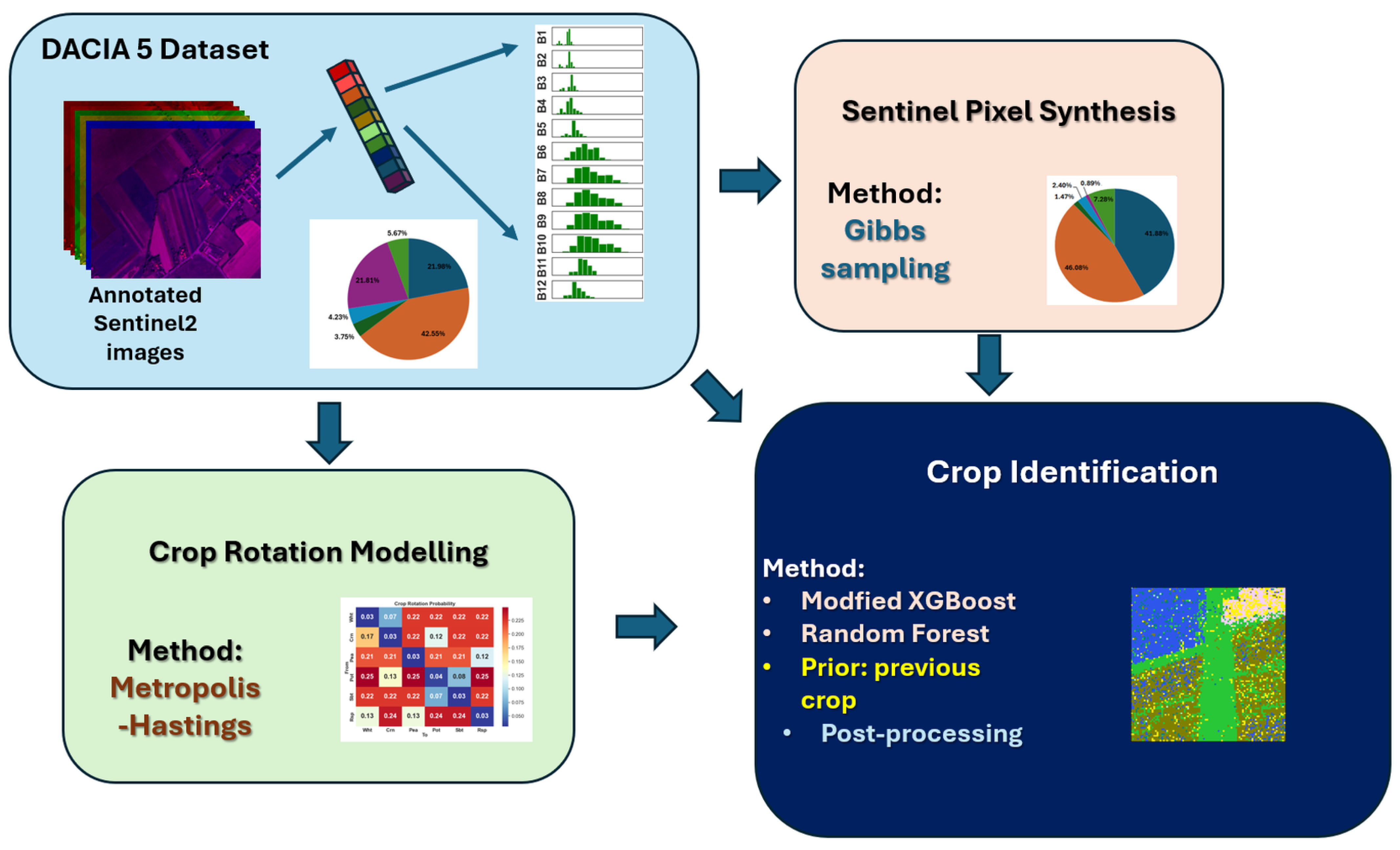
Figure 1. Overview of the work described in this paper. The original real-world data from the DACIA5 database is extrapolated, such that crop distribution can be adapted to any scenario, through pixel synthesis, using a modified Gibbs Sampling method. Simulated crop pixels are complemented by simulated previous crops generated using a crop rotation model. All data is, then, evaluated in a crop identification module.
Agriengineering 07 00259 g001
Figure 2. DACIA5 RGB-rendered images along with their shared mask.
Agriengineering 07 00259 g002
Figure 3. R 0 —The rotation model that was observed in DACIA 5 dataset. The model was used to improve the classification output and the results can be seen in results section.
Agriengineering 07 00259 g003
Figure 4. The relative distribution of six crop considered with respect to data from the Brașov area and, respectively, Romania overall. Changing the region, the relative probabilities changes, and thus, new pixels are needed.
Agriengineering 07 00259 g004
Figure 5. Histograms showing the distribution of pixel values for each crop class across all spectral bands.
Agriengineering 07 00259 g005
Figure 6. Mahalanobis distances to original pixels from original pixels and synthetic pixels.
Agriengineering 07 00259 g006
Figure 7. R 1 —A rotation model obtained after applying the formula (6) with α = 1.2. The model was used to improve the classification output and the results can be seen in Table 2, Table 3 and Table 4.
Agriengineering 07 00259 g007
Figure 8. R 2 —A rotation model obtained with more randomness. The model was used to improve the classification output and the results can be seen in Table 3 and Table 4.
Agriengineering 07 00259 g008
Figure 9. Classification output for different crop regions with and without rotation compared with the ground truth.
Agriengineering 07 00259 g009
Figure 10. The confusion matrix before rotation (left hand side) and after using the rotation model. The best solutions for testing on 2022 are shown.
Agriengineering 07 00259 g010
Table 1. Crop rotation difficulty scores representing the relative ease of rotating from one crop (indicated by the row) to another crop (indicated by the column). Each score reflects the tendency or suitability of a given crop rotation. A value of 1 denotes a highly favorable rotation practice, while 5 signifies a rotation that is less advisable.
ToWheatCornPeaPotatoSugar BeetRapeseed
From
Wheat541111
Corn251311
Pea115113
Potato131541
Sugar beet111451
Rapeseed313115
Table 2. Evaluation on 2022 data. The rotation models are R 0 (Figure 3) and R 1 (Figure 7).
ClassifierRotation ModelSyntheticAccuracy [%]
XGBNoNo56.06
XGBPost-R0No55.68
XGBPost-R1No63.06
XGB-lossdefaultNo58.54
XGB-lossdef + post-R1No64.15
XGB-lossdef + post-R1Yes66.61
RFNoNo55.12
RFPost-R0No55.36
RFPost-R1No63.26
Table 3. Evaluation on 2020 data. Rotation model R 1 is the one from Figure 7.
ClassifierRotation ModelSyntheticAccuracy [%]
XGBNoNo58.25
XGBPost-R1No61.90
XGBPost-R2No63.26
XGB-lossdefaultNo58.92
XGB-lossdef + post-R2No61.75
XGB-lossdef + post-R2Yes67.15
RFNoNo58.25
RFPost-R1No61.94
Table 5. DACIA5: RF cross-validation across crop years (2020–2024) under four classification scenarios. The first row uses only real observed pixels without crop rotation post-processing. The second row applies crop rotation constraints using the rotation probability matrix. The last two rows introduce synthetic data (e.g., generated or augmented) combined with real pixels, evaluated both without and with rotation constraints.
Setup/YearAccuracy [%]
2020 2021 2022 2023 2024
Real pixels (no rotation)58.2543.3855.1263.8928.80
Real pixels (with rotation)61.9445.1863.2662.5634.17
Disclaimer/Publisher’s Note: The statements, opinions and data contained in all publications are solely those of the individual author(s) and contributor(s) and not of MDPI and/or the editor(s). MDPI and/or the editor(s) disclaim responsibility for any injury to people or property resulting from any ideas, methods, instructions or products referred to in the content.