Using Sentinel-1 Time Series Data for the Delineation of Management Zones

Abstract

The characterization of soil attribute variability often requires dense sampling grids, which can be economically unfeasible. A possible solution is to perform targeted sampling based on previously collected data. The objective of this research was to develop a method for mapping soil attributes based on Management Zones (MZs) delineated from Sentinel-1 radar data. Sentinel-1 images were used to create time profiles of six indices based on VV (vertical–vertical) and VH (vertical–horizontal) backscatter in two agricultural fields. MZs were delineated by analyzing indices and VV/VH backscatter bands individually through two approaches: (1) fuzzy k-means clustering directly applied to the indices’ time series and (2) dimensionality reduction using deep-learning autoencoders followed by fuzzy k-means clustering. The best combination of index and MZ delineation approaches was compared with four soil attribute mapping methods: conventional (single composite sample), high-density uniform grid (one sample per hectare), rectangular cells (one composite sample per cell of 5 to 10 hectares), and random cells (one composite sample per cell of varying sizes). Leave-one-out cross-validation evaluated the performance of each sampling method. Results showed that combining the VV/VH index and autoencoders for MZ delineation provided more accurate soil attribute estimates, outperforming the conventional, random cells, and often the rectangular cell method. In conclusion, the proposed methodology presents scalability potential, as it does not require prior calibration and was validated on soil types commonly found across Brazil’s agricultural regions, making it suitable for integration into digital platforms for broader application in precision agriculture.

1. Introduction

Information regarding the spatial and temporal variability of soil attributes plays a crucial role in the development of effective soil management strategies. By examining these data, farmers can adopt the most suitable cultivars and plant population densities for each specific point within the production area. This, in turn, facilitates the precise determination of the required amounts of fertilizers and soil acidity correctives, not only to maximize financial returns but also to promote more sustainable production [1].

However, developing an effective strategy for collecting data to characterize the spatial and temporal variability of soil attributes is a complex and challenging task. Research has highlighted the importance of establishing dense sampling grids, with a minimum density of one sample per hectare, to adequately capture the variability of soil attributes [2,3,4]. Webster and Oliver [5] demonstrated that variograms used to infer soil attributes at unsampled points are unreliable when based on fewer than 100 data points, potentially leading to inaccurate estimates with significant margins of error. Therefore, grid sampling can provide a precise basis for variable rate application, but the costs and labor requirements, especially in extensive areas with high variability, suggest that other approaches may be more economical [6].

To understand the spatial and temporal variability of soil attributes without the need to establish dense sampling grids, studies have demonstrated the potential of using soil sensors or the crop itself as a ‘soil sensor’ [1]. Apparent soil electrical conductivity sensors, yield maps, and canopy reflectance indices can provide maps with different spatial and temporal variability patterns and be used to delineate homogeneous areas known as Management Zones (MZs) [7,8,9,10,11,12]. Within each MZ, a low variability of soil attributes is assumed, recommending the collection of a single composite sample. Based on specific levels of these attributes, targeted management practices for each MZ are established [1]. This strategy reduces soil sampling costs compared to dense sampling grids [13,14]. At the same time, it provides a better distribution of management practices (cultivars, plant density, fertilizers) compared to the conventional soil sampling method, in which only a single attribute level—and consequently, a single management strategy—is determined for the entire area.

Although the development of MZs through these methods represents an advancement in precision agriculture, their adoption among farmers remains limited. This limitation is largely due to difficulties in accessing reliable historical yield maps, electrical conductivity data, and multispectral satellite image time series with high temporal resolution. For example, yield maps have been available since the early 1990s, yet their adoption is still limited to only 5% to 25% of the total cultivated area in the United States for crops such as winter wheat, cotton, sorghum, and rice, and 45% for corn and soybean crops [15]. Apparent soil electrical conductivity presents itself as an attractive alternative because it can be quickly and easily measured for fields using electromagnetic induction instruments. However, this type of data collection strongly depends on specialized service providers for data acquisition and interpretation, whose availability varies across agricultural regions, complicating the implementation of this technology.

The use of multispectral optical images, freely available from orbital platforms such as Landsat-8 and Sentinel-2, enables remote service delivery and extensive spatial coverage. However, its application faces significant challenges, such as cloud cover, which compromises consistent data acquisition. This issue is particularly critical in tropical regions, where average annual cloud cover can reach approximately 66%, hindering the construction of representative historical time series [16,17]. Therefore, to expand farmers’ adoption of MZs, it is essential to develop alternative methods capable of efficiently characterizing the spatial and temporal variability of soil attributes, with a lower cost per unit area and broader spatial coverage.

A promising line of research for characterizing the spatial and temporal variability of soil attributes through MZs is the use of Synthetic Aperture Radar (SAR) data. The Sentinel-1 mission, part of the European Union’s Copernicus program, currently consisting of the Sentinel-1A sensor, freely provides SAR imagery with a spatial resolution of 20 × 22 m and a temporal resolution of 12 days [18]. Equipped with an active C-band SAR sensor operating at a central frequency of 5.405 GHz with dual polarization (vertical–vertical and vertical–horizontal), this satellite can penetrate cloud cover and acquire imagery both day and night [19,20,21,22]. Moreover, its electromagnetic waves, characterized by a longer wavelength, can penetrate the superficial vegetation layers and, in some cases, reach deeper soil layers. In areas without vegetation cover, wave penetration into the soil makes SAR data sensitive to both the dielectric properties (such as soil moisture) and geometric characteristics (such as surface roughness) of the soil [23,24]. In agricultural contexts, SAR backscatter data have been used, either alone or in combination with multispectral data, for various applications, including soil moisture estimation [25,26,27], the assessment of soil physical properties [28,29,30,31], and the estimation of multispectral indices such as the Normalized Difference Vegetation Index (NDVI) [32,33,34], among other applications.

Therefore, the previously mentioned properties highlight the potential of Sentinel-1 SAR imagery as a rich source of spatiotemporal information, making it promising for estimating soil attributes through the delineation of MZs. A methodology can be applied to create temporal profiles of backscatter with dual polarization—VV (vertical–vertical) and VH (vertical–horizontal)—from SAR data, complemented by the calculation of specific SAR indices. These temporal profiles can be analyzed using unsupervised classification techniques to identify regions with similar backscatter responses, potentially associated with variations in soil attributes. Although the fuzzy clustering of time series of vegetation indices, such as NDVI, has been widely used for the delineation of MZs, this study introduces two main innovations: (i) the application of autoencoders for compressing SAR time series and (ii) the direct comparison of different sampling strategies, including conventional methods (a single composite sample), rectangular cell-based methods ranging from 5 to 10 ha (a composite sample per cell), and random cells with varying sizes and shapes. Thus, the objective of this study was to develop a method for mapping soil attributes through the delineation of MZs using SAR data provided by Sentinel-1.

2. Materials and Methods

2.1. Field of Study

This study was conducted in two commercial grain production fields (Field A and Field B) that exhibit different soil texture characteristics (Figure 1). Field A covers an area of 117 hectares and is situated in the municipality of Sinop, Mato Grosso, Brazil (11°8′20″ S and 56°19′18″ W). Field B spans an area of 106 hectares and is situated in the municipality of Chapadão do Céu, Goiás, Brazil (18°20′10″ S and 52°37′12″ W). According to the Brazilian Soil Classification System, Field A is identified as a Dystrophic Red–Yellow Latosol, while Field B is classified as a Dystrophic Red Latosol [35]. Latosols constitute the most geographically widespread soil group in Brazil, especially in tropical regions such as the Cerrado [36]. Both areas were selected due to their high variability in attributes, especially physical ones such as Clay content, making them ideal for evaluating methodologies aimed at mapping spatial variability. Additionally, as they are located in the Brazilian Cerrado, one of the country’s main grain-producing regions, these areas provide a favorable context for extrapolating the scalability and applicability of the proposed methodology. For soil sampling, a grid-point sampling method was adopted with an approximate spacing of 100 m. Field A was represented by 113 samples, and Field B was represented by 104 samples. The values of 9 soil attributes were determined in the laboratory from the grid of points established in each field. Descriptive statistics of these attributes are summarized in

Table 1. Summary of descriptive statistics of soil properties measured in the study area.

Field	Soil Attribute	Unity	Mean	Minimum	Maximum	STD	CV (%)
A	CLA	%	35.65	16.30	62.00	11.91	33
	pH	-	6.11	5.76	7.78	0.28	5
	P	mg/dm3	17.91	3.40	56.60	10.40	58
	K+	mg/dm3	86.24	25.00	199.00	36.72	43
	Ca2+	cmolc/dm3	2.55	0.99	5.82	0.70	28
	Mg2+	cmolc/dm3	0.84	0.43	1.68	0.22	26
	C	cmolc/dm3	1.43	0.47	2.78	0.45	31
	V	%	51.65	36.70	97.00	8.95	17
	H+ + Al3+	cmolc/dm3	3.28	0.20	5.20	0.81	25
B	CLA	%	37.00	19.00	58.30	7.71	21
	pH	-	6.35	5.81	6.91	0.21	3
	P	mg/dm3	13.75	2.50	30.10	6.16	45
	K+	mg/dm3	55.55	26.0	120.00	19.43	35
	Ca2+	cmolc/dm3	3.30	2.14	5.23	0.61	18
	Mg2+	cmolc/dm3	1.25	0.72	2.08	0.29	24
	C	cmolc/dm3	1.58	0.87	2.86	0.32	2
	V	%	62.29	49.50	74.60	5.46	9
	H+ + Al3+	cmolc/dm3	2.87	1.20	4.40	0.72	25

CLA: Clay; pH: Active Acidity in water; P: Phosphorus; K⁺: Potassium; Ca²⁺: Calcium; Mg²⁺: Magnesium; C: Soil Organic Carbon; V: Basis Saturations; H⁺ + Al³⁺: potential acidity; STD: standard deviation; CV: coefficient of variation (%).

.

2.2. Sentinel-1 Dataset and Preprocessing

The SAR data used in this study were freely obtained from the Sentinel-1A sensor of the European Union’s Copernicus program. The Sentinel-1 mission provides global SAR data in the C-band (central frequency of 5.405 GHz) with dual polarization (VV and VH). The temporal resolution is 12 days, although it can be higher in some cases due to overlapping sensor passes. In this study, the Sentinel-1 collection available on Google Earth Engine was used, comprising Ground Range Detected (GRD) format images processed with the Sentinel-1 toolbox to produce calibrated and orthorectified products. All images were acquired in descending orbits using the Interferometric Wide (IW) swath mode and dual polarization (VV and VH). They have a pixel spacing of 10 m but a spatial resolution of 20 × 22 m [18].

The preprocessing steps for the SAR data included border noise removal, speckle filtering, terrain radiometric normalization, and the conversion of the backscatter coefficient to decibels. Image border noise results from the process of converting acquisitions from GRD format to IW, and its presence is an undesired processing artifact that limits its full exploitation in various applications [37]. The speckle phenomenon, common in SAR images due to the interference of radar waves reflected by surfaces smaller than the radar resolution, was addressed through multitemporal filtering [38]. The Refined Lee filter, 3 × 3 [39], was used with a multitemporal filtering structure of 10 images. Terrain radiometric normalization corrects variations in the received signal due to terrain slope. For this, the Shuttle Radar Topography Mission digital elevation model with a 1 arc-second resolution (~30 m) [40] was employed, deriving elevation, slope, and aspect values for normalization. Finally, as the last preprocessing step, the terrain-corrected radiometric backscatter coefficient was converted to decibels through a logarithmic transformation.

Table 2. Specifications of the Sentinel-1 SAR data used in this study.

Parameters	Specifications
Satellite Pass	Descending
Polarization	Vertical–Vertical (VV) Vertical–Horizontal (VH)
Speckle Filter	Refined Lee—3 × 3 [43]
Speckle Filter Framework	Multitemporal—10 images
Digital Elevation Model	NASA SRTM Digital Elevation 30 m [44]

SRTM: Shuttle radar topography mission.

summarizes the parameters and specifications for image acquisition and preprocessing. The data were preprocessed using Google Earth Engine (GEE) [41]. All GEE codes for Sentinel-1 data preprocessing were provided by Mullissa et al. [42] and are available at https://github.com/adugnag/gee_s1_ard (accessed on 7 August 2023).

2.3. Generation of Temporal Profiles and SAR Indices

After preprocessing, each SAR image was converted into a dataframe and stored to generate temporal backscatter profiles. For each analyzed field, a grid of 40 m × 40 m quadrilaterals was established. In each image, the average pixel values within these quadrilaterals were calculated, thereby constructing the temporal backscatter profiles for the VV and VH bands. This method helps minimize the potential residual noise in the images and reduces the computational load required for subsequent analyses. Based on these profiles, six indices were calculated using Sentinel-1 data, as detailed in

Table 3. The SAR (Synthetic Aperture Radar) indices used in this study to delineate Management Zones.

Full Name	Abbreviated Name	Equation	Source
Polarimetric Radar Vegetation Index	PRVI	$\left(1-{\displaystyle \frac{VV}{VH+VV}}\right)\times VH$	[43]
Sentinel-1 Radar Vegetation Index	RVI4S1	$\sqrt{{\displaystyle \frac{VV}{VH+VV}}}\times {\displaystyle \frac{4\times VH}{VH+VV}}$	https://custom-scripts.sentinel-hub.com/custom-scripts/sentinel-1/radar_vegetation_index/# (accessed on 15 September 2023).
Radar Vegetation Index	RVI	${\displaystyle \frac{4\times VH}{VH+VV}}$	[44]
Normalized Ratio Procedure Between Bands	NRPB	${\displaystyle \frac{VH-VV}{VH+VV}}$	[45]
VV VH Ratio	VV/VH	${\displaystyle \frac{VV}{VH}}$	[34]
VH VV Ratio	VH/VV	${\displaystyle \frac{VH}{VV}}$	[32]
VH Backscattering	VH	$VH$	-
VV Backscattering	VV	$VV$	-

VV: Vertical–vertical polarization; VH: vertical–horizonal polarization.

. Each VV and VH temporal backscatter series, as well as the indices for each quadrilateral, was standardized using z-score normalization. This process adjusts the data so that each set has a mean of 0 and a standard deviation of 1. To avoid issues of collinearity among the indices, Pearson correlation (r) was calculated between them. Based on this analysis, only those indices that showed lower collinearity (r < 0.95) were included, thus ensuring the independence and relevance of each chosen index for the definition of MZs.

To understand the seasonal variability of the SAR indices, rainfall data from the NASA-POWER system (https://power.larc.nasa.gov, accessed on 22 August 2023) were used, considering that radar data are sensitive to soil moisture [25,26,27]. This system was developed to provide meteorological information directly applicable to fields such as architecture, energy generation, and agrometeorology. It compiles information from various data sources, including grid-derived data, to offer a comprehensive view of climate and weather conditions [46].

2.4. Delineation of Management Zones Using SAR Data

To delineate the MZs, all SAR indices were analyzed individually, and two approaches were proposed. The first approach (Approach 1) involved the direct application of the fuzzy k-means clustering algorithm [47] on the temporal series of the SAR indices. In the second approach (Approach 2), a machine learning method known as autoencoders was implemented to reduce the dimensionality of the temporal series. Autoencoders are a type of neural network often used in unsupervised machine learning tasks, such as feature extraction [48]. The basic architecture of an autoencoder is divided into three parts: encoder, bottleneck layer, and decoder. The encoder receives the input data (in this case, SAR indices) and compresses it into a lower-dimensional representation (bottleneck layer). The decoder then takes this compressed representation and attempts to reconstruct the original data from it. This process is carried out during the training of the autoencoder network. Thus, after training, the bottleneck layer was used as input to the fuzzy k-means algorithm to cluster the SAR data time series and, consequently, define the MZs.

To define the architecture and training parameters, a k-fold cross-validation procedure, with k = 5, was implemented to identify the most suitable hyperparameters and to prevent overfitting by ensuring the model’s generalization across different data subsets. The selection of the final model was based on the lowest mean squared error obtained during the validation process. The selected architecture and training parameters are detailed in

Table 4. A proposed autoencoder architecture for feature extraction.

Layers	Type	Neurons	Activation Function
Input Layer (SAR)	-	Number of SAR images in each field	-
Encoder Layer 1	Fully Connected	32	ReLU
Bottleneck Layer 1	Fully Connected	6	ReLU
Decoder Layer 1	Fully Connected	32	ReLU
Output Layer	Fully Connected	Number of SAR images in each field	Linear

ReLU: Rectified Linear Unit; SAR: Synthetic Aperture Radar.

and

Table 5. Parameters used to train the autoencoder architecture.

Parameter	Value
Number of Epochs	200
Optimization Function	Adam
Learning Rate	0.0001
Batch Size	1
Loss Function	Mean Squared Error
Regularization	L2 (lambda = 0.01)

. The ReLU activation function (σ(x) = max(0, x)) was used in the hidden layers due to its computational simplicity and the advantages it offers in terms of training convergence and stability [49]. In the output layer, a linear activation function (σ(x) = x) was applied to allow the reconstruction of the time series normalized by the z-score, which may include both negative and positive values. A linear activation was applied in the output layer to allow the reconstruction of values normalized by the z-score, which can take both negative and positive values. Figure 2 presents the loss curves during the training and validation processes, expressed as root mean square error (RMSE), over 200 epochs. The progressive reduction in loss values, followed by stabilization, indicates that the autoencoder effectively minimized the reconstruction error without signs of overfitting. These results demonstrate the generalization capability of the selected architecture and the adequacy of the defined training parameters.

The simulations were conducted considering the number of clusters, in this case MZs, equal to three for both approaches and fields. After clustering, QGIS geoprocessing tools were used for refinements. Clusters with an area smaller than 3 hectares were integrated into the larger contiguous clusters, while clusters larger than 3 hectares but geographically disconnected and sharing the same label were considered as distinct clusters.

2.5. Validation of Management Zones Generated Using SAR Data

The most common soil sampling methods include the conventional soil sampling method (CONV), the cell-based soil sampling method (CEL), the uniform grid soil sampling method (GRID-1), and the MZ-based soil sampling method. The CONV method involves collecting several samples to form a single composite sample, which is considered representative of the entire field. In the present study, the CONV method was considered the average of all the collected samples. The CEL method, on the other hand, divided the area into cells (polygons of 5 to 10 hectares), ensuring the presence of at least four GRID-1 samples in each cell. The attribute estimation in each cell was the average of the samples collected within each cell. A fifth comparison method was proposed, where cells are created randomly, called the random cell-based soil sampling method (CEL-RND) (Figure 3). The number of random cells was defined to match the number of MZs established by the SAR data-based method. In total, 1000 random cell scenarios were generated for each study area. The minimum size of each random cell was 4 hectares to ensure the presence of at least four soil samples per cell. The random cells were generated using a Python script (version 3.10) based on Voronoi Diagrams, proposed by Georgy Voronoi [50], and the soil attributes within each cell were estimated by the average of the samples collected within each cell.

2.6. Evaluation of Sampling Methods

To evaluate the performance of each sampling method, the ‘leave-one-out’ cross-validation (LOOCV) method was used, always based on the GRID-1 data. In this way, we ensured the participation of all the points in the error calculation for all the evaluated methods. In LOOCV, each point from the GRID-1 dataset was successively removed, and its estimate was made using the sampling methods: CONV, CEL, MZ, GRID-1, and CEL-RND. After the estimation, the point was reintegrated into the dataset. This process continued until all the GRID-1 points were evaluated. For the CONV, the estimate of the removed point was calculated from the average of the remaining points. For the CEL, MZ, and CEL-RND methods, the estimate was based on the average of the remaining samples within their respective areas. Finally, to evaluate the GRID-1 method, the estimate of the removed point was a value interpolated using ordinary kriging based on the fitting of semivariograms. Semivariograms are tools that allow for the characterization and determination of distribution patterns, such as randomness, uniformity, and spatial trends [51]. For this, Equation (1) was used to calculate the semivariance:

$${\gamma }^{*}\left(h\right)={\displaystyle \frac{1}{2N\left(h\right)}}{\sum }_{i=1}^{N\left(h\right)}{(z\left(x_i\right)-z(x_i+h\left)\right)}^2$$

(1)

where ${\gamma }^{*}\left(h\right)$ is the value of the experimental semivariance at the distance interval h; $z\left(x_i\right)$ is the sample value measured at the sampling points $x_i$, where data exist at $x_i$ and $x_i+h$; and $N\left(h\right)$ is the total number of sample pairs within the distance interval h.

During the adaptation of theoretical models to the experimental semivariograms, coefficients were determined that describe the nugget effect (C0), sill (C0 + Cp), partial sill (Cp), and range (A). The models tested for adaptation included the spherical, exponential, Gaussian, and linear models, and they were selected based on maximizing the coefficient of determination (R²), minimizing the sum of squared residuals, and maximizing the correlation coefficient obtained through cross-validation. These metrics are used to evaluate how well the fitted model matches the experimental data. The Spatial Dependence Index (SDI) was analyzed using the ratio C0/(C0 + Cp), and the intervals proposed by [52] were employed to classify spatial dependence into three categories: strong dependence (SDI < 25%), moderate dependence (25% ≤ SDI < 75%), and weak dependence (SDI ≥ 75%). Semivariograms of soil chemical and physical attributes were modeled using SmartMap [53] Version 1.4, an open-source plugin developed for QGIS.

By comparing the estimated values of soil attributes obtained by the CONV, CEL, MZ, GRID-1, and CEL-RND methods with the sampled values at each corresponding point, the root mean square error (RMSE) was calculated. This analysis was conducted individually for each study field, following the methodology established in Equation (2):

$$\mathrm{R}\mathrm{M}\mathrm{S}\mathrm{E}= \sqrt{{\displaystyle \frac{1}{n}} {\sum }_{i=1}^n{(x_i-\widehat{x_i})}^2}$$

(2)

where $\widehat{x_i}$ represents the estimated value of the soil attribute at point $i$, $x_i$ is the observed value of the soil attribute at point $i$ and $n$ is the number of sampled points.

To compare the MZs defined from the SAR data with the other soil sampling methods used in this study, the combination of Approach 1 or 2 and the SAR index that resulted in the lowest RMSE was selected. After this selection, the average of each attribute was calculated for each zone, and then the attributes were compared using the F-test (with a significance level of p-value < 0.05). The RMSE values of the MZ sampling method for each field were compared with the other values resulting from the sampling methods evaluated in this study. To evaluate the CEL-RND method, we quantified, across 1000 generated scenarios, the frequency with which the MZ method showed a higher RMSE than CEL-RND. Then, the percentage of these scenarios in which the MZ method performed worse, in terms of RMSE, compared to the CEL-RND method was calculated.

3. Results

3.1. Exploratory Analysis of the SAR Dataset

Between 1 January 2018 and 31 March 2023, 319 images were obtained for Field A and 266 images were obtained for Field B, resulting in average temporal resolutions of 6.0 and 7.4 days, respectively. Figure 4 shows the Pearson correlation estimated between the VV and VH backscatter values and the SAR indices. The correlations obtained were found to be significant, with p-values equal to zero. The indices RVI, NRPB, VH/VV, and VV/VH showed high r with each other, as well as PRVI and VH, exhibiting values above 0.95. On the other hand, the RVI4SI index showed the lowest level of r with the other indices. Based on these results, four indices (VV, VH, VV/VH, RVI4SI) were selected for the continuation of the study.

The monthly averages of the time series for the VV and VH backscatter coefficients, as well as the VV/VH and RVI4SI indices, were plotted for both fields in each year (Figure 5). Considering that the data availability extended only until March 2023, the graphical analysis was restricted to the period from 2018 to 2022. The time series of the calculated indices exhibited seasonal trends. Except for the VV/VH index, an increase was observed between September and December, followed by a decline in February. This behavior coincides with the period of increased monthly accumulated precipitation (Figure 6), suggesting a possible relationship between higher soil moisture or vegetation growth and elevated backscatter levels. From February to March, although precipitation tends to remain relatively constant, there is a new increase in backscatter, likely due to the growth of second-crop vegetation. Subsequently, from May to September, there was a decrease in the SAR indices, in line with the reduction in monthly accumulated precipitation and crop biomass. For the VV/VH index, there was an increase between January and February, which then gave way to a decrease from February to April, except for the years 2019 and 2021. Additionally, only for the VV/VH index, an increase in values was recorded from April to August.

3.2. Analysis of Spatial Variability in Soil

The analysis of the experimental semivariograms in GRID-1 confirmed the spatial variability of the soil attributes for both fields (

Table 6. The theoretical model parameters are adjusted to the empirical semivariance of the soil attributes for Field A and Field B.

Field	Soil Attribute	Model	Range (m)	C0	C0 + C	R2	SDI (%)
A	CLA	Gaussian	697.85	14.72	198.50	0.99	7.42
	pH	Linear to Sill	370.64	0.022	0.036	0.47	61.11
	P	Spherical	396.95	45.27	96.66	0.74	46.83
	K+	Linear to Sill	642.51	286.77	1012.68	0.99	28.32
	Ca2+	Linear to Sill	419.14	0.12	0.36	0.79	33.33
	Mg2+	Linear to Sill	458.12	0.02	0.04	0.83	50.00
	C	Linear to Sill	472.85	0.04	0.17	0.97	23,52
	V (%)	Linear to Sill	347.48	28.78	48.47	0.59	59.37
	H+ + Al3+	Linear to Sill	379.13	0.24	0.57	0.67	42.11
B	CLA	Spherical	401.31	3.77	58.51	0.97	6.44
	pH	Linear	557.85	0.02	0.04	0.948	50.00
	P	Linear to Sill	320.92	26.97	33.60	0.29	80.26
	K+	Exponential	788.23	160.36	341.29	0.92	46.99
	Ca2+	Linear	552.69	0.13	0.30	0.98	43.33
	Mg2+	Linear	559.91	0.03	0.08	0.99	37.50
	C	Linear	557.18	0.03	0.09	0.99	33.33
	V	Linear to Sill	585.78	23.10	31.00	0.96	74.19
	H+ + Al3+	Linear	569.48	0.09	0.53	0.98	16.98

CLA: Clay (%); pH: Active Acidity in water; P: Phosphorus (mg dm⁻³); K⁺: Potassium (mg dm⁻³); Ca²⁺: Calcium (cmolc dm⁻³); Mg²⁺: Magnesium (cmolc dm⁻³); C: Soil Organic Carbon (cmolc dm⁻³); V: Basis Saturations (%); H⁺ + Al³⁺: potential acidity (cmolc dm⁻³); range (m); C0: nugget effect; C0 + C: sill; R²: coefficient of determination; SDI (%): Special Dependency Index.

). When analyzing the SDI, it was found that Clay (CLA) content and Soil Organic Carbon (C) in Field A and CLA and potential acidity (H⁺ + Al³⁺) in Field B had SDI values lower than 25%, indicating a high spatial dependence [52]. All other elements, except for Phosphorus (P) in both fields, exhibited SDI values between 25% and 75%, which indicates moderate spatial dependence. Figure 7 and Figure 8 show the maps constructed using ordinary kriging after semivariogram fitting. In Fields A and B, the maps of CLA and C, as well as those of Ca²⁺ and Magnesium (Mg²⁺), respectively, display visual similarities that indicate high correlations between these soil attributes.

3.3. Delineation of Management Zones with SAR

Regarding the design and quantity of MZs, visual variations were observed depending on the SAR index used and the methodology adopted (Figure 9). These variations in size, shape, and number of MZs became even more noticeable when contrasting the proposed methodologies. The total number of MZs in Approach 2 exceeded that of Approach 1. In the case of Field B, the number of MZs according to Approach 1 was two, lower than the initially stipulated value of three. This result is because some clusters created by the Fuzzy C-means algorithm did not have significant associations with data points or exhibited an extremely low degree of membership in relation to all points for a specific cluster. Additionally, the RVI4SI index resulted in excessively fragmented clusters compared to the other algorithms evaluated. Due to this fragmentation, it was considered inappropriate to use this index for the creation of MZs in Field B. Therefore, its results were not considered in this study.

Table 7. RMSE of Approaches 1 and 2 for Fields A and B related to the VV and VH backscatter coefficients and the SAR indices VV/VH and RVI. Bold indicates the lowest unique RMSE values.

Field	Approach	Soil Attribute	VV	VH	VV/VH	RVI4SI
A	1	CLA	8.99	9.01	7.82	7.67
		pH	0.27	0.27	0.27	0.27
		P	10.08	10.18	9.74	9.42
		K+	31.63	31.73	29.73	29.21
		Ca2+	0.66	0.65	0.65	0.65
		Mg2+	0.20	0.20	0.19	0.20
		C	0.38	0.38	0.36	0.35
		V	8.99	8.93	9.04	9.09
		H+ + Al3+	0.82	0.83	0.81	0.80
	2	CLA	8.33	6.34	5.74	7.82
		pH	0.27	0.27	0.27	0.27
		P	9.98	9.81	9.67	10.02
		K+	31.28	24.87	23.7	29.47
		Ca2+	0.65	0.64	0.64	0.63
		Mg2+	0.19	0.19	0.19	0.19
		C	0.36	0.30	0.27	0.35
		V	9	9.08	9.05	8.99
		H+ + Al3+	0.82	0.75	0.75	0.83
B	1	CLA	7.77	7.81	7.48	-
		pH	0.21	0.21	0.19	-
		P	6.24	6.23	6.21	-
		K+	19.24	18.79	18.28	-
		Ca2+	0.61	0.6	0.55	-
		Mg2+	0.29	0.29	0.26	-
		C	0.32	0.31	0.29	-
		V	5.51	5.52	5.30	-
		H+ + Al3+	0.70	0.70	0.56	-
	2	CLA	7.31	7.8	6.53	-
		pH	0.19	0.19	0.2	-
		P	6.14	6.26	6.08	-
		K+	18.25	19.03	19.22	-
		Ca2+	0.57	0.57	0.53	-
		Mg2+	0.27	0.27	0.25	-
		C	0.29	0.29	0.28	-
		V	5.31	5.31	5.52	-
		H+ + Al3+	0.58	0.59	0.58	-

CLA: Clay (%); pH: Active Acidity in water; P: Phosphorus (mg dm⁻³); K⁺: Potassium (mg dm⁻³); Ca²⁺: Calcium (cmolc dm⁻³); Mg²⁺: Magnesium (cmolc dm⁻³); C: Soil Organic Carbon (cmolc dm⁻³); V: Basis Saturations (%); H⁺ + Al³⁺: potential acidity (cmolc dm⁻³); VV: vertical–vertical polarization; VH: vertical–horizonal polarization; VV/VH: VV VH ratio: RVI4SI: Sentinel-1 Radar Vegetation Index.

presents the RMSE obtained through LOOCV, representing the accuracy of the soil attribute estimates for Fields A and B using Approaches 1 and 2 with the MZ method. In the evaluation of errors associated with soil attribute estimation, the VV/VH index consistently stood out, achieving the lowest RMSE values compared to the other indices. For example, in Field A, when estimating the Clay content attribute using Approach 2, the VV backscatter band recorded an RMSE of 8.33, while the VV/VH index showed a significantly lower RMSE of 5.74. When analyzing the two approaches, it is observed that Approach 2 has an advantage in terms of accuracy over Approach 1, especially when adopting the VV/VH ratio for soil attribute estimation. In all fields studied, the attributes CLA, P, Ca^2+, and C recorded a lower RMSE with Approach 2 when using the VV/VH index.

The results indicated significant differences in soil attribute values between the MZs delineated by Approach 2 and the SAR index VV/VH, which had the lowest RMSE (

Table 8. Univariate analysis of variance of soil attributes for the Management Zones delineated by Approach 2 and the SAR VV/VH index for fields A and B.

Field	Management Zones	Number of Samples	Soil Attributes
			CLA	pH	P	K	Ca2+	Mg2+	C	V	H+ + Al3+
A	MZ1	20	38.11	6.29	19.81	73.35	2.91	0.87	1.47	54.40	3.34
	MZ2	52	25.97	6.02	21.41	67.38	2.20	0.72	1.12	49.84	3.04
	MZ3	12	58.23	6.05	8.48	160.50	3.11	1.09	2.29	50.03	4.33
	MZ4	28	42.18	6.15	14.13	98.64	2.70	0.93	1.59	53.75	3.23
	Variance analysis	F-Value	128.50	5.25	7.98	57.93	11.57	17.78	69.34	2.03	10.15
		Prob > F	0	0	0	0	0	0	0	0.11	0
B	MZ1	49	39.30	6.26	14.54	62.08	3.60	1.41	1.73	60.94	3.31
	MZ2	4	40.58	6.28	16.7	55.00	3.80	1.54	1.75	63.32	3.18
	MZ3	14	33.75	6.42	14.61	52.5	3.16	1.15	1.48	63.9	2.56
	MZ4	20	40.58	6.42	9.63	48.85	2.98	1.06	1.44	62.92	2.45
	MZ5	17	28.01	6.51	14.92	47.24	2.81	1.03	1.33	63.91	2.25
	Variance analysis	F-Value	12.80	6.89	3.13	3.07	11.21	13.86	9.14	1.57	16.57
		Prob > F	0	0	0.02	0.02	0	0	0	0.19	0

CLA: Clay (%); pH: Active Acidity in water; P: Phosphorus (mg dm⁻³); K⁺: Potassium (mg dm⁻³); Ca²⁺: Calcium (cmolc dm⁻³); Mg²⁺: Magnesium (cmolc dm⁻³); C: Soil Organic Carbon (cmolc dm⁻³); V: Basis Saturations (%); H⁺ + Al³⁺: potential acidity (cmolc dm⁻³).

). At least one mean of each soil attribute from the MZs differed statistically at a p-value < 0.05, except for the V attribute in both fields. For Field A, MZ₃ was characterized as the zone with the highest average values of CLA, Potassium (K⁺), Ca²⁺, Mg²⁺, C, and potential acidity (H⁺ + Al³⁺), while MZ₂ had the lowest values. For Field B, MZ₂ was characterized as the zone with the lowest average values of CLA, P, Ca²⁺, Mg²⁺, and C.

Figure 10 presents a comparison between the error (RMSE) obtained by the MZ method using Approach 2 and the SAR index VV/VH and the error generated from 1000 different CEL-RND scenarios. The value indicated on each bar represents the percentage of times the MZ method, based on SAR data, had a higher error than the random cell method. Therefore, the lower the percentage value displayed on the bar, the better the performance of the MZ method compared to CEL-RND. Values equal to or greater than 50% indicate that MZs do not contribute to the representativeness of the soil attribute variability compared to a random process. As can be observed, for most soil attributes in both fields, the RMSE resulting from the CEL-RND sampling method was higher than the RMSE obtained by the MZ sampling method, resulting in values below 50%. In Field A, the attributes with the lowest percentage of errors (less than 5%) were CLA, K⁺, C, H⁺ + Al³⁺, and pH. This indicates that the MZ method performed well for these attributes in this field. The V attribute, on the other hand, showed a significantly higher error percentage of 43%, indicating that the MZ method may not be as efficient for this specific attribute. In Field B, the CLA attribute had a relatively low error percentage, around 3.9%. On the other hand, pH, K⁺, and V showed considerably higher errors, around 48%, 72%, and 77%, respectively.

3.4. Comparing Soil Sampling Methods

Table 9. RMSEs of the sampling methods GRID-1, CONV, CEL, and MZs delineated by Approach 2 and the SAR index VV/VH for soil attributes in Fields A and B. Bold indicates the lowest unique RMSE values.

Field	Soil Attribute	GRID-1	CONV	CEL	MZs
A	CLA	3.49	11.97	6.24	5.74
	pH	0.22	0.28	0.29	0.27
	P	6.72	10.44	10.23	9.67
	K	18.59	36.88	25.32	23.7
	Ca2+	0.43	0.71	0.64	0.64
	Mg2+	0.15	0.22	0.2	0.19
	C	0.17	0.45	0.31	0.27
	V	7.07	8.99	9.34	9.05
	H+ + Al3+	0.55	0.82	0.84	0.75
B	CLA	1.45	7.75	6.35	6.53
	pH	0.14	0.21	0.2	0.2
	P	5.24	6.19	6.95	6.08
	K	12.69	19.52	20.12	19.22
	Ca2+	0.36	0.61	0.46	0.53
	Mg2+	0.14	0.3	0.2	0.25
	C	0.19	0.32	0.26	0.28
	V	4.63	5.48	5.66	5.52
	H+ + Al3+	0.26	0.72	0.54	0.58

CLA: Clay (%); pH: Active Acidity in water; P: Phosphorus (mg dm⁻³); K⁺: Potassium (mg dm⁻³); Ca²⁺: Calcium (cmolc dm⁻³); Mg²⁺: Magnesium (cmolc dm⁻³); C: Soil Organic Carbon (cmolc dm⁻³); V: Basis Saturations (%); H⁺ + Al³⁺: potential acidity (cmolc dm⁻³). GRID-1: uniform grid soil sampling method; CONV: conventional soil sampling method; CEL: cell soil sampling method; MZ: Management Zone soil sampling method.

highlights the RMSE obtained through LOOCV cross-validation, demonstrating the accuracy of the soil attribute estimates in Fields A and B using different sampling strategies: GRID-1, CONV, CEL, and MZs using Approach 2 and the SAR index VV/VH. The GRID-1 method recorded the lowest RMSE values in both fields, indicating superiority in the precision of soil attribute estimates. In both fields, the CONV method stood out with the highest RMSE values, indicating lower precision in soil attribute estimates. The MZs delineated from the SAR data showed superiority compared to the CONV and CEL methods in Field A. In Field B, MZs outperformed the conventional method.

4. Discussion

In the context of remote sensing applied to agricultural fields dedicated to grain production, SAR backscatter time series were used in this study to delineate MZs. Although the Sentinel-1 satellite has a nominal temporal resolution of 12 days for South America, a shorter revisit interval was observed, possibly due to the overlapping of imaging swaths during consecutive satellite passes. Previous studies have demonstrated that higher temporal resolution enhances trend detection and the identification of spatiotemporal patterns related to crop phenology [54]. Moran et al. [55] pointed out that, in the case of C-band SAR data, temporal resolutions between 3 and 6 days are more suitable for distinguishing crop types and monitoring their phenology, while daily monitoring is necessary to capture the rapid changes in soil moisture conditions. Therefore, the higher temporal resolution observed provides improved conditions for understanding and interpreting variations in backscatter over time, potentially contributing to a more accurate delineation of MZs and greater accuracy in estimating soil attributes.

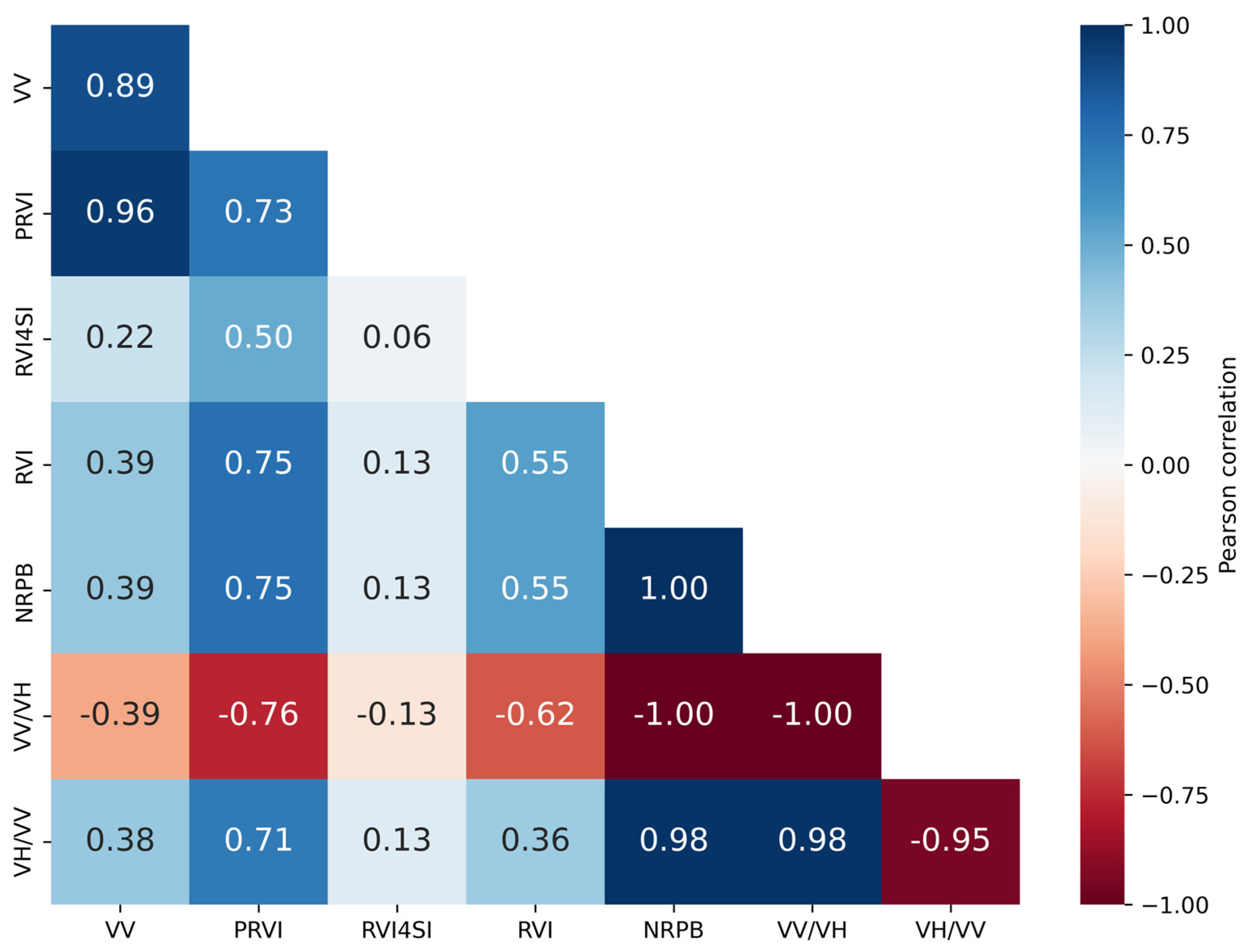
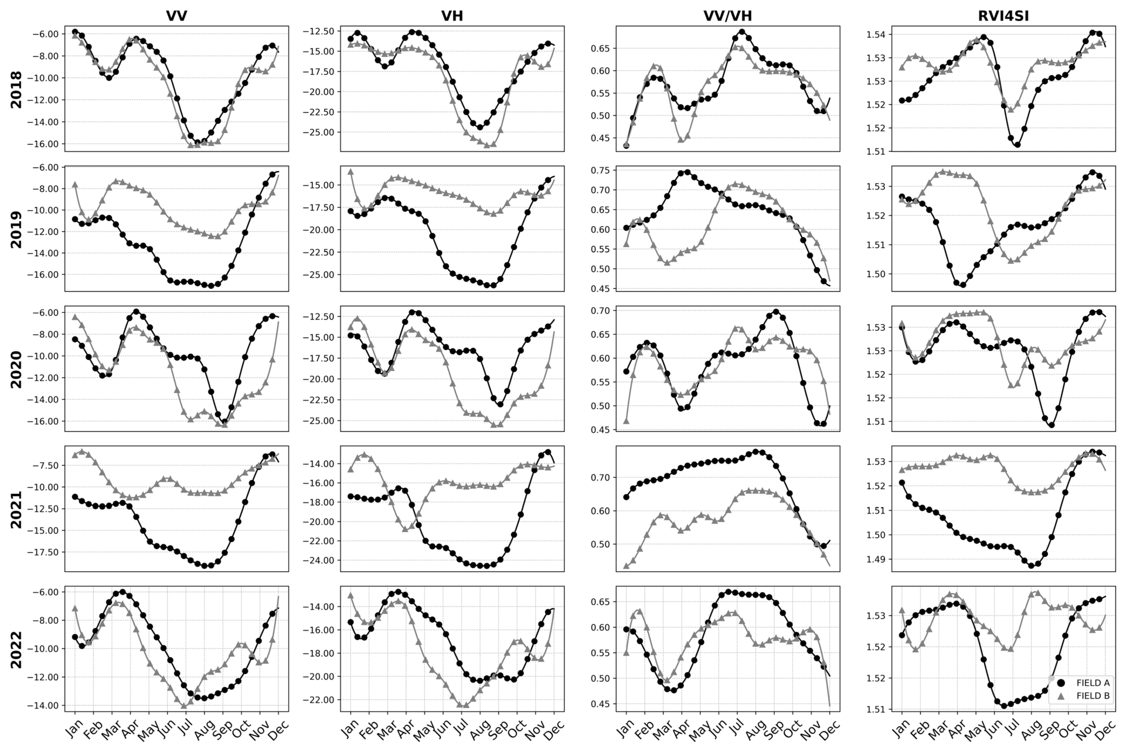
The analysis of the relationship between VV and VH backscatter values and SAR indices revealed that certain indices exhibit strong correlations, indicating potential redundancies. This finding aligns with the study by [56], which identified that the RVI, NRPB, VH/VV, and VV/VH indices show high mutual correlation, with values greater than 0.95 or less than −0.95. Additionally, in both our analysis and the cited study, the RVI4SI index displayed the lowest correlation compared to other indices. Therefore, these findings suggest that, regardless of the agricultural fields studied, the relationship between VV and VH backscatter values and SAR indices tends to follow similar patterns.

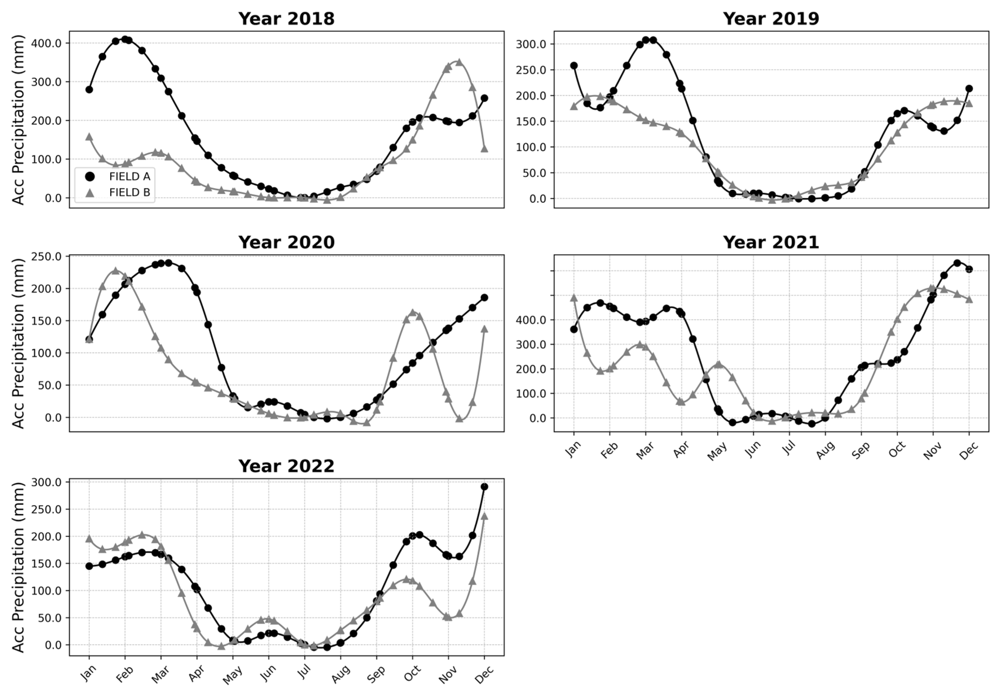
From September to December, an increase in VV and VH indices was observed. This increase may be related to the return of the rainy season, which raises soil moisture content. Indeed, during this same period, there is an increase in the monthly accumulated precipitation, elevating soil moisture levels. Additionally, the planting period for agricultural crops, which occurs between September and October, also influences this phenomenon, as increased biomass intensifies signal backscatter [57]. However, during the same period, the VV/VH index showed a decline. According to studies, the VV polarization band is particularly more sensitive to soil moisture compared to the VH band, leading to a reduction in the VV/VH index during this period [58,59].

Between December and January, a stabilization of VV and VH backscatter values is observed. This phenomenon occurs because, with the crop biomass fully developed, there is an attenuation effect from the canopy on the bands, reducing their sensitivity to soil moisture variation. Ref. [59] showed that the sensitivity of VV and VH bands to soil moisture variation decreases with the increase in vegetation cover growth (NDVI) and is stronger in the VV polarization than in the cross-polarization VH. El Hajj et al. [57] demonstrated that the VV polarization C-band penetrates the maize canopy even when the crop is at its biomass peak (NDVI > 0.7). However, penetration was limited in wheat and pastures. Therefore, during the crop canopy development, vegetation may become the primary component contributing to the volume scattering of the backscattered signal, while the influence of soil may become secondary. Finally, between April and August, there is a strong downward trend in backscatter values for both VV and VH polarizations. This behavior may be associated with the decrease in precipitation during this period, resulting in lower soil moisture content. Since the decrease in backscatter is more pronounced in VV polarization compared to VH, an increase in the VV/VH ratio is observed.

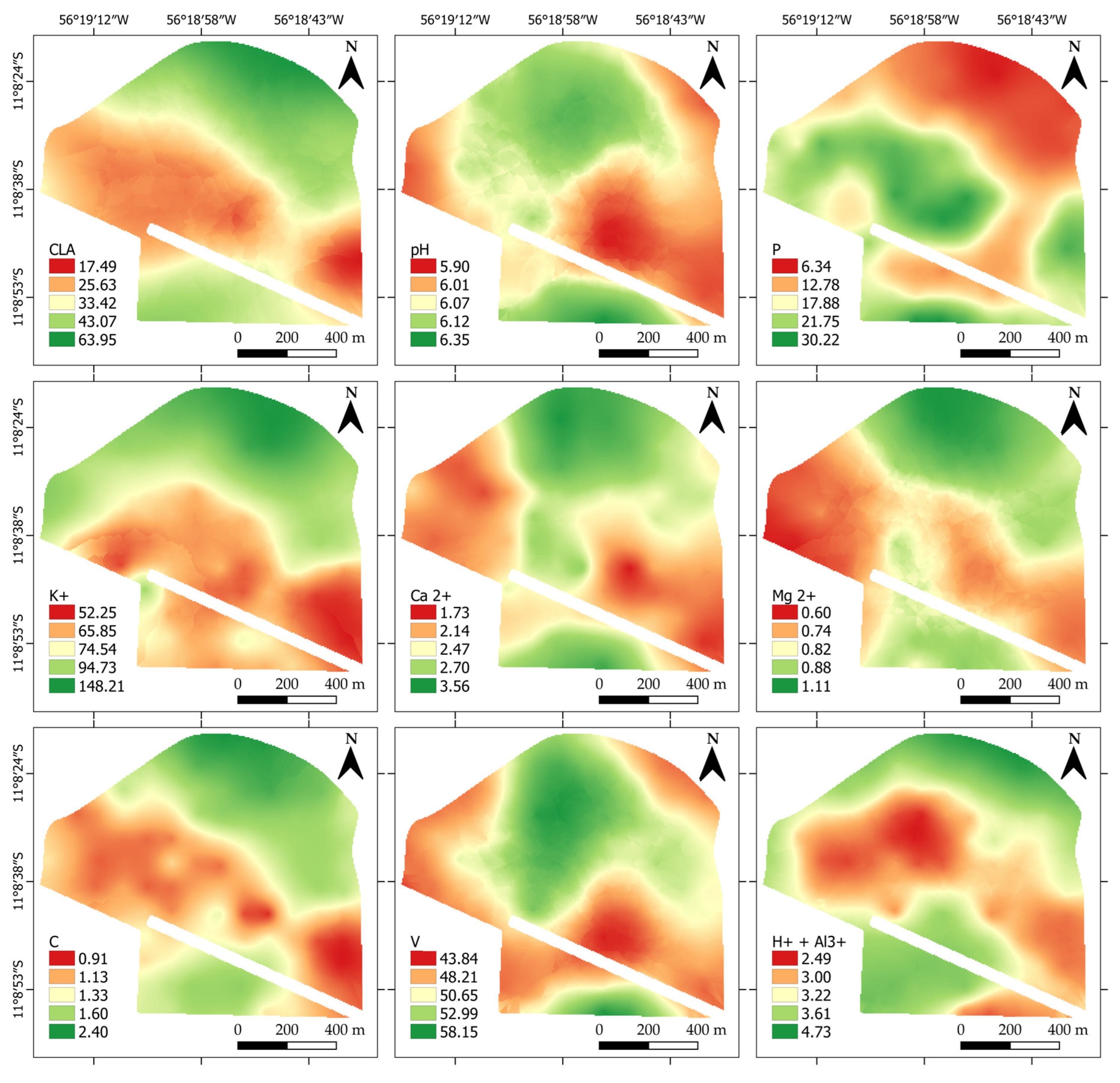
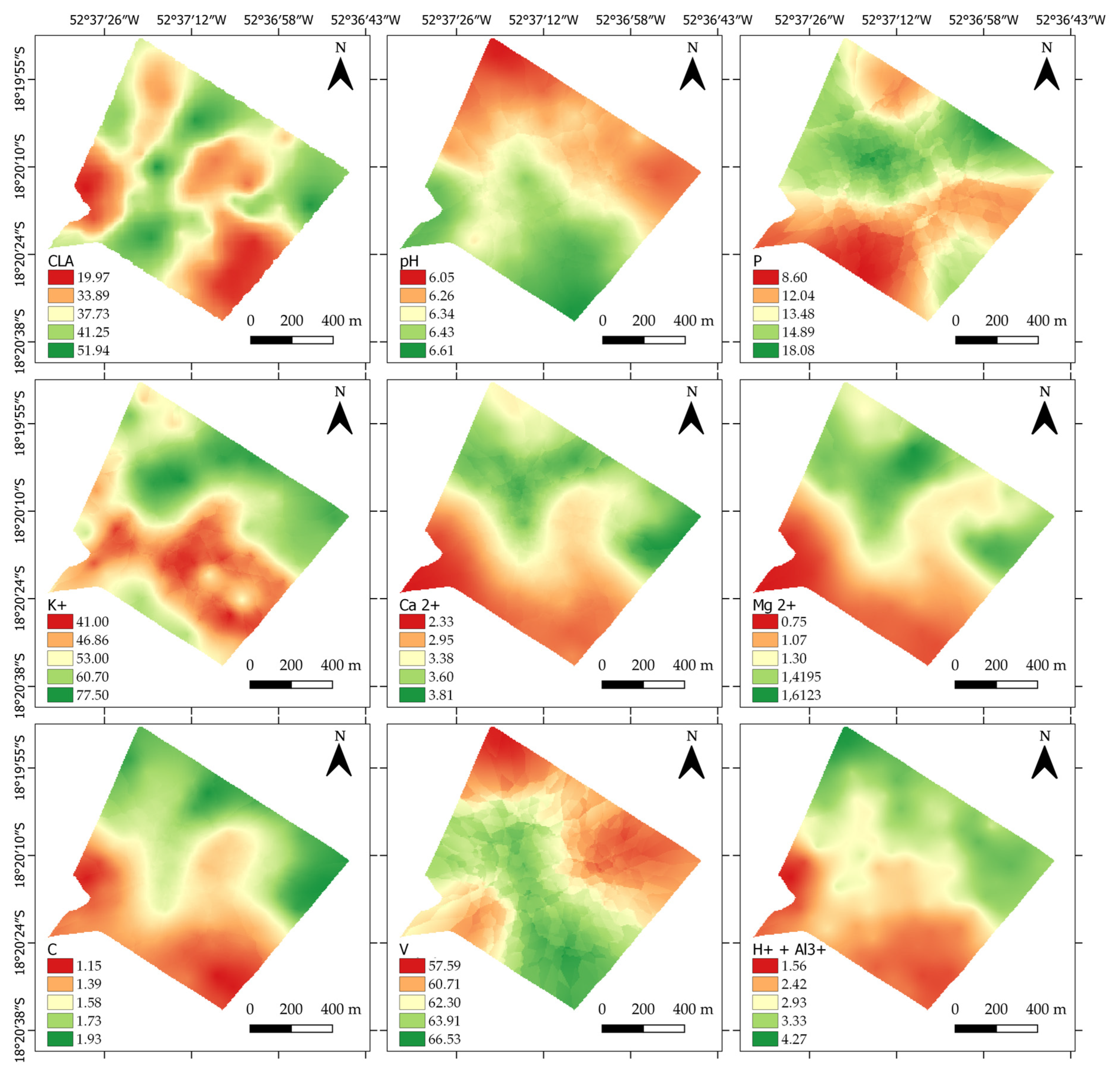
The evaluation of experimental semivariograms in GRID-1, for both fields, highlighted the spatial dependence of soil attributes. The SDI, which relates the nugget effect to the sill to quantify the spatial dependence of these attributes, was found to be less than 75% for most attributes. This indicates strong spatial dependence (less than 25%) and moderate spatial dependence (between 25% and 75%), as suggested by [52]. In this context, kriging emerges as an excellent method for the interpolation and estimation of soil attributes in unsampled locations.

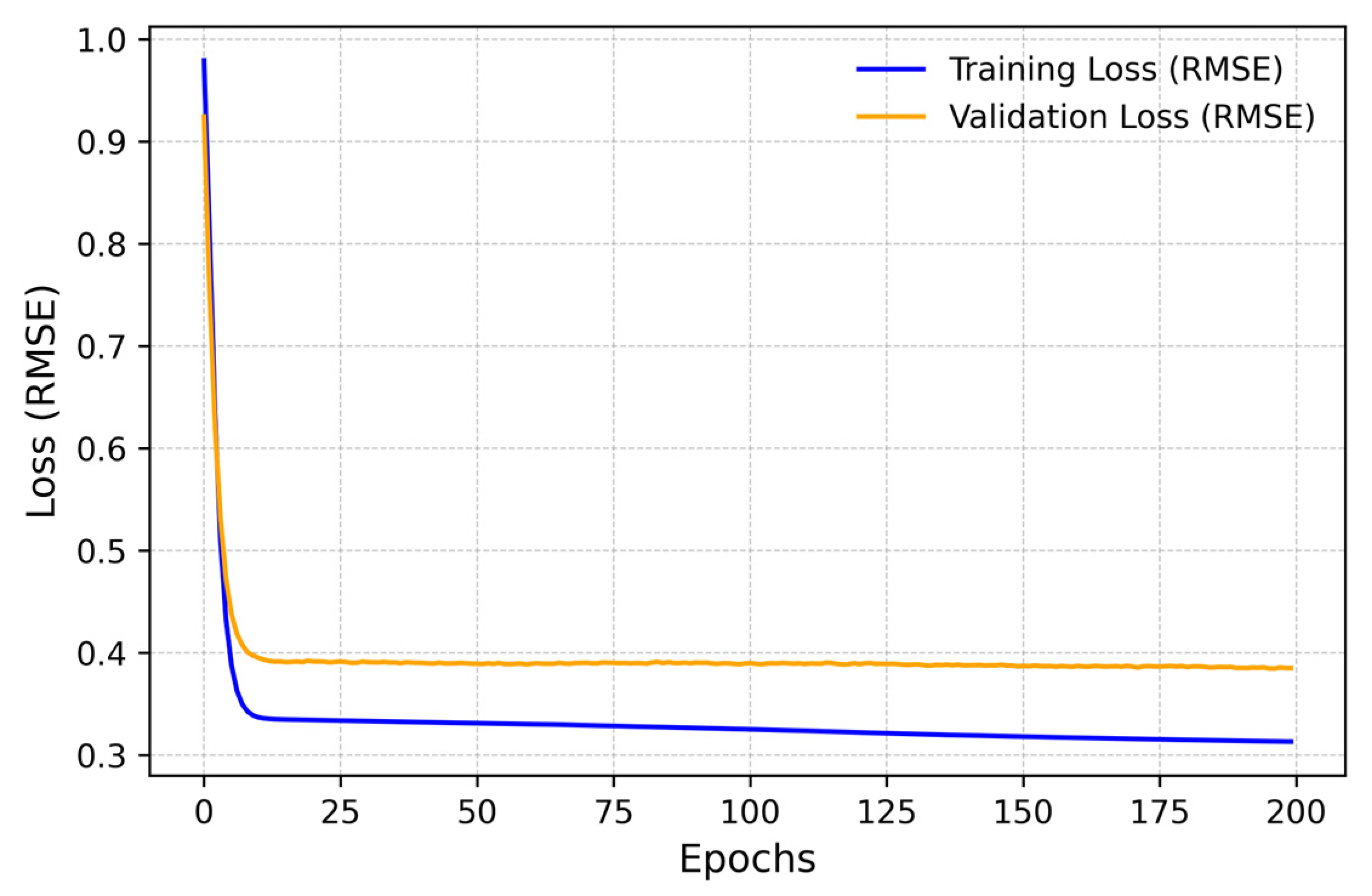
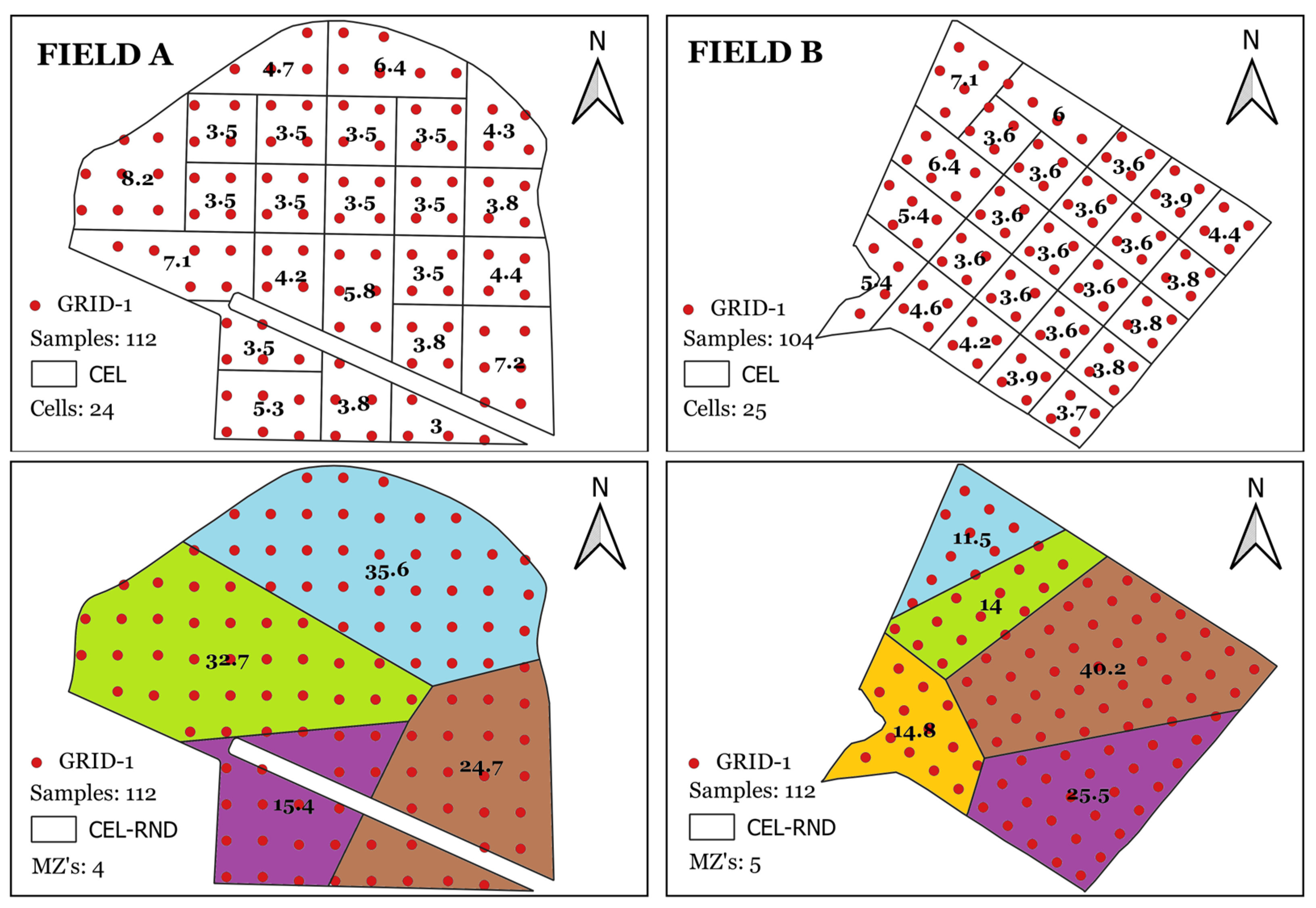
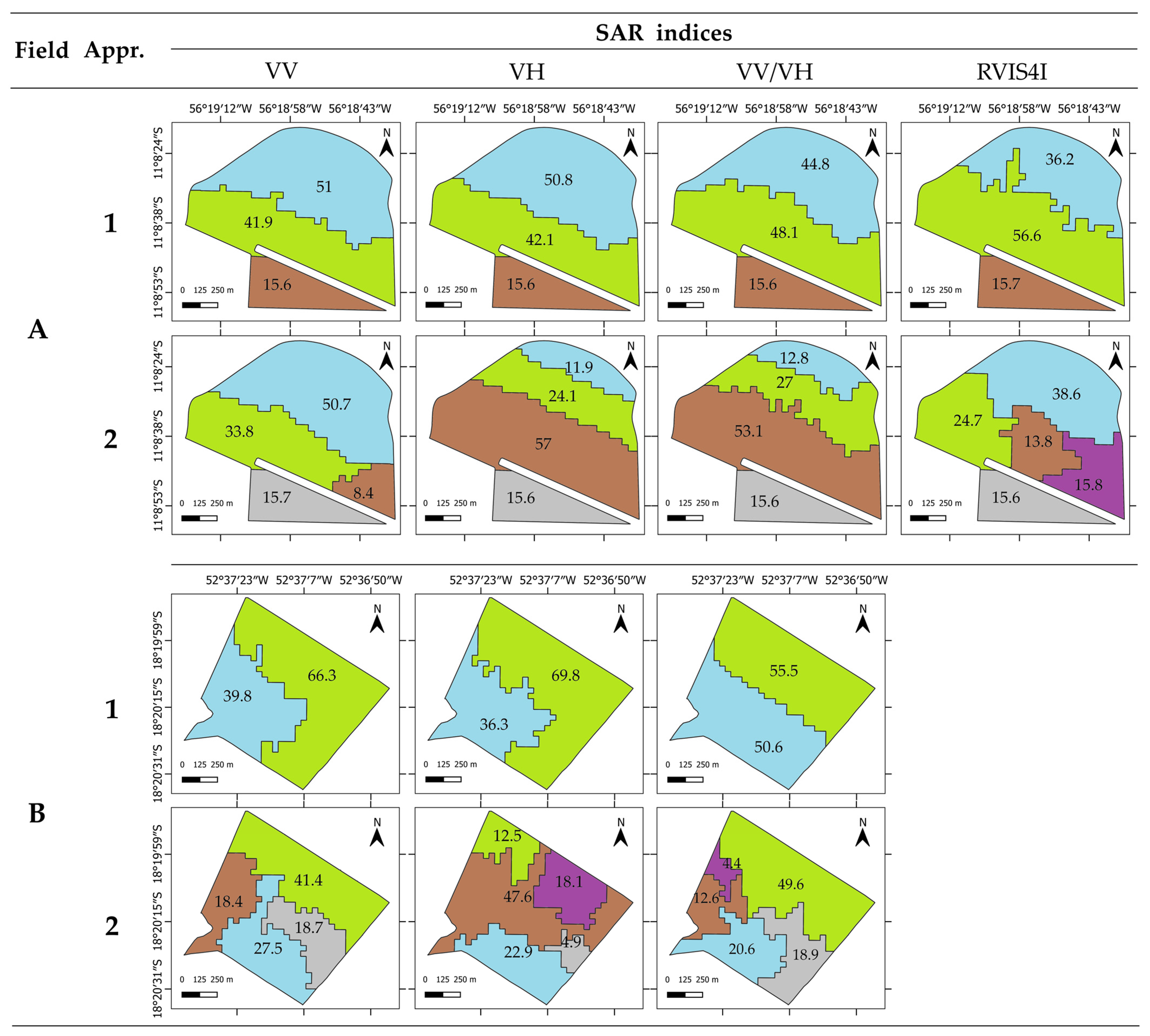
The VV and VH backscatter bands, along with the VV/VH and RVI4SI indices, showed variations in the size, shape, and number of MZs when subjected to Approaches 1 and 2. Approach 2, which applies clustering on features extracted from SAR time series via autoencoders, tended to generate more MZs in both fields compared to Approach 1, which performs clustering directly on the time series. Autoencoders belong to a specific class of deep artificial neural networks. They are designed to compress an input into a more compact representation and then reverse that compression, aiming for the reconstructed input to resemble the original as closely as possible [60]. The features extracted by the autoencoder, represented by the compact part, can capture nuances and patterns in the data that the raw representation cannot. This leads to a more detailed segmentation of the fields, resulting in a higher number of MZs. Another point to consider is that SAR images are characterized by high levels of noise [61]. Therefore, the use of features extracted by autoencoders represents a less noisy version of the original data, as the learning process of the architecture extracts patterns that explain the temporal behavior of the backscatter. This factor may result in more accurate clustering and an increase in the number of MZs.

The VV/VH index, combined with Approach 2 based on autoencoders, tended to exhibit lower RMSE values for soil attribute estimation using the LOOCV strategy. Thus, it was able to produce MZs with greater precision compared to other SAR indices. The integration of VV and VH backscatter band information has shown superior performance compared to the isolated use of each band in various applications [62,63]. This phenomenon is justified by the fact that the VV/VH ratio minimizes acquisition system errors and provides more consistent indications over time than the isolated VH or VV backscatter, as pointed out by [34]. Additionally, certain studies indicate that the VV/VH index correlates more closely with the NDVI in the specific phenological stages of the crop. This suggests that this index helps in understanding not only the spatial variability of soil moisture but also the canopy structure and crop biomass—crucial aspects for defining MZs [64].

When analyzing the MZs derived from the VV/VH index using autoencoders in both fields, a statistical distinction was observed in at least one mean of each soil attribute originating from the MZs, except for V. Despite the high variability of Clay in the region, statistical differences were also detected in temporally unstable attributes, such as Ca²⁺, Mg²⁺, K⁺, etc. The ability of plants to access these attributes is strongly influenced by the soil’s ability to retain water in its macro- and micropores. Thus, the sensitivity of SAR data to soil moisture, as evidenced in several studies, is crucial in identifying the variability of these macro- and micronutrients present in the soil [25,59,65].

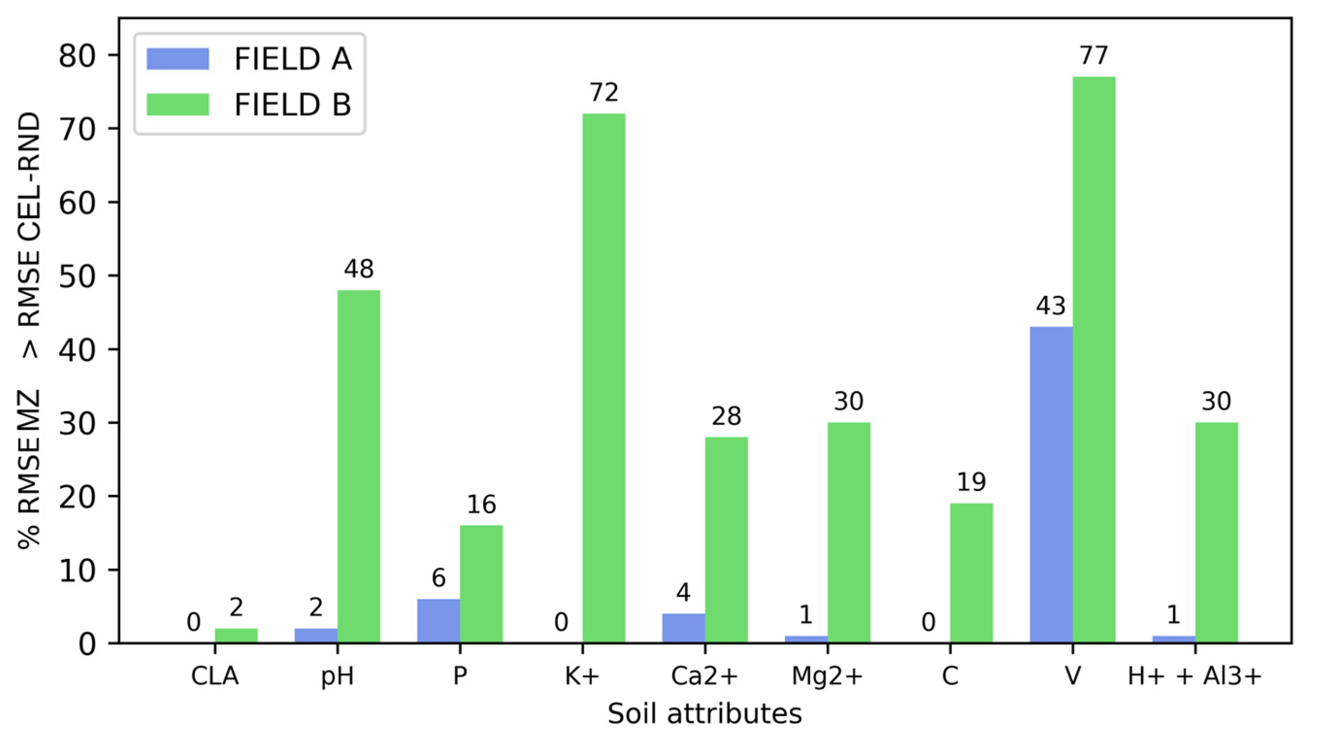
When analyzing the MZs generated by the VV/VH index using autoencoders in comparison to the randomly created cells (CEL-RND), the potential of the SAR index to delineate MZs was highlighted. Only for the soil attributes K⁺ and V in Field A was it observed that in more than 50% of the scenarios, the RMSE of the CEL-RND was lower than the RMSE estimated by the MZs. The best performance scenario of the VV/VH index against CEL-RND was observed for Clay in both fields. The Clay fraction of the soil is intrinsically linked to water retention [66]. Therefore, the sensitivity of SAR data to soil moisture may be one of the explanations for the high correlation observed between the MZs and Clay variability in the fields. Clay content exhibits a relatively stable spatial distribution over time, which can provide greater robustness and consistency in the delineation of MZs using the proposed method, especially considering that these zones are expected to have a predominantly static character. However, this study employed a five-year time series, and further research is needed to investigate the minimum time interval required to construct a temporal series that leads to consistent MZ delineations over time.

When evaluating the various sampling methods, it was observed that the method based on GRID-1 stood out, recording the lowest errors (lower RMSE) for all soil attributes. This result is justified by the fact that the fields investigated in this study exhibited high and moderate spatial dependencies for soil attributes, as indicated by the SDI. In such contexts, the fitting of semivariograms combined with kriging interpolation, the approach adopted in our study, tends to provide good estimates. In contrast, the significant spatial variability suggests that the CONV method, which attempts to represent the field through a single soil sample, may not be efficient. This observation is reinforced by noting that in the fields analyzed in this study, the CONV method had the highest RMSE values, indicating lower accuracy in the estimates of soil attributes.

The MZs delineated from the SAR data showed superiority compared to the CONV, CEL, and CEL-RND methods, being occasionally surpassed only by the CEL and CEL-RND methods. Therefore, in scenarios with limited financial resources where conventional sampling is chosen, SAR data can be used to guide sampling through MZs. This methodology, presented in this study, offers specialists the opportunity to provide services remotely, eliminating the need for field trips. This results in cost savings and facilitates the implementation of precision agriculture, even for small farmers. However, future research should be conducted to investigate the impact of reducing the time series in areas without overlapping satellite passes, where temporal resolution consequently decreases. Additionally, as evidenced, there is significant variation in backscatter intensity throughout the year, primarily influenced by fluctuations in precipitation. Thus, it is also suggested that future studies assess the possibility of using images acquired during specific periods of the year. Additionally, both areas analyzed in this study are located in the Brazilian Cerrado, a region characterized by a tropical climate and relatively flat terrain. Therefore, it is recommended that future studies be conducted in other parts of the country, especially in southern Brazil, which includes temperate climate zones and distinct topographic features such as high altitudinal variation and steep slopes. Expanding the validation in this way would allow for a broader assessment of the applicability and scalability of the proposed methodology across diverse geographic contexts.

5. Conclusions

The strategy combining autoencoders with the VV/VH index resulted in more accurate estimates of soil attributes compared to other Synthetic Aperture Radar (SAR) indices. The GRID-1 method, which uses a high-density point grid followed by kriging interpolation, stood out as the most effective technique for mapping soil attributes, while the conventional soil sampling method (CONV) performed the least satisfactorily. The Management Zones (MZs) delineated using the VV/VH index based on autoencoders outperformed the CONV method, the random cell-based soil sampling method (CEL-RND), and, in many cases, the rectangular cell-based soil sampling method (CEL). These findings are encouraging and indicate the potential of SAR data in analyzing soil variability and defining MZs.

This method has the potential to be integrated into digital platforms that use, for example, Google Earth Engine to provide Sentinel-1 data at the scale of agricultural fields. MZs generated using autoencoders applied to the VV/VH index can serve as an intelligent guide for soil sampling, directing sampling points in a more efficient and representative way. In addition to providing the sampling points, the shapefile with the Management Zones can be made available to guide agricultural machinery operations in defining crop treatment levels, such as cultivars, planting density, and fertilizers. Given that training the autoencoder is computationally intensive, this step would normally be performed offline by technical teams, but once trained, the model can be deployed as a lightweight module for automated MZ delineation on cloud platforms. This facilitates accessibility and scalability, even for small farmers.

References

1. de Queiroz, D.M.; de Coelho, A.L.F.; Valente, D.S.M.; Schueller, J.K. Sensors Applied to Digital Agriculture: A Review. Rev. Ciência Agronômica 2020, 51, e20207751. [Google Scholar] [CrossRef]
2. Franzen, D.W.; Peck, T.R. Field Soil Sampling Density for Variable Rate Fertilization. J. Prod. Agric. 1995, 8, 568–574. [Google Scholar] [CrossRef]
3. Lauzon, J.D.; O’Halloran, I.P.; Fallow, D.J.; von Bertoldi, A.P.; Aspinall, D. Spatial Variability of Soil Test Phosphorus, Potassium, and PH of Ontario Soils. Agron. J. 2005, 97, 524–532. [Google Scholar] [CrossRef]
4. Lawrence, P.G.; Roper, W.; Morris, T.F.; Guillard, K. Guiding Soil Sampling Strategies Using Classical and Spatial Statistics: A Review. Agron. J. 2020, 112, 493–510. [Google Scholar] [CrossRef]
5. Webster, R.; Oliver, M.A. Sample Adequately to Estimate Variograms of Soil Properties. J. Soil Sci. 1992, 43, 177–192. [Google Scholar] [CrossRef]
6. Fleming, K.L.; Westfall, D.G.; Wiens, D.W.; Brodahl, M.C. Evaluating Farmer Defined Management Zone Maps for Variable Rate Fertilizer Application. Precis. Agric. 2000, 2, 201–215. [Google Scholar] [CrossRef]
7. Bottega, E.L.; Safanelli, J.L.; Zeraatpisheh, M.; Amado, T.J.C.; de Queiroz, D.M.; Oliveira, Z.B. de Site-Specific Management Zones Delineation Based on Apparent Soil Electrical Conductivity in Two Contrasting Fields of Southern Brazil. Agronomy 2022, 12, 1390. [Google Scholar] [CrossRef]
8. Brock, A.; Brouder, S.M.; Blumhoff, G.; Hofmann, B.S. Defining Yield-Based Management Zones for Corn-Soybean Rotations. Agron. J. 2005, 97, 1115–1128. [Google Scholar] [CrossRef]
9. Damian, J.M.; de Pias, O.H.C.; Cherubin, M.R.; da Fonseca, A.Z.; Fornari, E.Z.; Santi, A.L. Applying the NDVI from Satellite Images in Delimiting Management Zones for Annual Crops. Sci. Agric. 2020, 77, e20180055. [Google Scholar] [CrossRef]
10. Jaynes, D.B.; Colvin, T.S.; Kaspar, T.C. Identifying Potential Soybean Management Zones from Multi-Year Yield Data. Comput. Electron. Agric. 2005, 46, 309–327. [Google Scholar] [CrossRef]
11. Peralta, N.R.; Costa, J.L. Delineation of Management Zones with Soil Apparent Electrical Conductivity to Improve Nutrient Management. Comput. Electron. Agric. 2013, 99, 218–226. [Google Scholar] [CrossRef]
12. Valente, D.S.M.; de Queiroz, D.M.; Pinto, F.d.A.d.C.; Santos, N.T.; Santos, F.L. Definition of Management Zones in Coffee Production Fields Based on Apparent Soil Electrical Conductivity. Sci. Agric. 2012, 69, 173–179. [Google Scholar] [CrossRef]
13. Moral, F.J.; Terrón, J.M.; Silva, J.R.M. da Delineation of Management Zones Using Mobile Measurements of Soil Apparent Electrical Conductivity and Multivariate Geostatistical Techniques. Soil Tillage Res. 2010, 106, 335–343. [Google Scholar] [CrossRef]
14. Saey, T.; Van Meirvenne, M.; Vermeersch, H.; Ameloot, N.; Cockx, L. A Pedotransfer Function to Evaluate the Soil Profile Textural Heterogeneity Using Proximally Sensed Apparent Electrical Conductivity. Geoderma 2009, 150, 389–395. [Google Scholar] [CrossRef]
15. McFadden, J.; Njuki, E.; Griffin, T. Precision Agriculture in the Digital Era: Recent. Adoption on U.S. Farms; AgEcon Search Waite Library: St. Paul, MN, USA, 2023. [Google Scholar]
16. Ju, J.; Roy, D.P. The Availability of Cloud-Free Landsat ETM+ Data over the Conterminous United States and Globally. Remote Sens. Environ. 2008, 112, 1196–1211. [Google Scholar] [CrossRef]
17. Wei, J.; Huang, W.; Li, Z.; Sun, L.; Zhu, X.; Yuan, Q.; Liu, L.; Cribb, M. Cloud Detection for Landsat Imagery by Combining the Random Forest and Superpixels Extracted via Energy-Driven Sampling Segmentation Approaches. Remote Sens. Environ. 2020, 248, 112005. [Google Scholar] [CrossRef]
18. Torres, R.; Snoeij, P.; Geudtner, D.; Bibby, D.; Davidson, M.; Attema, E.; Potin, P.; Rommen, B.; Floury, N.; Brown, M.; et al. GMES Sentinel-1 Mission. Remote Sens. Environ. 2012, 120, 9–24. [Google Scholar] [CrossRef]
19. Bioresita, F.; Puissant, A.; Stumpf, A.; Malet, J.-P. Fusion of Sentinel-1 and Sentinel-2 Image Time Series for Permanent and Temporary Surface Water Mapping. Int. J. Remote Sens. 2019, 40, 9026–9049. [Google Scholar] [CrossRef]
20. Miles, K.E.; Willis, I.C.; Benedek, C.L.; Williamson, A.G.; Tedesco, M. Toward Monitoring Surface and Subsurface Lakes on the Greenland Ice Sheet Using Sentinel-1 SAR and Landsat-8 OLI Imagery. Front Earth Sci. 2017, 5, 251152. [Google Scholar] [CrossRef]
21. Vickers, H.; Malnes, E.; Høgda, K.-A. Long-Term Water Surface Area Monitoring and Derived Water Level Using Synthetic Aperture Radar (SAR) at Altevatn, a Medium-Sized Arctic Lake. Remote Sens. 2019, 11, 2780. [Google Scholar] [CrossRef]
22. Xing, L.; Tang, X.; Wang, H.; Fan, W.; Wang, G. Monitoring Monthly Surface Water Dynamics of Dongting Lake Using Sentinal-1 Data at 10 m. PeerJ 2018, 6, e4992. [Google Scholar] [CrossRef] [PubMed]
23. Gorrab, A.; Zribi, M.; Baghdadi, N.; Mougenot, B.; Fanise, P.; Chabaane, Z. Retrieval of Both Soil Moisture and Texture Using TerraSAR-X Images. Remote Sens. 2015, 7, 10098–10116. [Google Scholar] [CrossRef]
24. Lee, J.H.; Kim, H.-C. The Impact of Sentinel-1-Corrected Fractal Roughness on Soil Moisture Retrievals. Fractal Fract. 2024, 8, 137. [Google Scholar] [CrossRef]
25. Balenzano, A.; Mattia, F.; Satalino, G.; Lovergine, F.P.; Palmisano, D.; Peng, J.; Marzahn, P.; Wegmüller, U.; Cartus, O.; Dąbrowska-Zielińska, K.; et al. Sentinel-1 Soil Moisture at 1 Km Resolution: A Validation Study. Remote Sens. Environ. 2021, 263, 112554. [Google Scholar] [CrossRef]
26. Chaudhary, S.K.; Srivastava, P.K.; Gupta, D.K.; Kumar, P.; Prasad, R.; Pandey, D.K.; Das, A.K.; Gupta, M. Machine Learning Algorithms for Soil Moisture Estimation Using Sentinel-1: Model Development and Implementation. Adv. Space Res. 2022, 69, 1799–1812. [Google Scholar] [CrossRef]
27. Rossini, P.R.; Ciampitti, I.A.; Hefley, T.; Patrignani, A. A Soil Moisture-based Framework for Guiding the Number and Location of Soil Moisture Sensors in Agricultural Fields. Vadose Zone J. 2021, 20, e20159. [Google Scholar] [CrossRef]
28. Azizi, K.; Garosi, Y.; Ayoubi, S.; Tajik, S. Integration of Sentinel-1/2 and Topographic Attributes to Predict the Spatial Distribution of Soil Texture Fractions in Some Agricultural Soils of Western Iran. Soil Tillage Res. 2023, 229, 105681. [Google Scholar] [CrossRef]
29. Garosi, Y.; Ayoubi, S.; Nussbaum, M.; Sheklabadi, M.; Nael, M.; Kimiaee, I. Use of the Time Series and Multi-Temporal Features of Sentinel-1/2 Satellite Imagery to Predict Soil Inorganic and Organic Carbon in a Low-Relief Area with a Semi-Arid Environment. Int. J. Remote Sens. 2022, 43, 6856–6880. [Google Scholar] [CrossRef]
30. Mirzaeitalarposhti, R.; Shafizadeh-Moghadam, H.; Taghizadeh-Mehrjardi, R.; Demyan, M.S. Digital Soil Texture Mapping and Spatial Transferability of Machine Learning Models Using Sentinel-1, Sentinel-2, and Terrain-Derived Covariates. Remote Sens. 2022, 14, 5909. [Google Scholar] [CrossRef]
31. Yang, R.-M.; Guo, W.-W. Modelling of Soil Organic Carbon and Bulk Density in Invaded Coastal Wetlands Using Sentinel-1 Imagery. Int. J. Appl. Earth Obs. Geoinf. 2019, 82, 101906. [Google Scholar] [CrossRef]
32. Frison, P.-L.; Fruneau, B.; Kmiha, S.; Soudani, K.; Dufrêne, E.; Le Toan, T.; Koleck, T.; Villard, L.; Mougin, E.; Rudant, J.-P. Potential of Sentinel-1 Data for Monitoring Temperate Mixed Forest Phenology. Remote Sens. 2018, 10, 2049. [Google Scholar] [CrossRef]
33. Kaushik, S.K.; Mishra, V.N.; Punia, M.; Diwate, P.; Sivasankar, T.; Soni, A.K. Crop Health Assessment Using Sentinel-1 SAR Time Series Data in a Part of Central India. Remote Sens. Earth Syst. Sci. 2021, 4, 217–234. [Google Scholar] [CrossRef]
34. Veloso, A.; Mermoz, S.; Bouvet, A.; Le Toan, T.; Planells, M.; Dejoux, J.-F.; Ceschia, E. Understanding the Temporal Behavior of Crops Using Sentinel-1 and Sentinel-2-like Data for Agricultural Applications. Remote Sens. Environ. 2017, 199, 415–426. [Google Scholar] [CrossRef]
35. Centro Nacional de Pesquisa de Solos. Solos Embrapa Sistema Brasileiro de Classificação de Solos; Centro Nacional de Pesquisa de Solos: Rio de Janeiro, Brazil, 2013; Volume 3. [Google Scholar]
36. Ferreira, M.M.; Fernandes, B.; Curi, N. Mineralogia Da Fração Argila e Estrutura de Latossolos Da Região Sudeste Do Brasil. Rev. Bras. Cienc. Solo 1999, 23, 507–514. [Google Scholar] [CrossRef]
37. Stasolla, M.; Neyt, X. An Operational Tool for the Automatic Detection and Removal of Border Noise in Sentinel-1 GRD Products. Sensors 2018, 18, 3454. [Google Scholar] [CrossRef] [PubMed]
38. Quegan, S.; Yu, J.J. Filtering of Multichannel SAR Images. IEEE Trans. Geosci. Remote Sens. 2001, 39, 2373–2379. [Google Scholar] [CrossRef]
39. Lee, J.-S.; Grunes, M.R.; de Grandi, G. Polarimetric SAR Speckle Filtering and Its Implication for Classification. IEEE Trans. Geosci. Remote Sens. 1999, 37, 2363–2373. [Google Scholar] [CrossRef]
40. Farr, T.G.; Rosen, P.A.; Caro, E.; Crippen, R.; Duren, R.; Hensley, S.; Kobrick, M.; Paller, M.; Rodriguez, E.; Roth, L.; et al. The Shuttle Radar Topography Mission. Rev. Geophys. 2007, 45, RG2004. [Google Scholar] [CrossRef]
41. Gorelick, N.; Hancher, M.; Dixon, M.; Ilyushchenko, S.; Thau, D.; Moore, R. Google Earth Engine: Planetary-Scale Geospatial Analysis for Everyone. Remote Sens. Environ. 2017, 202, 18–27. [Google Scholar] [CrossRef]
42. Mullissa, A.; Vollrath, A.; Odongo-Braun, C.; Slagter, B.; Balling, J.; Gou, Y.; Gorelick, N.; Reiche, J. Sentinel-1 SAR Backscatter Analysis Ready Data Preparation in Google Earth Engine. Remote Sens. 2021, 13, 1954. [Google Scholar] [CrossRef]
43. Chang, J.G.; Shoshany, M.; Oh, Y. Polarimetric Radar Vegetation Index for Biomass Estimation in Desert Fringe Ecosystems. IEEE Trans. Geosci. Remote Sens. 2018, 56, 7102–7108. [Google Scholar] [CrossRef]
44. Trudel, M.; Charbonneau, F.; Leconte, R. Using RADARSAT-2 Polarimetric and ENVISAT-ASAR Du-al-Polarization Data for Estimating Soil Moisture over Agricultural Fields. Can. J. Remote Sens. 2012, 38, 514–527. [Google Scholar] [CrossRef]
45. Filgueiras, R.; Mantovani, E.C.; Althoff, D.; Fernandes Filho, E.I.; Cunha, F.F. da Crop NDVI Monitoring Based on Sentinel 1. Remote Sens. 2019, 11, 1441. [Google Scholar] [CrossRef]
46. Maldonado, W.; Valeriano, T.T.B.; de Souza Rolim, G. EVAPO: A Smartphone Application to Estimate Poten-tial Evapotranspiration Using Cloud Gridded Meteorological Data from NASA-POWER System. Comput. Electron. Agric. 2019, 156, 187–192. [Google Scholar] [CrossRef]
47. Bezdek, J.C.; Ehrlich, R.; Full, W. FCM: The Fuzzy c-Means Clustering Algorithm. Comput. Geosci. 1984, 10, 191–203. [Google Scholar] [CrossRef]
48. Hoang, D.-T.; Kang, H.-J. A Survey on Deep Learning Based Bearing Fault Diagnosis. Neurocomputing 2019, 335, 327–335. [Google Scholar] [CrossRef]
49. Schmidt-Hieber, J. Nonparametric Regression Using Deep Neural Networks with ReLU Activation Function. Ann. Stat. 2020, 48, 1875–1897. [Google Scholar] [CrossRef]
50. Voronoi, G. Nouvelles Applications Des Paramètres Continus à La Théorie Des Formes Quadratiques. Deu-xième Mémoire. Recherches Sur Les Parallélloèdres Primitifs. J. Reine Angew. Math. (Crelles J.) 1908, 1908, 198–287. [Google Scholar] [CrossRef]
51. Isaaks, E.H.; Srivastava, R.M. Applied Geostatistics; Oxford University Press: New York, NY, USA, 1989. [Google Scholar]
52. Cambardella, C.A.; Moorman, T.B.; Novak, J.M.; Parkin, T.B.; Karlen, D.L.; Turco, R.F.; Konopka, A.E. Field-Scale Variability of Soil Properties in Central Iowa Soils. Soil Sci. Soc. Am. J. 1994, 58, 1501–1511. [Google Scholar] [CrossRef]
53. Pereira, G.W.; Valente, D.S.M.; de Queiroz, D.M.; Coelho, A.L.d.F.; de Costa, M.M.; Grift, T. Smart-Map: An Open-Source QGIS Plugin for Digital Mapping Using Machine Learning Techniques and Ordinary Kriging. Agronomy 2022, 12, 1350. [Google Scholar] [CrossRef]
54. Ahl, D.E.; Gower, S.T.; Burrows, S.N.; Shabanov, N.V.; Myneni, R.B.; Knyazikhin, Y. Monitoring Spring Can-opy Phenology of a Deciduous Broadleaf Forest Using MODIS. Remote Sens. Environ. 2006, 104, 88–95. [Google Scholar] [CrossRef]
55. Moran, M.S.; Alonso, L.; Moreno, J.F.; Cendrero Mateo, M.P.; de la Cruz, D.F.; Montoro, A. A RADARSAT-2 Quad-Polarized Time Series for Monitoring Crop and Soil Conditions in Barrax, Spain. IEEE Trans. Geosci. Remote Sens. 2012, 50, 1057–1070. [Google Scholar] [CrossRef]
56. Pelta, R.; Beeri, O.; Tarshish, R.; Shilo, T. Sentinel-1 to NDVI for Agricultural Fields Using Hyperlocal Dy-namic Machine Learning Approach. Remote Sens. 2022, 14, 2600. [Google Scholar] [CrossRef]
57. El Hajj, M.; Baghdadi, N.; Bazzi, H.; Zribi, M. Penetration Analysis of SAR Signals in the C and L Bands for Wheat, Maize, and Grasslands. Remote Sens. 2018, 11, 31. [Google Scholar] [CrossRef]
58. Amazirh, A.; Merlin, O.; Er-Raki, S.; Gao, Q.; Rivalland, V.; Malbeteau, Y.; Khabba, S.; Escorihuela, M.J. Re-trieving Surface Soil Moisture at High Spatio-Temporal Resolution from a Synergy between Sentinel-1 Radar and Landsat Thermal Data: A Study Case over Bare Soil. Remote Sens. Environ. 2018, 211, 321–337. [Google Scholar] [CrossRef]
59. Bousbih, S.; Zribi, M.; Lili-Chabaane, Z.; Baghdadi, N.; El Hajj, M.; Gao, Q.; Mougenot, B. Potential of Senti-nel-1 Radar Data for the Assessment of Soil and Cereal Cover Parameters. Sensors 2017, 17, 2617. [Google Scholar] [CrossRef]
60. Bank, D.; Koenigstein, N.; Giryes, R. Autoencoders. In Machine Learning for Data Science Handbook; Springer International Publishing: Cham, Switzerland, 2023; pp. 353–374. [Google Scholar]
61. Schmidt, K.; Schwerdt, M.; Miranda, N.; Reimann, J. Radiometric Comparison within the Sentinel-1 SAR Constellation over a Wide Backscatter Range. Remote Sens. 2020, 12, 854. [Google Scholar] [CrossRef]
62. Bazzi, H.; Baghdadi, N.; El Hajj, M.; Zribi, M.; Minh, D.H.T.; Ndikumana, E.; Courault, D.; Belhouchette, H. Mapping Paddy Rice Using Sentinel-1 SAR Time Series in Camargue, France. Remote Sens. 2019, 11, 887. [Google Scholar] [CrossRef]
63. Lasko, K.; Vadrevu, K.P.; Tran, V.T.; Justice, C. Mapping Double and Single Crop Paddy Rice With Senti-nel-1A at Varying Spatial Scales and Polarizations in Hanoi, Vietnam. IEEE J. Sel. Top Appl. Earth Obs. Remote Sens. 2018, 11, 498–512. [Google Scholar] [CrossRef]
64. Soudani, K.; Delpierre, N.; Berveiller, D.; Hmimina, G.; Vincent, G.; Morfin, A.; Dufrêne, É. Potential of C-Band Synthetic Aperture Radar Sentinel-1 Time-Series for the Monitoring of Phenological Cycles in a De-ciduous Forest. Int. J. Appl. Earth Obs. Geoinf. 2021, 104, 102505. [Google Scholar] [CrossRef]
65. Dabrowska-Zielinska, K.; Musial, J.; Malinska, A.; Budzynska, M.; Gurdak, R.; Kiryla, W.; Bartold, M.; Grzybowski, P. Soil Moisture in the Biebrza Wetlands Retrieved from Sentinel-1 Imagery. Remote Sens. 2018, 10, 1979. [Google Scholar] [CrossRef]
66. Ismail, S.M.; Ozawa, K. Improvement of Crop Yield, Soil Moisture Distribution and Water Use Efficiency in Sandy Soils by Clay Application. Appl. Clay Sci. 2007, 37, 81–89. [Google Scholar] [CrossRef]
Figure 1. Location of the study fields (Field A and Field B) in Brazil with the respective sampling points.
Agriengineering 07 00150 g001
Figure 2. Loss curves during training and validation of the autoencoder, expressed as root mean square error (RMSE) over 200 epochs. A sharp decrease is observed in the initial epochs, followed by stabilization, indicating a good model fit without signs of overfitting.
Agriengineering 07 00150 g002
Figure 3. Sampling methods defined by cells (CEL) and random cells (CEL-RND) for the study areas (Field A and Field B). The number within each zone represents its area in hectares.
Agriengineering 07 00150 g003
Figure 4. Pearson correlation between VV (vertical–vertical polarization) and VH (vertical–horizontal polarization) backscatter values and SAR indices obtained in Fields A and B. VH: Vertical–horizonal polarization; VV: vertical–vertical polarization; PRVI: Polarimetric Radar Vegetation Index; RVI4SI: Sentinel-1 Radar Vegetation Index; RVI: Radar Vegetation Index; NRPB: Normalized Ratio Procedure Between Bands; VV/VH: VV VH ratio; VH/VV: VH VV ratio.
Agriengineering 07 00150 g004
Figure 5. Scatter plots with smoothed lines of backscatter coefficients and SAR indices for Fields A and B over the months, covering the period from 1 January 2018 to 31 December 2022. VV: Vertical–vertical polarization; VH: vertical–horizonal polarization; VV/VH: VV VH ratio; RVI4SI: Sentinel-1 Radar Vegetation Index.
Agriengineering 07 00150 g005
Figure 6. Scatter plots with smoothed trend lines of monthly accumulated precipitation for Fields A and B, using NASA POWER data, in annual subplots from January 2018 to December 2022.
Agriengineering 07 00150 g006
Figure 7. Figures of soil attributes interpolated by ordinary kriging for Field A using GRID-1. CLA: Clay (%); pH: Active Acidity in water; P: Phosphorus (mg dm−3); K+: Potassium (mg dm−3); Ca2+: Calcium (cmolc dm−3); Mg2+: Magnesium (cmolc dm−3); C: Soil Organic Carbon (cmolc dm−3); V: Basis Saturations (%); H+ + Al3+: potential acidity (cmolc dm−3).
Agriengineering 07 00150 g007
Figure 8. Figures of soil attributes interpolated by ordinary kriging for Field B using GRID-1. CLA: Clay (%); pH: Active Acidity in water; P: Phosphorus (mg dm−3); K+: Potassium (mg dm−3); Ca2+: Calcium (cmolc dm−3); Mg2+: Magnesium (cmolc dm−3); C: Soil Organic Carbon (cmolc dm−3); V: Basis Saturations (%); H+ + Al3+: potential acidity (cmolc dm−3).
Agriengineering 07 00150 g008
Figure 9. Management Zones derived from SAR indices for both fields (A and B), using two approaches (Appr 1 and Appr 2). (A) Field A results using four SAR indices (VV, VH, VV/VH, RVI4SI) under Appr 1 and Appr 2 (rows 1 and 2, respectively). (B) Field B results using three SAR indices (VV, VH, VV/VH) under Appr 1 and Appr 2 (rows 1 and 2, respectively). Approaches 1 and 2 refer to clustering applied directly to SAR time series and to their reduced representations obtained via autoencoders, respectively. The colors are used solely to distinguish the boundaries of the management zones. The number within each zone represents its area in hectares. VV: Vertical–vertical polarization; VH: vertical–horizonal polarization; VV/VH: VV VH ratio: RVI4SI: Sentinel-1 Radar Vegetation Index.
Agriengineering 07 00150 g009
Figure 10. The percentage value by which the RMSE of the Management Zone (MZ) soil sampling method, delineated by Approach 2 and the SAR VV/VH index, was greater than the RMSE generated by the 1000 random cell soil sampling method (CEL-RND) scenarios. CLA: Clay (%); pH: Active Acidity in water; P: Phosphorus (mg dm−3); K+: Potassium (mg dm−3); Ca2+: Calcium (cmolc dm−3); Mg2+: Magnesium (cmolc dm−3); C: Soil Organic Carbon (cmolc dm−3); V: Basis Saturations (%); H+ + Al3+: potential acidity (cmolc dm−3).
Agriengineering 07 00150 g010