Article

Drone-Assisted Plant Stress Detection Using Deep Learning: A Comparative Study of YOLOv8, RetinaNet, and Faster R-CNN

1
Computer System Engineering Department, Palestine Technical University–Kadoorie, Tulkarem P305, Palestine
2
Computer Science Department, Palestine Technical University–Kadoorie, Tulkarem P305, Palestine
3
Lab-i* (Laboratoire d’Informatique), Université de Reims Champagne-Ardenne, 51100 Reims, France
*
Author to whom correspondence should be addressed.
AgriEngineering 2025, 7(8), 257; https://doi.org/10.3390/agriengineering7080257
Submission received: 21 June 2025 / Revised: 24 July 2025 / Accepted: 7 August 2025 / Published: 11 August 2025
(This article belongs to the Topic Digital Agriculture, Smart Farming and Crop Monitoring)

Abstract

Drones have been widely used in precision agriculture to capture high-resolution images of crops, providing farmers with advanced insights into crop health, growth patterns, nutrient deficiencies, and pest infestations. Although several machine and deep learning models have been proposed for plant stress and disease detection, their performance regarding accuracy and computational time still requires improvement, particularly under limited data. Therefore, this paper aims to address these challenges by conducting a comparative analysis of three State-of-the-Art object detection deep learning models: YOLOv8, RetinaNet, and Faster R-CNN, and their variants to identify the model with the best performance. To evaluate the models, the research uses a real-world dataset from potato farms containing images of healthy and stressed plants, with stress resulting from biotic and abiotic factors. The models are evaluated under limited conditions with original data of size 360 images and expanded conditions with augmented data of size 1560 images. The results show that YOLOv8 variants outperform the other models by achieving larger mAP@50 values and lower inference times on both the original and augmented datasets. The YOLOv8 variants achieve mAP@50 ranging from 0.798 to 0.861 and inference times ranging from 11.8 ms to 134.3 ms, while RetinaNet variants achieve mAP@50 ranging from 0.587 to 0.628 and inference times ranging from 118.7 ms to 158.8 ms, and Faster R-CNN variants achieve mAP@50 ranging from 0.587 to 0.628 and inference times ranging from 265 ms to 288 ms. These findings highlight YOLOv8’s robustness, speed, and suitability for real-time aerial crop monitoring, particularly in data-constrained environments.

1. Introduction

Agriculture is vital to the global economy and satisfies one of the basic human needs, which is food. However, plant stress and diseases significantly reduce the quantity and quality of crop production, causing economic losses and societal harm [1]. Consequently, farmers always look for methods to improve their crop yield and quality. Precision agriculture applies technology to enhance farming practices and improve resource management leading to increasing yields, reducing costs, and improving crop quality [2]. Among the technologies used in precision agriculture are drones that are gaining popularity due to their low cost, time efficiency, and high-resolution aerial images [3,4,5,6]. For instance, drones equipped with sensors and cameras can be used to monitor crop health, detect pests and illnesses, and identify stressed areas [7]. This information enables farmers to make better decisions regarding fertilization, irrigation, and other activities.
Drones generate large volumes of data that are difficult to process and analyze without the appropriate tools and expertise [8,9]. These data enable precise monitoring of crop health, early detection of stress factors, and data-driven decision-making, ultimately improving yield, resource efficiency, and sustainability in agriculture. So, different data analytics tools have been employed to help farmers understand data and identify plant diseases. However, studies found that each plant disease requires a customized algorithm that can distinguish between healthy and stressed plants in aerial images [10]. As a result, different deep learning and machine learning models have been proposed to analyze drone images and identify patterns and anomalies [11,12,13,14,15,16,17,18].
Deep learning models can automatically extract features and detect stresses and diseases in complex situations, such as overlapping leaves, and often outperform machine learning models [10]. Nevertheless, the performance of deep learning models in terms of accuracy and computational time still requires improvement to enable faster analysis and reduce errors that negatively impact farmer decision-making processes. Also, studies show that performance depends on the amount of data and suggest the use of augmentation techniques to increase dataset size and diversity [9,19,20]. Additionally, performance is a function of the intrinsic characteristics of image analysis algorithms, so studies suggest adopting more accurate and faster versions of deep learning, such as You Only Look Once (YOLO), new generations, and Faster Region-based Convolutional Neural Network (R-CNN) [20,21].
This research addresses performance limitations by proposing a comparative study of deep learning models: YOLOv8 [20,21,22], Faster R-CNN [23,24], and Retina Network (RetinaNet) [20,22,24,25], and their variants, aiming to identify the best model that can efficiently analyze crop aerial images. These models are tested using a real-world dataset, which was collected from the Aberdeen Research and Extension Center at the University of Idaho [25]. The dataset originally contained 360 aerial images and was augmented to 15,000 images of potato crops with labeled regions indicating healthy and stressed plants. The models’ performance is evaluated and compared based on mean Average Precision (mAP@50), precision, recall, and inference time. The results indicate that YOLOv8 variants outperform the other models as the YOLO variants have the largest mAP@50 values and the lowest inference times on both the original and augmented datasets.
This paper makes key contributions to the fields of precision agriculture, particularly plant stress detection, as follows:
  • The paper offers a detailed comparative analysis of three State-of-the-Art deep learning models: YOLOv8, Faster R-CNN, and RetinaNet, and their variants for aerial images of potato crops. The research highlights the most promising method for balancing accuracy and computational cost through performance evaluation.
  • The paper demonstrates how data augmentation mitigates data scarcity by introducing a larger dataset supporting a better training process and reducing the time and effort needed for manual collection and labeling of data.
  • The research emphasizes the use of lightweight, fast, and accurate deep learning models in real-world agricultural settings, enabling more automated, cost-effective, and scalable crop health monitoring with drones.

2. Related Work

Plant stress significantly decreases crop quality and quantity, leading to dramatic economic losses for farmers and societies. Therefore, detecting plant stress as early and accurately as possible is essential to minimize the loss in production and to enhance the quality of crops. Historically, plant stress and disease diagnosis have depended on experts’ knowledge and visual inspection of visible symptoms, such as spotting, discoloration, or malformations of leaves, stems, fruits, or flowers [26,27]. Many infections can often be characterized by an identifiable pattern that aids in diagnosis. However, human-based practices are time-consuming, labor-intensive, and prone to subjectivity, which leads to inconsistent and inaccurate diagnoses [10,26].

2.1. Drones for Precision Agriculture

Precision agriculture technologies revolutionize plant stress and disease detection and diagnosis by linking crop health with technological advancements in imaging, sensing, and AI analytics [2,28]. In fact, precision agriculture supports continuous real-time monitoring of plant health and enables early-stage stress detection even prior to visually observable symptoms. Importantly, precision agriculture reduces the need for manual labor and the variability of performing visual inspections of plant disease, which enhances the sustainability of agricultural production practices [10,26].
A major enabler of precision agriculture is Unmanned Aerial Vehicles (UAVs) known as drones, which are used for remote sensing in crop production. Drones allow farmers to accurately and quickly monitor ecosystem conditions including plant health, water stress, and soil conditions for very large areas [9,29]. Consequently, drone technology enhances the detection of plant abnormalities early, the allocation of resources appropriately, and supports data-driven agricultural decision-making [7,21,28]. Thus, the use of drones for detecting plant stress and disease reduces the costs and time of monitoring, and allows capturing high-resolution aerial imagery for accurate assessment [10,20,29,30].
As drones can generate a large number of high-resolution aerial images of plants, these images require automated and accurate analysis so that farmers can obtain the necessary knowledge about their crops. Recently, several machine learning and deep learning models have been proposed to analyze drone images, but deep learning models have shown superior accuracy because they automate the feature extraction process [9,21,31]. On the other hand, machine learning models are prone to errors because of manual feature identification; they struggle to distinguish between plant diseases with similar visual symptoms, and they are limited in their ability to handle large volumes of training data [9,32]. Deep learning (DL), which is a class of Artificial Neural Networks (ANN), has been a promising technique for data analysis as it uses ANN with multiple layers (deep neural networks) to automatically learn patterns and representations from data [32,33].

2.2. Deep Learning Models in Agriculture

In agriculture, deep learning models provide advanced capabilities for analyzing complex datasets, especially those generated by agricultural drones, to improve crop productivity [7,19,20,28,29,34]. Several studies used deep learning for the detection of biotic and abiotic crop stresses, such as cold damage [35], water stress [36,37], and nutrient deficiencies [17,18,38,39,40]. A survey of deep learning methods that are employed for detecting plant disease from drone images can be found at [9]. The majority of these methods use varieties of Convolutional Neural Network (CNN) models for the classification of diseases using a dataset of images for healthy and diseased plant leaves [23,41,42,43,44,45,46,47]. To increase accuracy and time efficiency, studies explored other models such as the Faster R-CNN (e.g., [23,24]), YOLOv2, YOLOv3, YOLOv8 [22], and RetinaNet (e.g., [20,22,24,25]), and they show that these models outperform the CNN-based methods. Table 1 shows a summary of related models and their accuracy measured by different metrics. Some papers in the table used different models but the table shows the one with the highest accuracy.
Beyond disease detection, deep learning was applied to crop yield prediction using Recurrent Neural Networks (RNNs) and Long Short-Term Memory (LSTM) networks [48,49]. Also, deep learning was used for object detection as a CNN model was applied for fruit counting [35,50,51]. Another object detection application is weed detection and management because deep learning enables the automatic detection of weeds and distinguishing between weeds and crops [41].
The review of the related work shows that several deep learning models have been proposed for analyzing aerial images of plants with a focus on disease detection. However, these models require large labeled datasets and high computational resources. To address these challenges, studies suggested the use of data augmentation to improve model performance and reduce the chance of overfitting [9,19,20]. Also, most of the proposed deep learning models are based on CNNs, and studies suggest faster evolved models, such as the new generation of YOLO [22], and Faster R-CNN [20,21]. Therefore, this research explores deep learning State-of-the-Art models: YOLOv8, RetinaNet, and Faster R-CNN, and their variants for the classification of healthy or stressed potato plants accurately and efficiently. Also, the research applies data augmentation to existing data to increase the number of images in the training dataset, undergoing the whole process of manual data collection and labeling.

3. Methodology

This research aims to identify the most effective deep learning model for determining crop health using drone images. The methodology used in this research starts with data collection, data preprocessing, exploratory analysis, model selection, and evaluation.

3.1. Dataset

The dataset in this research consists of drone images obtained from the Aberdeen Research and Extension Center at the University of Idaho [25]. The dataset comprises original and augmented multispectral images of potato plants to reflect real-world conditions of plants [25]. The dataset contains a comprehensive collection of aerial images captured using a Parrot Sequoia multispectral camera mounted on a 3DR Solo drone. The images were collected by a drone at an altitude of 3 m above ground at a speed of 0.5 m/s. These altitudes and speeds enable the capture of high-resolution images of plants, and subsequently, enable the recognition of crop stress in the field at the individual plant level. For the RGB sensor, the ground resolution of the images is 0.08 cm, and the footprint is 3.6 X 2.7 m per image. This ultra-high resolution was chosen deliberately to capture fine-grained visual symptoms of both biotic and abiotic plant stress, such as minor leaf spots, edge discoloration, or early wilting, which are often imperceptible in standard-resolution aerial imagery.
A time-lapse mode with a time interval set to 1.21 s was used for capturing the images. This dataset serves as a valuable resource for training machine learning models in the field of precision agriculture, specifically for crop health assessment.

3.2. Data Preprocessing and Augmentation

Although flying at such a low altitude increases the risk of capturing noisy or variable images due to motion blur, light reflection, or wind-induced plant movement, the benefits in terms of image detail outweighed these risks for our target task. To mitigate these issues, we implemented a preprocessing pipeline that includes contrast normalization to reduce lighting variability, noise filtering to reduce background artifacts, and geometric transformations (e.g., flips and rotations). The images taken by the drone were preprocessed by first undistorting and aligning them. Then, patches of images with each image size of 750×750 pixels were extracted from different spatial locations for each RGB image by cropping and rotating at 45, 90, and 135 degrees. This step resulted in a dataset of 360 high-resolution RGB image patches containing several rows of healthy and stressed potato plants.
However, the dataset presents a clear limitation in terms of the number of available images, which may negatively affect the performance and generalization of deep learning models. To overcome this issue, we applied data augmentation techniques to create additional and synthetic training samples by applying transformations that simulate real-world variations. Each original image was augmented to produce 10 additional samples, resulting in a total of 1500 distinct training images. Therefore, several transformations were performed randomly on each original image. Specifically, the augmentation pipeline includes the following:
  • Pixel intensity adjustments to simulate lighting variations;
  • Contrast modification using sigmoid-based enhancement;
  • Brightness changes via gamma correction;
  • Controlled random noise addition to simulate sensor artifacts and environmental conditions;
  • Geometric transformations including horizontal/vertical flips and rotations (at 90°, 180°, and 270°) to improve spatial diversity.

3.3. Exploratory Data Analysis

In this section, we present an in-depth exploration of both the original and the augmented dataset. This analysis forms the basis for understanding the dataset’s features and characteristics. We used the bounding box annotation technique to label potato plants according to their health status. Each visible leaf was enclosed within a rectangular bounding box and labeled as either “Healthy” or “Stressed.” This method supports easy and accurate identification and robust classification of individual plant instances at scale. Thus, object detection models are capable of capturing the spatial and categorical information associated with plant health conditions. In order to achieve dependable training and evaluation of detection frameworks, the dataset annotations required consistency throughout the dataset.
To analyze the spatial feature distribution further, we categorized bounding boxes according to their distinct spatial scale in relation to the image. Small-scale bounding boxes signify features that take up less than 10% of the image, which corresponds to detailed, lower leaf structures. These are often critical in the early detection of plant stress. Medium-scale bounding boxes range from 10% to 30% of the image, capturing moderately sized regions that offer visually informative context. Large-scale bounding boxes representing more than 30% of the image area are those that usually stand for the dominant structures of the plant sample. Table 2 shows that most bounding boxes in both “Healthy” and “Stressed” classes fall under the small-scale category, highlighting the prevalence of finer visual details in the dataset.
Sample images from both classes were visualized to gain a qualitative understanding of the data, as shown in Figure 1. This step provided valuable insights into the visual characteristics of healthy and stressed potato plants, which are instrumental in training the deep learning model.

3.4. Model Selection

In this work, we performed a comparative analysis of three prominent deep learning-based object detection frameworks: YOLOv8, RetinaNet, and Faster R-CNN. We evaluate whether these models could classify potato plants as healthy or stressed based on aerial images of potato leaves captured by drones. Each model was tested with multiple architectural and backbone configurations to assess performance.

3.4.1. YOLOv8 Variants

YOLOv8 (You Only Look Once version 8) is an efficient one-stage object detection architecture that performs real-time on-device object detection tasks. In contrast to previous versions which were used in different applications (e.g., [25,52,53]), YOLOv8 has an anchor-less style and a more flexible, modular architecture that allows for classification, object detection, and segmentation [54]. For this study, we evaluated five variants of YOLOv8, differing in the depth and width of the model, including the following:
YOLO8n (nano): This architecture is designed for ultra-low power and high-speed deployment.
YOLO8s (small): This architecture offers slightly better accuracy with some sacrifice to speed and resource consumption.
YOLO8m (medium): This architecture offers improved accuracy at a moderate cost of computation.
YOLO8l (large): This architecture is more precise than the medium variant but requires more powerful hardware.
YOLO8x (extra-large): This architecture is the most powerful variant with deeper and wider layers that provide enhanced performance.

3.4.2. Variants of RetinaNet

RetinaNet is a single-stage object detector notable for introducing Focal Loss, which mitigates the issue of class imbalance in dense detection tasks [55]. It is more efficient than the two-stage counterparts because it performs dense prediction in an image without requiring regional proposals. During our experiments, we applied three RetinaNet backbone networks:
ResNet-50: This architecture has medium depth with residual connections.
ResNet-101: This architecture is even deeper and more powerful in terms of representation.
ResNeXt-101: This architecture offers an improved residual network that applies grouped convolutions for higher accuracy and lower computational demand.
These backbones were selected to investigate the effect of model depth on the performance of detecting stressed and healthy potato plants.

3.4.3. Variants of the Faster R-CNN Method

Faster R-CNN is a commonly used two-stage model for object detection. It performs region proposal with a Region Proposal Network (RPN) and then classifies the objects by applying bounding box regression [56]. Faster R-CNN is often more accurate than one-stage models, especially when detailed spatial analysis is required. However, it is also slower. Just like with RetinaNet, we tested three Faster R-CNN backbone networks: ResNet-50, ResNet-101, and ResNeXt-101. With these Faster R-CNN backbones, we focus on low-resolution networks with higher versatility to reveal the impact of model complexity on classifying drone images of leaves.

3.5. Evaluation Metrics

We evaluate the effectiveness of the proposed model using a set of assessment measures that includes Mean Average Precision (mAP), which is a commonly used metric in object detection tasks. This metric calculates the average precision for each class and then takes the mean mAP@50 and mAP@50–95, which are both crucial metrics used to evaluate the performance of object detection models. The mAP@50 measures the average accuracy at an Intersection over Union (IoU) threshold of 0.50. It evaluates how well items having a modest overlap with ground-truth bounding boxes are localized by the model. It is particularly useful when object size or location varies slightly. mAP@50–95 is an extended metric developed to evaluate performance across a range of IoU thresholds, going from 0.50 to 0.95. It provides a more thorough and comprehensive understanding of the model’s accuracy.
Practically, both metrics are valuable tools for evaluating and comparing object detection models, with mAP@50–95 offering a more extensive evaluation across various levels of object overlap. In our context, mAP provides a comprehensive measure of the model’s precision across both “healthy” and “stressed” classes. A higher mAP indicates better performance in localizing and classifying objects accurately.
The second metric used in this research is precision, which measures the accuracy of positive predictions made by the model. For our task, precision indicates how well the model identifies “healthy” and “stressed” crops without misclassification. Precision is calculated as
P r e c i s i o n = T P T P + F P
where TP denotes true positives instances which are correctly predicted as positive, and FP denotes false positives instances which are incorrectly predicted as positive. Precision provides insight into the accuracy of positive predictions made by a model. Higher precision values indicate a lower rate of false positives, signifying a more reliable positive prediction performance.
The third metric is Recall, also known as sensitivity or true positive rate, which measures the ability of the model to detect all positive instances. It is calculated as
R e c a l l = T P T P + F N
where FN denotes false negative instances. In our context, recall quantifies the model’s ability to detect all instances of “healthy” and “stressed” crops in the dataset. A higher recall value indicates a lower rate of false negatives, highlighting a more comprehensive coverage of positive instances by the model.
The fourth metric is Inference Time, which refers to the time a trained model consumes to generate predictions or outputs for a given input during deployment. The inference time provides a quantitative measure of the computational efficiency of a model during deployment. It is crucial in real-time applications and scenarios where prompt predictions are required. Lower inference times are desirable as they indicate faster model response and reduced latency.

3.6. Experiment Setup

The selected model variants with different backbones were experimented on an NVIDIA GeForce RTX 3050 Laptop GPU with 4096 MiB of VRAM. The dataset was divided into a training set and a testing set. Table 3 shows a comprehensive overview of the distribution of annotated objects in the training and testing sets of the original and augmented data. We used data augmentation only on the training set; the testing set was left unaltered to ensure evaluation on real data and avoid misleading or biased results.
To ensure a fair and reproducible comparison, consistent training configurations were applied to the selected models. All models were trained on the dataset with a fixed input image size of 750 × 750 pixels. The YOLOv8 is trained for 300 epochs using the official Ultralytics implementation. The optimizer used was AdamW with an initial learning rate of 0.001. A batch size of 16 was used, and validation loss monitoring was applied for early stopping and checkpoint saving. The RetinaNet is trained for 50 epochs using the Stochastic Gradient Descent (SGD) optimizer with momentum = 0.9 and weight decay = 0.0005. The initial learning rate was 0.001, reduced by a factor of 0.1 every 10 epochs. A batch size of 8 was used. Finally, the Faster R-CNN is also trained for 50 epochs with the same optimizer and learning rate schedule as RetinaNet. It used Cross-Entropy Loss for classification and Smooth L1 Loss for localization. A batch size of 8 was maintained for consistency.

4. Results and Discussion

This section presents and discusses the results of evaluating YOLOv8m, RetinaNet, and Faster R-CNN on the original dataset and the augmented data focusing on two distinct classes: healthy and stressed. The choice of the original dataset was motivated by the need to establish a baseline performance under standard conditions before exploring augmented datasets. The original dataset serves as a vital reference point against which we can evaluate the effectiveness of data augmentation techniques which assist in understanding the model’s adaptability and effectiveness.

4.1. Results of Detection by YOLOv8

For all YOLOv8 variants, we trained the models using the default hyperparameters, as specified in the documentation [54]. Each model was trained for a total of 300 epochs with validation loss monitoring. Throughout the training process, we monitored key performance metrics, including loss curves, mAP, and class-specific precision-recall curves. The patience-based early stopping mechanism was employed to prevent overfitting and select the best-performing model. If no significant improvement in validation loss was observed for 100 consecutive epochs, training was paused, and the model with the lowest validation loss was then selected. The performance of YOLOv8 variants on the original and augmented datasets is shown in Table 4.
As shown in Table 4, YOLOv8x achieved the highest values of precision, recall, mAP@50, and mAP@50–95 on the augmented dataset. This indicates that YOLOv8x has superior accuracy and generalization. The smallest model, YOLOv8n (nano), also has noticeable gains with augmentation as mAP@50–95 increases from 0.619 to 0.719, which highlights the value of augmentation even for lightweight models. It is clear that larger models consistently outperform smaller ones, and the data augmentation consistently enhances the detection of “healthy” and “stressed” potato plants.
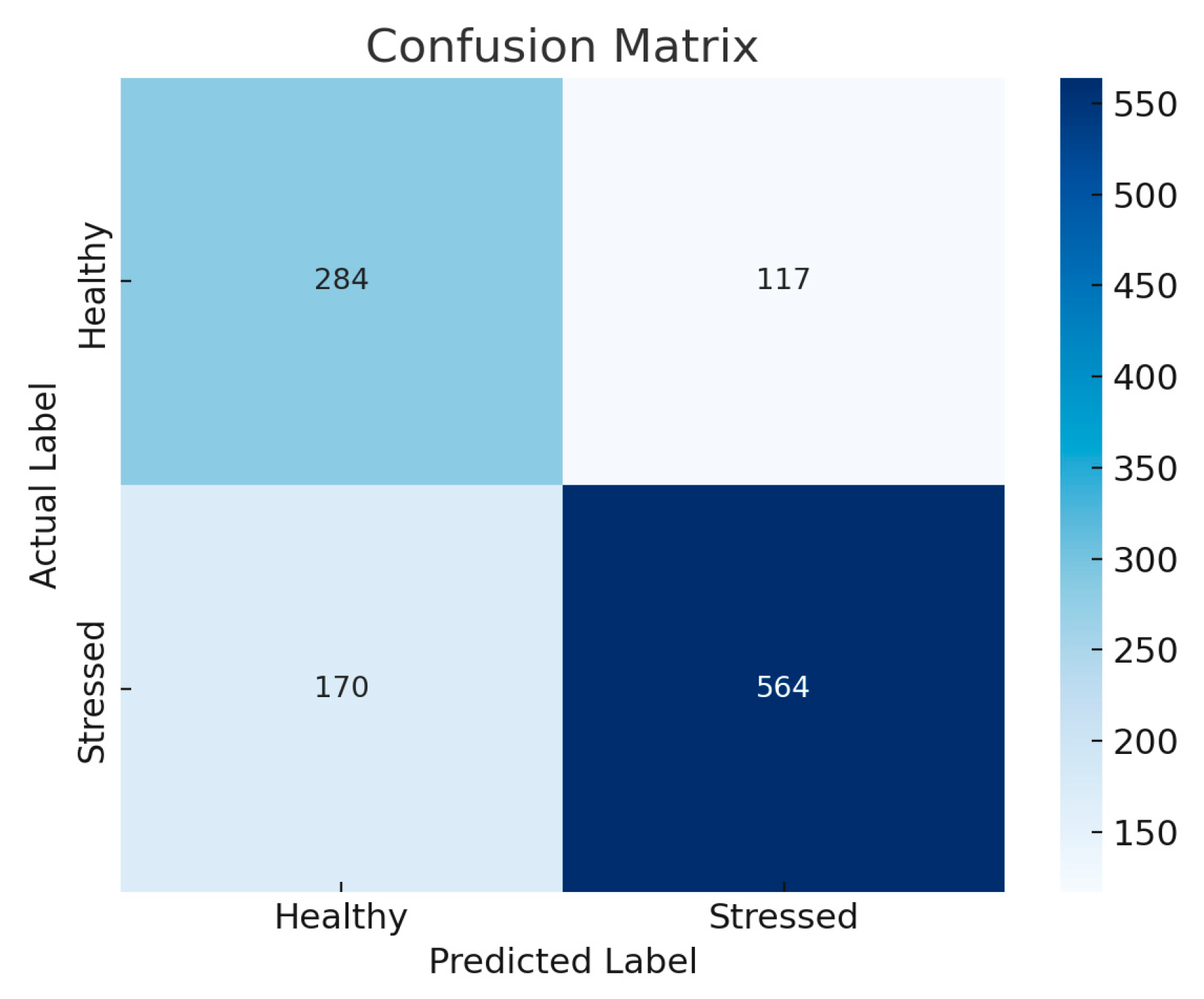
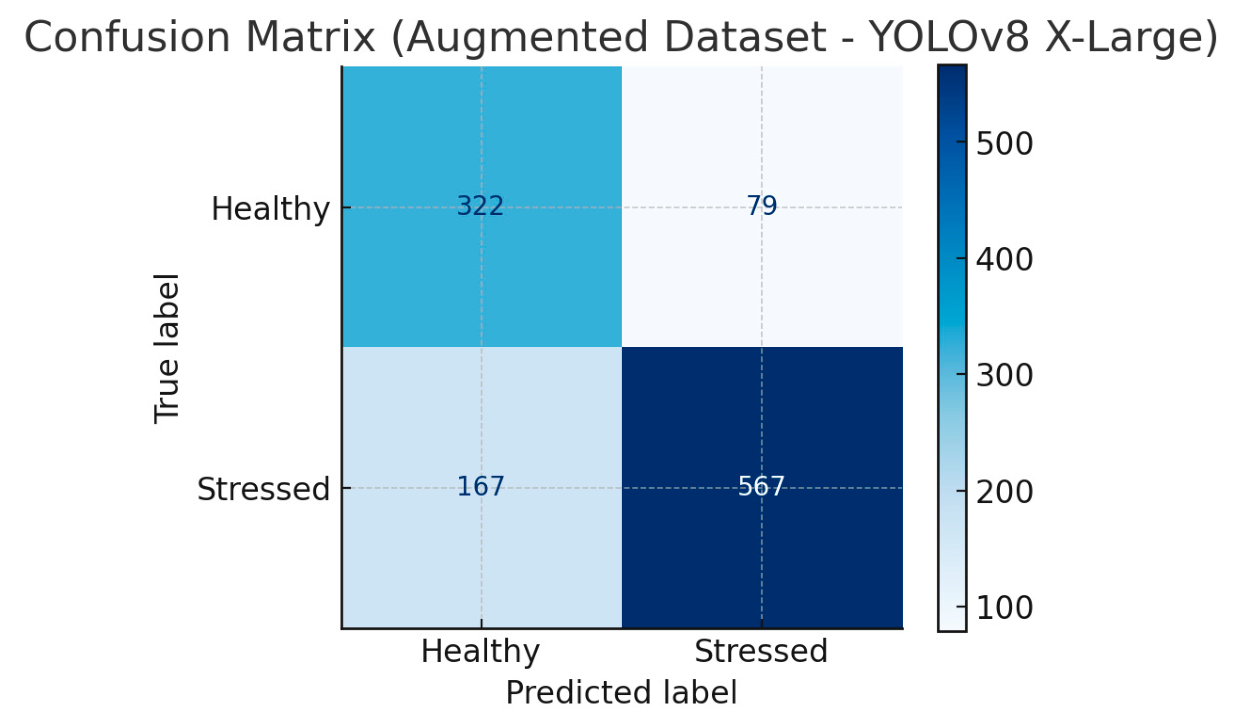
To better understand the results, we generated the confusion matrix for the X-Large YOLOv8 on the original and augmented datasets, as this model has the highest accuracy. Figure 2 shows the confusion matrix for the original dataset, and Figure 3 shows the confusion matrix for the augmented dataset.
The confusion matrices associated with the baseline and augmented datasets clearly illustrate the effect of data augmentation on the model’s performance. In the baseline dataset, the model recorded a precision of 82.8% and a recall of 76.9%, indicating a significant rate of false negatives, especially within the stressed plant class. Following data augmentation, the model’s precision increased to 87.8% and recall to 77.3%, showing reduced false positive and false negative errors and improved overall generalization. The observed increase in correctly identified healthy and stressed plants demonstrates that data augmentation is useful.
To assess these models’ efficiency in making real-time predictions, Table 5 shows the inference time in milliseconds for each YOLOv8 variant on both the original and the augmented datasets. The results show that smaller YOLOv8 variants have lower computational demand. This result also agrees with the findings of [22], which states that YOLOv8 has less computational time than other versions of YOLO, and this makes YOLOv8 suitable for real-time applications.
In our evaluation of the YOLOv8 model variants, we examined their performance across multiple metrics. As shown in Figure 4, we investigated the interplay between mAP@50 for all evaluated variants and inference time for each variant, ranging from the streamlined Nano to the sophisticated X-Large model. Each data point corresponds to a specific YOLOv8 variant.
This combined graph in Figure 4 shows the relationship between the original and augmented datasets for each YOLOv8 variant, where the blue markers represent the original data, and the red markers represent the augmented data. These visualizations provide valuable insights into the trade-offs between model complexity, inference time, and detection accuracy of all YOLOv8 variants. Notably, the X-Large variant achieves the highest mAP@50 score, underscoring its advanced capabilities. As anticipated, the X-Large variant exhibits the longest inference time due to its heightened complexity. The figure also demonstrates that achieving higher mAP@50 values requires increased inference time. These results are consistent with [22] because the performance of YOLO versions depends on the dataset size and image quality. Still, YOLOv8 can achieve high accuracy if we can enhance the dataset inputted to the training process, which means putting more effort into data collection.

4.2. Results of Detection by RetinaNet

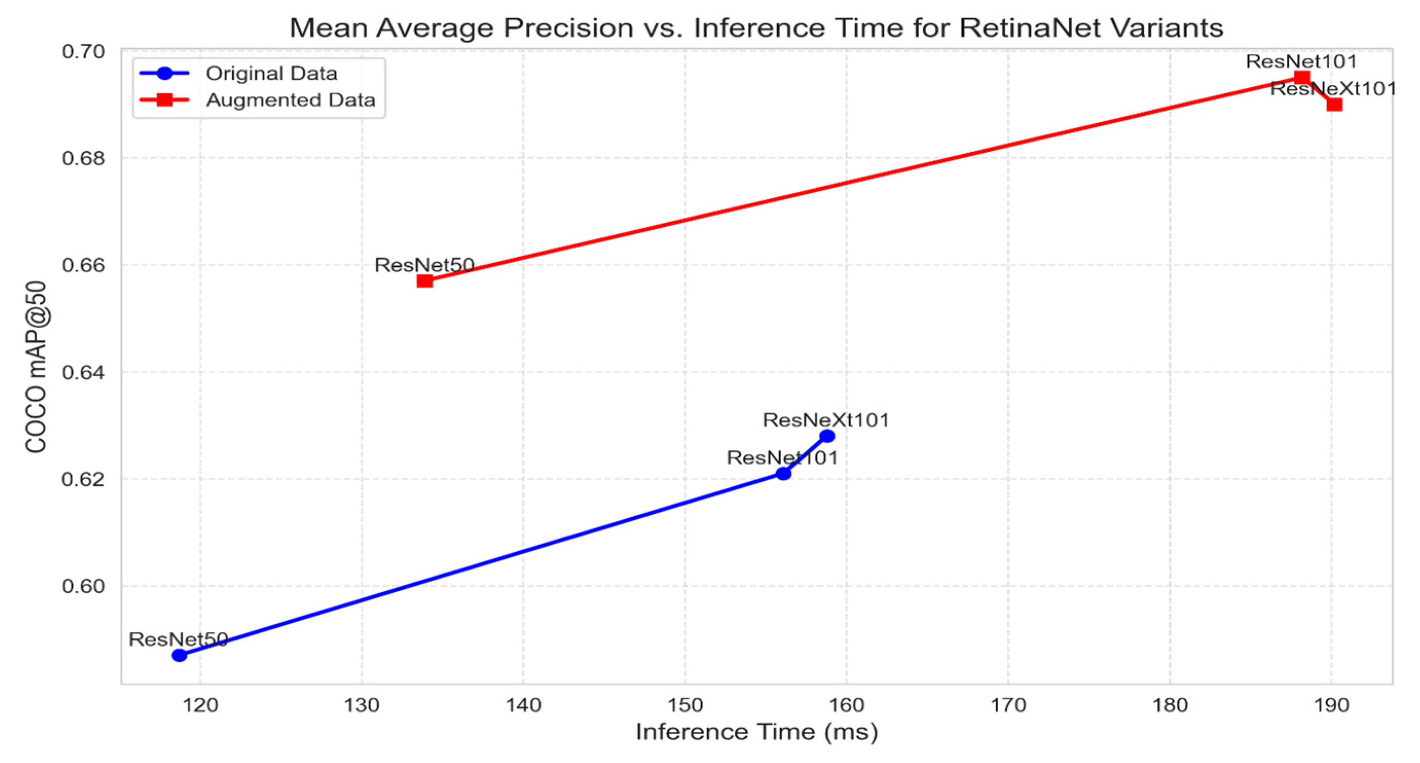
Table 6 presents the performance of RetinaNet variants with different backbones (ResNet50, ResNet101, and ResNeXt101) on the original dataset and the augmented dataset. The three evaluation metrics of mAP provide valuable insights into the model’s capability to accurately detect and classify objects. It is clear that data augmentation increases the accuracy of the RetinaNet models because these models require large datasets. It is also shown that RetinaNet backbones, which are ResNeXt101, are more accurate than the smaller ones.
The inference time for each RetinaNet variant for the original and augmented datasets is shown in Table 7 demonstrating the model’s efficiency in making real-time classifications. The table shows that ResNet50 has the shortest time while the ResNeXt101 backbone variant exhibits the longest inference time due to its high complexity.
Figure 5 illustrates the trade-off between mAP@50 and inference time for the RetinaNet variants on the original and augmented datasets. The blue markers represent the original data, and the red markers represent the augmented data.
As shown in Figure 5, there are trade-offs between each model’s inference time and detection accuracy for RetinaNet. The models achieve higher accuracy on the augmented data than on the original data, as they require a large dataset to perform well.

4.3. Results of Detection by Faster R-CNN

This section presents the evaluation results of Faster R-CNN in crop health assessment. Table 8 shows the performance of Faster R-CNN variants with different backbones (ResNet50, ResNet101, and ResNeXt101) on the original and augmented datasets.
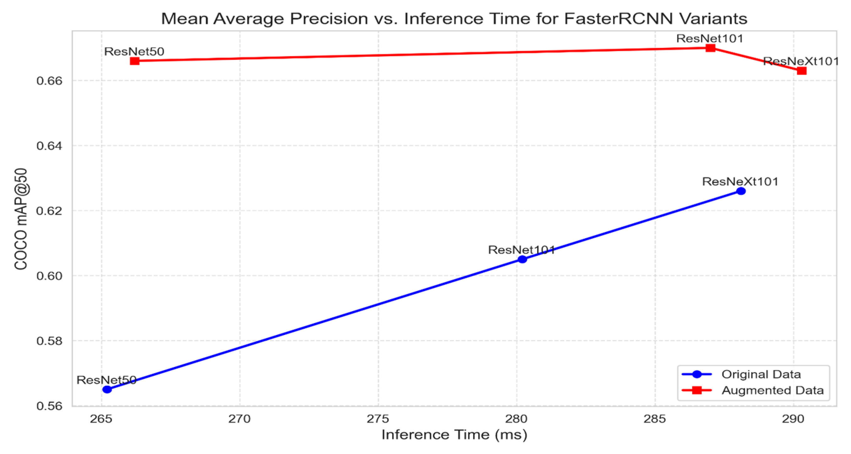
As shown in Table 8, the Faster R-CNN variants achieve higher detection accuracy on the augmented dataset as these models require a large dataset. Similarly to RetinaNet, models with large backbones outperform the smaller ones. The inference time for each Faster R-CNN variant is shown in Table 9 for both datasets, demonstrating their efficiency in real-time predictions. The table shows that the model with the ResNeXt101 backbone exhibits the longest inference time due to its complexity.
Figure 6 shows the performance of each Faster R-CNN variant on the original and augmented datasets. The mAP@50 scores and the inference time for each Faster R-CNN variant on the original and augmented datasets are depicted in the combined graphs below. Red markers represent the augmented data, while blue markers represent the original data.
As shown in Figure 7, it is also clear that there is a trade-off between inference time and mAP@50 for different Faster R-CNN variants. The variants perform better on the augmented dataset than the original dataset in terms of accuracy because Faster R-CNN requires large datasets. However, while accuracy increases linearly when moving from one variant to another on the original data, there are minimal variations across the accuracy values of the variants on the augmented dataset. This makes the ResNet50 variant scale effectively when the number of images is large.

4.4. Comparison

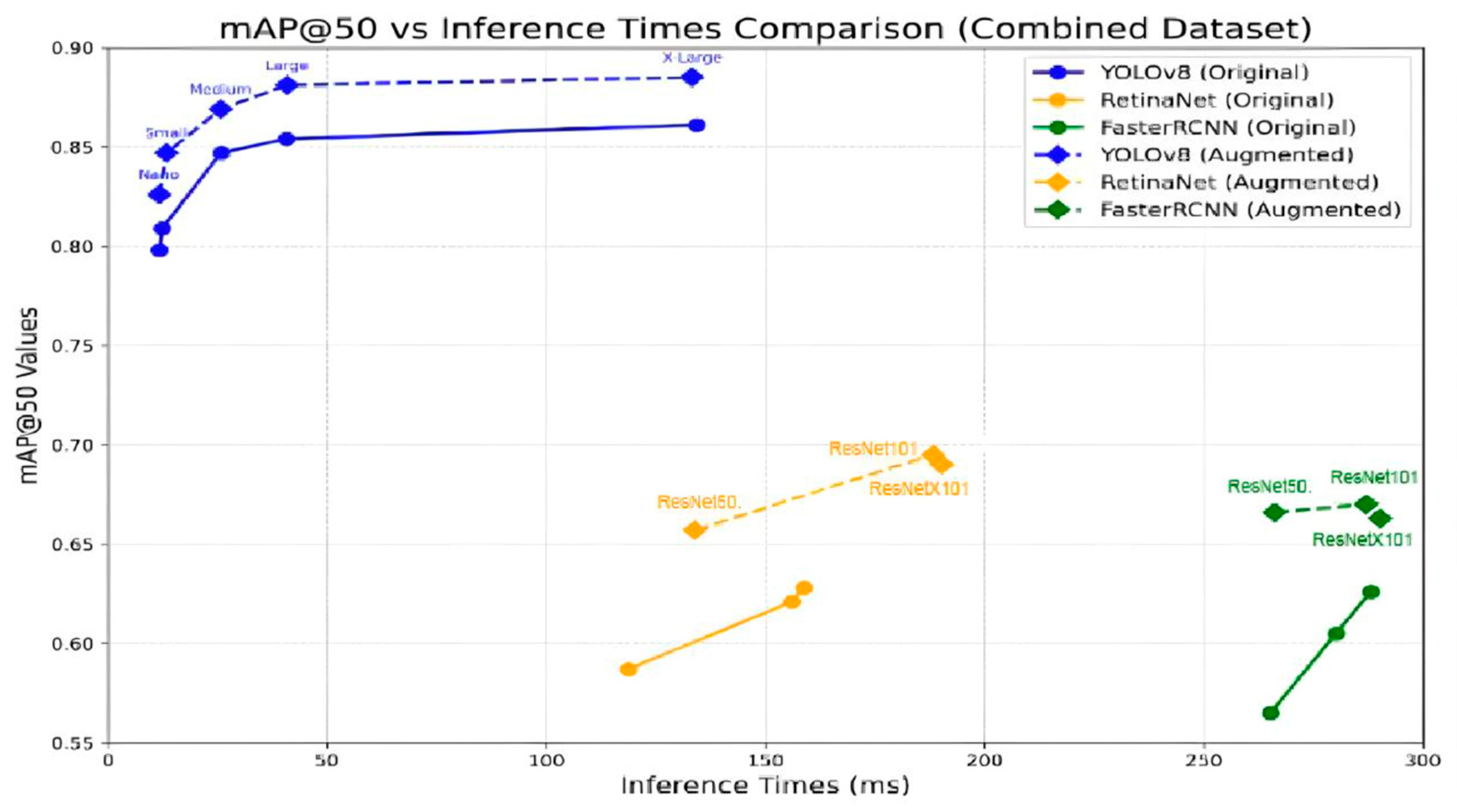
To provide a clearer picture of the results, this section presents a comprehensive comparison of the three object detection models: YOLOv8, RetinaNet, and Faster R-CNN, and their respective variants on both the original and the augmented datasets. Figure 7 shows the relationship between mAP@50 values and inference times for each model and its variants on the original and augmented datasets.
The analysis of the mAP@50 values versus the inference times reveals important insights about the trade-offs between each model’s accuracy and speed. On the original dataset, the results show that RetinaNet and Faster R-CNN achieve comparable mAP@50 values, with small variations depending on the variant type. However, YOLOv8 outperforms both models by exhibiting the highest mAP@50 values across all its variants. It is clear that the YOLOv8-Nano variant not only produces the highest accuracy compared to RetinaNet and Faster R-CNN but also records the smallest inference times, making it well-suited for time-sensitive plant stress detection. While RetinaNet and Faster R-CNN demonstrate competitive accuracy, they require significantly higher inference times, which can limit their practical application to real-time scenarios.
These results highlight a significant balance between accuracy and computational efficiency. The consistently strong performance of YOLOv8 across both datasets demonstrates its reliability and scalability, and suggests that it is the most suitable model among those evaluated for precision agriculture cases using drone imagery. YOLOv8 provides greater accuracy and faster inference time compared to RetinaNet and Faster R-CNN, due to its efficiency and unified architecture. YOLOv8 is a single-stage detector, taking inputs and processing them in one pass. While RetinaNet and Faster R-CNN are both two-stage models that process pixel inputs through a two-stage incremental inference pipeline, YOLOv8 runs inference significantly faster since it eliminates the two-stage steps. YOLOv8 also has a very small-weight version known as YOLOv8-Nano that provides accurate detections while reducing the inference time and computational resources.

5. Conclusions

This research has demonstrated the effectiveness of deep learning models that are YOLOv8, RetinaNet, and Faster R-CNN in analyzing drone-collected images for crop health assessment in precision agriculture. The experiments have found that the YOLOv8 variants outperform the other models as they achieve larger mAP@50 values and lower inference times on both the original and augmented datasets. The YOLOv8 variants achieve mAP@50 ranging from 0.798 to 0.861 and inference times ranging from 11.8 ms to 134.3 ms, while RetinaNet variants achieve mAP@50 ranging from 0.587 to 0.628 and inference times ranging from 118.7 ms to 158.8 ms, and Faster R-CNN variants achieve mAP@50 ranging from 0.587 to 0.628 and inference times ranging from 265 ms to 288 ms.
These results highlight the practical implications of this research, showing that YOLO8 is a robust, lightweight, and scalable method for real-time applications. The results also show that data augmentation techniques enhance model performance and address the common challenge of data deficiency. The proposed method allows for faster and more precise plant stress detection and enables farmers to make data-driven decisions about fertilization, irrigation, and pest control to ultimately improve crop yield and resource management.
The results from this comparison contribute to the possibility of continuous improvement of deep learning models for real-world plant stress detection by experimenting with more advanced methods, such as the Generative R-CNN [57]. Future investigations may also delve deeper into the nuances of data augmentation techniques and their impact on model performance. Further work will also examine how lower-resolution imagery affects accuracy and generalization, and investigate the benefits of incorporating vegetation indices (e.g., NDVI, SAVI) alongside RGB data to improve stress detection under diverse environmental conditions. Additionally, future research can focus on developing applications that use the proposed deep learning model to analyze aerial drone images, providing farmers with insights into crop health, growth patterns, nutrient deficiencies, and pest infestations.

Author Contributions

Conceptualization, Y.-A.D., W.N. and E.Y.D.; Data curation, W.N. and Y.-A.D.; Funding acquisition, E.Y.D. and H.F.; Methodology, Y.-A.D., E.Y.D., W.N. and H.F.; Project administration, E.Y.D.; Software, Y.-A.D. and W.N.; Supervision, H.F.; Validation, E.Y.D. and H.F.; Visualization, Y.-A.D. and W.N.; Writing—original draft, Y.-A.D. and W.N.; Writing—review and editing, Y.-A.D., E.Y.D., W.N. and H.F. All authors have read and agreed to the published version of the manuscript.

Funding

Project Name: AgroChain, Fund name: Al Maqdisi programme, funder: the French-Palestinian Hubert Curien partnership and coordinated by the French Ministry for Europe and Foreign Affairs (MEAE), the French Ministry for Higher Education, Research and Innovation (MESRI), and by the Consulate General of France in Jerusalem.

Data Availability Statement

The original contributions presented in this study are included in the article. Further inquiries can be directed to the corresponding authors.

Acknowledgments

The authors would like to thank Palestine Technical University–Kadoorie (PTUK) and the University de Reims Champagne Ardenne for supporting this research.

Conflicts of Interest

The authors declare no conflict of interest. The funders had no role in the design of the study; in the collection, analyses, or interpretation of data; in the writing of the manuscript; or in the decision to publish the results.

Abbreviations

The following abbreviations are used in this manuscript:
CNNConvolutional Neural Network
DLDeep Learning
MLMachine Learning
YOLOYou Only Look Once
R-CNNRegion-based Convolutional Neural Network
UAVsUnmanned Aerial Vehicles
LSTMLong Short-Term Memory
ResNetResidual Network
mAPMean Average Precision

References

  1. Ning, Y.; Liu, W.; Wang, G.-L. Balancing Immunity and Yield in Crop Plants. Trends Plant Sci. 2017, 22, 1069–1079. [Google Scholar] [CrossRef]
  2. Seelan, S.K.; Laguette, S.; Casady, G.M.; Seielstad, G.A. Remote Sensing Applications for Precision Agriculture: A Learning Community Approach. Remote Sens. Environ. 2003, 88, 157–169. [Google Scholar] [CrossRef]
  3. Akbari, Y.; Almaadeed, N.; Al-Maadeed, S.; Elharrouss, O. Applications, Databases and Open Computer Vision Research from Drone Videos and Images: A Survey. Artif. Intell. Rev. 2021, 54, 3887–3938. [Google Scholar] [CrossRef]
  4. Bilodeau, M.F.; Esau, T.J.; Zaman, Q.U.; Heung, B.; Farooque, A.A. Using Drones to Predict Degradation of Surface Drainage on Agricultural Fields: A Case Study of the Atlantic Dykelands. AgriEngineering 2025, 7, 112. [Google Scholar] [CrossRef]
  5. Miyoshi, K.; Hiraguri, T.; Shimizu, H.; Hattori, K.; Kimura, T.; Okubo, S.; Endo, K.; Shimada, T.; Shibasaki, A.; Takemura, Y. Development of Pear Pollination System Using Autonomous Drones. AgriEngineering 2025, 7, 68. [Google Scholar] [CrossRef]
  6. Toscano, F.; Fiorentino, C.; Santana, L.S.; Magalhães, R.R.; Albiero, D.; Tomáš, Ř.; Klocová, M.; D’Antonio, P. Recent Developments and Future Prospects in the Integration of Machine Learning in Mechanised Systems for Autonomous Spraying: A Brief Review. AgriEngineering 2025, 7, 142. [Google Scholar] [CrossRef]
  7. Kim, H.; Kim, W.; Kim, S.D. Damage Assessment of Rice Crop after Toluene Exposure Based on the Vegetation Index (VI) and UAV Multispectral Imagery. Remote Sens. 2020, 13, 25. [Google Scholar] [CrossRef]
  8. Rábago, J.; Portuguez-Castro, M. Use of Drone Photogrammetry as An Innovative, Competency-Based Architecture Teaching Process. Drones 2023, 7, 187. [Google Scholar] [CrossRef]
  9. Abbas, A.; Zhang, Z.; Zheng, H.; Alami, M.M.; Alrefaei, A.F.; Abbas, Q.; Naqvi, S.A.H.; Rao, M.J.; Mosa, W.F.A.; Abbas, Q.; et al. Drones in Plant Disease Assessment, Efficient Monitoring, and Detection: A Way Forward to Smart Agriculture. Agronomy 2023, 13, 1524. [Google Scholar] [CrossRef]
  10. Martinelli, F.; Scalenghe, R.; Davino, S.; Panno, S.; Scuderi, G.; Ruisi, P.; Villa, P.; Stroppiana, D.; Boschetti, M.; Goulart, L.R.; et al. Advanced Methods of Plant Disease Detection. A Review. Agron. Sustain. Dev. 2015, 35, 1–25. [Google Scholar] [CrossRef]
  11. Meshram, V.; Patil, K.; Meshram, V.; Hanchate, D.; Ramkteke, S.D. Machine Learning in Agriculture Domain: A State-of-Art Survey. Artif. Intell. Life Sci. 2021, 1, 100010. [Google Scholar] [CrossRef]
  12. Gadiraju, K.K.; Ramachandra, B.; Chen, Z.; Vatsavai, R.R. Multimodal Deep Learning Based Crop Classification Using Multispectral and Multitemporal Satellite Imagery. In Proceedings of the 26th ACM SIGKDD International Conference on Knowledge Discovery & Data Mining, Virtual Event, 6–10 July 2020; Association for Computing Machinery: New York, NY, USA, 2020; pp. 3234–3242. [Google Scholar]
  13. Oikonomidis, A.; Catal, C.; Kassahun, A. Deep Learning for Crop Yield Prediction: A Systematic Literature Review. N. Z. J. Crop Hortic. Sci. 2023, 51, 1–26. [Google Scholar] [CrossRef]
  14. Heidari, A.; Jafari Navimipour, N.; Unal, M.; Zhang, G. Machine Learning Applications in Internet-of-Drones: Systematic Review, Recent Deployments, and Open Issues. ACM Comput. Surv. 2023, 55, 1–45. [Google Scholar] [CrossRef]
  15. Geetha, V.; Punitha, A.; Abarna, M.; Akshaya, M.; Illakiya, S.; Janani, A. An Effective Crop Prediction Using Random Forest Algorithm. In Proceedings of the 2020 International Conference on System, Computation, Automation and Networking (ICSCAN), Pondicherry, India, 3–4 July 2020; pp. 1–5. [Google Scholar]
  16. Nalini, T.; Rama, A. Impact of Temperature Condition in Crop Disease Analyzing Using Machine Learning Algorithm. Meas. Sens. 2022, 24, 100408. [Google Scholar] [CrossRef]
  17. Nishankar, S.; Pavindran, V.; Mithuran, T.; Nimishan, S.; Thuseethan, S.; Sebastian, Y. ViT-RoT: Vision Transformer-Based Robust Framework for Tomato Leaf Disease Recognition. AgriEngineering 2025, 7, 185. [Google Scholar] [CrossRef]
  18. Wang, J.; Li, J.; Meng, F. Recognition of Strawberry Powdery Mildew in Complex Backgrounds: A Comparative Study of Deep Learning Models. AgriEngineering 2025, 7, 182. [Google Scholar] [CrossRef]
  19. Dang, L.M.; Wang, H.; Li, Y.; Min, K.; Kwak, J.T.; Lee, O.N.; Park, H.; Moon, H. Fusarium Wilt of Radish Detection Using RGB and Near Infrared Images from Unmanned Aerial Vehicles. Remote Sens. 2020, 12, 2863. [Google Scholar] [CrossRef]
  20. Su, J.; Yi, D.; Su, B.; Mi, Z.; Liu, C.; Hu, X.; Xu, X.; Guo, L.; Chen, W.-H. Aerial Visual Perception in Smart Farming: Field Study of Wheat Yellow Rust Monitoring. IEEE Trans. Ind. Inform. 2021, 17, 2242–2249. [Google Scholar] [CrossRef]
  21. Shah, S.A.; Lakho, G.M.; Keerio, H.A.; Sattar, M.N.; Hussain, G.; Mehdi, M.; Vistro, R.B.; Mahmoud, E.A.; Elansary, H.O. Application of Drone Surveillance for Advance Agriculture Monitoring by Android Application Using Convolution Neural Network. Agronomy 2023, 13, 1764. [Google Scholar] [CrossRef]
  22. Zhao, S.; Chen, H.; Zhang, D.; Tao, Y.; Feng, X.; Zhang, D. SR-YOLO: Spatial-to-Depth Enhanced Multi-Scale Attention Network for Small Target Detection in UAV Aerial Imagery. Remote Sens. 2025, 17, 2441. [Google Scholar] [CrossRef]
  23. Fuentes, A.; Yoon, S.; Kim, S.C.; Park, D.S. A Robust Deep-Learning-Based Detector for Real-Time Tomato Plant Diseases and Pests Recognition. Sensors 2017, 17, 2022. [Google Scholar] [CrossRef] [PubMed]
  24. Hamidisepehr, A.; Mirnezami, S.V.; Ward, J.K. Comparison of Object Detection Methods for Corn Damage Assessment Using Deep Learning. Trans. ASABE 2020, 63, 1969–1980. [Google Scholar] [CrossRef]
  25. Butte, S.; Vakanski, A.; Duellman, K.; Wang, H.; Mirkouei, A. Potato Crop Stress Identification in Aerial Images Using Deep Learning-based Object Detection. Agron. J. 2021, 113, 3991–4002. [Google Scholar] [CrossRef]
  26. Dawod, R.G.; Dobre, C. Upper and Lower Leaf Side Detection with Machine Learning Methods. Sensors 2022, 22, 2696. [Google Scholar] [CrossRef]
  27. Hughes, D.; Salathé, M. An Open Access Repository of Images on Plant Health to Enable the Development of Mobile Disease Diagnostics. arXiv 2015, arXiv:1511.08060. [Google Scholar]
  28. Amarasingam, N.; Ashan Salgadoe, A.S.; Powell, K.; Gonzalez, L.F.; Natarajan, S. A Review of UAV Platforms, Sensors, and Applications for Monitoring of Sugarcane Crops. Remote Sens. Appl. Soc. Environ. 2022, 26, 100712. [Google Scholar] [CrossRef]
  29. Zhang, T.; Xu, Z.; Su, J.; Yang, Z.; Liu, C.; Chen, W.-H.; Li, J. Ir-UNet: Irregular Segmentation U-Shape Network for Wheat Yellow Rust Detection by UAV Multispectral Imagery. Remote Sens. 2021, 13, 3892. [Google Scholar] [CrossRef]
  30. Barbosa Júnior, M.R.; Santos, R.G.D.; Sales, L.D.A.; Martins, J.V.D.S.; Santos, J.G.D.A.; Oliveira, L.P.D. Designing and Implementing a Ground-Based Robotic System to Support Spraying Drone Operations: A Step Toward Collaborative Robotics. Actuators 2025, 14, 365. [Google Scholar] [CrossRef]
  31. Yadav, S.S.; Jadhav, S.M. Deep Convolutional Neural Network Based Medical Image Classification for Disease Diagnosis. J. Big Data 2019, 6, 113. [Google Scholar] [CrossRef]
  32. Fatih, B.; Kayaalp, F. Review of Machine Learning and Deep Learning Models in Agriculture. Int. Adv. Res. Eng. J. 2021, 5, 309–323. [Google Scholar] [CrossRef]
  33. Sarker, I.H. Deep Learning: A Comprehensive Overview on Techniques, Taxonomy, Applications and Research Directions. SN Comput. Sci. 2021, 2, 420. [Google Scholar] [CrossRef]
  34. Kamilaris, A.; Prenafeta-Boldú, F.X. Deep Learning in Agriculture: A Survey. Comput. Electron. Agric. 2018, 147, 70–90. [Google Scholar] [CrossRef]
  35. Latha, R.S.; Sreekanth, G.R.; Suganthe, R.C.; Geetha, M.; Swathi, N.; Vaishnavi, S.; Sonasri, P. Automatic Fruit Detection System Using Multilayer Deep Convolution Neural Network. In Proceedings of the 2021 International Conference on Computer Communication and Informatics (ICCCI), Coimbatore, India, 27–29 January 2021; IEEE: Coimbatore, India, 2021; pp. 1–5. [Google Scholar]
  36. Ramos-Giraldo, P.; Reberg-Horton, C.; Locke, A.M.; Mirsky, S.; Lobaton, E. Drought Stress Detection Using Low-Cost Computer Vision Systems and Machine Learning Techniques. IT Prof. 2020, 22, 27–29. [Google Scholar] [CrossRef]
  37. An, J.; Li, W.; Li, M.; Cui, S.; Yue, H. Identification and Classification of Maize Drought Stress Using Deep Convolutional Neural Network. Symmetry 2019, 11, 256. [Google Scholar] [CrossRef]
  38. Tran, T.-T.; Choi, J.-W.; Le, T.-T.H.; Kim, J.-W. A Comparative Study of Deep CNN in Forecasting and Classifying the Macronutrient Deficiencies on Development of Tomato Plant. Appl. Sci. 2019, 9, 1601. [Google Scholar] [CrossRef]
  39. Anami, B.S.; Malvade, N.N.; Palaiah, S. Classification of Yield Affecting Biotic and Abiotic Paddy Crop Stresses Using Field Images. Inf. Process. Agric. 2020, 7, 272–285. [Google Scholar] [CrossRef]
  40. Albahli, S. 5: A Lightweight Deep Learning Model for Multisource Plant Disease Diagnosis. Agriculture 2025, 15, 1523. [Google Scholar] [CrossRef]
  41. Mohanty, S.P.; Hughes, D.P.; Salathé, M. Using Deep Learning for Image-Based Plant Disease Detection. Front. Plant Sci. 2016, 7, 1419. [Google Scholar] [CrossRef] [PubMed]
  42. Amara, J.; Bouaziz, B.; Algergawy, A. A Deep Learning-Based Approach for Banana Leaf Diseases Classification. Agric. Food Sci. Comput. Sci. 2017, 1, 79. [Google Scholar]
  43. Ramcharan, A.; Baranowski, K.; McCloskey, P.; Ahmed, B.; Legg, J.; Hughes, D.P. Deep Learning for Image-Based Cassava Disease Detection. Front. Plant Sci. 2017, 8, 1852. [Google Scholar] [CrossRef]
  44. Yamamoto, K.; Togami, T.; Yamaguchi, N. Super-Resolution of Plant Disease Images for the Acceleration of Image-Based Phenotyping and Vigor Diagnosis in Agriculture. Sensors 2017, 17, 2557. [Google Scholar] [CrossRef]
  45. Liu, B.; Zhang, Y.; He, D.; Li, Y. Identification of Apple Leaf Diseases Based on Deep Convolutional Neural Networks. Symmetry 2017, 10, 11. [Google Scholar] [CrossRef]
  46. Ghosal, S.; Blystone, D.; Singh, A.K.; Ganapathysubramanian, B.; Singh, A.; Sarkar, S. An Explainable Deep Machine Vision Framework for Plant Stress Phenotyping. Proc. Natl. Acad. Sci. USA 2018, 115, 4613–4618. [Google Scholar] [CrossRef]
  47. Rançon, F.; Bombrun, L.; Keresztes, B.; Germain, C. Comparison of SIFT Encoded and Deep Learning Features for the Classification and Detection of Esca Disease in Bordeaux Vineyards. Remote Sens. 2018, 11, 1. [Google Scholar] [CrossRef]
  48. Tian, H.; Wang, P.; Tansey, K.; Zhang, J.; Zhang, S.; Li, H. An LSTM Neural Network for Improving Wheat Yield Estimates by Integrating Remote Sensing Data and Meteorological Data in the Guanzhong Plain, PR China. Agric. For. Meteorol. 2021, 310, 108629. [Google Scholar] [CrossRef]
  49. Dharani, M.K.; Thamilselvan, R.; Natesan, P.; Kalaivaani, P.; Santhoshkumar, S. Review on Crop Prediction Using Deep Learning Techniques. J. Phys. Conf. Ser. 2021, 1767, 012026. [Google Scholar] [CrossRef]
  50. Koirala, A.; Walsh, K.; Wang, Z.; McCarthy, C. Deep Learning for Real-Time Fruit Detection and Orchard Fruit Load Estimation: Benchmarking of ‘MangoYOLO’. Precis. Agric. 2019, 20, 1107–1135. [Google Scholar] [CrossRef]
  51. Villacrés, J.F.; Auat Cheein, F. Detection and Characterization of Cherries: A Deep Learning Usability Case Study in Chile. Agronomy 2020, 10, 835. [Google Scholar] [CrossRef]
  52. Chi, H.-C.; Sarwar, M.A.; Daraghmi, Y.-A.; Lin, K.-W.; Ik, T.-U.; Li, Y.-L. Smart Self-Checkout Carts Based on Deep Learning for Shopping Activity Recognition. In Proceedings of the 2020 21st Asia-Pacific Network Operations and Management Symposium (APNOMS), Daegu, Republic of Korea, 22–25 September 2020; IEEE: Piscataway, NJ, USA, 2020; pp. 185–190. [Google Scholar]
  53. Sarwar, M.A.; Daraghmi, Y.-A.; Liu, K.-W.; Chi, H.-C.; Ik, T.-U.; Li, Y.-L. Smart Shopping Carts Based on Mobile Computing and Deep Learning Cloud Services. In Proceedings of the 2020 IEEE Wireless Communications and Networking Conference (WCNC), Seoul, Republic of Korea, 25–28 May 2020; IEEE: Piscataway, NJ, USA, 2020; pp. 1–6. [Google Scholar]
  54. Yaseen, M. What is YOLOv8: An in-Depth Exploration of the Internal Features of the Next-Generation Object Detector. arXiv 2024, arXiv:2408.15857. [Google Scholar]
  55. Lin, T.-Y.; Goyal, P.; Girshick, R.; He, K.; Dollár, P. Focal Loss for Dense Object Detection. In Proceedings of the IEEE International Conference on Computer Vision (ICCV), Venice, Italy, 22–29 October 2017; pp. 2980–2988. [Google Scholar]
  56. Ren, S.; He, K.; Girshick, R.; Sun, J. Faster R-CNN: Towards Real-Time Object Detection with Region Proposal Networks. IEEE Trans. Pattern Anal. Mach. Intell. 2017, 39, 1137–1149. [Google Scholar] [CrossRef] [PubMed]
  57. Saffarini, R.; Khamayseh, F.; Awwad, Y.; Sabha, M.; Eleyan, D. Dynamic Generative R-CNN. Neural Comput. Appl. 2025, 37, 7107–7120. [Google Scholar] [CrossRef]
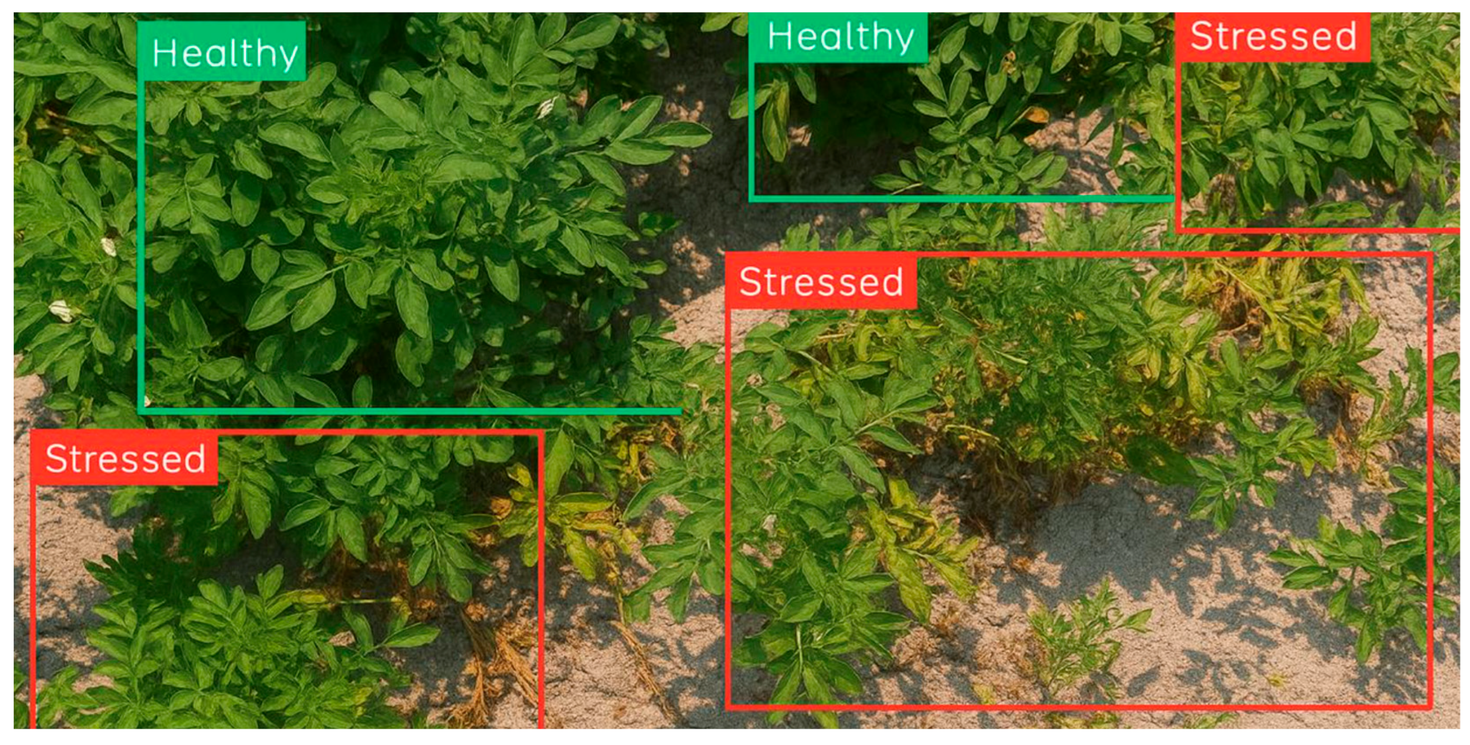
Figure 1. Sample images from the original dataset showing the healthy plants in green boxes and stressed plants in red boxes.
Agriengineering 07 00257 g001
Figure 2. The confusion matrix for the X-Large YOLOv8 on the original dataset.
Agriengineering 07 00257 g002
Figure 3. The confusion matrix for the X-Large YOLOv8 on the augmented dataset.
Agriengineering 07 00257 g003
Figure 4. Mean Average Precision (mAP@50) vs. Inference Time for YOLOv8 variants for both the original and augmented datasets showing that the augmented data produce higher accuracy but with higher computational time.
Agriengineering 07 00257 g004
Figure 5. Mean Average Precision vs. inference time for RetinaNet variants.
Agriengineering 07 00257 g005
Figure 6. Mean average precision vs. inference time for Faster R-CNN variants.
Agriengineering 07 00257 g006
Figure 7. Mean average precision vs. inference time comparison for all models on the original and augmented datasets.
Agriengineering 07 00257 g007
Table 1. Most related deep learning models and their performance.
Ref.ContextMethodEvaluation
Metric
ValueInference Time
[25]Potato stress detectionRatina-UNetDice score coefficient (DSC)74%NA
[19]Fusarium Wilt of Radish DetectionCustomized deep learningRecall96.0%NA
[21]Advanced Agriculture MonitoringEfficientNet-B3
(modified CNN)
Precision97.0%NA
[42]Leaf disease detectionResNet125Recall85.0%NA
[29]Wheat yellow rust detectionIr-UnetRecall95.0%NA
[38]Macronutrient Deficiencies on Development of Tomato PlantInception-ResNetRecall91.22%NA
[39]biotic and abiotic addy crop stressesBack Propagation Neural Network (BPNN)Accuracy89.12%NA
[24]Corn damage assessmentYOLOv2Precision97.0%NA
[24]Corn damage assessmentFaster R-CNNPrecision77.29%NA
[24]Corn damage assessmentRetinaNetPrecision93.87%NA
[40]Multisource plant disease diagnosisAgriFusionNetPrecision94.1%28.5
Table 2. Bounding Box Scale Distribution in the original Dataset.
Class NameSmall ScaleMedium ScaleLarge ScaleTotal
Healthy1812216132041
Stressed293118603117
Total4743402135158
Table 3. Class distribution—The number of healthy and stressed plants in the original and augmented datasets.
Dataset SubsetHealthyStressedTotal
Training original data164023844024
Training augmented data820011,92020,120
Testing4017341135
Table 4. Performance of YOLOv8 variants on the original and augmented datasets.
YOLOv8 VariantPrecisionRecallmAP@50mAP@50–95
NanoOriginal dataset0.7540.7380.7980.619
Nano—Augmented dataset0.8060.740.8260.719
Small—Original dataset0.7580.7480.8090.661
Small—Augmented dataset0.7870.7920.8470.771
Medium—Original dataset0.8170.7440.8470.73
Medium—Augmented dataset0.8650.7640.8690.796
Large—Original dataset0.8210.7750.8540.75
Large—Augmented dataset0.8360.8050.8810.819
X-Large—Original dataset0.8280.7690.8610.763
X-Large—Augmented dataset0.8780.7730.8850.82
Table 5. Inference time of YOLOv8 on the original and augmented datasets.
YOLOv8 VariantInference Time (ms)
Original Dataset
Inference Time (ms)
Augmented Dataset
Nano11.811.7
Small12.413.4
Medium25.825.7
Large40.740.9
X-Large134.3133.3
Table 6. Accuracy of RetinaNet variants on the original and augmented datasets.
RetinaNet VariantmAP@50mAP@75mAP@50–95
ResNet50—Original dataset0.5870.3190.339
ResNet50—Augmented dataset0.6570.420.43
ResNet101—Original dataset0.6210.3540.362
ResNet101—Augmented dataset0.6950.460.467
ResNeXt101—Original dataset0.6280.3640.368
ResNeXt101—Augmented dataset0.690.460.466
Table 7. Inference time of RetinaNet variants on the original and augmented datasets.
ModelInference Time (ms)
Original Dataset
Inference Time (ms)
Augmented Dataset
ResNet50118.7133.9
ResNet101156.1188.2
ResNeXt101158.8190.2
Table 8. Accuracy of Faster R-CNN variants on the original and augmented datasets.
Faster RCNN VariantmAP@50mAP@75mAP@50–95
ResNet50—Original dataset0.5650.2780.293
ResNet50—Augmented dataset0.6660.4050.411
ResNet101—Original dataset0.6050.3670.366
ResNet101—Augmented dataset0.670.4670.464
ResNeXt101—Original dataset0.6260.3910.381
ResNeXt101—Augmented dataset0.6630.4520.457
Table 9. Inference time of Faster R-CNN variants on the original and augmented datasets.
ModelInference Time (ms)
Original Dataset
Inference Time (ms)
Augmented Dataset
ResNet50265.2266.2
ResNet101280.2287.0
ResNeXt101288.1290.3
Disclaimer/Publisher’s Note: The statements, opinions and data contained in all publications are solely those of the individual author(s) and contributor(s) and not of MDPI and/or the editor(s). MDPI and/or the editor(s) disclaim responsibility for any injury to people or property resulting from any ideas, methods, instructions or products referred to in the content.