Abstract
This study proposes CEL-DL-Bagging (Cross-Entropy Loss-optimized Deep Learning Bagging), a multi-model fusion framework that integrates cross-entropy loss-weighted voting with Bootstrap Aggregating (Bagging). First, we develop a lightweight recognition architecture by embedding a salient position attention (SPA) mechanism into four base networks (YOLOv5s-cls, EfficientNet-B0, MobileNetV3, and ShuffleNetV2), significantly enhancing discriminative feature extraction for disease patterns. Our experiments show that these SPA-enhanced models achieve consistent accuracy gains of 0.8–1.7 percentage points, peaking at 97.86%. Building on this, we introduce DB-CEWSV—an ensemble framework combining Deep Bootstrap Aggregating (DB) with adaptive Cross-Entropy Weighted Soft Voting (CEWSV). The system dynamically optimizes model weights based on their cross-entropy performance, using SPA-augmented networks as base learners. The final integrated model attains 98.33% accuracy, outperforming the strongest individual base learner by 0.48 percentage points. Compared with single models, the ensemble learning algorithm proposed in this study led to better generalization and robustness of the ensemble learning model and better identification of rice diseases in the natural background. It provides a technical reference for applying rice disease identification in practical engineering.
1. Introduction
Rice cultivation has long occupied an important place in agricultural development. However, ill-defined agricultural production patterns and changing climatic environments have affected the yield, quality, and food security of rice cultivation. Plant phenotypes are physical, physiological, and biochemical characteristics that reflect the structural and functional features of plant cells, tissues, organs, plants, and communities [1]. Plant diseases, as important indicators of morphological and structural characteristics of plant phenotypes, can be directly accessed by visible light cameras (including cell phones, digital cameras, etc.) [2]. Rice leaf disease identification is an important research component in the field of plant protection, and efficient disease identification is a major challenge for breeders. Traditional identification methods rely on manual diagnosis by agronomists or disease mapping comparisons. However, due to the complexity and similarity of rice disease spots, manual identification requires extensive experience and agricultural knowledge. This method is extremely demanding for breeders, but it is difficult to provide a large number of specialized human resources in practice. Therefore, intelligent planting combining computer vision, image processing, machine learning (ML), and deep learning (DL) algorithms has attracted much attention. Compared with the artificial vision-based recognition model, this method automatically identifies rice diseases by learning their phenotypic characteristics, which helps farmers to detect, diagnose, and treat the diseases in time at the early stage of disease occurrence, and to seize the best time for prevention and treatment [3].
Previous machine learning disease recognition research incorporating image processing techniques achieved great success, but the method still relied on manual feature extraction [4]. The emergence of deep learning has broken this limitation, and its ability to automatically learn features and reasoning has achieved a major breakthrough in plant disease phenotype recognition applications. A convolutional neural network (CNN), as a representative deep learning technology, performs far better than other traditional recognition methods in image recognition. Lu et al. [5] applied a CNN to rice disease recognition research for the first time, and found that CNNs have better convergence and recognition accuracy than other algorithms, such as the standard BP algorithm, Support Vector Machines (SVMs), and Particle Swarm Optimization (PSO). Jiang et al. [6] combined a CNN and an SVM to improve the recognition performance of rice leaf diseases using a 10-fold cross-validation method. Hu et al. [7] proposed a multi-scale two-branch structured rice pest recognition model based on a generative adversarial network and improved ResNet, which solved the problems of overfitting caused by a too-small dataset and the difficulty of extracting disease features from the background of the picture.
CNN-based rice disease recognition in simple contexts has achieved high accuracy, but there are fewer applications in natural contexts. The most important reason for that is that CNNs are too complex to be deployed on hardware devices, so the application of lightweight networks is necessary. Cai et al. [8] designed a corn leaf disease recognition application based on improved EfficientNet with 3.44 M parameters and 339.74 M Flops, which can be quickly deployed and recognized on Android devices. Butera et al. [9] investigated baseline crop pest detection models that can be applied to real scenarios, taking into account the detection performance and computational resources, in which FasterRCNN with MobileNetV3 as the backbone was outstanding in terms of accuracy and real-time performance. Zhou et al. [10] proposed a lightweight ShuffleNetV2-based crop leaf disease recognition model, which achieved 96.72% accuracy on a field crop leaf disease dataset, with a smaller model size for easy mobile deployment. The above lightweight network model has been widely used to meet the application conditions in natural scenarios.
You Only Look Once (YOLO) is currently a widely used lightweight target detection network. The Ultralytics team released YOLOv5-cls [11], an improved classification model based on YOLOv5, in 2022, comprising five versions. Compared to other traditional CNNs trained on the ImageNet dataset, YOLOv5-cls has practical applications as a lightweight model that ensures model accuracy and reduces parameters. Yang et al. [12] applied YOLOv5-cls for the first time to a real-world classification task, comparing the different versions of the free-roaming bird behavioral classification task on the EfficientNetV2 and YOLOv5-cls, of which YOLOv5m-cls performed best with an average accuracy of 95.3%.
Traditional model training requires constant parameter tuning and a large number of uniformly distributed datasets to obtain efficient models. Currently, it is difficult to construct large-scale, uniform, and high-quality datasets in practical engineering. Transfer learning realizes cross-domain knowledge migration by adapting feature information from pre-trained models to new tasks [13]. When resources and data are limited, this method can effectively reduce data volume requirements and computational costs, and improve the diagnostic and error-correction capabilities of the model. Hassan et al. [14] applied transfer learning to MobileNetV2 and EfficientNet-B0 models by freezing the weights of the models before the fully connected layer and training them to achieve the recognition of multiple plant diseases. Zhao et al. [15] used a model pre-trained on the large dataset ImageNET to initialize the network weight parameters, and the method achieved 92.00% accuracy in recognizing rice plant images. Chen et al. [16] used the PlantVillage dataset for model pre-training, and then fine-tuned the model parameters and applied them to the training of the cotton disease image dataset, achieving an accuracy of 97.16% accuracy. Wang et al. [17] proposed a backbone network based on improved SwinT combined with transfer learning to train a cucumber leaf disease recognition model with 98.97% accuracy. Yuan et al. [18] proposed a framework for rice disease phenotype recognition in a natural context based on transfer learning and SENet with attention policy on a cloud platform that achieved an accuracy rate of 95.73%.
The currently studied rice disease recognition models still face many challenges when facing real field environments. Different deep learning models have different feature extraction strategies, and it is difficult to construct generalized models to achieve optimal recognition performance for various diseases in natural contexts. Therefore, researchers have introduced integrated learning into crop disease recognition [19]. Xu et al. [20] constructed a tomato pest and disease diagnostic model based on Stacking integrated learning, with a diagnostic accuracy of 94.84% and a reduction in inference time of 12.08%. Mathew et al. [21] analyzed the symptoms of plant leaves using the GLCM algorithm and used simple integrated learning techniques such as voting strategies for disease identification. In addition, deep integrated learning models [22] combine the advantages of deep learning models and integrated learning with better recognition performance and generalization ability. Palanisamy et al. [23] used Sequence2D and DenseNet deep learning models combined with integrated learning techniques such as weighted voting strategies for maize leaf infection identification. Yang et al. [24] proposed a Stacking-based deep integrated learning model integrating an improved CNN and using SVM for rice leaf disease recognition.
Some of the above studies introduced integrated learning based on voting strategies into crop disease recognition, which effectively improved the recognition accuracy. However, rice leaf disease recognition under natural background is susceptible to light angle, light intensity, and shading, and there are fewer models available for practical applications. The existing rice leaf disease dataset under a natural background is small and difficult to construct. The stability and generalization ability of deep CNNs on small datasets are difficult to balance.
We propose CEL-DL-Bagging, an integrated learning algorithm combining deep learning (DL) and Bootstrap aggregation (Bagging)-based aggregation, for small-sample rice leaf disease recognition in natural contexts. Four lightweight CNNs are selected as base learners, including YOLOv5-cls, EfficientNet-B0 [25], MobileNetV3 [26], and ShuffleNetV2 [27], to reduce the computational cost while extracting rice leaf disease phenotypic features more comprehensively. Transfer learning was used to train the model to minimize the effect of insufficient data volume. A new CEL-based weighted voting strategy is proposed for disease identification to improve the identification accuracy. In addition, a salient position-based attention mechanism (SPA) is introduced in this paper to further improve the base learner’s ability to extract valid information in complex backgrounds. The method has the following five main contributions:
- (1)
- A rice disease recognition algorithm based on salient positions attention (SPA) mechanism was designed, which reduces the processing of non-critical information.
- (2)
- The DL-Bagging algorithm was proposed, and the lightweight model is integrated by using Bootstrap sampling to improve the generalization ability under small sample sizes.
- (3)
- A CEL-based weighted voting strategy was proposed to improve the DL-Bagging algorithm, and the weights were dynamically adjusted according to the model performance to improve the integration accuracy.
- (4)
- An improved method was proposed that uses the label smoothing technique and cosine annealing strategy in transfer learning training.
- (5)
- A large number of ablation experiments were designed to validate the performance of the proposed method in rice leaf disease recognition under natural backgrounds.
The method proposed in this paper can be applied to real fields to effectively recognize rice leaf diseases in a natural context. The rest of the paper is structured as follows: Section 2 describes the image acquisition, preprocessing, model construction, parameter settings, and evaluation metrics; Section 3 analyzes the results of the experiments; Section 4 discusses the advantages and limitations of the model we are currently using compared to other related studies; and Section 5 concludes the whole paper and looks into the future.
2. Materials and Methods
2.1. Image Acquisition
The data used in this study were partially sourced from the experimental fields for the construction of green, high-yield, and efficient rice fields in Yangzhou City, Jiangsu Province, and supplemented with data from the Elsevier Mendeley database and the public database Kaggle. To ensure the diversity and representativeness of the dataset, images were captured at different times of the day and under varying environmental conditions, including changes in lighting and humidity. Images were captured using an iPhone 15 Pro Max at the experimental field. Blurry, blurred, distorted, or images with unknown diseases or missing features were manually removed. The filtered images were uniformly saved in JPG format, and each image was subjected to multiple local cropping using Photoshop, resulting in 332 sample images. Rice leaf disease images were classified into five categories based on disease type: bacterial leaf blight, rice blast, brown spot disease, tungro disease, and healthy leaves. Each category was stored in a separate folder. Since model training typically requires a large amount of uniformly distributed data to effectively avoid overfitting and poor accuracy, an additional 2546 images were screened from public databases Mendeley Data and Kaggle as supplementary data. Finally, a rice disease dataset comprising 2878 sample images was obtained, completing the construction of the dataset used in this study. Figure 1 illustrates the rice disease samples.
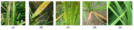
Figure 1.
The rice disease samples. (a) Bacterial leaf blight, (b) rice blast, (c) brown spot, (d) tungro, (e) health.
2.2. Image Preprocessing and Expansion
In order to improve the generalization ability of the model to the shooting angle, light intensity and light angle in the real environment, this paper carries out data enhancement operations such as flipping, rotating, color enhancement, brightness enhancement, contrast enhancement, and randomly transforming the color of the rice disease sample images, and finally obtains the rice disease dataset consisting of 6090 sample images. Table 1 shows the distribution of the rice disease image dataset before and after expansion, and Figure 2 demonstrates the effect of data enhancement on the rice disease sample images after completing the data enhancement. In addition, the image sizes from different sources are inconsistent, and to ensure the validity of the experiment, the image size is standardized to 224 × 224. Finally, to verify the enhancement effect of the model’s generalization ability, 840 disease images with feature information that differs greatly from other images are manually screened as the test set, and the remaining 5250 images are randomly divided into the training set and the validation set according to a ratio of 8:2.

Table 1.
Rice disease dataset.
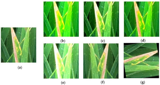
Figure 2.
Data augmentation operations. (a) Original map, (b)random colors, (c) contrast, (d) color, (e) brightness, (f) flip, (g) rotation.
2.3. Model Construction
This study integrates a salient position-based attention mechanism (salient-positions-based attention, SPA) into the original backbone networks of MobileNetV3-large, ShuffleNetV2-2.0, YOLOv5s-cls, and EfficientNet-B0 to enhance the network models’ ability to extract effective information from complex backgrounds. The improved models are referred to as SPA-M, SPA-S, SPA-Y, and SPA-E. The SPA-M, SPA-S, SPA-Y, and SPA-E are used as base learners based on deep guidance aggregation algorithms. A weighted voting strategy based on cross-entropy loss (Cross-Entropy Weighted Soft Voting, CEWSV) is designed by combining the prediction probability of soft voting and the quantization characteristics of cross-entropy loss, improving the original DB algorithm’s integration strategy, and completing the design of the DB-CEWSV algorithm. The algorithm flowchart is shown in Figure 3.
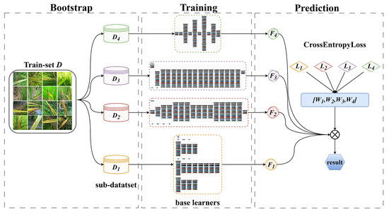
Figure 3.
Depth-guided aggregation algorithm.
2.3.1. Recognition Model Based on Attention Mechanism in Prominent Positions
MobileNetV3-large, ShuffleNetV2-2.0, YOLOv5s-cls, and EfficientNet-B0 are common high-performance convolutional neural networks that have a lighter structure than traditional neural networks. However, they still suffer from performance issues that are easily affected by background noise when identifying rice diseases in complex field backgrounds. Therefore, this study introduces the salient positions-based attention (SPA) mechanism into the lower and middle layers of MobileNetV3-large, ShuffleNetV2-2.0, YOLOv5s-cls, and EfficientNet-B0 to improve the network model and enhance its recognition performance.
- (1)
- Attention Mechanism Based on Salient Location
The salient positions-based attention mechanism (SPA) selects a limited number of salient points in the attention map, and then uses the results of the salient positions selection algorithm to calculate the attention map and aggregate the context information in the channel dimension. This reduces computational complexity while extracting useful contextual information. Figure 4 illustrates the architecture diagram of the SPA attention mechanism.
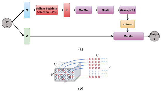
Figure 4.
Attention mechanism based on saliency. (a) SPA attention mechanism architecture, (b) SPS algorithm.
The following equations describe the attention mechanism based on the saliency attention mechanism:
where, is the input and output feature maps; and are the query and key matrices generated by the transformations and ; is the saliency matrix generated by the salient location selection algorithm; is the affinity matrix; is the number of spatial locations of the feature maps ; and is the number of channels. The feature map is transformed by two linear transformations to form the query and value matrices. The matrix is passed to the salient positions selection (SPS) algorithm. The output matrix of the SPS module is the matrix of the first salient positions in the matrix. Figure 4b illustrates the selection process, in particular the dimensionality change. The affinity matrix is calculated using the selected data from the first positions. After the softmax operation is performed on the affinity matrix along the channel dimensions during the aggregation process, the value matrix is multiplied with the affinity matrix and reshaped to to obtain the output feature map .
- (2)
- Salient Positions Selection (SPS)
The salient positions selection (SPS) algorithm plays an important role in the proposed salient position-based attention mechanism (SPA). Salient position selection for global context information will reduce the complexity of the self-attention mechanism computation, and, more importantly, extracts positive context information when modeling global dependencies. The pseudo-code of the proposed SPS algorithm is shown in Algorithm 1: Pseudo-code for prominent position selection algorithm.
| Algorithm 1: Salient Positions Selection (SPS) Algorithm |
| Input: a matrix of size , a hyperparameter ; |
| Output: a matrix of size ; |
| 1. Calculate the square of along the channel dimension; |
| 2. Sum along the channel dimension to get ; |
| 3. Select the largest location from and record it as index ; |
| 4. Return matrix |
Since the histogram of the feature map data for all channels roughly follows a Gaussian distribution, it is valid to choose the square of the data as the importance metric. To emphasize the locations with higher activation values in the feature map, the square matrix is computed along the channel dimension for the transpose of the input query matrix. Summing the resulting squared matrix along the channel dimension yields , which combines the activation strengths of each location across all channels into a single value, resulting in an overall significance measure for each location. The largest values from are selected, the most important salient locations in the feature map, which reduces the amount of data to be processed by selecting the salient locations and thus reduces the computational complexity. Finally, based on the index of the selected salient locations, the features corresponding to these locations are extracted from the original query matrix to form the output matrix for subsequent attention computation in place of the attention mechanism of the full feature map, which further reduces the computational effort.
2.3.2. DL-Bagging Algorithm
The Deep Bootstrap Aggregating (DB) algorithm is constructed by combining the bagging algorithm with a deep learning model. The algorithm is divided into two phases: the first phase is the dataset sampling and base learner training based on the Deep Bootstrap Aggregating (DB) algorithm and the second phase is the integration of base learner predictions based on a simple voting strategy.
The Deep Bootstrap Aggregating algorithm mainly adopts the Bootstrap sampling to realize the production of datasets with the same underlying distribution and feature information, but are not identical, which enhances the diversity and comprehensiveness of model feature extraction. The main advantages of this method are as follows:
- Significantly reduces model variance and improves model stability by using multiple mutually independent base learners.
- Parallel computing speeds up model training.
- Multiple sub-datasets are generated by random sampling to avoid overfitting of the model to the training data.
Among them, Bootstrap is a sampling method with put-back, which achieves the goal of building an adequate sample set using a limited number of samples after many repeated samplings by using a resampling technique, i.e., randomly selecting a given number of samples from the original sample and generating a new set of samples that are the same size as the original sample, but with a different distribution [28].
The training set is sampled using Bootstrap, and multiple samples are taken to obtain training subsets , and the training subset is of the same size as the training set . For each base learner, use a different training subset for training to get base learners , then use these base learners to predict the target object separately to get predicted probability distributions , which are used as inputs to the phase II of the Deep Bootstrap Aggregating algorithm.
- (1)
- The first stage
In the first phase of this study, the main task is to construct a base model based on the depth-guided aggregation algorithm. The core of this phase is to utilize the bootstrap sampling technique to generate multiple sub-datasets with the same underlying distribution but not identical feature information from the original training set. In this way, the diversity and comprehensiveness of the model’s feature extraction can be significantly improved, while reducing the variance of the model and improving its stability, and also accelerating the speed of model training due to the possibility of parallel computing.
In the specific implementation process, bootstrap sampling is first performed on the training set to generate multiple subsets of the same size as the original training set but with different distributions. Then, a base learner is trained separately for each subset, and finally, multiple base learners are obtained. These base learners are structurally independent of each other and can extract feature information from different perspectives because they use different training subsets for training, thus effectively avoiding overfitting of the model to the training data. During the training process, techniques such as the Adam optimizer, cross-entropy loss function, and cosine annealing learning rate scheduler are used to ensure efficient training and performance optimization of the model. The pseudo-code of the first stage of the Deep Bootstrap Aggregating algorithm is shown in Algorithm 2: Pseudo-code for the depth-guided aggregation algorithm (stage 1).
| Algorithm 2: Deep Bootstrap Aggregating Algorithm (Stage 1) |
| Input: training set . |
| The training parameters , the |
| Output: base learner . |
| Begin |
| Initialize Loss_function, Optimizer, Scheduler |
| Bootstrap N samples |
| For do |
| For do |
| For inputs in batch_size do |
| Forward(inputs) |
| Loss_function.CrossEntryLoss(label_smooting) |
| Backward(loss) |
| Optimizer. |
| Scheduler.CosineAnnealingLR |
| Return |
| End |
- (2)
- The second stage
In the second phase of this research, the main task is to construct an integrated model based on a Deep Bootstrap Aggregating algorithm. The machine learning-based recognition algorithm has two types of outputs: category-labeled outputs and predicted probability outputs for each category, which correspond to Majority/Hard Voting (Majority/Hard Voting, HV) [29] and Soft Voting (Soft Voting, SV) [30], respectively. The second stage of the Deep Bootstrap Aggregating algorithm uses hard voting, i.e., by counting the votes of the output categories recognized by the base learner for the target objects, the category with the most votes is the prediction. Assuming that there are categories of target candidates, the set of category labels of target candidates is , there are classifiers , and for the prediction samples or can be recorded. The statistics of prediction results are shown in Table 2.
Table 2.
Tabulation of hard ballots.
Each classifier has one chance to vote for the category label of the predicted sample among the candidate classes and the result of the voting can be expressed as Equation (4):
As can be seen from Table 2, each row in the table is a unique 1 vector, when a classifier gives a vote to a candidate class , its corresponding ballot is recorded as 1. Observing from the column direction, the column is the vote obtained by the candidate class , and the last row indicates the obtained result of each candidate class, and the candidate class that obtains the most votes is the final prediction result. The final decision result of the classifier on the predicted sample is denoted as , and the calculation process can be expressed as Equation (5):
2.3.3. An Improved Depth-Guided Aggregation Algorithm Based on Cross-Entropy Loss
The simple voting strategy utilized in stage 2 of the Deep Bootstrap Aggregating algorithm only focuses on the category labels but ignores the probabilistic information predicted by the model, which may be subject to the role of low-accuracy models and generate randomness in the case of a tie vote, increasing the uncertainty of the results. In order to be able to enhance the integration effect of the Deep Bootstrap Aggregating algorithm, this study designs the Cross-Entropy Loss-Based Weighted Voting Strategy (Cross-Entropy Weighted Soft Voting, CEWSV) based on the soft voting method. For a detailed description of the cross-entropy loss function, see Appendix A.
In the traditional soft voting approach, the prediction probabilities of all base learners are considered with equal weight. However, CEWSV assigns a global weight to each base learner’s prediction associated with its performance by virtue of the introduction of the cross-entropy loss value as a weighting metric, where each base learner outputs a probability distribution for each labeled sample and the cross-entropy loss measures the difference between these probability distributions and the true label. The cross-entropy loss measures the difference between these probability distributions and the true labels, and the global weights are computed with the help of the performance of the integration model on a large number of labeled samples. A lower cross-entropy loss means that the base-learner’s predictions are closer to the true labels, and should have a greater say in the final integration decision.
Weighted voting strategy based on cross-entropy loss
Hard voting is a binary voting mechanism where classifiers must make an explicit choice, i.e., they can only choose between “agreeing” or “disagreeing” with a candidate. Soft voting, also known as proportional voting, is a voting method that allows voters to express their support for different candidates, and the classifier can split the votes with a value of 1 to different candidates based on its own preference, and then Equation (4) becomes a probabilistic expression, as shown in Equation (6):
Soft voting can be viewed as a weighted average fusion of base learners using the same weighting parameters, while weighted voting assigns different weighting parameters to different base learners. The method reduces the effect of high bias of some base learners by rewarding the base learners with good performance and penalizing the base learners with poor performance. In this study, the cross-entropy loss (CEL) value with label smoothing is used as a reference for weight assignment. The loss value is first calculated to quantify the degree of difference between the predicted and actual results of the base learners, i.e., the prediction error, as shown in Equation (7):
where denotes the number of categories; is a hyperparameter for label smoothing; denotes an indicator function, i.e., if the true label of the predicted object is equal to the result predicted by the model, the value of this function is 1, otherwise it is 0; and denotes the output value of the neural network.
In order to obtain a set of weight parameters applicable globally, the average cross-entropy loss values of the base learners over all labelled samples are first calculated to obtain a vector of loss values . In order to ensure that a small loss value does not effectively reward a high-performing model, a power function is used to amplify the loss value to , in order to enhance the relative disparity between different base learners. Since a larger loss value indicates a worse prediction performance of the corresponding learner, the inverse of the amplified loss value is taken as , and in order to ensure that the sum of the weight parameters is 1, normalization is performed to obtain a set of global weight parameters, and the computation process is shown in Equation (8):
When predicting the target object , the global weight parameter is assigned to the prediction probability distribution output by the corresponding base learner, and the contribution of different learners to the final prediction result is adjusted to obtain the weighted prediction probability distribution, as shown in Equations (9) and (10):
where is the weight parameter assigned to the base learner; is the probability of the base learner to predict the target object for the category; the probability distribution after model integration is obtained by accumulating along the column vector direction ; and the category label corresponding to the maximum probability value is the final prediction result. The final decision result of the classifier on the predicted sample is denoted as , and the computation process can be expressed as Equations (11) and (12):
2.4. Evaluation Metrics
In this study, accuracy (Acc), precision (P), recall (R), F1-core (F1), parameter count (Param, P), and computational effort (FLOPs, F) were used to comprehensively measure the performance of the network model on rice disease recognition [31]. Assuming that a certain type of disease is positive and the rest of the diseases are negative, TP denotes the number of samples in which the actual positive category is correctly determined as positive; FP denotes the number of samples in which the actual negative category is incorrectly determined as positive; FN denotes the number of samples in which the actual positive category is incorrectly determined as negative; and TN denotes the number of samples in which the actual negative category is correctly determined as the corresponding negative category. Accuracy is the most commonly used performance metric and is defined as the ratio of correct predictions to total predictions; the higher the value, the better the performance of the model, calculated as shown in Equation (13):
In order to observe whether the model misclassifies or not, precision is used as a further measure. Precision, also known as check accuracy, indicates the proportion of samples identified by the model as being in the positive category that are in the correct category. This value focuses on the number of samples statistically predicted to be in the positive category that are correct, and is calculated as shown in Equation (14):
In order to observe whether the model misses a judgment or not, the recall rate is used as a measure. The recall rate, also known as the check-all rate, indicates the proportion of samples recognized by the model as positive class in the actual positive class samples, and this value measures the ability of the model to recognize all positive class samples, calculated as shown in Equation (15):
However, precision and recall are a pair of contradictory indicators. Model recognition requires that the higher the threshold, the higher the precision and lower the recall, and the lower the threshold, the lower the precision and higher the recall. In order to synthesize the proposed score, which is a kind of weighted average of precision and recall, in the merging process, the weight of recall is times of the precision. The computation is shown in Equation (16):
When precision and recall are equally important, i.e., , then it is the F1 score, which is defined as the reconciled average of precision and recall, calculated as shown in Equation (17):
For the multi-class recognition problem, the accuracy measure is the global sample prediction, and the precision, recall, and F1 score are the evaluation metrics for individual classes, so this paper adopts the macro-average (macro-averaging) method for these three evaluation metrics averaged over each class to evaluate the global prediction performance of the model. The calculation of average precision , average recall , and average F1 score [32] is shown in Equation (18):
The number of parameters, which is the core metric for evaluating the measure of algorithmic complexity, grows positively correlated with the increase in hardware configuration requirements of the computational graph, which is defined [33] as shown in Equation (19):
where , , and denote the number of parameters in the convolutional layer, fully connected layer, and network model, respectively; denotes the size of the convolutional kernel; denotes the number of input feature map channels; denotes the number of output feature map channels; and and denote the number of input and output weights in the fully connected layer, respectively.
In addition, when evaluating the computing efficacy of the algorithmic architecture, the experiments use floating-point arithmetic as a metric to reflect the difference in the computational complexity of the various types of network models, where a higher value implies that the model inference process consumes more processor computation cycles, which is defined [34] as shown in Equation (20):
where , , and denote the computational complexity of the convolutional layer, fully connected layer and network model; and and denote the scale size of the output feature map.
3. Experimental Results
3.1. Selection and Comparison of Base Learners
In this experiment, four base models were trained, optimized, and tested separately using the rice leaf disease dataset. First, we explored the performance of five different depth and width models of YOLOv5-cls on the rice leaf disease dataset. These five versions of the model were trained and tested separately and evaluated in terms of four aspects: number of model parameters, model complexity, recognition accuracy, and FPS, and the results are shown in Table 3.
Table 3.
Comparison of results from five versions of YOLOv5-cls on rice leaf disease validation set.
As can be seen from Table 3, YOLOv5s-cls has the highest recognition accuracy on the rice leaf disease dataset, and its number of parameters and complexity satisfy the lightweight requirement. Compared with the lightest YOLOv5n-cls, YOLOv5s-cls better balances the model recognition performance while reducing the training cost and increasing the inference speed. Therefore, YOLOv5s-cls is used for subsequent experiments.
Next, YOLOv5s-cls, EfficientNet-B0, MobileNetV3, and ShuffleNetV2 are trained without label smoothing and learning rate optimization strategies, respectively, keeping other hyperparameters consistent. Subsequently, the label smoothing and cosine annealing learning rate optimization strategies are added to train the four base learners again. The training results before and after optimization are shown in Figure 5.
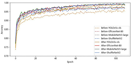
Figure 5.
Results of single models before and after optimization on rice leaf disease validation set.
As can be seen from Figure 5, the optimized model is more stable, with accuracy gradually increasing and eventually leveling off as the epoch increases, indicating that the model is better trained. The final accuracies of YOLOv5s-cls, EfficientNet-B0, MobileNetV3, and ShuffleNetV2 on the rice leaf disease dataset are, respectively, 98.42%, 99.05%, 98.72%, and 99.02%. Finally, the four base models were tested to calculate the recognition accuracy, macro precision, macro recall, and macro F1 score, and the results are shown in Table 4. These four lightweight networks save training resources, and all of them have high recognition accuracy with small performance differences, so they are selected as the base learners for integrated learning.
Table 4.
Comparison of results from base learners.
3.2. Test Platform and Parameter Settings
The computer used in this study is a Lenovo Legion Y7000 made in China, equipped with an Intel(R) Core (TM) i7-12700H CPU, 2.70 GHz, 64.0 GB RAM, and an NVIDIA GeForce RTX 3060 graphics card; CUDA version 11.6; Cudnn version 8.3.2; and Windows 11 64-bit operating system. The software used mainly includes OpenCV image processing software and Pytorch 1.13 Python 3.10 deep learning framework, and the program was compiled using the Python language.
First, we conducted a series of ablation experiments to evaluate the effectiveness of the method in order to determine the hyperparameters that are better for the model training results. The final hyperparameter settings are shown in Table 5.
Table 5.
Training parameter configuration.
3.3. Comparison of the Performance of Adding SPA at Different Stages
In order to verify the performance enhancement of the improved SPA-M, SPA-S, SPA-Y, and SPA-E network models for rice disease recognition, the unity of the structure and initial parameter configuration of each network model was strictly maintained during this experiment, and the hyperparameter of the salient position-based attention mechanism SPA was set to 2. The improved SPA-M, SPA-S, SPA-Y, and SPA-E network models were compared with their original network models. The improved SPA-M, SPA-S, SPA-Y, and SPA-E network models are compared with their original network models, and the results of the parameter counts, computation, and recognition performance comparison of each network model are shown in Table 6 and Table 7.
Table 6.
Network model parametric quantities and calculations.
Table 7.
Comparison of network model performance.
Comparing the experimental results in Table 6 and Table 7, compared to the original base networks MobileNetV3-large, ShuffleNetV2-2.0, YOLOv5s-cls, and EfficientNet-B0, the improved SPA-M, SPA-S, SPA-Y, and SPA-E have an increase in the number of parameters by up to 0.002 M, 2.863 M, 0.05 M, and 0.005 M, and the computational volume increased by up to 0.009 G, 0.108 G, 0.024 G, and 0.034 G. The improved network models increased the recognition accuracy of rice diseases by up to 1.191%, 0.357%, 0.952%, and 1.191%; the average accuracies increased by 1.102%, 0.441%, 0.970%, and 1.088%; average recall improved by 1.191%, 0.357%, 0.952%, and 1.191%; and average F1 score values improved by 1.169%, 0.370%, 0.956%, and 1.193%. By introducing a salient position-based attention module to optimize the feature selection mechanism, the improved algorithm has significantly improved the recognition of rice diseases while maintaining the computational efficiency, and compared to the base model, this improvement presents a better performance in all the evaluation metrics and achieves a breakthrough in performance at the cost of only a small amount of resource consumption.
Moreover, to balance the performance and efficiency of the network model and determine a value that ensures the model can effectively process information while maintaining high operational efficiency, this experiment was conducted with settings of two, four, and eight, respectively, and comparative experiments were carried out on SPA-M, SPA-S, SPA-Y, and SPA-E. Transfer learning technology was used to initialize the weight parameters of each network model, and the training of the rice disease dataset was ultimately completed. The recognition accuracy rates of various network models under different settings are compared in Table A1. A detailed comparison of recognition accuracy rates for various network models using different K values is provided in Appendix B.
3.4. DL-Bagging Based Model for Combining Different Base Learners
The performance of integrated learning models with different combinations of base learners is explored in the experiments. Random combinations of YOLOv5s-cls, EfficientNet-B0, MobileNetV3, and ShuffleNetV2 were fused into a new DL-Bagging based integrated learning model. The training parameters are kept consistent with single model training. The recognition accuracy, macro-accuracy, macro-recall, macro-F1 score, and the mean value of each evaluation index of the integrated learning model with different base-learner combinations for rice leaf diseases are shown in Table 8, where M denotes MobileNetV3, S denotes ShuffleNetV2, Y denotes YOLOv5s-cls, and E denotes EfficientNet-B0.
Table 8.
Performance of different integration models.
As can be seen from Table 8, the integrated models have a high level of recognition performance, where the MS, ME, SE, YE, MSE, SYE, and MSYE models have higher recognition performance compared to each base model in their combination, with the highest recognition accuracy, average precision, average recall, and average F1 scores of 98.095%, 98.205%, 98.095%, and 98.108%, which are 0.238%, 0.229%, 0.238%, and 0.246% higher than the best performing single model SPA-Y.
In order to verify the performance enhancement of the depth-guided aggregation algorithm by CEWSV, a weighted voting strategy based on the cross-entropy loss improvement, the same combination of models as described above is used for testing on the rice disease dataset. The recognition accuracy of the models on the test set is shown in Table 9, where HV denotes hard voting, SV denotes soft voting, and CEWSV denotes a weighted voting strategy based on cross-entropy loss.
Table 9.
Comparison of different integration strategies.
As can be seen from Table 9, the recognition accuracy of MS, SY, MSY, MSE, and MYE network models is improved when soft voting is used as the integration strategy compared to the hard voting method, in which the recognition accuracy is improved by up to 0.238%, and the recognition accuracy of the MY, ME, and SYE models is kept unchanged when using the improved CEWSV based on soft voting as the integration strategy, and the remaining network models of the network models are improved, with the highest improvement of 0.476%, among which the MSE and MSYE network models have the highest recognition accuracy of 98.333%, which is improved by 0.238% compared to the original integration strategy HV. To further observe the performance of the integrated models, the accuracy, average precision, average recall, and average F1 score of the integrated models for recognition on the rice disease test set were compared, as shown in Table 10.
Table 10.
Performance comparison of integrated models.
The average precision improved by up to 0.439%, the average recall by up to 0.476%, and the average F1 score by up to 0.47%. The MSE and MSYE network models had the best performance in each of the evaluation metrics, with recognition accuracy, precision, recall, and F1 scores of 98.333%, 98.412%, 98.333%, and 98.343%. Compared to the single base learners SPA-M, SPA-S, SPA-Y, and SPA-E, recognition accuracy is improved by 1.19%, 0.595%, 0.476%, and 0.476%; the average precision is improved by 1.24%, 0.625%, 0.436%, and 0.458%; the average recall is improved by 1.19%, 0.595%, 0.476%, and 0.476%; and the average F1 score improved by 1.204%, 0.604%, 0.481%, and 0.475. In order to reduce the cost of deployment at the edge end, the MSE integration model was chosen as the final model for subsequent deployment.
3.5. Comparison with Other Mainstream Models
To further validate the recognition performance of the model proposed in this paper, other mainstream convolutional neural networks are trained and tested on the rice disease dataset using the same experimental setup as described above. In this paper, ResNet50, DenseNet121, and ConvNeXt-tiny are selected to be compared with the best integrated model MSE, and the recognition accuracies, average precision on the rice disease test set, average recall, and average F1 score are shown in Figure 6.
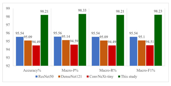
Figure 6.
Comparison of other mainstream models.
As can be seen in Figure 6, the MSE integrated model proposed in this paper exhibits excellent performance on all evaluation metrics, with a recognition accuracy of 98.333% on the test set, compared to 96.429% for ResNet50, 96.905% for DenseNet121, and 95.952% for ConvNeXt-tiny. The MSE model performance in the rice disease identification task. The recognition performance of the MSE model proposed in this paper on the rice disease dataset is fully validated through comparison experiments with mainstream CNN models such as ResNet50, DenseNet121, and ConvNeXt-tiny.
To further analyze the model’s recognition performance for each disease category, a confusion matrix (also known as a probability matrix) is used to visualize the model’s recognition results. Each column in the confusion matrix represents the category predicted by the model, and the sum of the columns indicates the number of samples predicted to belong to that category. Each row represents the true category of the data, and the sum of the rows indicates the number of true samples in that category, as shown in Figure 7. ResNet50, DenseNet121, ConvNeXt-tiny, and MSE performed identically on the tungro and healthy categories, achieving an accuracy rate of 100%. ResNet50, DenseNet121, and ConvNeXt-tiny also performed identically on the bacterial leaf blight, with an accuracy rate of 94.048%. The MSE ensemble model shows a significant improvement in recognition performance, with an accuracy rate of 97.024%. The recognition accuracy rates for rice blast disease using ResNet50, DenseNet121, ConvNeXt-tiny, and MSE are 92.262%, 93.452%, 90.476%, and 95.238%, respectively. The identification accuracy rates of ResNet50, DenseNet121, ConvNeXt-tiny, and MSE for brown spot disease are 95.833%, 97.024%, 95.238%, and 99.405%, respectively. The MSE ensemble model proposed in this paper outperforms mainstream models across all categories, demonstrating superior identification performance.
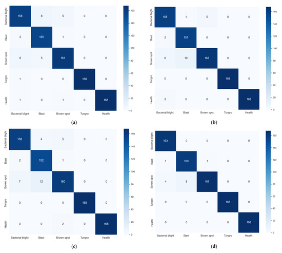
Figure 7.
The confusion matrix of other models and our model. (a) ResNet50, (b) DenseNet121, (c) ConvNeXt-tiny, (d) MSE.
4. Discussion
Recent studies on rice disease classification have made significant progress using deep learning techniques, particularly with lightweight models and ensemble methods. For instance, Gan et al. [35] proposed that BiFPN multi-scale fusion combined with the Wise-IoU loss function can improve small-sample generalization ability, but the mAP of small samples in natural environments is still 3.8% lower than that in laboratory conditions. Similarly, Wang et al. [36] proposed a stacked ensemble of CG-EfficientNet models, achieving 96.10% accuracy by leveraging attention mechanisms and sequential least squares programming for weight optimization. While this approach demonstrates commendable performance, it primarily focuses on balancing model accuracy and computational efficiency, with limited emphasis on handling complex field conditions or small-sample datasets. Jia et al. [37] proposed the MobileNet-CA-YOLO model, which significantly improved the efficiency and lightweight level of rice pest and disease detection by combining the MobileNetV3 lightweight network, the coordinate attention mechanism (CA), and the SIoU loss function. However, their dataset mainly comes from web crawling, and the sample coverage and diversity may be insufficient. Moreover, it does not include real scene data under complex field environments (such as occlusion and light changes), which affects the generalization ability of the model in practical applications. These methods typically rely on single-model optimizations or simple ensemble strategies, which may not fully exploit the diversity of feature representations or adapt dynamically to varying field conditions.
Our method, CEL-DL-Bagging, addresses these limitations by integrating a salient position attention (SPA) mechanism with a cross-entropy loss-weighted voting strategy, achieving 98.33% accuracy. Unlike previous approaches, our framework combines multiple lightweight models (YOLOv5s-cls, EfficientNet-B0, MobileNetV3, and ShuffleNetV2) through Bootstrap Aggregating (Bagging), enhancing feature diversity and robustness. The SPA mechanism specifically targets diagnostically relevant regions, reducing interference from complex backgrounds, while the adaptive weighting strategy ensures optimal contributions from each base learner. This dual focus on attention and ensemble diversity allows our model to outperform existing methods in both accuracy and generalization, particularly in natural field environments where lighting and occlusion variations are prevalent.
While the proposed CEL-DL-Bagging framework demonstrates superior performance in rice leaf disease identification, several important considerations and limitations merit discussion.
(1) The field rice disease dataset used in this paper was sourced from the rice green high-yield, efficient, and productive demonstration fields in Gaoyou City, and Yangzhou City, both in Jiangsu Province. The experiment utilized network data expansion, data enhancement, and transfer learning techniques to mitigate the impact of limited data volume. Further expansion of the field rice disease dataset will be required with the assistance of agricultural researchers;
(2) The field rice disease recognition model in this paper has not yet been tested with a more diverse range of rice disease phenotypic features. Further efforts are needed to increase data diversity and validate the model’s performance under other disease manifestation scenarios to enhance its generalization capability;
(3) This paper improved the network model’s performance in identifying rice diseases in the field through a position-based attention mechanism and an improved depth-guided aggregation algorithm. However, there is still room for improvement. In the future, we will attempt to integrate more advanced deep learning technologies with the identification model to improve identification accuracy, speed, and adaptability under different environmental conditions, thereby optimizing the rice disease identification model in the field.
5. Conclusions
This study presents the CEL-DL-Bagging framework for accurate rice leaf disease identification in complex field environments. By integrating a salient position attention mechanism with cross-entropy loss-weighted ensemble learning, the method achieves 98.33% accuracy while maintaining computational efficiency for practical deployment. The proposed approach outperforms existing models by effectively combining lightweight network design with adaptive feature extraction and decision fusion. This work provides a robust solution for real-world agricultural applications and demonstrates the potential of attention-based ensemble learning in plant disease recognition. To further demonstrate the superiority and effectiveness of this model, we have successfully deployed it to the edge device Jetson Orin Nano. For details, please refer to the supplementary materials section. Future efforts will focus on expanding the system’s applicability to diverse field conditions and crop varieties.
Supplementary Materials
The following supporting information can be downloaded at: https://www.mdpi.com/article/10.3390/agriengineering7080255/s1, To validate the feasibility of the proposed CEL-DL-Bagging framework in practical applications, we successfully deployed the optimized MSE ensemble model on the Jetson Orin Nano edge device. Due to the limited performance of edge devices compared to PCs, the FPS of the rice disease recognition device based on Jetson Orin Nano is approximately 14–15, but its recognition speed still meets real-time requirements. Furthermore, we designed a rice disease recognition client system using the PyQT5 framework, which allows users to either upload local videos or enable the camera for online or real-time rice disease recognition. Finally, to meet the needs of agricultural researchers for portable rice disease identification in field scenarios, we also used the Bambu Lab P1S series 3D printer from Tuozhu for housing fabrication. The physical design and fabrication of the field rice disease identification device were ultimately completed. The specific display pictures have been included in the Supplementary Materials. Figure S1. Real-time recognition effect display at the edge end; Figure S2. Rice Identification System Client Display; Figure S3. 3D printed model of a rice disease identification device for use in the field; Figure S4. Field Rice Disease Identification Instrument.
Author Contributions
Conceptualization, Z.Z., R.W. and S.H.; methodology, R.W.; software, R.W.; validation, Z.Z., R.W. and S.H.; formal analysis, R.W.; investigation, R.W.; resources, R.W. and S.H.; data curation, R.W. and S.H.; writing—original draft preparation, R.W.; writing—review and editing, Z.Z.; visualization, Z.Z.; supervision, Z.Z.; project administration, Z.Z.; funding acquisition, Z.Z. All authors have read and agreed to the published version of the manuscript.
Funding
This research was funded by the Jiangsu Province Graduate Practical and Innovation Program (SJCX25_2296).
Institutional Review Board Statement
Not applicable.
Informed Consent Statement
Not applicable.
Data Availability Statement
The data that support the findings of this study are available from the corresponding author upon reasonable request.
Conflicts of Interest
The authors declare that they have no conflicts of interest to report regarding the present study.
Appendix A
Cross-Entropy Loss Function
The softmax function is commonly used to calculate the predicted probability distribution of each category in the category recognition task, which maps a set of output values of the neural network into a predicted probability distribution , and the calculation process is shown in Equation (A1). In this study, the Cross-Entropy Loss [38] function is used as a loss function to calculate the loss value to quantify the degree of difference between the predicted label and the true label probability, as shown in Equation (A2):
where denotes the true label of the predicted object; denotes the label predicted by the model; and denotes the probability distribution of the true label, i.e., when the model predicts accurately, then it is 1, and vice versa, it is 0. At this point, the cross-entropy loss only takes into account the loss of the position of the true label and ignores the loss of the position of the other labels, so that the model is overly concerned about increasing the probability of predicting the correct label rather than focusing on decreasing the probability of predicting the incorrect label.
In image recognition tasks, training samples usually have a small number of mislabels in order to avoid over-reliance on the labels of the training samples. When the objective function is cross-entropy, a label smoothing regularization method is used to prevent the model from overfitting and calibration errors. This method softens the labels by adding noise to the true label probability distribution, reduces the weight of the categories of the true labels in the calculation of the loss function, and finally achieves the effect of suppressing overfitting. Adding label smoothing changes the true label probability distribution in Equation (A2), given by Equation (A3), where is a smaller hyperparameter [39]. The cross-entropy loss function is also changed, as shown in Equation (A4):
Appendix B
Comparison of the Effects of Hyperparameter K
In the salient position selection algorithm, adjusting hyperparameters controls the scale of the selected salient positions in the query matrix. Smaller values reduce computational complexity and memory usage, making them suitable for real-time applications and resource-constrained devices, but may result in the loss of critical information and affect model performance. Larger values can capture more contextual information, potentially improve accuracy, but increase computational load and memory requirements, and may even lead to overfitting. As shown in Table A1, using a saliency attention mechanism to improve the network model only causes a slight decrease in model performance in a few cases. When the insertion position is the second layer, the accuracy of SPA-M is 97.143%, showing the greatest improvement compared to the original MobileNetV3-large network model, with an increase of 1.119%. When the insertion position is the second layer, the accuracy of SPA-S is 97.738%, showing the greatest improvement compared to the ShuffleNetV2-2.0 network model, with an increase of 0.833%. When the insertion position is the third layer, the accuracy of SPA-Y is 97.857%, which is the highest improvement compared to the original YOLOv5s-cls network model, with an increase of 0.952%. When the insertion position is the fourth layer, the accuracy of SPA-E is 97.857%, which is the highest improvement compared to the EfficientNet-B0 network model, with an increase of 1.667%.
Table A1.
Network model accuracy at different k values.
Table A1.
Network model accuracy at different k values.
| Model | Layer | /% | ||
|---|---|---|---|---|
| k = 2 | k = 4 | k = 8 | ||
| SPA-M | (1,0,0,0) | 96.190 (+0.238) | 96.548 (+0.596) | 96.548 (+0.596) |
| (0,1,0,0) | 97.143 (+1.191) | 95.714 (−0.238) | 96.905 (+0.953) | |
| (0,0,1,0) | 95.833 (−0.119) | 96.190 (+0.238) | 96.429 (+0.477) | |
| (0,0,0,1) | 96.071 (+0.119) | 95.952 (+0.000) | 95.952 (+0.000) | |
| SPA-S | (1,0,0,0) | 97.024 (+0.119) | 97.619 (+0.714) | 97.262 (+0.357) |
| (0,1,0,0) | 97.262 (+0.357) | 96.667 (−0.238) | 97.738 (+0.833) | |
| (0,0,1,0) | 97.262 (+0.357) | 96.786 (−0.119) | 97.024 (+0.119) | |
| (0,0,0,1) | 97.024 (+0.119) | 96.905 (+0.000) | 97.262 (+0.357) | |
| SPA-Y | (1,0,0,0) | 97.143 (+0.238) | 96.905 (+0.000) | 97.262 (+0.357) |
| (0,1,0,0) | 97.500 (+0.595) | 97.143 (+0.238) | 97.500 (+0.595) | |
| (0,0,1,0) | 97.857 (+0.952) | 97.381 (+0.476) | 97.143 (+0.238) | |
| (0,0,0,1) | 97.619 (+0.714) | 97.381 (+0.476) | 97.381 (+0.476) | |
| SPA-E | (1,0,0,0) | 97.381 (+1.191) | 96.429 (+0.239) | 97.262 (+1.072) |
| (0,1,0,0) | 96.548 (+0.358) | 96.190 (+0.000) | 96.548 (+0.358) | |
| (0,0,1,0) | 96.310 (+0.120) | 97.262 (+1.072) | 96.429 (+0.239) | |
| (0,0,0,1) | 96.190 (+0.000) | 97.857 (+1.667) | 96.667 (+0.477) | |
References
- Tardieu, F.; Cabrera-Bosquet, L.; Pridmore, T.; Bennett, M. Plant phenomics, from sensors to knowledge. Curr. Biol. 2019, 27, R770–R783. [Google Scholar] [CrossRef]
- Li, L.; Zhang, Q.; Huang, D. A review of imaging techniques for plant phenotyping. Sensors 2014, 14, 20078–20111. [Google Scholar] [CrossRef] [PubMed]
- Wang, Y.; Wang, H.; Peng, Z. Rice diseases detection and classification using attention based neural network and bayesian optimization. Expert Syst. Appl. 2021, 178, 114770. [Google Scholar] [CrossRef]
- Phadikar, S.; Sil, J.; Das, A.K. Rice diseases classification using feature selection and rule generation techniques. Comput. Electron. Agric. 2013, 90, 76–85. [Google Scholar] [CrossRef]
- Lu, Y.; Yi, S.; Zeng, N.; Liu, Y.; Zhang, Y. Identification of rice diseases using deep convolutional neural networks. Neurocomputing 2017, 267, 378–384. [Google Scholar] [CrossRef]
- Jiang, F.; Lu, Y.; Chen, Y.; Cai, D.; Li, G. Image recognition of four rice leaf diseases based on deep learning and support vector machine. Comput. Electron. Agric. 2020, 179, 105824. [Google Scholar] [CrossRef]
- Hu, K.; Liu, Y.; Nie, W.; Zheng, X.; Zhang, W.; Liu, Y.; Xie, T. Rice pest identification based on multi-scale double-branch gan-resnet. Front. Plant Sci. 2023, 14, 1167121. [Google Scholar] [CrossRef]
- Cai, J.; Pan, R.; Lin, J.; Liu, J.; Zhang, L.; Wen, X.; Chen, X.; Zhang, X. Improved EfficientNet for corn disease identification. Front. Plant Sci. 2023, 14, 1224385. [Google Scholar] [CrossRef]
- Butera, L.; Ferrante, A.; Jermini, M.; Liu, J.; Zhang, L.; Wen, X.; Chen, X.; Zhang, X. Precise agriculture: Effective deep learning strategies to detect pest insects. IEEE/CAA J. Autom. Sin. 2021, 9, 246–258. [Google Scholar] [CrossRef]
- Zhou, H.; Chen, J.; Niu, X.; Da, Z.; Qin, L.; Ma, L.; Li, J.; Su, Y.; Qi, W. Identification of leaf diseases in field crops based on improved ShuffleNetV2. Front. Plant Sci. 2024, 15, 1342123. [Google Scholar] [CrossRef]
- Jocher, G.; Chaurasia, A.; Stoken, A.; Borovec, J.; Kwon, Y.; Michael, K.; Fang, J.; Wong, C.; Yifu, Z.; Montes, D. Ultralytics/yolov5: v6. 2-yolov5 Classification Models, Apple m1, Reproducibility, Clearml and Deci. ai Integrations; Zenodo: Geneva, Switzerland, 2022. [Google Scholar] [CrossRef]
- Yang, X.; Bist, R.; Subedi, S.; Wu, Z.; Liu, T.; Chai, L. An automatic classifier for monitoring applied behaviors of cage-free laying hens with deep learning. Eng. Appl. Artif. Intell. 2023, 123, 106377. [Google Scholar] [CrossRef]
- Zhuang, F.; Qi, Z.; Duan, K.; Xi, D.; Zhu, Y.; Zhu, H.; Xiong, H.; He, Q. A Comprehensive Survey on Transfer Learning. Proc. IEEE 2021, 109, 43–76. [Google Scholar] [CrossRef]
- Hassan, S.M.; Maji, A.K.; Jasinski, M.; Leonowicz, Z.; Jasińska, E. Identification of Plant-Leaf Diseases Using CNN and Transfer-Learning Approach. Electronics 2021, 10, 1388. [Google Scholar] [CrossRef]
- Zhao, H.; Jia, J.; Koltun, V. Exploring self-attention for image recognition. In Proceedings of the IEEE/CVF Conference on Computer Vision and Pattern Recognition, Seattle, WA, USA, 13–19 June 2020; pp. 10076–10085. [Google Scholar]
- Chen, J.; Chen, J.; Zhang, D.; Sun, Y.; Nanehkaran, Y.A. Using deep transfer learning for image-based plant disease identification. Comput. Electron. Agric. 2020, 173, 105393. [Google Scholar] [CrossRef]
- Wang, C.Y.; Liao, H.Y.M.; Wu, Y.H.; Chen, P.-Y.; Hsieh, J.-W.; Yeh, I.-H. CSPNet: A new backbone that can enhance learning capability of CNN. In Proceedings of the IEEE/CVF Conference on Computer Vision and Pattern Recognition Workshops, Seattle, WA, USA, 14–19 June 2020; pp. 1571–1580. [Google Scholar]
- Yuan, P.; Xia, Y.; Tian, Y.; Xu, H. Trip: A transfer learning based rice disease phenotype recognition platform using senet and microservices. Front. Plant Sci. 2024, 14, 1255015. [Google Scholar] [CrossRef] [PubMed]
- Li, X.; Xiao, S.; Zhang, F.; Huang, J.; Xie, Z.; Kong, X. A fault diagnosis method with AT-ICNN based on a hybrid attention mechanism and improved convolutional layers. Appl. Acoust. 2024, 225, 110191. [Google Scholar] [CrossRef]
- Xu, C.; Ding, J.; Qiao, Y.; Zhang, L. Tomato disease and pest diagnosis method based on the stacking of prescription data. Comput. Electron. Agric. 2022, 197, 106997. [Google Scholar] [CrossRef]
- Mathew, A.; Antony, A.; Mahadeshwar, Y.; Khan, T.; Kulkarni, A. Plant disease detection using glcm feature extractor and voting classiffcation approach. Mater. Today Proc. 2022, 58, 407–415. [Google Scholar] [CrossRef]
- He, Y.; Zhang, G.; Gao, Q. A novel ensemble learning method for crop leaf disease recognition. Front. Plant Sci. 2024, 14, 1280671. [Google Scholar] [CrossRef]
- Palanisamy, S.; Sanjana, N. Corn leaf disease detection using genetic algorithm and weighted voting. In Proceedings of the 2023 2nd International Conference on Advancements in Electrical, Electronics, Comunication, Computing and Automation (ICAECA) (IEEE) 2023, Coimbatore, India, 16–17 June 2023; pp. 1–6. [Google Scholar]
- Yang, L.; Yu, X.; Zhang, S.; Zhang, H.; Xu, S.; Long, H.; Zhu, Y. Stacking-based and improved convolutional neural network: A new approach in rice leaf disease identification. Front. Plant Sci. 2023, 14, 1165940. [Google Scholar] [CrossRef]
- Tan, M.; Le, Q. Efficientnet: Rethinking model scaling for convolutional neural networks. In Proceedings of the International Conference on Machine Learning (PMLR), Long Beach, CA, USA, 9–15 June 2019; pp. 6105–6114. [Google Scholar]
- Howard, A.; Sandler, M.; Chu, G.; Chen, L.C.; Chen, B.; Tan, M.; Chu, G.; Vasudevan, V.; Zhu, Y.; Pang, R.; et al. Searching for mobilenetv3. In Proceedings of the IEEE/CVF International Conference on Computer Vision (IEEE)2019, Seoul, Republic of Korea, 27 October–2 November 2019. [Google Scholar]
- Ma, N.; Zhang, X.; Zheng, H.T.; Sun, J. Shufflenet v2: Practical guidelines for efficient cnn architecture design. In Computer Vision (ECCV); Springer: Berlin/Heidelberg, Germany, 2018; pp. 122–138. [Google Scholar]
- Delgado, R. A semi-hard voting combiner scheme to ensemble multi-class probabilistic classifiers. Appl. Intell. 2022, 52, 3653–3677. [Google Scholar] [CrossRef]
- Verma, R.; Chandra, S. RepuTE: A soft voting ensemble learning framework for reputation-based attack detection in fog-IoT milieu. Eng. Appl. Artif. Intell. 2023, 118, 105670. [Google Scholar] [CrossRef]
- Mao, A.; Mohri, M.; Zhong, Y. Cross-entropy loss functions: Theoretical analysis and applications. In Proceedings of the International Conference on Machine Learning. PMLR, Honolulu, HI, USA, 23–29 July 2023; pp. 23803–23828. [Google Scholar]
- Gowda, T.; You, W.; Lignos, C.; May, J. Macro-average: Rare types are important too. arXiv 2021, arXiv:2104.05700. [Google Scholar]
- Xie, Y.; Zhong, X.; Zhan, J.; Wang, C.; Liu, N.; Li, L.; Zhao, P.; Li, L.; Zhou, G. ECLPOD: An Extremely Compressed Lightweight Model for Pear Object Detection in Smart Agriculture. Agronomy 2023, 13, 1891. [Google Scholar] [CrossRef]
- Sun, X.; Shi, Y. The image recognition of urban greening tree species based on deep learning and CAMP-MKNet model. Urban For. Urban Green. 2023, 85, 127970. [Google Scholar] [CrossRef]
- Zoubir, A.M.; Iskandler, D.R. Bootstrap methods and applications. IEEE Signal Process 2007, 24, 10–19. [Google Scholar] [CrossRef]
- Gan, X.; Cao, S.; Wang, J.; Wang, Y.; Hou, X. YOLOv8-DBW: An Improved YOLOv8-Based Algorithm for Maize Leaf Diseases and Pests Detection. Sensors 2025, 25, 4529. [Google Scholar] [CrossRef]
- Wang, Z.; Wei, Y.; Mu, C.; Zhang, Y.; Qiao, X. Rice Disease Classiffcation Using a Stacked Ensemble of Deep Convolutional Neural Networks. Sustainability 2025, 17, 124. [Google Scholar] [CrossRef]
- Jia, L.; Wang, T.; Chen, Y.; Zang, Y.; Li, X.; Shi, H.; Gao, L. MobileNet-CA-YOLO: An Improved YOLOv7 Based on the MobileNetV3 and Attention Mechanism for Rice Pests and Diseases Detection. Agriculture 2023, 13, 1285. [Google Scholar] [CrossRef]
- Lienen, J.; Hüllermeier, E. From label smoothing to label relaxation. In Proceedings of the AAAI Conference on Artificial Intelligence, Vancouver, BC, Canada, 2–9 February 2021; pp. 8583–8591. [Google Scholar]
- Pan, Y.; Su, Z.; Wang, Y.; Guo, S.; Liu, H.; Li, R.; Wu, Y. Cloud-Edge Collaborative Large Model Services: Challenges and Solutions. IEEE Netw. 2025, 39, 182–191. [Google Scholar] [CrossRef]
Disclaimer/Publisher’s Note: The statements, opinions and data contained in all publications are solely those of the individual author(s) and contributor(s) and not of MDPI and/or the editor(s). MDPI and/or the editor(s) disclaim responsibility for any injury to people or property resulting from any ideas, methods, instructions or products referred to in the content. |
© 2025 by the authors. Licensee MDPI, Basel, Switzerland. This article is an open access article distributed under the terms and conditions of the Creative Commons Attribution (CC BY) license (https://creativecommons.org/licenses/by/4.0/).