Multi-Station Agricultural Machinery Scheduling Based on Spatiotemporal Clustering and Learnable Multi-Objective Evolutionary Algorithm

Abstract

The multi-station agricultural machinery scheduling process mainly involves two key stages: order allocation and path planning. Order allocation methods based solely on spatial distance cannot ensure the continuity of agricultural operations. Multi-objective evolutionary algorithms are sensitive to the initial population quality and local search strategies for path planning, where unreasonable initial solutions or improper local search strategies can affect the diversity of solutions. Therefore, we propose a spatiotemporal allocation algorithm that constructs a spatiotemporal distance function to describe the feasibility of continuous operations and evaluates the spatiotemporal proximity of operation points and stations for clustering allocation. In terms of path planning, we design a learnable multi-objective evolutionary algorithm (LMOEA). First, a hybrid initialization strategy is used to enhance the initial population quality; second, a Q-learning-based local search method is constructed to adaptively adjust the search strategy to reduce ineffective iterations; finally, a dynamically adjusted crowding distance mechanism is introduced to improve the distribution of the solution set. Experimental results show that the spatiotemporal allocation algorithm improves the average cost and satisfaction by 4.09% and 3.28% compared to the spatial method. Compared with INSGA-II, HTSMOGA, and NNITSA algorithms, the LMOEA can obtain solutions of higher quality and greater diversity.

1. Introduction

During the agricultural machinery service process, improper resource allocation, information circulation issues, and insufficient emergency response capabilities during peak periods are common challenges [1]. Agricultural service organizations typically face a large number of dispersed fieldwork tasks, each with different times, locations, and requirements. These tasks have seasonal characteristics, especially during the peak agricultural production period, when the demand for agricultural machinery is high and the time windows are tight, leading to inflexible resource allocation among agricultural machinery stations, resulting in equipment idling or overuse. Additionally, the high dispersion of operation points increases the difficulty of scheduling. Without reasonable routing, unnecessary detours and excessive transfer distances can lead to higher operational costs. Furthermore, mismatches between arrival times and farmers’ preferred time windows may reduce service satisfaction, ultimately weakening the long-term cooperation between farmers and cooperatives. On the other hand, the transmission of work information usually relies on manual operations, and delayed updates lead to a mismatch between machinery supply and farmer demand, causing the service organization to be unable to provide targeted services based on farmer needs.

The task assignment work is generally solved using agricultural machinery scheduling methods. The agricultural machinery scheduling problem refers to the reasonable arrangement of tasks, sequence, and operation time of agricultural machinery under limited resources to ensure efficient and economical operations [2].

In recent years, significant progress has been made in agricultural machinery scheduling models, with research focus gradually shifting from single-machine operation optimization to multi-machine coordination and further evolving towards complex multi-region, multi-depot scheduling problems. Early studies mainly focused on the optimization of single or a small number of machines, laying the theoretical and framework foundation for agricultural machinery scheduling models. Guan et al. [3] proposed a framework to manage mechanical movement sequences and coordination deadlocks. This framework offers methodological support for complex scheduling problems. Edwards et al. [4] constructed a multi-machine coordination scheduling framework from the perspective of operational readiness, enhancing efficiency in multi-location operations through task sequence, condition constraints, and location state linkage. Alaiso et al. [5] proposed an integrated scheduling model for agricultural contracting work by systematically describing tasks, resource replenishment points, and machinery attributes, effectively solving agricultural contracting operation scheduling problems. These studies provided basic modeling ideas for agricultural machinery scheduling but still had limitations in dealing with large-scale, multi-entity coordination scheduling problems.

With the development of mechanization and intelligence, agricultural machinery scheduling problems are gradually moving towards multi-machine collaboration, task optimization, and dynamic adjustment. Mohamed et al. [6] started from the perspective of agricultural machinery selection and scheduling, establishing a scheduling plan that minimizes the total cost of machinery. To address the uncertainty in scheduling, Aguayo et al. [7] proposed a cyclic dynamic rescheduling strategy, adjusting field status and machinery location in real-time. Seyyedhasani et al. [8] solved the real-time scheduling problem from the perspective of multi-point path planning. In terms of multi-machine collaboration, Cao et al. [9] explored the task allocation mechanism for multiple agricultural machines; He et al. [10] proposed a coordinated operation plan for harvesters and transporters for fragmented fields; Han et al. [11] focused on the dynamic collaboration between harvesters and auxiliary transport vehicles, effectively reducing operation waiting time. Agricultural machinery service scheduling research mainly focuses on improving service efficiency and resource utilization. In terms of single-region service, He et al. [12] developed an integer programming model to optimize the scheduling of agricultural machinery on fragmented fields. The model allows multiple harvesters to harvest the same field, improving efficiency and shortening the harvest cycle. Si et al. [13] proposed a hierarchical game method to optimize the real-time scheduling of harvesters, enhancing the matching degree of farmer demand and machinery utilization. Hou et al. [14] constructed a service quality evaluation model, considering factors such as time urgency, working conditions, field size, and distance, and adjusted the weight of time urgency dynamically to optimize the agricultural machinery rental plan. However, the single-region service model is often limited by resource capacity and geographical range when facing large-scale operation demands. Ding et al. [15] addressed the underutilization of individual agricultural machinery resources and the lack of trust among all parties involved in scheduling, proposing a blockchain-based regional agricultural machinery resource scheduling system and agricultural machinery scheduling optimization model to reduce regional agricultural production costs and improve resource utilization. However, the single-region service model often faces limitations in terms of resource capacity and geographical range when facing large-scale operation demands.

To address these challenges, multi-regional cooperative scheduling has gradually become a research hotspot. Ma et al. [16] proposed a multi-region coordination architecture to improve the allocation of agricultural machinery resources between regions using an improved knapsack model and hybrid algorithms to solve the resource imbalance problem between regions. Huang et al. [17] proposed a multi-station, multi-machine collaborative real-time response dispatch system based on fuzzy membership degrees to optimize scheduling efficiency and improve farmer satisfaction. Cao et al. [18] established a bi-objective optimization model for wheat harvesting scenarios across regions, providing decision support for multi-regional interconnection scheduling.

In terms of algorithms, with the increase in resource constraints and objectives in agricultural production, single-objective optimization solutions can no longer meet practical requirements, which has driven the development of multi-objective optimization algorithms. Multi-objective algorithms can consider multiple conflicting optimization objectives simultaneously, providing a set of non-dominated solutions for decision-makers to balance. Lu et al. [19] used adaptive crossover strategies to enhance the convergence capability of NSGA-II. Guo et al. [20] proposed a multi-objective genetic algorithm based on time window priority rules and tabu search strategies, significantly improving the efficiency and cost-effectiveness of cross-regional agricultural machinery coordination operations through time window priority-based initial population generation, sequential crossover operations, etc. Sethanan et al. [21] designed a multi-objective particle swarm optimization algorithm that combines a three-layer social structure and seven movement strategies to balance local search and global exploration. Liu et al. [22] developed an improved multi-objective immune algorithm that integrates non-dominated neighbor selection and tabu search, enhancing the algorithm’s performance in static partition optimization and dynamic cross-region cooperation.

For the multi-region agricultural machinery scheduling problem, a two-stage optimization method decomposes the problem into two sub-problems: area division and path planning, effectively reducing the complexity. Chen [23] addressed the multi-agricultural machinery scheduling problem with fuzzy time windows by first using clustering to transform it into a single cooperative scheduling problem and then optimizing the scheduling using an improved genetic algorithm. Huang et al. [24] combine Voronoi diagrams with particle swarm optimization to optimize the scheduling plans of multiple regions. Sheng et al. [25] propose a two-stage method based on K-Means and multi-objective evolutionary algorithms for emergency agricultural machinery operations under natural disaster conditions, effectively enhancing the executability of the operation path. Yu et al. [26] propose a two-stage emergency allocation algorithm for agricultural machinery, combining field division with intra-field machinery allocation, and optimize the operation scheduling of agricultural machinery in each area using an improved genetic algorithm to reduce grain loss.

Current research indicates that decoupling order allocation and path optimization into two subproblems and solving them step-by-step is an effective method. However, in the actual agricultural operation process, due to the seasonal characteristics of agricultural production, there is often a sudden increase in the demand for agricultural machinery during specific periods. Additionally, the demand is geographically dispersed, which requires efficient collaboration between multiple machinery stations. Existing order allocation methods based on spatial distance often only consider spatial factors when allocating tasks, neglecting important factors such as timeliness. This leads to deficiencies in scenarios with dense task demands, especially in ensuring the rationality of service times. Moreover, most current scheduling algorithms focus on single-objective optimization or use weighted methods to transform multi-objective problems into single-objective problems, which, although simple, introduces subjectivity in weight setting and limits their practical application. Multi-objective optimization algorithms can handle multiple competing objectives simultaneously, providing a set of trade-off solutions for decision-makers, but there are still deficiencies in maintaining solution diversity and convergence, and research on multi-objective optimization algorithms is relatively scarce. Therefore, how to improve the rationality of task allocation based on timeliness and design multi-objective optimization algorithms that can obtain high-quality non-dominated solution sets is the key issue that this paper needs to address.

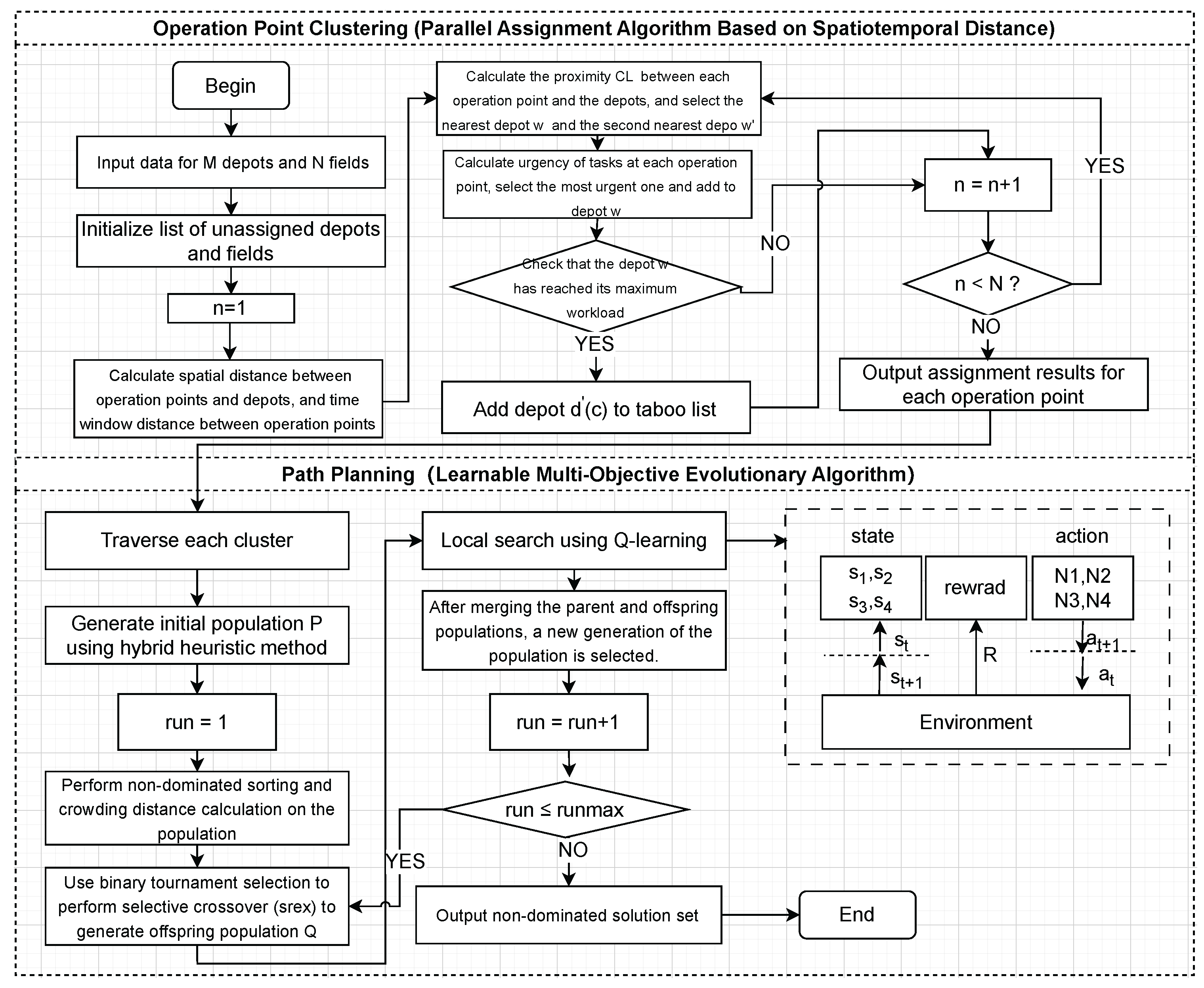
In summary, this paper designs a two-stage scheduling framework starting from order allocation and path planning. To address the limitations of existing order allocation methods that only consider spatial factors, a parallel assignment algorithm based on spatiotemporal characteristics is proposed. This algorithm constructs a temporal distance function to describe the feasibility of continuous operations and evaluates the spatiotemporal proximity of operation points and stations for clustering allocation. Additionally, for the path planning problem, a learnable multi-objective evolutionary algorithm (LMOEA) based on the NSGA-II framework is designed. The algorithm improves the distribution of initial solutions through a hybrid initialization strategy and enhances the diversity of the population with a dynamic crowding distance mechanism. In terms of local search strategy selection, existing methods often use random selection, ignoring the knowledge generated during the evolutionary process. Therefore, we introduce a Q-learning agent to enable the algorithm to learn from the evolutionary process and guide the selection of search strategies, thereby improving the search efficiency of the algorithm.

Our specific work schedule is as follows:

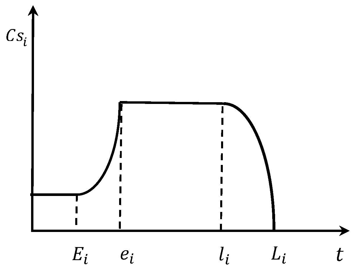
First, we constructed a mathematical model for agricultural machinery operation service scheduling in Section 2.1. In Section 2.1.1, by analyzing the characteristics and influencing factors of the scheduling problem in detail, we clarified the definitions of various parameters and variables in the model and constructed a service satisfaction function based on fuzzy time windows. In Section 2.1.2, we established a multi-objective optimization model aimed at minimizing operational costs and maximizing service satisfaction, and detailed various constraints. Based on this, we introduced a two-stage algorithm framework in Section 2.2 and provided detailed descriptions of each stage in Section 2.3 and Section 2.4. 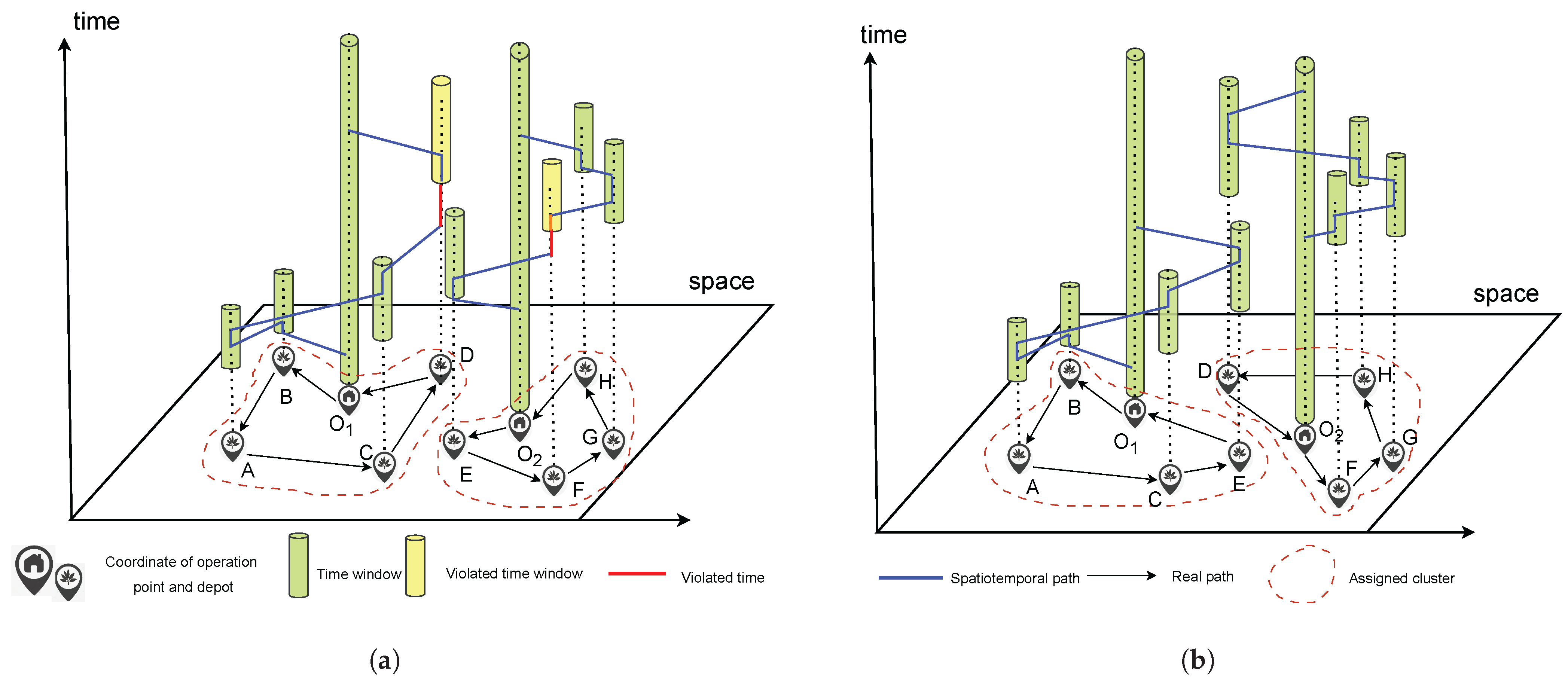Section 2.3 introduced our intelligent allocation of operation demands through an improved parallel assignment algorithm in the first stage, which not only considered traditional spatial distance factors but also introduced a time distance function to evaluate the temporal compatibility between operation points. In Section 2.4, we designed LMOEA in the second stage. LMOEA is based on the NSGA-II algorithm, with improvements in three aspects: initialization (Section 2.4.1), crowding distance calculation (Section 2.4.2), and local search (Section 2.4.3).

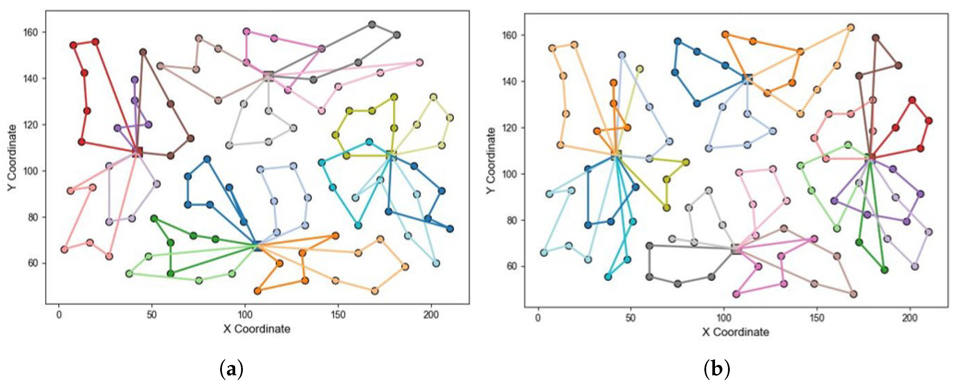
In Section 3.1 and Section 3.2 of the experiments, we defined the instances (datasets) and multi-objective algorithm evaluation criteria, respectively. In Section 3.3, we determined the main hyperparameters of the algorithm through parameter sensitivity experiments of LMOEA. Section 3.4 was designed to verify that the job allocation method based on spatiotemporal clustering in the first stage of Section 2.3 is superior to the job allocation method based on spatial clustering. 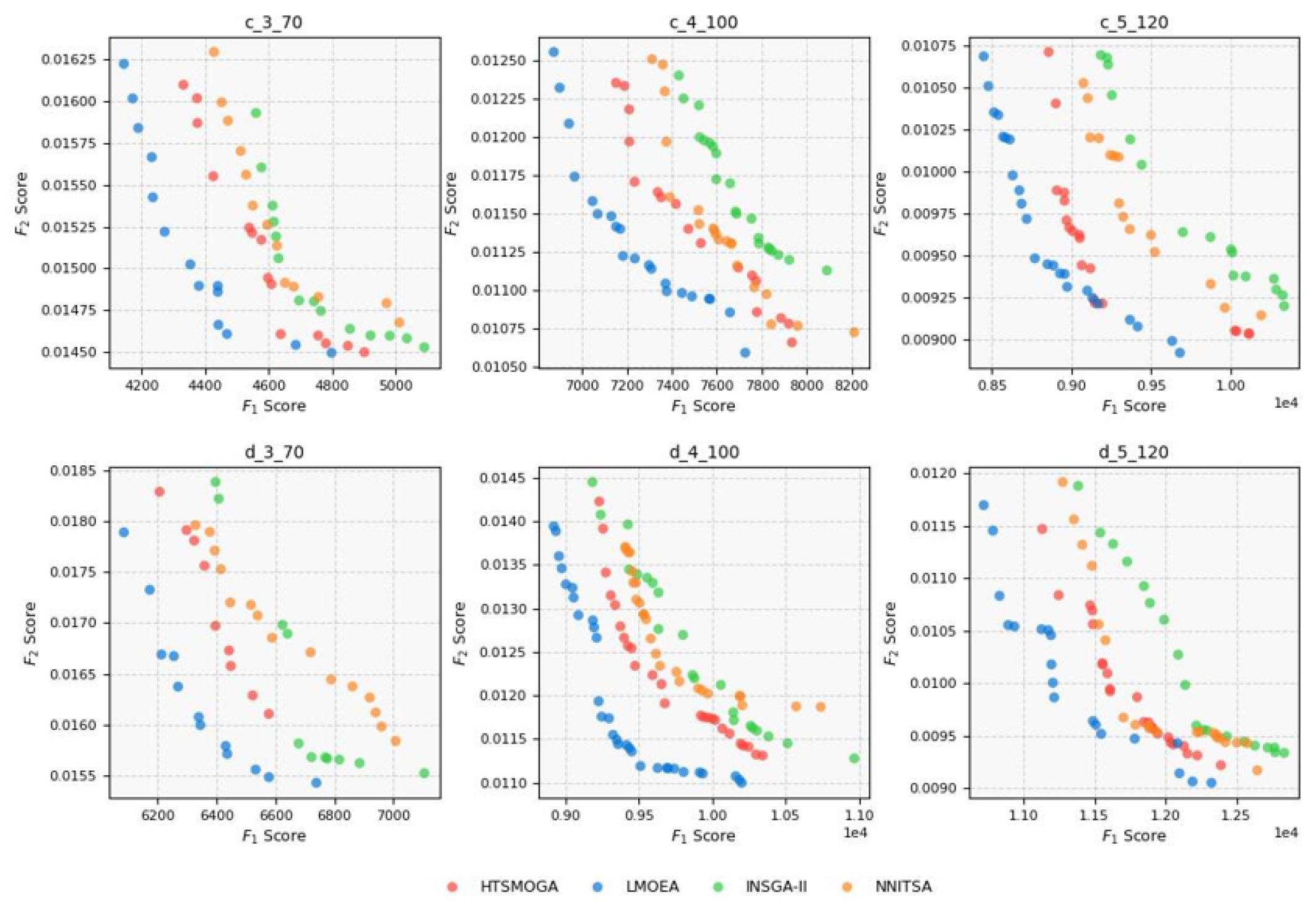Section 3.5 and Section 3.6 were designed to verify that the multi-objective evaluation criteria of LMOEA in the second stage of Section 2.4 are superior to INSGA-II, HTSMOGA, and NNITSA. Section 3.7 is an ablation study corresponding to the improvements of LMOEA in Section 2.4.1, Section 2.4.2, Section 2.4.3.

2. Methods

2.1. Problem Analysis and Objective Functions

2.1.1. Problem Description

The multi-site agricultural machinery operation service scheduling problem involves multiple agricultural machinery service stations and dispersed operation plots. As shown in Figure 1, the scheduling center must consider both the distance between operation plots and service stations, and the availability of agricultural machinery at each station. It must allocate orders to appropriate service stations and develop detailed operation plans to ensure that agricultural machinery completes all tasks along the optimal routes while meeting farmers’ time requirements.

In the actual operation service process, farmers usually have some flexibility regarding operation times and can accept moderate adjustments before or after their desired time windows. Although this temporal flexibility provides more opportunities for optimizing the scheduling scheme, it also increases decision-making complexity.

In response to the aforementioned problem description, this paper makes the following assumptions regarding the model:

1. Special circumstances are not considered: during the scheduling process, we temporarily disregard unpredictable special situations such as extreme weather conditions and field road congestion, which pose additional challenges to the model’s universality and the algorithm’s robustness.

2. Uniform agricultural machinery models and power: it is assumed that all agricultural machinery involved in the scheduling has the same model and known power, meaning that the machinery can maintain a constant speed during transfer and operation, thereby simplifying the calculation of operational efficiency.

3. Ignoring differences in operator experience: we do not consider the potential impact of different operators’ experience on the efficiency of agricultural machinery operations, which helps us focus on the impact of agricultural machinery scheduling itself on operational efficiency.

4. Fixed locations and demands: it is assumed that the locations of all agricultural machinery stations and the demands of the operation points are known and unchanged during the scheduling process, which helps us concentrate on optimizing the scheduling strategy rather than demand forecasting.

5. Single task for agricultural machinery: in one scheduling plan, all agricultural machinery will depart from the station, complete all operational demands, and return to the original warehouse, which helps simplify the path planning problem.

6. Single agricultural machinery operation limit: it is stipulated that a single operation point can only be operated by one piece of agricultural machinery, avoiding the complexity that may arise from multiple machines operating on a single point simultaneously.

7. Uniform dispatching costs: it is assumed that the single dispatching cost of agricultural machinery (including labor costs, startup costs, and maintenance costs) is known, which helps simplify cost calculations and makes the model more manageable.

The efficiency and quality of agricultural machinery operation services are influenced by various factors. Since agricultural machinery scheduling is a variant of the vehicle routing problem (VRP) and falls within the category of NP-hard problems, it is impossible to consider all factors comprehensively and embody them in a mathematical model in the study. Therefore, based on the assumptions made earlier, the key influencing factors analyzed in the model include the following points:

(1) Spatial distribution characteristics. The dispersed distribution of operation plots leads to frequent transfers of agricultural machinery, directly affecting transfer costs and operational efficiency.

(2) Service station resource constraints. The geographical distribution and amount of equipment at agricultural machinery service stations determine the service response capability to surrounding areas.

(3) Time window requirements. The timeliness of crop harvesting requires operations to be completed within specific time windows, which directly affects service quality and farmer satisfaction.

(4) Equipment load limitations. There are upper limits to the continuous operation time and daily operation area of agricultural machinery, which need to be considered in scheduling to avoid excessive loads leading to equipment damage and a decrease in operational quality.

Definitions of relevant parameters based on the problem description are shown in

Table 1. Definition of relevant variables and parameters.

Type	Symbol	Description
Sets	N	Set of all nodes, including depots and operation points, $N=\{1,2,\dots ,n\}$
	$N_D$	Set of agricultural machinery stations, representing the depots where agricultural machinery is stationed, $N_D=\{1,2,\dots ,m\}$
	$N_T$	Set of fields, representing the operation points served, $N_T=\{m+1,\dots ,n\}$
	M	Set of agricultural machinery, representing the available agricultural machinery, $M=\{1,2,\dots ,k\}$
Parameters	$C_1$	Fixed usage cost per piece of agricultural machinery
	$C_2$	Transfer cost per unit distance for each piece of agricultural machinery
	$V_w$	Total amount of agricultural machinery owned by depot w
	$d_{ij}$	Distance from node i to node j
	$v_k$	Transfer speed of agricultural machinery k
	$q_i$	Task demand of operation point i
	$P_k$	Operating power of agricultural machinery k
	$[e_i,l_i]$	Expected completion time window for operation point i
	$[E_i,L_i]$	Acceptable time window for operation point i
	$T_{max}$	Maximum working time of agricultural machinery within a scheduling period
	$Q_k$	Maximum workload of agricultural machinery k within a scheduling period
Variables	$X_{ijk}$	Binary variable, indicating whether agricultural machinery k transfers from node i to node j
	$Z_{wk}$	Binary variable, indicating whether agricultural machinery k departs from depot w
	$Y_{ik}$	Binary variable, indicating whether operation point i is assigned to agricultural machinery k
	$A{T}_{ik}$	Time at which agricultural machinery k arrives at operation point i
	$L{T}_{ik}$	Time at which agricultural machinery k leaves operation point i
	$S{T}_{ik}$	Waiting time of agricultural machinery k at operation point i
	$S_{ik}$	Operating time of agricultural machinery k at operation point i
	$t_{ijk}$	Transfer time of agricultural machinery k from operation point i to operation point j

.

Agricultural machinery operation services are typical examples of agricultural socialized services. One of the core indicators for evaluating their quality is farmer satisfaction. Since agricultural production has strict requirements for timing, missing the optimal farming time can directly affect crop yield and quality. Therefore, the timeliness of operations becomes a decisive factor affecting farmer satisfaction. To effectively utilize this relationship in the optimization model, it is necessary to transform the subjective evaluation of timeliness by farmers into a quantifiable mathematical expression. In the actual operation service process, although farmers have a preferred operation time window, they also have a certain tolerance for the early or delayed arrival of agricultural machinery. This temporal flexibility depends on the growth characteristics of the crops, weather conditions, and the farmers’ own production arrangements. Therefore, this paper designs a satisfaction function based on fuzzy time windows [27].

As depicted in Figure 2, the acceptable service time frame $[E_i,L_i]$ for farmers is segmented into several intervals. The interval $[e_i,l_i]$ represents the optimal operating window preferred by farmers, during which agricultural machinery arriving at the operation site achieves the highest satisfaction level of 1. The interval $[E_i,e_i]$ indicates the time range within which operations can be advanced, with satisfaction changes described by an exponential function that reflects the accelerated deterioration of impacts due to early operations (such as crops not being in the optimal state or inadequate farmer preparation) as time increases. The interval $[l_i,L_i]$ is the time range within which operations can be delayed, and considering the characteristics of crop quality decline and increased losses after the optimal harvest period, the satisfaction function decreases using a power function. Parameters k and $K_i$ can adjust the sensitivity of the function to accommodate the time-sensitive characteristics of different scheduling plans. This nonlinear change in satisfaction more closely aligns with real-world scenarios, as shown in Equation (1).

$$c{s}_i\left(A{T}_{ik}\right)=\left\{\begin{array}{cc}expK\left(E_i-e_i\right),\hfill & A{T}_{ik}<E_i\hfill \\ expK\left(A{T}_{ik}-e_i\right),\hfill & E_i<A{T}_{ik}<e_i\hfill \\ 1,\hfill & e_i<A{T}_{ik}<l_i\hfill \\ 1-{\left({\displaystyle \frac{A{T}_{ik}-l_i}{L_i-l_i}}\right)}^{K_i},\hfill & l_i<A{T}_{ik}<L_i\hfill \\ 0,\hfill & A{T}_{ik}>L_i\hfill \end{array}\right.$$

(1)

2.1.2. Objective Functions and Constraints

(1) Objective Function

In agricultural machinery operation services, since the area of the fields and the operating power of the agricultural machinery remain constant during the scheduling process, and the unit operating efficiency of the same type of machinery is essentially the same, the operating cost and time for each field can be considered fixed values without accounting for losses. The core of scheduling optimization lies in solving the transfer planning problem of agricultural machinery between different fields, which involves two key cost factors: first, the transfer cost from one field to another, and second, the usage cost directly related to the number of agricultural machines scheduled. Each piece of machinery requires a dedicated operator. This labor cost is relatively fixed. Additionally, relevant studies have shown that the maintenance cost of a single piece of agricultural machinery during the scheduling process accounts for about 20% to 30% of the operating cost [28]. Therefore, reducing the number of agricultural machines used can not only lower equipment maintenance costs but also significantly save on fixed labor expenses. Based on this, this study aims to optimize the scheduling plan to achieve the goals of minimizing transfer distance and the number of agricultural machines used. The cost optimization objective is shown in Equation (2).

$$F_1=C_1\sum _{k\in M}{Z}_{wk}+C_2\sum _{i\in N_T}\sum _{j\in N_T}{x}_{ijk}·d_{ij}$$

(2)

This study utilizes the reciprocal of the sum of all farmers’ satisfaction levels as an additional optimization objective. By minimizing this value, the overall service satisfaction is maximized, as shown in Equation (3).

$$F_2={\displaystyle \frac{1}{{\sum }_{i\in N_T}{\sum }_{k\in M}c{s}_i\left(A{T}_{ik}\right)}}$$

(3)

(2) Constraints

Equations (4) and (5) represent the visitation constraints for the operation points, ensuring that each field can be serviced by only one piece of agricultural machinery and that it is visited exactly once.

$$\sum _{k\in M}{Y}_{ik}=1,\forall i\in N_T$$

(4)

$$\sum _{j\in N}{X}_{ijk}\le 1,\forall i\in N_T,k\in M$$

(5)

Equation (6) represents the flow conservation constraint, which ensures that the number of agricultural machines entering and leaving each field is consistent.

$$\sum _{j\in N}{X}_{ijk}=\sum _{j\in N}{X}_{jik},\forall i\in N_T,k\in M$$

(6)

Equations (7) and (8) are designed to ensure that all agricultural machinery departs from the depot at the start of the tasks and returns to the original depot after all tasks are completed.

$$\sum _{j\in N}{X}_{ijk}=\sum _{w\in N_D}{Z}_{wk},\forall i\in N_T,k\in M$$

(7)

$$\sum _{w\in N_D}{Z}_{wk}=1,k\in M$$

(8)

Equation (9) imposes a constraint that the number of agricultural machines used from each depot must not exceed the number of machines available at that depot.   

$$\sum _{k\in M}{Z}_{wk}\le V_w,\forall w\in N_D$$

(9)

Equations (10) and (11) impose constraints on the working hours and the amount of work each piece of agricultural machinery can handle within a single scheduling period.

$$\sum _{i\in N}\left(S_{ik}·X_{ijk}\right)+t_{ijk}·X_{ijk}\le T_{max},k\in M$$

(10)

$$\sum _{i\in N_T}{q}_i{Y}_{ik}\le Q_k$$

(11)

Equations (12) and (13) are constraints on the service start time of agricultural machinery. If the service starts earlier than the acceptable earliest service time, the machinery must wait and cannot exceed the latest acceptable service time set by the farmers.

$$E_i\le S{T}_{ik}<L_i,\forall i\in N_T,k\in M$$

(12)

$$S{T}_{ik}=max\left(E_i,A{T}_{ik}\right),\forall i\in N_T,k\in M$$

(13)

Equations (14) and (15) are constraints related to the transfer time and service time of agricultural machinery.

$$S_{ik}={\displaystyle \frac{q_i}{p_k}},\forall i\in N_T,k\in M$$

(14)

$$t_{ijk}={\displaystyle \frac{d_{ij}}{v_k}},\forall i,j\in N,k\in M$$

(15)

Equations (16)–(18) are constraints on the decision variables.

$$X_{ijk}\in \{0,1\},\forall i,j\in N,k\in M$$

(16)

$$Y_{ik}\in \{0,1\},i\in N_T,k\in M$$

(17)

$$Z_{wk}\in \{0,1\},w\in N_D,k\in M$$

(18)

2.2. Design of a Two-Stage Solution Algorithm Framework

Agricultural machinery operation services are essentially a type of multi-depot agricultural machinery scheduling problem with fuzzy time windows. Compared to single-depot scheduling, this problem presents higher complexity and challenges. For such multi-depot scheduling problems, customer clustering methods have been proven to be significantly effective [29,30,31]. By clustering customer demands, the search space in the path planning phase can be effectively reduced, significantly lowering computational complexity and aiding in the regionalized scheduling and allocation of agricultural machinery resources.

Agricultural machinery operation service scheduling can be considered an extension of the VRP and is classified as an NP-hard problem. Due to the complexity of the problem, solving it with exact algorithms poses significant challenges. NSGA-II [32], as a multi-objective evolutionary algorithm, has demonstrated excellent performance in solving multi-objective vehicle path optimization problems. This algorithm ensures robust global search capabilities through a fast non-dominated sorting mechanism and effectively maintains diversity in the solution space using a crowding distance calculation method.

Based on the above analysis, this paper proposes a two-stage algorithm framework, as shown in Figure 3, combining customer clustering with a LMOEA. The first stage designs a parallel assignment algorithm based on spatiotemporal distance, intelligently assigning operation demands to various depots based on temporal and spatial characteristics. The second stage, building on the NSGA-II algorithm framework, integrates hybrid initialization methods and learnable local search strategies, proposing a LMOEA for optimizing the path planning after assignment.

2.3. Parallel Assignment Algorithm Based on Spatiotemporal Distance

In multi-depot agricultural machinery scheduling, each station often has a limited number of machines and varying service capabilities. Therefore, clustering and assigning tasks according to order requirements are essential to improve overall resource utilization efficiency. The order assignment strategy directly affects the optimization of subsequent path planning; a reasonable allocation plan can provide more feasible solutions for path planning, enhancing the overall service quality of the scheduling scheme.

Existing research primarily considers order assignment from a spatial distance perspective, often using distance-based clustering methods or nearest-depot assignment strategies. While these methods can assign operation points that are geographically close to the same service station, they often overlook the constraints of the operation time windows. As shown in Figure 4a, although operation points are assigned to the nearest agricultural machinery station during the assignment process, the service times of points D and F are highly mismatched with those of other operation points at depots $O_1$ and $O_2$. This leads to prolonged idling of agricultural machinery, resulting in resource wastage. In contrast, Figure 4b shows a more rational work group formed after considering temporal factors, shortening the cycle time to complete all tasks in the route, which is particularly important during resource-scarce peak farming periods.

Giosa proposed a parallel assignment algorithm for the multi-depot vehicle scheduling problem [33]. The algorithm determines the assignment order by evaluating the urgency (priority) of each task point, prioritizing the allocation of high-urgency task points to depots with sufficient service capacity. The calculation of urgency is primarily based on the spatial distance from the task point to the depot.

The specific calculation of urgency is shown in Equation (19), where $d(c,dep)$ represents the distance between the depot and task point c, and $d(c,de{p}^{\prime })$ represents the distance between task point c and the nearest depot.

$$U\left(c\right)=\sum _{dep\in N_D}\left[d(c,dep)-d(c,de{p}^{\prime })\right]$$

(19)

Additionally, to reduce computational complexity, the parallel assignment algorithm employs a simplified calculation method, which only considers the nearest and second-nearest depots during the urgency calculation, as shown in Equation (20).

$$U\left(c\right)=d(c,de{p}^{″})-d(c,de{p}^{\prime })$$

(20)

The parallel assignment algorithm, in evaluating the urgency of completing task points, still considers only spatial distance factors in the allocation process. To address the shortcomings of previous methods, we improve the calculation of algorithm urgency $U\left(c\right)$ by designing a spatiotemporal distance function. This function differs from traditional spatial distance metrics as it comprehensively considers driving time, waiting time, and delay time across multiple temporal dimensions, to assess the temporal feasibility of performing consecutive operations between two task points. This improvement allows the scheduling system to balance spatial and temporal constraints simultaneously during task allocation, thereby reducing the occurrence of agricultural machinery idling or order delays. Suppose the operation points i and j have time windows $[E_i,L_i]$ and $[E_j,L_j]$, respectively. Then, the arrival time of agricultural machinery k from i to j is $A{T}_{kj}\in [E_i+S_{ik}+t_{ijk},L_i+S_{ik}+t_{ijk}]$, and is set as $[ET,LT]$. The $[ET,LT]$ has several relationships with the time window of operation point j, as shown in Figure 5.

If $LT<E_j$, it indicates that agricultural machinery k completes its operation at point i and arrives at operation point j after the earliest acceptable operation time for the farmer, requiring waiting before starting the operation. At this time, the temporal distance is represented as the sum of transfer time and waiting time, which can be expressed as $E_j-LT+t_{ijk}$.

If $ET<e_j\le LT$, it indicates that agricultural machinery k may arrive at operation point j earlier than the earliest acceptable operation time for the farmer. At this time, the calculation is made as ${\omega }_1(E_j-LT)+t_{ijk}$, where ${\omega }_1$ is a waiting time bias coefficient, represented as ${\displaystyle \frac{E_j-ET}{LT-ET}}$. The larger ${\omega }_1$ is, the higher the likelihood of agricultural machinery k waiting at point j, and the higher the penalty.

If $ET\le e_j<l_j\le LT$, it indicates that the possible arrival time range of agricultural machinery k at point j is completely within the time window of operation point j, and agricultural machinery can start the operation on time. At this time, the temporal distance is directly represented as the transfer time ($t_{ijk}$) between i and j.

If $ET\le l_j<LT$, it indicates that there is a possibility of delay for agricultural machinery k arriving at operation point j. The handling method is similar to the second situation, introducing a delay penalty coefficient ${\omega }_2$, and at this time the temporal distance is represented as ${\omega }_2(LT-L_j)+t_{ijk}$, and ${\omega }_2$ can be expressed as ${\displaystyle \frac{LT-L_j}{LT-ET}}$.

If $ET>L_j$, then agricultural machinery k will definitely be delayed when arriving at point j, at which time the temporal distance is represented as the sum of delay time and transfer time, which can be expressed as $LT-L_i+t_{ijk}$, the sum of delay time and transfer time.

Summing up the above, by considering the five scenarios, the temporal distance can be summarized as Equation (21).

$$D_{ij}^T=\left\{\begin{array}{cc}{E}_j-LT+t_{ijk},\hfill & LT<E_j\hfill \\ {\displaystyle \frac{{(E_j-ET)}^2}{(LT-ET)}}+t_{ijk},\hfill & ET<E_j\le LT\hfill \\ t_{ijk},\hfill & ET\le E_j<L_i\le LT\hfill \\ {\displaystyle \frac{{(LT-L_j)}^2}{LT-ET}}+t_{ijk},\hfill & ET<L_i<LT\hfill \\ LT-L_i+t_{ijk},\hfill & ET<L_j\hfill \end{array}\right.$$

(21)

Based on the above temporal distance function, the closeness between operation points and various stations in terms of time can be calculated by Equation (22), which evaluates the time feasibility of operation points i and those already assigned to station w in the continuous operation process.

$$AF(i,w)=\left\{{\displaystyle \frac{{\sum }_{j\in N_T\left(w\right)\cup \left\{w\right\}}{e}^{-D_{ij}^T}}{|N_T|}}\right\},i,j\in N_T,w\in N_D$$

(22)

The proximity of operation point i to depot w can be calculated by Equation (23), which comprehensively considers both temporal and spatial factors.

$$CL(i,w)={\displaystyle \frac{d(i,w)}{AF(i,w)}},i\in N_T,w\in N_D$$

(23)

The urgency of operation point i after improvement can be represented by Equation (24), where w and $w^{\prime }$ are the two depots with the smallest and second smallest proximity, respectively.

$$U\left(i\right)=CL(i,w^{\prime })-CL(i,w),w,w^{\prime }\in N_D$$

(24)

Based on the above improvements, this chapter quantifies the time compatibility of operation points and stations through index transformation and value normalization, achieving self-adaptation of temporal and spatial constraints, increasing the likelihood that operation points with higher temporal compatibility are assigned to their corresponding stations.

2.4. Learnable Multi-Objective Evolutionary Algorithm

To address the agricultural machinery path optimization problem under time window constraints, we propose a Learnable Multi-Objective Evolutionary Algorithm (LMOEA) built upon the NSGA-II framework. While preserving its core components—including fast non-dominated sorting, crowding distance calculation, and elite preservation—LMOEA introduces three key improvements. First, a hybrid initialization strategy is employed to enhance population quality. Second, a reinforcement learning-based local search module is integrated to adaptively guide search behavior and reduce ineffective iterations. Third, a dynamically adjusted crowding distance mechanism is designed to promote better distribution across the Pareto front. The overall procedure is illustrated in Algorithm 1.

Algorithm 1 Learnable Multi-objective Evolutionary Algorithm (LMOEA)

Input:  Population size N, crossover rate $P_c$, local search rate $P_l$, maximum generation $G_{max}$, discount factor $\gamma$, learning rate $\alpha$ Output:  Non-dominated solution set $PS$   1: Generate initial population P using a hybrid initialization strategy   2: Initialize Q-table, set exploration rate $\epsilon$   3: Evaluate population: perform non-dominated sorting and crowding distance calculation on P   4: for $g=1$ to $G_{max}$ do   5:     for $i=1$ to $N/2$ do   6:         Select parents $\{p_1,p_2\}$ via binary tournament selection on P   7:         Generate offspring: $O\leftarrow O\cup \mathrm{SREX}(\{p_1,p_2\},P_c)$   8:     end for   9:     Combine population: $R\leftarrow P\cup O$ 10:     for each individual $x\in R$ do 11:       if $\mathrm{rand}\left(\right)<P_l$ then 12:            Use $\epsilon$-greedy strategy to select and perform a neighborhood operator 13:            Update Q-table 14:       end if 15:    end for 16:    $P\leftarrow \mathrm{popUpdate}(R,N)$ Select next generation based on non-dominated sorting and dynamic crowding distance 17:    Update $\epsilon$: $\epsilon \leftarrow f(\epsilon ,g)$ 18: end for 19: return $PS$

2.4.1. Hybrid Initialization Method

This study employs a hybrid initialization method aimed at overcoming the limitations of a single initialization strategy by generating a diversified and high-quality initial solution to enhance the overall performance and stability of the algorithm. This method divides the initial population according to the ratio of 4:3:3, using random initialization, the plane-sweeping algorithm [34], and an improved k-nearest-neighbors algorithm (KNN) [35]. This proportional allocation ensures both diversity and quality of the initial solution.

The plane-sweeping algorithm originates from the line segment intersection problem in computational geometry, with the core idea of transforming a two-dimensional plane problem into a one-dimensional sweep problem. In the operation area division, this algorithm uses agricultural stations as vertices, dividing adjacent customer points into the same area through a clockwise rotation sweep, as shown in Figure 6. To obtain a high-quality delivery route initial solution, this paper modifies the traditional plane-sweeping algorithm, completing area division while using insertion heuristics to construct the delivery route. This simultaneous optimization strategy ensures both geographical continuity and solution feasibility. The specific process is as follows:

• Step 1: Draw a circle centered at the agricultural station O to cover all operation points, convert each operation point to polar coordinates $(r,\theta )$, and randomly select an operation point as the starting point.
• Step 2: Sweep the area in polar order and add operation points to the region, calculate the optimal insertion position for each new point, and update the delivery route to ensure it meets the operation limit and time window constraints.
• Step 3: When no new operation points can be inserted, complete the current area division and route construction, and start the construction process for the next area.
• Step 4: Repeat steps 2–3 until all operation points are assigned and the route construction is complete.

To consider the operation time window factor in the initialization process, this paper combines the KNN algorithm to design an initialization algorithm. In the VRP, the basic principle of the KNN algorithm is to select the nearest k operation points based on distance and randomly choose one to add to the route. In this paper, k neighboring operation points are calculated based on Equation (25) for selection, where the spatial distance and temporal distance are normalized and weighted to ensure that the selection of operation points considers both spatial and temporal characteristics. In this paper, $\alpha$ is taken as 0.5.

$$D_{ij}^{ST}=\alpha {\displaystyle \frac{D_{ij}^S-min{D}^S}{max{D}^S-min{D}^S}}+(1-\alpha ){\displaystyle \frac{D_{ij}^T-min{D}^T}{max{D}^T-min{D}^T}}$$

(25)

2.4.2. Non-Dominated Sorting and Dynamic Crowding Distance Calculation

The algorithm achieves the selection of elite individuals in each round through non-dominated sorting and crowding distance, where non-dominated sorting is used to evaluate the quality of individuals, and crowding distance is used to maintain population diversity. The specific implementation process is as follows:

• Step 1: Merge the parent population $P\left(t\right)$ and the offspring population $Q\left(t\right)$ to form a population $R\left(t\right)$ with a size of $2N$.
• Step 2: Perform fast non-dominated sorting on population $R\left(t\right)$ to obtain non-dominated layers $L=\{L_1,L_2,\dots ,L_n\}$.
• Step 3: In the order of non-dominated levels, start from $L_1$ and select individuals to construct a new population until the population size reaches N.
• Step 4: For the non-dominated layers $L_i$ that cannot be fully added, select individuals based on crowding distance $d_j$ in descending order.

In the above algorithm, when a non-dominated layer cannot be completely added to the new population, it is necessary to select individuals from this layer based on crowding distance. However, traditional methods only complete the removal of multiple individuals through a single crowding distance sorting, and then remove the solution with the smallest crowding distance.

To overcome the shortcomings in the above individual removal process, this paper designs a simple but effective dynamic crowding distance sorting method: whenever the smallest individual $x_i$ in the current non-dominated layer is removed, before selecting the next individual to remove, update the crowding distance of its neighboring solutions $x_{i-1}$ and $x_{i+1}$ as the new sorting results to ensure that the crowding distance ranking always reflects the current distribution of the solution. As shown in Figure 7a, before $x_i$ is removed, the crowding distance (Dist) between neighboring individuals $x_{i-1}$ and $x_{i+1}$ is calculated as follows:

$$\left\{\begin{array}{c}{d}_k\left(x_{i-1}\right)={\displaystyle \frac{|f_k\left(x_i\right)-f_k\left(x_{i-2}\right)|}{max\left(f_k\right)-min\left(f_k\right)}}\hfill \\ Dist\left(x_{i-1}\right)=\sum _{k=1}^m{d}_k\left(x_{i-1}\right)\hfill \end{array}\right.$$

(26)

$$\left\{\begin{array}{c}{d}_k\left(x_{i+1}\right)={\displaystyle \frac{|f_k\left(x_i\right)-f_k\left(x_{i+2}\right)|}{max\left(f_k\right)-min\left(f_k\right)}}\hfill \\ Dist\left(x_{i+1}\right)=\sum _{k=1}^m{d}_k\left(x_{i+1}\right)\hfill \end{array}\right.$$

(27)

After removing individual $x_i$, as shown in Figure 7b, the crowding distances of neighboring solutions $x_{i-1}$ and $x_{i+1}$ change, and their crowding distances $Dist$ are calculated by Equations (28) and (29).

$$\left\{\begin{array}{c}{d}_k\left(x_{i-1}\right)={\displaystyle \frac{|f_k\left(x_{i+1}\right)-f_k\left(x_{i-2}\right)|}{max\left(f_k\right)-min\left(f_k\right)}}\hfill \\ Dist\left(x_{i+1}\right)=\sum _{k=1}^m{d}_k\left(x_{i-1}\right)\hfill \end{array}\right.$$

(28)

$$\left\{\begin{array}{c}{d}_k\left(x_{i+1}\right)={\displaystyle \frac{|f_k\left(x_{i-1}\right)-f_k\left(x_{i+2}\right)|}{max\left(f_k\right)-min\left(f_k\right)}}\hfill \\ Dist\left(x_{i+1}\right)=\sum _{k=1}^m{d}_k\left(x_{i+1}\right)\hfill \end{array}\right.$$

(29)

By using this method, after removing each solution, only the crowding distance of its neighboring solutions needs to be updated, without the need to recalculate the crowding distance of all solutions, thus reducing computational complexity. At the same time, it improves the problem of uneven distribution of solutions caused by inaccurate crowding distance sorting.

2.4.3. Local Search Strategy Based on Q-Learning

This paper uses the Selective Route Exchange Crossover (SREX) operator for the crossover operation of the algorithm. The selection of individuals is based on the binary tournament method. Local search is a key technology to improve the efficiency of algorithm exploration and promote population diversity, effectively preventing the algorithm from falling into local optima [36]. However, in traditional methods, executing multiple neighborhood operators one by one takes too long, and random selection of operators leads to low success rates. To address these issues, this paper designs an adaptive local search method based on Q-learning, as illustrated in Figure 8. By considering the current state and historical performance of individuals, appropriate neighborhood operators are dynamically selected at each search step.

Q-learning, as a classic reinforcement learning algorithm, has been widely applied in the field of scheduling. This algorithm typically consists of five elements: Agent, Environment, Action, State, and Reward. Its core mechanism is to maintain a Q-table to record the long-term cumulative reward for each state-action pair. In this paper, each individual in the population $X=\{x_1,x_2,\dots ,x_n\}$ of size N is considered an intelligence entity. The state reflects the current adaptability of the individual, and the action corresponds to the available neighborhood operators. At each search step, the intelligence entity senses the current state, selects the optimal neighborhood operator based on the Q-table, executes it, then obtains the corresponding reward, and transitions to a new state. By continuously updating the values in the Q-table, it can continuously optimize the selection of neighborhood operators for individuals under different environments. The update formula for the Q-table is:

$$Q(s_t,a_t)=(1-\alpha )·Q(s_t,a_t)+\alpha ·(r_t+\gamma ·maxQ(s_{t+1},a))$$

(30)

State Design: Considering the complexity of solving the combined optimization problem, directly using the structure characteristics of the solution space as the state representation may lead to a dimensionality disaster. Therefore, this paper proposes a state representation method based on the target space, dividing the solution space into four quadrants to simplify the state representation. The specific division process is as follows:

• Step 1: Sort all individuals in the population by $f_1$ value in ascending order and calculate the median $f_1^{Med}=f_1\left(x_{N/2}\right)$.
• Step 2: Use the same method to sort by $f_2$ value and calculate the median $f_2^{Med}$.
• Step 3: Use $f_1^{Med}$ and $f_2^{Med}$ as boundaries to divide the target space into four quadrants, each quadrant representing a state.

This method of dividing the solution space based on medians has the following advantages: First, it disperses the continuous target space into four states, significantly reducing the complexity of the state space; second, it divides the target space by the median of the population’s objective values, ensuring that each quadrant contains approximately equal numbers of individuals, maintaining the balance of the state division; finally, this dynamic partitioning method can adapt to the evolution process, better reflecting the distribution characteristics of the current population.

Table 2. State judgment condition.

State	Description	State	Description
1	$f_1\left(x_i\right)\le f_1^{Med}\wedge f_2\left(x_i\right)\le f_2^{Med}$	3	$f_1\left(x_i\right)\le f_1^{Med}\wedge f_2\left(x_i\right)\le f_2^{Med}$
2	$f_1\left(x_i\right)\le f_1^{Med}\wedge f_2\left(x_i\right)>f_2^{Med}$	4	$f_1\left(x_i\right)\le f_1^{Med}\wedge f_2\left(x_i\right)>f_2^{Med}$

provides the specific conditions for the four states.

Reward Function: After each training session, each neighborhood selection action is rewarded based on the improvement effect of the individual. In this paper, the reward function is calculated based on the comprehensive improvement effect on multiple optimization objectives, and can be defined as:

$$r_t=max\left(\sum _{k=1}^K{\displaystyle \frac{f_k^{min}}{f_k\left(x_t\right)}}\left({\displaystyle \frac{f_k\left(x_{t-1}\right)-f_k\left(x_t\right)}{f_k^{max}-f_k^{min}}}\right),0\right)$$

(31)

where $f_k^{max}$ and $f_k^{min}$ represent the maximum and minimum values found for the k-th optimization objective, respectively. $x_{t-1}$ denotes the initial solution, and $x_t$ is the new solution obtained by the neighborhood search. According to Equation (31), the larger the target function improvement, the the closer to the current optimal solution, the greater the reward. Additionally, negative feedback will reduce the impact of successful rewards, making the positive reward more prominent. When the comprehensive improvement of the new solution is negative, the reward is set to 0 without punishment.

Strategy: To balance exploration of new actions and exploitation of known optimal actions, this algorithm adopts the $\epsilon$-greedy strategy [37]. Specifically, at each decision step, an action is selected at random with probability $\epsilon$ (exploration), and with probability $1-\epsilon$, the action with the highest Q-value under the current state is selected (exploitation). The value of $\epsilon$ gradually decreases with the generation index g, enabling the algorithm to smoothly transition from exploration to exploitation as learning progresses.

Actions: As shown in Figure 9, this paper uses six neighborhood search operators as the action set in Q-learning, and adopts the acceptance rule based on the Pareto optimality principle: when a new solution $x^{\prime }$ dominates the current solution x, it is directly accepted; when $x^{\prime }$ is non-dominated by x, it is accepted with a probability of 0.5. This strategy ensures that the quality of the solution will not decrease while providing sufficient exploration capability to escape from local optima. The neighborhood operators are designed as follows:

• Swap: Exchange the positions of two nodes in the same or different paths.
• 2-opt: Select two non-adjacent edges in the path, break them, and reconnect them in reverse order.
• Relocate: Move a node from its initial position to a new position in the same or different path.
• 2-Relocate: Move two consecutive nodes from their original positions to new positions in the same or different paths.
• Arc-Swap: Exchange two consecutive node sequences in the same or different paths.
• Path-Remove: Randomly remove a node sequence from a path and insert it into another path.

3. Experimental Verification and Analysis

3.1. Instance Description

Based on the characteristics of the two types of operation requirements, this study designs two categories of a total of 12 test instances to verify the effectiveness of the proposed algorithm. These instances are constructed based on representative real-world patterns, partially illustrated in

Table 3. Operation point information.

Operation Point	Coordinates	Operation Area (ha)
1	(89.62337080817368,43.83519517958557)	0.79
2	(89.60990291336401,43.83225298520169)	0.71
3	(89.62373851155712,43.83415198062051)	2.13
4	(89.6042680311066,43.82290470780433)	2.38
5	(89.60491842829208,43.82276405036669)	2.25
6	(89.60771369608014,43.82180446148496)	1.87
7	(89.61970346331935,43.82041586887333)	1.62
8	(89.61400475918953,43.81625195121295)	1.57
9	(89.61947175127257,43.81600461431319)	1.68
10	(89.61992756569268,43.81601290031301)	1.21
...

, which displays information for the first ten operation points. Each instance is labeled using the format “feature type—number of operation points—number of service stations” and includes both C-type and D-type cases, where the number of operation points $N\in \{45,70,80,100,120,160\}$ and the corresponding number of service stations $M\in \{2,3,4,4,5,5\}$. Among them, C-type instances correspond to large-scale farms, where farmland is spatially clustered and fields within the same cluster typically belong to the same farmer or cooperative. These instances feature relatively relaxed time windows (1–3 days) and similar operation time requirements within clusters. In contrast, D-type instances represent smallholder farms, which are uniformly scattered and subject to more varied and tighter time constraints. Their operation windows are limited to specific periods within a day (e.g., [480, 720] denotes 8:00–12:00).

The farmland areas of the two types of test instances are all between 0.5 and 2.5 hectares. Each service station is randomly assigned 5 to 10 seeding machines, which are uniformly configured with the same operational parameters. Additionally, the parameters of the agricultural machines during the experiment are set as shown in

Table 4. Agricultural machinery parameter settings.

Parameter	Description	Default Value
$P_k$	Agricultural machinery operation efficiency (ha/h)	0.45
$V_k$	Agricultural machinery transfer speed (km/h)	40
$T_{max}$	Maximum working time of agricultural machinery (h/d)	12
$C_1$	Single dispatch cost of agricultural machinery (Yuan)	300
$C_2$	Unit distance transfer cost (Yuan/km)	2

.

3.2. Evaluation Metrics

The hypervolume (HV) calculates the multidimensional space volume formed by the non-dominated solution set and reference points [38]. For the minimization problem, given a non-dominated solution set P and a reference point r, HV can be represented as:

$$HV(P,r)=\Lambda \left(\bigcup _{x\in P}\left[f_1\left(x\right),r_1\right]\times \dots \times \left[f_m\left(x\right),r_m\right]\right)$$

(32)

where $\Lambda$ represents the Lebesgue measure (in two dimensions it is the area), $f\left(x\right)$ represents the function value of solution x on the i-th objective, $r_i$ represents the coordinate of the reference point on the i-th dimension, and m is the number of objectives. The larger the HV value, the better the algorithm’s performance, as it reflects both the convergence and diversity of the solution set. To eliminate the impact of different objective scales, the reference point is chosen as $[1,1]$ after normalization before calculating HV.

The inverted generational distance (IGD) measures the proximity of the non-dominated solution set obtained by the algorithm to the true Pareto front [39]. Given a set $P*$ uniformly distributed along the true Pareto front and the non-dominated solution set P obtained by the algorithm, IGD is defined as:

$$IGD(P,P*)={\displaystyle \frac{{\sum }_{v\in P*}d(v,p)}{|P*|}}$$

(33)

where $d(v,P)$ represents the Euclidean distance from v to the nearest point in set P. The smaller the IGD value, the closer the solution set obtained by the algorithm is to the true Pareto front, indicating better performance.

3.3. Algorithm Parameter Settings

To determine the optimal parameter configuration for the LMOEA algorithm, this section uses the Taguchi method [40] on the four key parameters of the algorithm: crossover probability $P_c$, local search probability $P_l$, learning rate $\alpha$, and discount factor $\gamma$. Each parameter is set at three levels: crossover probability $P_c$ is set to 0.3, 0.5, and 0.7; local search probability $P_l$ is set to 0.2, 0.3, and 0.4; learning rate $\alpha$ is set to 0.1, 0.2, and 0.3; discount factor $\gamma$ is set to 0.7, 0.8, and 0.9. The experiment uses an L9 ($3^4$) orthogonal array (as shown in

Table 5. Parameter settings and HV values.

No.	${\mathit{P}}_{\mathit{c}}$	${\mathit{P}}_{\mathit{l}}$	$\mathit{\alpha }$	$\mathit{\gamma }$	HV
1	0.3	0.2	0.1	0.7	0.5371
2	0.3	0.3	0.2	0.8	0.4793
3	0.3	0.4	0.3	0.9	0.4996
4	0.5	0.2	0.2	0.9	0.5878
5	0.5	0.3	0.3	0.7	0.6193
6	0.5	0.4	0.1	0.8	0.6501
7	0.7	0.2	0.3	0.8	0.4015
8	0.7	0.3	0.1	0.9	0.6892
9	0.7	0.4	0.2	0.7	0.5292

), and each parameter combination is run independently 20 times to ensure the statistical reliability of the experiment.

Figure 10 shows the main effects of each parameter on the average HV value. By calculating the average HV values of each parameter at different levels, it can be observed that the crossover probability $P_c$ and the local search probability $P_l$ have a greater impact on the algorithm’s performance, with the optimal values being 0.5 and 0.3, respectively. The learning rate $\alpha$ achieves the best results at 0.1, indicating that a smaller learning rate is beneficial for the stability of the algorithm; the discount factor $\gamma$ achieves the best results at 0.9, indicating that the algorithm is more inclined to consider long-term benefits. Based on the main effect analysis, the parameter configuration of the algorithm is determined as: $P_c=0.5$, $P_l=0.3$, $\alpha =0.1$, and $\gamma =0.9$. This parameter combination will be used for subsequent experiments.

3.4. Validation of Allocation Strategy Effectiveness

To verify the advantages of the improved parallel assignment algorithm proposed in this paper for the multi-depot scheduling process in the order aggregation process, two allocation strategies based on spatial distance and spatiotemporal distance are applied in each test case, respectively. The same LMOEA algorithm is used for subsequent path planning. To ensure the statistical reliability of the results, each test case is run independently 20 times, and the best solution is selected for comparative analysis. The objective function of each solution is normalized to $F_1^{\prime }$ and $F_2^{\prime }$, and the Euclidean distance $d=\sqrt{{\left(F_1^{\prime }\right)}^2+{\left(F_2^{\prime }\right)}^2}$ is calculated between the solutions and the origin. The comparison results of the operation cost ($F_1$) and the total farmer satisfaction ($1/F_2$) of the two allocation methods are shown in

Table 6. Comparison of results of two allocation strategies on different datasets.

Instance	Cost (Yuan)			Total Satisfaction
	Spatial Distance	Temporal Distance	Improvement Rate (%)	Spatial Distance	Temporal Distance	Improvement Rate (%)
C_45_2	3382.57	3395.64	−0.39	42.53	43.18	1.53
C_70_3	4924.86	4860.82	1.32	65.84	66.95	1.69
C_80_4	5585.63	5605.28	−0.35	72.67	73.58	1.25
C_100_4	7228.45	7156.73	0.99	86.34	88.15	2.09
C_120_5	8925.78	8828.46	1.09	102.48	104.86	2.32
C_160_5	11,856.42	11,725.83	1.10	135.67	139.28	2.66
D_45_2	4682.53	4392.68	6.19	36.85	38.94	5.67
D_70_3	7052.86	6482.37	8.09	57.83	60.76	5.07
D_80_4	8172.48	7685.29	5.96	64.58	67.25	4.13
D_100_4	10,223.2	9324.58	8.79	80.27	84.16	4.85
D_120_5	11,985.69	10,826.85	9.67	95.38	98.85	3.64
D_160_5	15,685.47	14,642.83	6.65	126.84	132.46	4.43
Average	8308.828	7910.61	4.09	80.61	83.20	3.28

.

From the results in Table 6, it is shown that for dataset C, due to the relatively concentrated distribution of farmland, the improvement rate of the strategy’s cost is between −0.39% and 1.30% (average 0.62%), and the average satisfaction is increased by 1.90%. This is mainly because the spatial distance of the concentrated farmland has better reflected its correlation, and the time window of the large-scale farmer is relatively loose, making the introduction of the time dimension relatively limited. In dataset D, the strategy shows significant advantages, with cost improvement rates between 5.96% and 9.67% and satisfaction improvement rates between 3.67% and 5.71%. This indicates that in the scattered farmland scenario, the spatiotemporal dimension allocation strategy better adapts to the time window constraints of small-scale farmers, reducing the ineffective movement between regions, thus achieving more significant improvements in cost and satisfaction.

Figure 11a and Figure 11b, respectively, show the path planning results of the LMOEA algorithm proposed in this paper based on two allocation strategies.

3.5. Performance Evaluation of Path Planning Algorithm

To evaluate the performance of the LMOEA algorithm in this paper’s agricultural machinery scheduling case, this paper selected instances similar to the scenario and compared them with multi-objective evolutionary algorithms based on Pareto optimization: HTSMOGA (2024) [20], NNITSA (2021) [22], and INSGA-II (2023) [19]. Among them, HTSMOGA and INSGA-II are improved algorithms based on the NSGA-II framework. HTSMOGA introduces time window priority rules and hybrid search strategies to address cross-region agricultural machinery scheduling issues, while INSGA-II combines adaptive crossover strategies to improve solution quality. NNITSA is based on NNIA, integrating non-dominated sorting and tabu search mechanisms. These algorithms all face similar agricultural machinery scheduling scenarios and use Pareto optimization for multi-objective optimization, thus have good comparability. To ensure fairness of the experiment, the population size of all algorithms is set to 50, and other parameters are set according to the recommended values in the original paper. The comparison results of the four algorithms in HV and IGD are shown in

Table 7. Comparison of results of LMOEA with other algorithms.

Instance	LMOEA		INSGA-II		HTSMOGA		NNITSA
	HV	IGD	HV	IGD	HV	IGD	HV	IGD
C_45_2	0.7672	0.0221	0.6514	0.0771	0.6962	0.0545	0.7042	0.0472
C_70_3	0.7224	0.0415	0.5923	0.0941	0.6652	0.0652	0.6062	0.0541
C_80_4	0.7432	0.0342	0.5521	0.1106	0.7013	0.0587	0.6431	0.0425
C_100_4	0.6792	0.1031	0.4712	0.2181	0.5923	0.1173	0.5421	0.1315
C_120_5	0.7513	0.0809	0.4652	0.2577	0.6324	0.1526	0.5831	0.1891
C_160_5	0.6825	0.1156	0.5251	0.1984	0.6162	0.1445	0.5721	0.1656
D_45_2	0.8224	0.0125	0.6963	0.0542	0.7332	0.0331	0.6621	0.0352
D_70_3	0.7012	0.0599	0.5832	0.1077	0.6451	0.0847	0.5372	0.1361
D_80_4	0.6983	0.0317	0.5512	0.1283	0.6331	0.0654	0.6042	0.0932
D_100_4	0.8014	0.0537	0.5842	0.1854	0.6741	0.1361	0.5651	0.1671
D_120_5	0.7112	0.0912	0.3941	0.1974	0.5862	0.1157	0.5442	0.1409
D_160_5	0.6553	0.1347	0.4524	0.2358	0.5471	0.1684	0.4962	0.1828

.

From the experimental data, it can be seen that the LMOEA algorithm shows significant advantages in terms of convergence and diversity of solutions. In terms of the HV metric, the LMOEA algorithm achieved higher values in different test instances, indicating that this algorithm can effectively maintain the diversity of the population. Especially in the D-type problems with dispersed locations and tight time windows, the advantages of this algorithm are more pronounced compared to the comparative algorithms. In terms of the IGD metric, the values of LMOE are generally lower than those of the comparative algorithms, proving that it can obtain solutions closer to the true Pareto front.

3.6. Statistical Significance and Stability Analysis

To further verify the stability and statistical significance of the algorithm’s performance, Figure 12 presents the box plots of the HV and IGD metrics across different test instances. Similar to the sensitivity experiments, each configuration was independently repeated 20 times to evaluate performance consistency across runs. It can be observed that the LMOEA algorithm not only achieves the best median values in all test instances but also exhibits consistently low variance, as indicated by the narrow interquartile ranges and short whiskers in the plots. These results demonstrate a high degree of robustness and reliability.

As the problem scale increases, the performance gap between LMOEA and the baseline algorithms becomes increasingly evident, demonstrating its superior scalability in large-scale scenarios. HTSMOGA ranks second, showing relatively stable results in medium-sized instances. In contrast, NNITSA and NSGA-II tend to perform less effectively in most cases, with their results exhibiting greater fluctuation as the problem size grows.

Figure 13 illustrates the Pareto front distributions obtained by various algorithms under different scale problems, where the horizontal axis $F_1$ represents the scheduling cost, and the vertical axis $F_2$ represents the reciprocal of service satisfaction. These two objectives are in conflict: improving satisfaction usually increases cost, while minimizing cost can reduce satisfaction. Since both objectives are to be minimized, solutions closer to the lower left corner are more optimal.

From Figure 13, it can be clearly seen that the LMOEA algorithm consistently achieves superior Pareto fronts across all instances, with solutions that are closer to the lower left corner and more evenly distributed, indicating its significant advantage in balancing the two conflicting objectives.Furthermore, as the problem scale increases—from 70 to 120 operation points—the relative advantage of LMOEA becomes more pronounced. In larger instances, the Pareto fronts generated by baseline algorithms become increasingly sparse or regress toward suboptimal regions, whereas the LMOEA fronts remain dense and well-spread along the lower-left boundary. This indicates that LMOEA not only maintains high solution quality under more complex conditions but also exhibits strong scalability and robustness when handling large-scale multi-objective scheduling problems.

3.7. Ablation Experiment

To verify the effectiveness of the key components in the LMOEA algorithm, this paper constructs three variants of LMOEA, as shown in

Table 8. Composition of variants of the LMOEA algorithm in ablation experiments.

Algorithm Variant	Hybrid Initialization	Dynamic Crowding Distance	Q-Learning Based Local Search
LMOEA-V1	×	×	×
LMOEA-V2	✓	×	×
LMOEA-V3	✓	✓	×
LMOEA	✓	✓	✓

. By gradually adding a hybrid initialization strategy, a dynamic crowding distance mechanism, and a local search strategy based on Q-learning, the optimization effect of each module is evaluated.

Table 9. Performance comparison of different LMOEA variants on each test instance.

Instance	LMOEA-V1		LMOEA-V2		LMOEA-V3		LMOEA
	HV	IGD	HV	IGD	HV	IGD	HV	IGD
C_45_2	0.5487	0.2945	0.6592	0.1171	0.7724	0.0434	0.7524	0.0534
C_70_3	0.4926	0.3472	0.6223	0.1263	0.6524	0.1536	0.7426	0.0823
C_80_4	0.5234	0.2986	0.6947	0.1413	0.7358	0.1184	0.8137	0.0412
C_100_4	0.4387	0.3925	0.6526	0.1284	0.6426	0.1462	0.7152	0.0784
C_120_5	0.4723	0.3621	0.6234	0.2184	0.6885	0.1789	0.7327	0.0823
C_160_5	0.3956	0.3764	0.5587	0.2463	0.6234	0.1823	0.6981	0.1123
D_45_2	0.5523	0.2824	0.7458	0.0841	0.7258	0.0989	0.8054	0.0387
D_70_3	0.4637	0.3564	0.5934	0.1887	0.6531	0.1354	0.7185	0.0514
D_80_4	0.4834	0.3083	0.6627	0.1217	0.7426	0.0867	0.7218	0.0672
D_100_4	0.4323	0.3821	0.6354	0.1954	0.6912	0.1546	0.7683	0.0845
D_120_5	0.4034	0.4112	0.6078	0.2384	0.6785	0.1989	0.7027	0.1023
D_160_5	0.3687	0.4385	0.5934	0.2563	0.6536	0.2050	0.7378	0.1223

shows the performance comparison of four algorithm variants on 12 test instances. The experimental results indicate that LMOEA-V2 significantly outperforms the base version LMOEA-V1 in all instances. The hybrid initialization strategy, by combining problem feature information and heuristic rules, can better guide the population to high-quality solution space evolution. The dynamic crowding distance mechanism further enhances the diversity and convergence of LMOEA-V3. After integrating Q-learning guided local search, LMOEA outperforms LMOEA-V3 in most instances.

We use the Friedman test to analyze the performance differences among various algorithmic variants. As shown in

Table 10. Friedman test results for different LMOEA variants.

Algorithm Variant	HV		IGD
	Average Ranking	p-Value	Average Ranking	p-Value
LMOEA-V1	4.00	6.35 × 10−7	4	5.49 × 10−7
LMOEA-V2	2.83		2.75
LMOEA-V3	2.00		2.17
LMOEA	1.17		1.08

, the test results indicate that there are significant differences in the HV and IGD metrics among the four algorithms (p < 0.05). In terms of average ranking, the complete LMOEA achieves the best performance in both metrics (HV is 1.17, IGD is 1.08), and as key components are gradually added, the performance of each variant gradually improves, verifying the effectiveness of each component’s enhancement.

4. Conclusions

In real-world operations, agricultural machinery cooperatives face several challenges: (1) the demand for services is often highly concentrated in both time and space, requiring the completion of numerous scattered field tasks within narrow time windows; (2) agricultural machinery resources are unevenly distributed, making it necessary to coordinate equipment deployment across multiple service stations; and (3) farmers’ expectations for service quality are rising, requiring scheduling solutions that balance operational efficiency with service satisfaction.

To address these challenges, we first formulated a mathematical model for agricultural machinery operation scheduling. By thoroughly analyzing the problem characteristics and influencing factors, we defined key parameters and variables and introduced a service satisfaction function based on fuzzy time windows. A multi-objective optimization model was then established to minimize operational costs and maximize service satisfaction, subject to various practical constraints. To solve the proposed model, we designed a two-stage solution framework. In the first stage, an improved parallel assignment algorithm was developed to allocate field tasks to service stations by jointly considering spatial and temporal proximity. Comparative experiments with traditional methods demonstrated superior performance across multiple instances. In the second stage, a learnable multi-objective evolutionary algorithm (LMOEA) based on the NSGA-II framework was proposed, featuring enhancements in initialization, crowding distance computation, and local search. Experimental results confirmed that LMOEA outperforms baseline algorithms (INSGA-II, HTSMOGA, NNITSA) in terms of both solution quality and diversity for multi-depot, multi-objective scheduling problems.

Looking forward, the proposed scheduling approach has significant practical implications for agricultural cooperatives. Future research will aim to further extend the model in three directions: (1) integrating heterogeneous multi-task scheduling scenarios involving different types of agricultural machinery and task requirements; (2) incorporating uncertain conditions such as equipment failures or dynamic demand changes to improve robustness under real-world constraints; and (3) enhancing scalability to accommodate ultra-large-scale scheduling problems involving hundreds of operation points. These enhancements will contribute to improving the intelligence, flexibility, and reliability of agricultural machinery scheduling systems, supporting the modernization of agricultural service organizations.

References

1. Hu, X.; Zhou, X. The Development Path of Socialized Agricultural Machinery Service for Small-scale Agriculture—A Comparative Study among China, Japan and South Korea. J. China Agric. Univ. (Soc. Sci.) 2025, 42, 207–218. [Google Scholar] [CrossRef]
2. Huang, H.; Chen, Y. Research Progress of Agricultural Machinery Scheduling Technology Based on Time Window. J. Agric. Sci. Technol. 2022, 24, 93–106. [Google Scholar] [CrossRef]
3. Guan, S.; Nakamura, M.; Shikanai, T.; Okazaki, T. Resource assignment and scheduling based on a two-phase metaheuristic for cropping system. Comput. Electron. Agric. 2009, 66, 181–190. [Google Scholar] [CrossRef]
4. Edwards, G.; Bochtis, D.; Sørensen, C.G. Multi-machine coordination: Scheduling operations based on readiness criteria and using a modified tabu search algorithm. IFAC Proc. Vol. 2013, 46, 191–195. [Google Scholar] [CrossRef]
5. Alaiso, S.; Backman, J.; Visala, A. Ant colony optimization for scheduling of agricultural contracting work. IFAC Proc. Vol. 2013, 46, 133–137. [Google Scholar] [CrossRef]
6. Mohamed, M.A.; Kheiry, A.N.O.; Rahama, A.E.; Alameen, A.A. Optimization model for machinery selection of multi-crop farms in Elsuki agricultural scheme. Turk. J. Agric. Food Sci. Technol. 2017, 5, 739–744. [Google Scholar] [CrossRef]
7. Aguayo, M.M.; Sarin, S.C.; Cundiff, J.S.; Comer, K.; Clark, T. A corn-stover harvest scheduling problem arising in cellulosic ethanol production. Biomass Bioenergy 2017, 107, 102–112. [Google Scholar] [CrossRef]
8. Seyyedhasani, H.; Dvorak, J.S. Dynamic rerouting of a fleet of vehicles in agricultural operations through a Dynamic Multiple Depot Vehicle Routing Problem representation. Biosyst. Eng. 2018, 171, 63–77. [Google Scholar] [CrossRef]
9. Cao, R.; Li, S.; Ji, Y.; Zhang, Z.; Xu, H.; Zhang, M.; Li, M.; Li, H. Task assignment of multiple agricultural machinery cooperation based on improved ant colony algorithm. Comput. Electron. Agric. 2021, 182, 105993. [Google Scholar] [CrossRef]
10. He, P.; Li, J. A joint optimization framework for wheat harvesting and transportation considering fragmental farmlands. Inf. Process. Agric. 2021, 8, 1–14. [Google Scholar] [CrossRef]
11. Han, X.; Wu, H.; Zhu, H.; Gu, J.; Guo, W.; Miao, Y. Scheduling of Collaborative Vegetable Harvesters and Harvest-Aid Vehicles on Farms. Agriculture 2024, 14, 1600. [Google Scholar] [CrossRef]
12. He, P.; Li, J.; Wang, X. Wheat harvest schedule model for agricultural machinery cooperatives considering fragmental farmlands. Comput. Electron. Agric. 2018, 145, 226–234. [Google Scholar] [CrossRef]
13. Si, H.; Li, Y.; Sun, C.; Qiao, H.; Hu, X. A hierarchical game approach on real-time navigation scheduling of agricultural harvesters. Comput. Electron. Agric. 2019, 162, 112–118. [Google Scholar] [CrossRef]
14. Hou, J.; Zhang, J.; Wu, W.; Jin, T.; Zhou, K. Research on agricultural machinery rental optimization based on the dynamic artificial bee-ant colony algorithm. Algorithms 2022, 15, 88. [Google Scholar] [CrossRef]
15. Ding, C.; Wang, L.; Chen, X.; Yang, H.; Huang, L.; Song, X. A blockchain-based wide-area agricultural machinery resource scheduling system. Appl. Eng. Agric. 2023, 39, 1–12. [Google Scholar] [CrossRef]
16. Ma, J.; Yuan, Y.; Ren, N.; Guo, Y.; Liu, X. Optimal allocation of agricultural machinery service resources under multi-regional coordinated scheduling architecture. J. China Agric. Univ. 2020, 25, 113–122. [Google Scholar]
17. Huang, H.; Chen, Y.; Zhu, M.; Liu, Y.; Zhang, Z. Multi-site and multi-machine cooperative instant response scheduling system based on fuzzy membership. Trans. Chin. Soc. Agric. Eng. 2021, 37, 71–79. [Google Scholar]
18. Cao, G.; Ma, B.; Chen, C.; Ren, B.; Hu, C. Agricultural Machinery Cross-Region Scheduling Optimization Based on Genetic Algorithm Variable Neighborhood Search. Trans. Chin. Soc. Agric. Mach. 2023, 54, 114–123. [Google Scholar]
19. Lu, Z.; Zhao, Z.; Long, L.; Ma, Y.; Lei, L.; Liu, Z.; Dai, F.; Zhang, Y.; Li, J. Multi-robot task allocation in agriculture scenarios based on the improved NSGA-II algorithm. In Proceedings of the 2023 IEEE 98th Vehicular Technology Conference (VTC2023-Fall), Hong Kong, China, 10–13 October 2023; pp. 1–6. [Google Scholar]
20. Guo, Y.; Zhang, F.; Chang, S.; Li, Z.; Li, Z. Research on a multiobjective cooperative operation scheduling method for agricultural machinery across regions with time windows. Comput. Electron. Agric. 2024, 224, 109121. [Google Scholar] [CrossRef]
21. Sethanan, K.; Neungmatcha, W. Multi-objective particle swarm optimization for mechanical harvester route planning of sugarcane field operations. Eur. J. Oper. Res. 2016, 252, 969–984. [Google Scholar] [CrossRef]
22. Liu, X.; Zhu, X.; Hao, K. Dynamic immune cooperative scheduling of agricultural machineries. Complex Intell. Syst. 2021, 7, 2871–2884. [Google Scholar] [CrossRef]
23. Chen, Y. Method Research and System Design of Agricultural Machinery Scheduling. Master’s Thesis, Huazhong Agricultural University, Wuhan, China, 2022. [Google Scholar]
24. Huang, H.; Cuan, X.; Chen, Z.; Zhang, L.; Chen, H. A multiregional agricultural machinery scheduling method based on hybrid particle swarm optimization algorithm. Agriculture 2023, 13, 1042. [Google Scholar] [CrossRef]
25. Sheng, H.; Liu, X.; Yang, H. Two-stage optimization method for emergency disaster relief operation path of agricultural machinery based on genetic algorithm and clustering algorithm. Acta Agric. Shanghai 2024, 40, 115–124. [Google Scholar] [CrossRef]
26. Yu, C.; Chang, S.; Zhang, F.; Yao, J.; Meng, Y.; Guo, Y. Research on emergency allocation of agricultural machinery for cross-regions operation in large-scale farmland. J. Chin. Agric. Mech. 2024, 45, 196–203. [Google Scholar] [CrossRef]
27. Yang, F.; Tao, F. A bi-objective optimization VRP model for cold chain logistics: Enhancing cost efficiency and customer satisfaction. IEEE Access 2023, 11, 127043–127056. [Google Scholar] [CrossRef]
28. Wang, Y.J.; Huang, G.Q. A two-step framework for dispatching shared agricultural machinery with time windows. Comput. Electron. Agric. 2022, 192, 106607. [Google Scholar] [CrossRef]
29. Xue, S. An adaptive ant colony algorithm for crowdsourcing multi-depot vehicle routing problem with time windows. Sustain. Oper. Comput. 2023, 4, 62–75. [Google Scholar] [CrossRef]
30. Jiao, L.; Peng, Z.; Xi, L.; Guo, M.; Ding, S.; Wei, Y. A multi-stage heuristic algorithm based on task grouping for vehicle routing problem with energy constraint in disasters. Expert Syst. Appl. 2023, 212, 118740. [Google Scholar] [CrossRef]
31. Wang, Y.; Luo, S.; Fan, J.; Xu, M.; Wang, H. Compensation and profit allocation for collaborative multicenter vehicle routing problems with time windows. Expert Syst. Appl. 2023, 233, 120988. [Google Scholar] [CrossRef]
32. Deb, K.; Pratap, A.; Agarwal, S.; Meyarivan, T.A.M.T. A fast and elitist multiobjective genetic algorithm: NSGA-II. IEEE Trans. Evol. Comput. 2002, 6, 182–197. [Google Scholar] [CrossRef]
33. Giosa, I.D.; Tansini, I.L.; Viera, I.O. New assignment algorithms for the multi-depot vehicle routing problem. J. Oper. Res. Soc. 2002, 53, 977–984. [Google Scholar] [CrossRef]
34. Solomon, M.M. Algorithms for the vehicle routing and scheduling problems with time window constraints. Oper. Res. 1987, 35, 254–265. [Google Scholar] [CrossRef]
35. Wang, L.; Lu, J. A memetic algorithm with competition for the capacitated green vehicle routing problem. IEEE/CAA J. Autom. Sin. 2019, 6, 516–526. [Google Scholar] [CrossRef]
36. Chen, B.; Zeng, W.; Lin, Y.; Zhang, D. A new local search-based multiobjective optimization algorithm. IEEE Trans. Evol. Comput. 2014, 19, 50–73. [Google Scholar] [CrossRef]
37. dos Santos Mignon, A.; da Rocha, R.L.d.A. An adaptive implementation of ε-greedy in reinforcement learning. Procedia Comput. Sci. 2017, 109, 1146–1151. [Google Scholar] [CrossRef]
38. Guerreiro, A.P.; Fonseca, C.M.; Paquete, L. The hypervolume indicator: Computational problems and algorithms. ACM Comput. Surv. 2021, 54, 1–42. [Google Scholar] [CrossRef]
39. Cai, X.; Xiao, Y.; Li, M.; Hu, H.; Ishibuchi, H.; Li, X. A grid-based inverted generational distance for multi/many-objective optimization. IEEE Trans. Evol. Comput. 2020, 25, 21–34. [Google Scholar] [CrossRef]
40. Freddi, A.; Salmon, M. Introduction to the Taguchi method. In Design Principles and Methodologies: From Conceptualization to First Prototyping with Examples and Case Studies; Springer: Cham, Switzerland, 2019; pp. 159–180. [Google Scholar]
Figure 1. Schematic diagram of agricultural machinery operation service.
Agriengineering 07 00197 g001
Figure 2. Satisfaction function.
Agriengineering 07 00197 g002
Figure 3. Two-stage solution algorithm.
Agriengineering 07 00197 g003
Figure 4. Schematic Diagram of Spatiotemporal Path Planning for Two Allocation Methods. (Each path forms a closed-loop route starting and ending at the same depot, consistent with Capacitated Vehicle Routing Problem structure). (a) Clustering and operation routes considering geographical distance. (b) Clustering and operation routes considering spatiotemporal distance.
Agriengineering 07 00197 g004
Figure 5. Schematic diagram of temporal distance.
Agriengineering 07 00197 g005
Figure 6. Schematic diagram of plane-sweeping.
Agriengineering 07 00197 g006
Figure 7. Schematic Diagram of Crowding Distance Update.
Agriengineering 07 00197 g007
Figure 8. Schematic diagram of the Q-learning-based local search process.
Agriengineering 07 00197 g008
Figure 9. Neighborhood operators.
Agriengineering 07 00197 g009
Figure 10. Main effects of HV.
Agriengineering 07 00197 g010
Figure 11. Planning Results of Two Allocation Methods. (a) Based on spatial distance allocation result. (b) Based on spatiotemporal distance allocation result.
Agriengineering 07 00197 g011
Figure 12. Box plots of HV and IGD metrics for four algorithms.
Agriengineering 07 00197 g012
Figure 13. Pareto fronts for six instances.
Agriengineering 07 00197 g013