Article

Artificial Neural Network and Mathematical Modeling to Estimate Losses in the Concentration of Bioactive Compounds in Different Tomato Varieties During Cooking

by
Vinícius Canato
,
Alfredo Bonini Neto
*,
Julio Cesar Rocha Montagnani
,
Jéssica Marques de Mello
,
Vitória Ferreira da Silva Fávaro
and
Angela Vacaro de Souza
School of Sciences and Engineering, São Paulo State University (Unesp), Tupã 17602-496, SP, Brazil
*
Author to whom correspondence should be addressed.
AgriEngineering 2025, 7(5), 130; https://doi.org/10.3390/agriengineering7050130
Submission received: 24 March 2025 / Revised: 11 April 2025 / Accepted: 21 April 2025 / Published: 2 May 2025
(This article belongs to the Special Issue Implementation of Artificial Intelligence in Agriculture)

Abstract

:
Tomato is a crop with high potential to be used in various food industry co-products, such as sauces. In addition to increasing the supply of differentiated products, processed foods have improved shelf life. However, as a consequence of thermal processing, there may be some important nutritional losses. In this context, the choice of suitable varieties for each type of processing based on the assessment of food losses is extremely important to both the processing industry and the consumer. Therefore, this work aimed to predict the percentage of concentration loss in tomatoes during cooking for sauce production using an artificial neural network (ANN). The prediction was made by analyzing the fresh fruit and comparing it to the cooked product. The study investigated bioactive compounds (vitamin C, ascorbic acid, phenolic compounds, flavonoids, carotenoids, anthocyanins, lycopene, and β-carotene), antioxidant activity (DPPH and FRAP), soluble solids, pH, titratable acidity, ratio, and total sugar. Nine commercial and non-commercial tomato varieties were evaluated. The artificial neural network used was the multilayer perceptron, and its results were compared with first-, second-, and third-degree polynomial regression techniques, evidencing its superiority. This superiority was confirmed by the higher correlation achieved using the ANN (R2 = 0.9025), outperforming the first-, second-, and third-degree regressions (R2 = 0.8817, 0.8819, and 0.8941, respectively). Furthermore, the ANN achieved a lower mean squared error (MSE = 0.000999) and strong validation performance, reinforcing its greater precision and reliability compared to traditional models.

1. Introduction

The processing of tomatoes and their products includes various heat treatment techniques, such as drying, pasteurization, and cooking, which are used to inactivate enzymes and eliminate microorganisms, or reduce water content, increase shelf life, and offer a greater variety of products to the consumer. In this context, agro-industrial parameters related to quality and yield are considered preponderant, as they demonstrate how tomato varieties behave when subjected to processing. However, these types of processing can cause certain effects on the products, such as changes in their appearance and nutritional composition, as well as increases or reductions in the concentration of antioxidant compounds [1].
Fresh tomatoes may have more beneficial compounds, differing from purees, sauces, and juices among other processed products [2]. In another work carried out by our group, in which nine varieties of fresh tomato were investigated and subjected to cooking, it was verified that cherry tomatoes showed a higher potential for thermal processing, as they maintained high levels of phenolic compounds, antioxidant activity by DPPH and FRAP, soluble solids and sugars, and consequently a lower water content [2,3]. Thus, due to the great lack of data on the effect of processing on the compounds present in food, further studies are still necessary, especially with respect to the choice of varieties that are most suitable for each situation.
The nutritional benefits of tomatoes—particularly due to lycopene, a lipophilic carotenoid—have led to increased interest in their regular consumption. Lycopene’s bioavailability and stability are influenced by its isomeric form, which can be modified by heat. Processed or cooked tomato products generally exhibit higher lycopene absorption, especially when consumed with dietary fats [4]. Approximately 85% of dietary lycopene comes from tomatoes and their derivatives. Lycopene and β-carotene concentrations in tomatoes vary depending on factors such as variety, ripeness, climate, and processing methods. Thermal processing—particularly the time and temperature applied—can enhance lycopene’s bioavailability and digestibility [5], highlighting the importance of optimizing processing conditions to preserve bioactive compounds. Lycopene exhibits a behavior similar to β-carotene, with the literature reporting conflicting effects of thermal processing on its concentration. Mild heat treatments may enhance the bioaccessible cis-isomer form, without altering the total lycopene content. This isomerization increases extractability due to greater solubility but also makes lycopene more susceptible to oxidation. Additionally, heat promotes the release of protein-bound lycopene, contributing to higher detectable levels under certain processing conditions [6].
Studies have indicated that appropriate thermal processing temperatures for fruits and vegetables typically range from 60 °C to 100 °C, depending on the desired outcome—whether enzyme inactivation, microbial safety, or texture preservation. In the case of tomatoes, mild heat treatments such as blanching (around 70–90 °C) or open-pan cooking (90–100 °C) are commonly applied to enhance the extractability and bioaccessibility of compounds like lycopene, without significantly degrading thermosensitive nutrients such as vitamin C and β-carotene [7]. However, exposure to temperatures above 100 °C or prolonged heating can lead to oxidation, nutrient degradation, and undesirable changes in color, flavor, and texture, ultimately compromising sensory and nutritional quality. Therefore, optimizing processing conditions—including temperature and exposure time—is crucial for preserving the quality characteristics of tomato-based products [7].
To assist in decision-making on the most appropriate variety, mathematical models such as artificial neural networks (ANNs) have been well applied to solve problems or even optimize processes that depend on subjectivity or demand a lot of human effort. The use of ANNs has the advantage of not requiring knowledge of the relationship between input and output variables, but rather unraveling these relationships through successive training.
The development of ANNs was inspired by neural structures of intelligent organisms, which as a consequence led to learning through experience [8]. Therefore, ANNs can recognize patterns and, with a few examples, identify such patterns and replicate them for the definition and classification of other situations, allowing the creation of a non-linear model and making its application very efficient in spatial analysis [9]. These artificial intelligence technologies can help the food industry promote products to the market more efficiently through food trend strategies and global planning [10].
In recent years, various methods and algorithms supported by computational intelligence have been designed to deliver precise and efficient estimations in contexts involving agricultural systems [11,12,13].
The use of neural networks was proposed in [11] to determine the average drying speed of biomass, highlighting their ability to deal with complex and variable data, as well as their adaptability and robustness. In [12], artificial neural networks (ANNs) were explored as a robust approach for addressing nonlinear challenges in agriculture. The study highlighted their ability to model complex relationships by learning hierarchical data features, even with shallow architectures. The article emphasized the growing relevance of ANNs in areas such as precision agriculture, plant phenotyping, and food quality evaluation, discussing the models’ advantages, data handling strategies, and the increasing adoption of deep learning in recent agricultural research. A study to classify banana ripening stages using an ANN as a function of physical, physicochemical, and biochemical parameters was proposed in [13]. The validation phase, that is, the classification of samples that were not part of the training, had an accuracy of 91.6%.
Another study involving artificial intelligence in tomato cultivation was proposed in [14], where convolutional neural networks (CNNs) were used for automatic pest classification. Comparing different optimizers, RMSprop achieved the highest accuracy (89.09%). Additionally, traditional machine learning models were tested, confirming the superiority of the CNNs. The results contributed to advancing automated pest detection systems, aiding in sustainable tomato management.
Another study [15] explored the use of convolutional neural networks (CNNs) for automatic weed detection in tomato crops. Given the impact of weeds on productivity, precision agriculture combined with computer vision offers effective solutions. The study evaluated object detection models, including RetinaNet, YOLOv7, and Faster-RCNN, for identifying monocotyledonous and dicotyledonous weeds in tomato fields. RetinaNet achieved the highest accuracy, with an average precision (AP) between 0.900 and 0.977, while Faster-RCNN and YOLOv7 also performed well, especially with data augmentation. These findings reinforce the potential of CNN-based methods for real-time weed management in tomato cultivation. In ref. [16], an approach was proposed to classify and predict macronutrient deficiencies in tomato plants using artificial neural networks (ANNs). Captured images of tomato leaves and fruits during growth stages were analyzed with deep convolutional neural networks (CNNs), specifically Inception-ResNet v2 and Autoencoder models. To enhance predictive accuracy, ensemble averaging was applied. The study focused on deficiencies in Calcium (Ca2+), Potassium (K+), and Nitrogen (N), achieving accuracy rates of 87.27% and 79.09% for the individual models, and 91% with ensemble averaging. These results highlight the potential of ANN-based models for optimizing tomato crop nutrition and improving yield.
The study in [17] presented an innovative approach to estimate the total soluble solids content (°BRIX) in beef tomatoes using artificial neural networks (ANN) and multiple linear regression (MLR). Given that conventional measurement methods are destructive and time-consuming, the study aimed to provide faster and more accurate alternatives. The results showed that the ANN model outperformed the MLR model, highlighting the potential of ANNs for rapid and non-destructive assessment of tomato quality.
Studies that deepen research on foods with functional properties are of utmost importance [18,19]. Thus, this work is justified by the need to investigate these properties in more detail in different tomato varieties, a low-cost and widely consumed food. Furthermore, the influence of thermal processing on these properties is crucial, as tomato is a key raw material for the production of various co-products. In this context, this work focuses on the investigation of the impact of cooking on nine tomato varieties, in order to determine, through the use of mathematical modeling via an artificial neural network, the most suitable varieties for this type of treatment. Artificial neural networks (ANNs) are well-suited for modeling the complex and nonlinear relationships commonly found in food processing data. Unlike traditional regression methods, ANNs can learn patterns directly from the data without relying on predefined equations, allowing for more accurate and robust predictions of nutritional losses during thermal processing.
Practical Application: Bioactive compounds in foods can increase antioxidant activity, preventing cell deterioration and reducing the risk of various diseases such as cancer; stimulate the immune system; provide hormonal balance; and enhance antibacterial and antiviral activity. The responses of the behavior of these compounds in processed vegetables and their interactions provide information on whether a variety should be subjected to processing or not. The subjectivity inherent in the determination and choice of the most suitable varieties intended for industrial processing can cause errors. When subjective methods are transformed into methods based on the quantification of quality components, these errors can be mitigated, allowing the producer to be remunerated more fairly according to the quality of their products, in addition to helping the industry choose the most suitable variety with greater yield and resistance to processing, and the consumer to make decisions on the most suitable foods for consumption.

2. Materials and Methods

2.1. Fresh Tomatoes

The tomatoes were purchased from producers in the city of Tupã/SP, Brazil (−21.9384, −50.514 21°56′18″ S, 50°30′50″ W), with commercial and non-commercial cultivars, namely ‘1-Katia’, ‘2-Paipai’, ‘3-Wild’, ‘4-Colibri’, ‘5-Milan’, ‘6-Glaziane’, ‘7-Haven Cherry’, ‘8-Cherry 15.916’, and ‘9-Cherry Aiko’.
The evaluated fresh tomatoes were only cut, packaged, and frozen. Figure 1 shows the tomato varieties used in this work.

2.2. Processing

To obtain the sauce, the skins and seeds were removed from the tomatoes, in order to use a methodology similar to that applied in the industry. Subsequently, the pulps were crushed in a domestic processor and subjected to cooking using a stainless steel pan with a lid to avoid losses.
The thermal processing was carried out at a temperature close to 95 °C, which corresponds to the conditions of open pan cooking, where heat transfer occurs by convection. The temperature was monitored with the aid of a digital thermometer (Simokit digital refractometer with automatic temperature compensation, and a Bellator infrared digital laser thermometer with a temperature range of −50 °C to 380 °C), and no specific processing time was set, as the cooking endpoint was determined by the soluble solids content. The °BRIX value was measured using a Palette PR–32 digital refractometer (ATAGO, Bellevue, WA, USA) to monitor changes in sauce concentration. After studies in business catalogs and academic literature [20], the value defined for sauce finalization was 10–12 °BRIX.
All samples (fresh and processed) were frozen in liquid N2 for further analysis.

2.3. Quality Determination of Fresh Tomatoes and Processed Products

The analyses were carried out in the Biology and Chemistry Laboratories at the School of Science and Engineering, Unesp, Tupã. For all biochemical analyses, the number of required samples, amount of extractant, and extractant concentration were standardized. All samples were homogenized with IKA Ultra Turrax T6 Basic. A Q335D ultrasonic cleaner version 1.0 (Quimis, Diadema, SP, Brazil) was used for some analyses, while an UV-1800 spectrophotometer (SHIMADZU, Kyoto, Japan) was employed in analyses that required spectrophotometric readings. In all spectrophotometric analyses described, quartz cuvettes with a 10 mm optical path length were used. Quartz was chosen due to its excellent transparency across the UV-Vis spectrum, ensuring accurate measurements at the various wavelengths applied in these assays (ranging from 240 nm to 663 nm).
To obtain the data, multiple quantitative analyses were conducted to evaluate the characteristics of both fresh and processed fruits. These included total sugar content, determined following the procedure outlined in [21] and expressed in g per 100 g, and measurements of soluble solids (SS) in °BRIX, pH, and titratable acidity (TA), reported as g of citric acid per 100 g. The SS/TA ratio and water content (g/100 g) were also assessed.
Furthermore, the concentration of ascorbic acid was measured using the approach described in [22] and expressed in mg per 100 mg. Phenolic compounds were quantified using a spectrophotometric method involving Folin–Ciocalteu’s reagent [23], with results reported as mg of gallic acid equivalents per 100 g of fresh matter. The total flavonoid content was determined using a calibration curve with rutin and quercetin (mg/100 g).
In addition, total carotenoids, anthocyanins, chlorophylls a and b, lycopene, and β-carotene were measured as per the validated procedure in [24], and results were given in mg per 100 g. Antioxidant capacity was evaluated through two methods: DPPH radical scavenging activity, based on [25] and expressed as a percentage of DPPH reduction, and FRAP, following the protocol in [26], with results expressed in mol FeSO4 per gram.
The data obtained from the quantitative analyses were used as a basis for applying the database used in the ANNs to identify the behavior of the parameters after the processing of each cultivar. In comparison with fresh fruits, the varieties with lower quantitative losses (except water content), especially bioactive compounds (phenolic compounds, flavonoids, lycopene, and carotenoids), and lower reductions in antioxidant activity due to the thermal processing used were selected as the most suitable.

2.4. Experimental Design

The experimental design used was completely randomized, arranged in a 9 × 2 factorial scheme, consisting of nine tomato varieties and two preparation methods (fresh and processed). Each treatment combination was replicated five times, totaling 90 experimental units. This design was chosen to evaluate the influence of both variety and preparation method on the parameters analyzed, allowing for the assessment of the main effects and interactions between factors.

2.5. Application of Artificial Neural Networks

The software used to implement the artificial neural networks (ANNs) at the end of data collection and to obtain results was MATLAB® version 2024a [27], with the aid of the graphical interface proposed in [28]. Besides being widely used in engineering, this tool allows the development of algorithms for an easy-to-assimilate programming language.
The artificial neural network (ANN) used in this study was a multilayer perceptron (MLP), as illustrated in Figure 2. This network is made up of three parts:
Input layer: receives information from the analysis of 12 bioactive compounds. These include flavonoids (measured as rutin and quercetin), lycopene, beta-carotene, anthocyanins, carotenoids, phenolic compounds, antioxidant activity (DPPH and FRAP), and vitamin C (measured as both ascorbic acid and total vitamin C).
Hidden layer: contains 15 neurons that help process the information received from the input layer.
Output layer: has 12 neurons that indicate the percentage loss in the concentration of each bioactive compound.
Similar to other types of artificial neural networks, those based on the backpropagation algorithm are frequently regarded as lacking transparency. This perception stems from the difficulty in understanding the reasoning behind their outputs, as these models do not offer clear, interpretable justifications for their predictions. To address this issue, a variety of research efforts have been dedicated to extracting interpretive insights from neural networks and designing methods to explain their behavior in particular scenarios [29,30,31]. It is also important to highlight that retraining a network can lead to variations in the resulting values. Figure 3 presents the flowchart of the ANN applied in this study for estimating the reduction in bioactive compound concentrations throughout the tomato processing stages. The vectors Ydes and Yob represent the desired output (target) via the experiment and the output obtained via the ANN.
Following multiple trials, it was determined that increasing the number of neurons in the hidden layer from 10 to 15 was necessary. This adjustment was driven by the remarkable similarity among the samples, especially those that produced similar outputs due to common characteristics, justifying the need to increase the number of neurons in the hidden layer. However, from 15 neurons on, the training performance started to deteriorate. Thus, we used the same procedure proposed in [29,30] to initialize the training program several times, using different configurations. The configuration that yielded the highest accuracy during the validation stage—defined by the optimal number of hidden layers and neurons—was saved as the best-performing result. For this work, the ideal configuration was a hidden layer with 15 neurons, using 95% of the samples for training and 5% for validation.
For the hidden layer, the hyperbolic tangent was selected as the activation function, while the output layer employed a linear function, as represented by Equations (1) and (2), respectively.
f ( u ) = ( 1 e t u ) ( 1 + e t u )
f ( u ) = u
where
f(u) represents the hyperbolic tangent function used for activation;
t corresponds to the parameter that influences the steepness of the curve;
u denotes the input value or potential applied to the activation function.
The mean squared error (MSE) for the artificial neural network (ANN) is determined using Equation (3), where Yob and Ydes refer to the actual (obtained) and target (desired) outputs, respectively. A smaller discrepancy between these values signifies a more precise adjustment of the network’s weights.
MSE = 1 p     i = 1 n ( Y ob Y des ) 2
where
p = number of samples;
Ydes = desired values (experimentally obtained target data);
Yob = outputs generated by the artificial neural network.

2.6. Regression Analysis

In this work, we used the recursive least-squares regressor algorithm, which minimizes the sum of squared errors—the differences between predicted (Yob) and actual values (Ydes) [32,33,34]. This technique uses a polynomial function of degree m to model the relationship between the desired (Ydes) and predicted values (Yob). This relationship can be expressed through Equations (4)–(6) for first-, second-, and third-degree polynomials, respectively, where n represents the number of points. The following system is formed to obtain the coefficients of the first-degree function y = a 0 + a 1 x :
        n a 0             +             i = 1 n x i a 1       =     i = 1 n y i i = 1 n x i a 0 + i = 1 n x i 2 a 1 = i = 1 n x i y i
To obtain the coefficients of the second-degree function y = a 0 + a 1 x + a 2 x 2 , the following system is used:
        n a 0             +             i = 1 n x i a 1       + i = 1 n x i 2 a 2 =     i = 1 n y i i = 1 n x i a 0 +         i = 1 n x i 2 a 1 + i = 1 n x i 3 a 2 = i = 1 n x i y i i = 1 n x i 2 a 0 +       i = 1 n x i 3 a 1 + i = 1 n x i 4 a 2 = i = 1 n x i 2 y i
The solution of the system below (Equation (6)) provides the coefficients to obtain the third-degree function y = a 0 + a 1 x + a 2 x 2 + a 3 x 3 :
              n a 0             +           i = 1 n x i a 1     + i = 1 n x i 2 a 2 + i = 1 n x i 3 a 3 =     i = 1 n y i i = 1 n x i a 0 +         i = 1 n x i 2 a 1 + i = 1 n x i 3 a 2 + i = 1 n x i 4 a 3 = i = 1 n x i y i i = 1 n x i 2 a 0 +       i = 1 n x i 3 a 1 + i = 1 n x i 4 a 2 + i = 1 n x i 5 a 3 = i = 1 n x i 2 y i   i = 1 n x i 3 a 0 + i = 1 n x i 4 a 1 + i = 1 n x i 5 a 2 + i = 1 n x i 6 a 3 = i = 1 n x i 3 y i
Equations from the fourth degree on resulted in worse prediction results.

3. Results and Discussion

From a total of 90 samples, 85 (representing 95%) were randomly assigned to the training set, while the remaining 5 samples (5%) were reserved for validation. Each sample had 24 data points—12 input variables and 12 output variables—resulting in a total of 2160 data points used in the study (90 samples biological), with 1080 serving as inputs to the neural network and 1080 as corresponding outputs (target). After the training and validation process, the artificial neural network (ANN) produced 1080 output data points (analytical), which were compared with the actual values (target) to evaluate the model’s performance.
As shown in Figure 4a, the artificial neural network reached its optimal performance at the 282nd iteration, where the mean squared error (MSE) dropped to 9.99 × 10⁻⁴ during training. During validation, the error was 3.029 × 10⁻² in the 5th iteration. As shown in Table 1, training the network for 282 iterations required 8 s. The table also includes the coefficient of determination (R2) for the ANN and the polynomial regression models. The value obtained by the ANN for 100% of the samples was 0.9025, a superior result when compared to first-, second-, and third-degree polynomial regression techniques. Figure 4b presents the error histogram, illustrating the deviation between the expected and predicted outputs (|Ydes − Yob|) with respect to a zero-error baseline. Notably, the majority of errors were concentrated near zero, indicating strong prediction accuracy for the evaluated data.
Figure 5a–c illustrate the correlation between the desired outputs and those obtained via the ANN for training, validation, and 100% of the samples, respectively, where a good fit can be observed. Figure 5d–f show the correlations between the outputs using first-, second-, and third-degree polynomial regressions, respectively. Among the regressions, the best result was that obtained using the third degree, with an R2 of 0.8941—a value that was still lower than the result achieved with the ANN (R2 = 0.9025).
Confirming the findings presented in Figure 5, Figure 6 illustrates a comparison between the target outputs and those predicted by the ANN (Figure 6a) and the first-, second-, and third-degree polynomial regressions (Figure 6b, Figure 6c and Figure 6d, respectively). As observed, the similarities between the outputs with the ANN for the 1080 data points analyzed were the most evident, corroborating the results presented in [17], followed by the third-, second-, and first-degree polynomial regressions (in that order).
Figure 7a–l illustrate the desired and obtained outputs for 100% of samples in relation to each bioactive compound. The compounds analyzed were flavonoids (mg of rutin per 100 g), flavonoids (mg of quercetin per 100 g), lycopene (mg per 100 mL), beta-carotene (mg per 100 mL), anthocyanins (mg per 100 g), carotenoids (mg per 100 g), phenolic compounds (mg of gallic acid per 100 g), DPPH (%), FRAP (mol of FeSO4 per g), FRAP (µmol of FeSO4 per kg), vitamin C (mg per 100 g), and ascorbic acid (mg per 100 g). Regarding the ANN used, the compounds that showed the best similarity results between the outputs obtained via experiment were lycopene (mg per 100 mL), beta-carotene (mg per 100 mL), FRAP (mol of FeSO4 per g), and FRAP (µmol of FeSO4 per kg)—Figure 7c, Figure 7d, Figure 7i, and Figure 7j, respectively. Similar results were obtained for the other compounds.
With respect to processing, the compounds with the greatest concentration losses were vitamin C (mg per 100 g) and ascorbic acid (mg per 100 g)—Figure 7k and Figure 7l, respectively. These losses were due to heat treatment, since these compounds are thermosensitive.
Figure 8a–l display the results for samples that were not part of the training, that is, outputs predicted by the ANN in the validation phase. As it can be seen, there was a similarity between the desired and obtained outputs, evidencing that the network was able to analyze losses in the concentration of bioactive compounds depending on the input data.
Figure 9 shows the results obtained via ANN for the two bioactive compounds that showed the greatest concentration losses, i.e., vitamin C (mg per 100 g) and ascorbic acid (mg per 100 g)—Figure 9a and Figure 9b, respectively. These results refer to samples from the validation phase that were not part of the training. Predictions were compared with first-, second-, and third-degree polynomial regression techniques. As noted, the output that was closest to the desired value was that obtained via ANN (R2 = 0.9025), followed by the third-, second-, and first-polynomial regressions (R2 = 0.8941, 0.8819 and 0.8817, respectively). Equations from the fourth degree on resulted in worse prediction results.
Table 2, Table 3 and Table 4 show the weights (W) and biases for both the hidden and output layers in the artificial neural network (ANN) structure used in this study. Table 2 displays the weights corresponding to the connections between the 12 input neurons and the 15 neurons in the hidden layer (12 × 15). Table 3 illustrates the weights for the connections between the 15 neurons in the hidden layer and the 12 output neurons (15 × 12). Finally, Table 4 presents the bias weights for both the hidden layer (15 × 1) and output layer (12 × 1).

4. Conclusions

Based on the results obtained, it can be concluded that the artificial neural network (ANN) using a multilayer perceptron showed superior performance in predicting losses in the concentration of bioactive compounds in tomatoes suitable for thermal processing for the manufacture of sauces in comparison with first-, second-, and third-degree polynomial regressions. The analysis of correlations (R2) and mean squared error (MSE) demonstrated the effectiveness of the ANN employed in modeling the concentration losses during thermal processing, maintaining an error close to zero for the analyzed data. The use of the ANN allowed an accurate assessment of nutritional losses, taking into account the contents of vitamin C, ascorbic acid, phenolic compounds, flavonoids, carotenoids, anthocyanins, lycopene, and β-carotene, in addition to antioxidant activity, soluble solids, pH, titratable acidity, ratio, and total sugars. These results are of great importance for both the processing industry and consumers, as they can help in choosing tomato varieties that better maintain their nutritional values after thermal processing.
Therefore, this study contributes significantly to the optimization of tomato processing, ensuring high-quality processed products with greater nutritional value, while expanding the offer of differentiated products in the food market. The methodology presented can be applied in future research and in other cultivars, with the aim of improving industrial processes and satisfying the end consumer.
Additionally, this superiority is confirmed by the higher correlation achieved using the ANN (R2 = 0.9025), outperforming the first-, second-, and third-degree regressions (R2 = 0.8817, 0.8819, and 0.8941, respectively). Furthermore, the ANN achieved a lower mean squared error (MSE = 0.000999) and strong validation performance, reinforcing its greater precision and reliability compared to the traditional models. These findings underscore the potential of ANNs as a powerful predictive tool for modeling complex and nonlinear patterns in food processing, offering significant advantages for quality control and decision-making in the food industry.

Author Contributions

V.C.: Conceptualization, Writing—Original Draft, Writing—Review and Editing Investigation. A.B.N.: Conceptualization, Writing—Original Draft, Writing—Review and Editing Investigation and Supervision. J.C.R.M.: Conceptualization, Writing—Original Draft, Writing—Review and Editing Investigation. J.M.d.M.: Conceptualization, Writing—Original Draft, Writing—Review and Editing Investigation. V.F.d.S.F.: Writing—Review and Editing. A.V.d.S.: Conceptualization, Writing—Original Draft, Writing—Review and Editing Investigation and Supervision, Funding Acquisition. All authors have read and agreed to the published version of the manuscript.

Funding

São Paulo Research Foundation (FAPESP) (grant number 2019/00021-4 and 2024/06944-5).

Data Availability Statement

The data presented in this study are available on request from the corresponding authors.

Acknowledgments

The authors sincerely thank the São Paulo Research Foundation (FAPESP) for the scholarships provided to V. Canato (grant number 2023/06632-0), V.F.S. Fávaro (grant number 2020/01166-3), J.M. Mello (grant number 2019/00500-0) and J.C.R. Montagnani (grant number 2024/16751-0).

Conflicts of Interest

The authors declare that they have no competing interests.

Nomenclature

MLPMultilayer perceptron network
ANNArtificial neural network
MSEMean square error
YobObtained outputs
YdesDesired outputs

References

  1. Capanoglu, E.; Beekwilder, J.; Boyacioglu, D.H.R.; De Vos, R. Changes in antioxidant and metabolite profiles during production of tomato paste. J. Agric. Food Chem. 2008, 56, 964–973. [Google Scholar] [CrossRef] [PubMed]
  2. Rodriguez-Amaya, D.B. Latin American food sources of carotenoids. Arch. Latinoam. Nutr. 1999, 49, 74S–84S. [Google Scholar] [PubMed]
  3. Azeez, L.; Segun, A.A.; Oyedeji, A.O.; Adetoro, R.O.; Tijani, K.O. Bioactive compounds’ contents, drying kinetics and mathematical modelling of tomato slices influenced by drying temperatures and time. J. Saudi Soc. Agric. Sci. 2019, 18, 120–126. [Google Scholar] [CrossRef]
  4. Bramley, P.M. Is lycopene beneficial to human health? Phytochemistry 2000, 54, 233–236. [Google Scholar] [CrossRef] [PubMed]
  5. Wu, X.; Yu, L.; Pehrsson, P.R. Are processed tomato products as nutritious as fresh tomatoes? Scoping review on the effects of industrial processing on nutrients and bioactive compounds in tomatoes. Adv. Nutr. 2022, 13, 138–151. [Google Scholar] [CrossRef]
  6. Chang, C.H.; Lin, H.Y.; Chang, C.Y.; Liu, Y.C. Comparações sobre as propriedades antioxidantes de tomates frescos, liofilizados e secos ao ar quente. J. Eng. Aliment. 2006, 77, 478–485. [Google Scholar] [CrossRef]
  7. Perez-Conesa, D.; Garcia-Alonso, J.; Garcia-Valverde, V.; Iniesta, M.D.; Jacob, K.; Sanchez-Siles, L.M. Changes in bioactive compounds and antioxidant activity during homogenization and thermal processing of tomato puree. Innov. Food Sci. Emerg. Technol. 2009, 10, 179–188. [Google Scholar] [CrossRef]
  8. Braga, A.P.; Ludermir, T.B.; Carvalho, A.C.P.L.F. Redes Neurais Artificiais Teoria e Aplicações; LTC—Livros Técnicos e Científicos Editora S.A.: Rio de Janeiro, Brazil, 2000. [Google Scholar]
  9. Soares, F.C.; Robaina, A.D.; Peiter, M.X.; Russi, J.L. Predição da produtividade da cultura do milho utilizando rede neural artificial. Ciênc. Rural 2015, 45, 1987–1993. [Google Scholar] [CrossRef]
  10. Kakani, V.; Nguyen, V.H.; Kumar, B.P.; Kim, H.; Pasupuleti, V.R. A critical review on computer vision and artificial intelligence in food industry. J. Agric. Food Res. 2020, 2, 100033. [Google Scholar] [CrossRef]
  11. Velázquez Martí, B.; Bonini Neto, A.; Nuñez Retana, D.; Carrillo Parra, A.; Guerrero-Luzuriaga, S. Determination of biomass drying speed using neural networks. Biomass Bioenergy 2024, 186, 107260. [Google Scholar] [CrossRef]
  12. Castillo-Girones, S.; Munera, S.; Martínez-Sober, M.; Blasco, R.; Cubero, S.; Gómez-Sanchis, J. Artificial Neural Networks in Agriculture, the core of artificial intelligence: What, When, and Why. Comput. Electron. Agric. 2025, 230, 109938. [Google Scholar] [CrossRef]
  13. Bonini Neto, A.; Souza, A.V.; Bonini, C.S.B.; Mello, J.M.; Moreira, A. Classification of Banana Ripening Stages by Artificial Neural Networks as a Function of Plant Physical, Physicochemical and Biochemical Parameters. Eng. Agric. 2022, 42, e20210197. [Google Scholar] [CrossRef]
  14. Praharsha, C.H.; Poulose, A.; Badgujar, C. Comprehensive Investigation of Machine Learning and Deep Learning Networks for Identifying Multispecies Tomato Insect Images. Sensors 2024, 24, 7858. [Google Scholar] [CrossRef]
  15. López-Correa, J.M.; Moreno, H.; Ribeiro, A.; Andújar, D. Intelligent Weed Management Based on Object Detection Neural Networks in Tomato Crops. Agronomy 2022, 12, 2953. [Google Scholar] [CrossRef]
  16. Tran, T.-T.; Choi, J.-W.; Le, T.-T.H.; Kim, J.-W. A Comparative Study of Deep CNN in Forecasting and Classifying the Macronutrient Deficiencies on Development of Tomato Plant. Appl. Sci. 2019, 9, 1601. [Google Scholar] [CrossRef]
  17. Kabaş, A.; Ercan, U.; Kabas, O.; Moiceanu, G. Prediction of Total Soluble Solids Content Using Tomato Characteristics: Comparison Artificial Neural Network vs. Multiple Linear Regression. Appl. Sci. 2024, 14, 7741. [Google Scholar] [CrossRef]
  18. Kabas, O.; Kayakus, M.; Ünal, İ.; Moiceanu, G. Deformation Energy Estimation of Cherry Tomato Based on Some Engineering Parameters Using Machine-Learning Algorithms. Appl. Sci. 2023, 13, 8906. [Google Scholar] [CrossRef]
  19. Park, H.; Kim, Y.J.; Shin, Y. Estimation of daily intake of lycopene, antioxidant contents and activities from tomatoes, watermelons, and their processed products in Korea. Appl. Biol. Chem. 2020, 63, 50. [Google Scholar] [CrossRef]
  20. Monteiro, C.S. Desenvolvimento de Molho de Tomate Lycopersicon esculentum Mill: Formulado com Cogumelo Agarius brasiliensis. Ph.D. Thesis, Doutorado em Tecnologia de Alimentos—Universidade Federal do Paraná, Curitiba, Brazil, 2008; 176p. Available online: https://acervodigital.ufpr.br/handle/1884/15780 (accessed on 10 January 2025).
  21. Dubois, M.; Gilles, K.A.; Hamilton, J.K.; Rebers, P.A.; Smith, F. Colorimetric method for determination of sugars and related substances. Anal. Chem. 1956, 28, 350–356. [Google Scholar] [CrossRef]
  22. Instituto Adolfo Lutz. Normas Analíticas do Instituto Adolfo Lutz. In v. 1: Métodos Químicos e Físicos para Análise de Alimentos, 4th ed.; 1st digital edition; IMESP: São Paulo, Brazil, 2008. Available online: https://www.ial.sp.gov.br/ial/publicacoes/livros/metodos-fisico-quimicos-para-analise-de-alimentos (accessed on 11 January 2024).
  23. Singleton, V.L.; Rossi, J.A. Colorimetry of total phenolics with phosphomolybidic-phosphotungstic acid reagents. Am. J. Enol. Vitic. 1965, 16, 144–158. [Google Scholar] [CrossRef]
  24. Nagata, M.; Yamashita, I. Simple method for simultaneous determination of chlorophyll and carotenoids in tomato fruit. Nippon Shokuhin Kogyo Gakkaish 1992, 39, 925–928. [Google Scholar] [CrossRef]
  25. Brand-Williams, W.; Cuvelier, M.E.; Berset, C. Use of free radical method to evaluate antioxidant activity. Lebensm.-Wiss. Technol. 1995, 28, 25–30. [Google Scholar] [CrossRef]
  26. Benzie, I.F.F.; Strain, J.J. The ferric reducing ability of plasma (FRAP) as a measure of antioxidant power: The FRAP assay. Anal. Biochem. 1996, 239, 70–76. [Google Scholar] [CrossRef]
  27. Mathworks. Available online: http://www.mathworks.com (accessed on 20 January 2024).
  28. Bonini Neto, A.; de Queiroz, A.; da Silva, G.G.; Gifalli, A.; de Souza, A.N.; Garbelini, E. Predictive Modeling of Total Real and Reactive Power Losses in Contingency Systems Using Function-Fitting Neural Networks with Graphical User Interface. Technologies 2025, 13, 15. [Google Scholar] [CrossRef]
  29. Gifalli, A.; Bonini Neto, A.; de Souza, A.N.; de Mello, R.P.; Ikeshoji, M.A.; Garbelini, E.; Neto, F.T. Fault Detection and Normal Operating Condition in Power Transformers via Pattern Recognition Artificial Neural Network. Appl. Syst. Innov. 2024, 7, 41. [Google Scholar] [CrossRef]
  30. da Silva, G.G.; de Queiroz, A.; Garbelini, E.; dos Santos, W.P.L.; Minussi, C.R.; Bonini Neto, A. Estimation of Total Real and Reactive Power Losses in Electrical Power Systems via Artificial Neural Network. Appl. Syst. Innov. 2024, 7, 46. [Google Scholar] [CrossRef]
  31. Varga, I.; Radočaj, D.; Jurišić, M.; Kulundžić, A.M.; Antunović, M. Prediction of sugar beet yield and quality parameters with varying nitrogen fertilization using ensemble decision trees and artificial neural networks. Comput. Electron. Agric. 2023, 212, 108076. [Google Scholar] [CrossRef]
  32. Engel, Y.; Mannor, S.; Meir, R. The kernel recursive least-squares algorithm. IEEE Trans. Signal Process. 2004, 40752, 2275–2285. [Google Scholar] [CrossRef]
  33. Díaz-Longueira, A.; Rubiños, M.; Arcano-Bea, P.; Calvo-Rolle, J.L.; Quintián, H.; Zayas-Gato, F. An Intelligent Regression-Based Approach for Predicting a Geothermal Heat Exchanger’s Behavior in a Bioclimatic House Context. Energies 2024, 17, 2706. [Google Scholar] [CrossRef]
  34. Poojari, S.; Acharya, S.; Varun Kumar, S.G.; Serrao, V. Modified least squares ratio estimator for autocorrelated data: Estimation and prediction. J. Comput. Math. Data Sci. 2025, 14, 100109. [Google Scholar] [CrossRef]
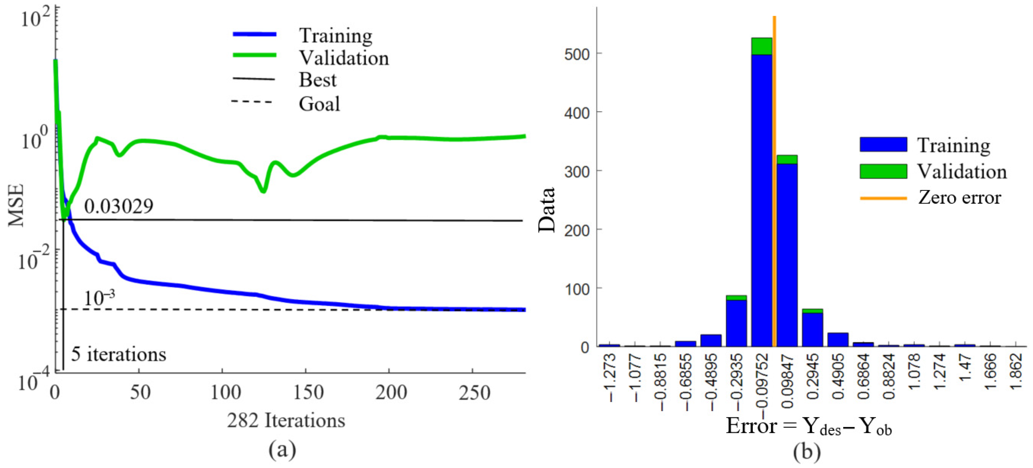
Figure 1. Tomato varieties used in this work.
Agriengineering 07 00130 g001
Figure 2. ANN used in this work.
Agriengineering 07 00130 g002
Figure 3. Illustration of the ANN architecture adopted in this work.
Agriengineering 07 00130 g003
Figure 4. Performance of the ANN during training and validation: (a) mean squared error (MSE) and (b) error histogram comparing predicted (Yob) and target (Ydes) outputs.
Agriengineering 07 00130 g004
Figure 5. Relationship between predicted (Yob) and target (Ydes) outputs: (a) during training using 95% of the dataset, (b) during validation with 5% of the data, and (c) considering the entire dataset (training + validation), (d) first-degree regression for 100% of samples, (e) second-degree regression for 100% of samples, and (f) third-degree regression for 100% of samples.
Agriengineering 07 00130 g005
Figure 6. Comparison of the desired output for all samples with (a) the output obtained from the ANN, (b) the output from the first-degree polynomial regression, (c) the output from the second-degree polynomial regression, and (d) the output from the third-degree polynomial regression.
Agriengineering 07 00130 g006
Figure 7. Obtained versus desired outputs for 100% of samples during training and validation phases for (a) flavonoids (mg of rutin 100 g−1), (b) flavonoids (mg of quercetin 100 g−1), (c) lycopene (mg 100 mL−1), (d) beta-carotene (mg 100 mL−1), (e) anthocyanins (mg 100 g−1), (f) carotenoids (mg 100 g−1), (g) phenolic compounds (mg of gallic acid 100 g−1), (h) DPPH (%), (i) FRAP (mol FESO4 g−1), (j) FRAP (µmol FESO4 kg−1), (k) vitamin C (mg 100 g−1), and (l) ascorbic acid (mg 100 mg−1).
Agriengineering 07 00130 g007
Figure 8. Obtained versus desired outputs for 5% of samples in the validation phase (estimates) for (a) flavonoids (mg of rutin 100 g−1), (b) flavonoids (mg of quercetin 100 g−1), (c) lycopene (mg 100 mL−1), (d) beta-carotene (mg 100 mL−1), (e) anthocyanins (mg 100 g−1), (f) carotenoids (mg 100 g−1), (g) phenolic compounds (mg of acid gallic 100 g−1), (h) DPPH (%), (i) FRAP (mol FESO4 g−1), (j) FRAP (µmol FESO4 kg−1), (k) vitamin C (mg 100 g−1), and (l) ascorbic acid (mg 100 mg−1).
Agriengineering 07 00130 g008
Figure 9. Obtained versus desired outputs for 5% of samples in the validation phase (estimates) for (a) vitamin C (mg 100 g−1) and (b) ascorbic acid (mg 100 mg−1).
Agriengineering 07 00130 g009
Table 1. Comparison between target values (Ydes) and those predicted by the ANN during both training and validation phases.
ANNSpecified ValueAchieved Value
Iterations1000282
Time (s)608
Training performance (MSE)0.0010.000999 *
Training correlation (R2)1.00.9148
Validation performance (MSE)0.0010.03029
Validation correlation (R2)1.00.8609
Best validation performance (iteration)1005
Correlation (R2) of 100% of samples via ANN1.00.9025
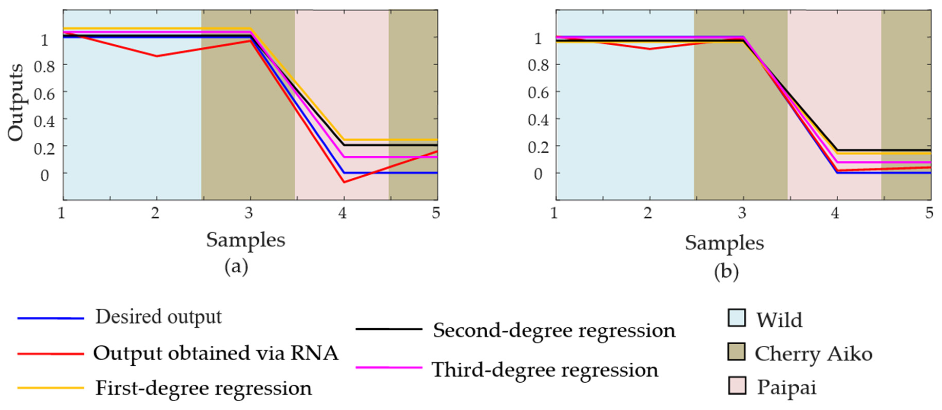
First-degree regression (R2) for 100% of samples1.00.8817
Second-degree regression (R2) for 100% of samples1.00.8819
Third-degree regression (R2) for 100% of samples1.00.8941
* Achieved criterion.
Table 2. Weights W1 represent the connections between the neurons in the input layer and the hidden layer (WRm)—12 rows and 15 columns (12 × 15).
Neurons in the Hidden Layer
Neurons in the input layer m1m2m3m4m5m6m7m8m9m10m11m12m13m14m15
R1−8.5274−6.18991.7758−4.0797−6.81351.92456.0938−0.5554.0853−0.5534−3.22631.59643.19641.4625−3.7006
R22.4851−1.27330.9146−4.5785−5.57166.5616−0.21830.5956−5.38870.072−3.41580.2731.55183.05460.0446
R30.58051.94293.11542.4426−5.14053.24540.5807−0.2981−1.54119.225216.6548−4.4227−0.840−1.6666−2.5458
R4−0.2361−2.2271.1846−3.77931.1519−2.5137−0.67010.16091.121−0.956−2.2151−1.19611.0664−5.36761.7935
R5−2.6401−2.5067−6.7222−7.82299.4098−1.66731.46250.11370.4789−3.7218−6.1581−5.7297−1.3080.85621.0316
R60.76890.38752.2094−0.35191.2378−0.0994−0.2327−0.4243−0.0967−2.4434−0.55362.06082.09214.60.066
R70.1631−0.39662.61018.57672.2655−1.3073−0.0683−0.52330.7072.49671.9221−0.2551−0.6876.1931.1104
R81.02610.1832.322921.09546.2141−1.5754−1.60780.77130.78218.733113.2627−0.24881.40841.46121.1786
R90.3946−2.52087.8396−7.4163−3.627−7.6013−0.919−0.14142.0722−1.2292−2.3102−5.40337.0866−0.30675.1824
R100.13641.0808−4.5368−1.98473.7342.91011.17640.1058−0.21261.78944.90002.8762−3.5091.3923−2.8117
R11−1.34072.1537−3.3648−2.12243.95953.73990.23150.2308−1.79722.26084.35692.8795−4.8801.2431−1.9319
R121.77841.88520.3609−11.2732.5423−2.2087−2.6742−0.78550.2872−0.8562−1.01912.40970.2308−1.88450.1018
Table 3. Weights W2 of the connections between the neurons in the hidden and output layers (Wmi)—15 rows and 12 columns (15 × 12).
Neurons in the Output Layer
Neurons in the hidden layer i1i2i3i4i5i6i7i8i9i10i11i12
m1−1.1279−1.1288−2.7619−2.15480.584−3.0818−1.1356−1.45160.01260.0126−1.1279−1.1288
m22.01952.77050.36744.56350.35717.2269−8.5052−7.61771.0761.0762.01952.7705
m30.42880.41930.0412−0.2552−0.14480.00820.80130.9234−0.0274−0.02740.42880.4193
m40.02830.0510.12830.06320.1161−0.0169−0.00910.00710.00390.00390.02830.051
m5−0.6479−0.6358−0.00110.1510.5050.06040.54120.4067−0.0079−0.0079−0.6479−0.6358
m62.52192.20022.24491.1621−0.49183.19656.09825.8724−0.499−0.4992.52192.2002
m7−0.818−0.6751−3.1964−2.44550.605−3.6152−2.5168−2.81240.08750.0875−0.818−0.6751
m8−2.4192−2.096−6.5673−7.39131.4047−6.2779−2.9087−3.44910.60210.6021−2.4192−2.096
m9−2.7672−1.8849−7.0939−4.05331.6531−2.4244−11.1474−11.10020.5070.507−2.7672−1.8849
m10−0.1757−0.2555−1.3204−0.50410.2582−0.11210.0839−0.05890.02260.0226−0.1757−0.2555
m110.15340.21121.19340.4441−0.35470.1233−0.0750.0521−0.0285−0.02850.15340.2112
m126.16876.13691.24074.4115−2.17530.77790.35610.741−0.4564−0.45646.16876.1369
m131.00691.6743−0.2913.12630.18783.6519−8.8392−8.11340.95860.95861.00691.6743
m140.9440.9111−0.0213−1.39632.2297−0.1665−0.4242−0.4378−0.0927−0.09270.9440.9111
m154.56523.59795.96153.0844−1.3273.051813.542913.0881−0.9047−0.90474.56523.5979
Table 4. Biases b1 and b2 of the neurons in each layer (hidden and output).
Neurons in the Hidden Layer (15 × 1)Neurons in the Output Layer (12 × 1)
11.94151−0.3373
25.6420
3−8.969520.1225
4−16.50843−0.3217
56.68654−0.7471
6−5.37255−0.3581
7−2.259560.0826
84.6028
9−6.142370.9655
10−0.708581.1458
11−2.68919−0.3927
12−11.2968100.2316
137.0877110.1225
14−9.153812−0.3217
154.3167
Disclaimer/Publisher’s Note: The statements, opinions and data contained in all publications are solely those of the individual author(s) and contributor(s) and not of MDPI and/or the editor(s). MDPI and/or the editor(s) disclaim responsibility for any injury to people or property resulting from any ideas, methods, instructions or products referred to in the content.

