Aerodynamic Optimization and Wind Field Characterization of a Quadrotor Fruit-Picking Drone Based on LBM-LES

Abstract

Picking fruits from tall fruit trees manually is laborious and inefficient. Rotary-wing drones, a low-altitude carrier platform, can enhance the picking efficiency for tall fruit trees when combined with picking robotic arms. However, during the operation of rotary-wing drones, the wind field changes dramatically, and the center of gravity of the drone shifts at the moment of picking, leading to poor aerodynamic stability and making it difficult to achieve optimized attitude control. To address the aforementioned issues, this paper constructs a drone and wind field testing platform and employs the Lattice Boltzmann Method and Large Eddy Simulation (LBM-LES) algorithm to solve the high-dynamic, rapidly changing airflow field during the transient picking process of the drone. The aerodynamic structure of the drone is optimized by altering the rotor spacing and duct intake ratio of the harvesting drone. The simulation results indicate that the interaction of airflow between the drone’s rotors significantly affects the stability of the aerodynamic structure. When the rotor spacing is 2.8R and the duct ratio is 1.20, the lift coefficient is increased by 11% compared to the original structure. The test results from the drone and wind field experimental platform show that the rise time ($t_r$) of the drone is shortened by 0.3 s, the maximum peak time ($t_p$) is reduced by 0.35 s, and the adjustment time ($t_s$) is accelerated by 0.4 s. This paper, by studying the transient wind field of the harvesting drone, clarifies the randomness of the transient wind field and its complex vortex structures, optimizes the aerodynamic structure of the harvesting drone, and enhances its aerodynamic stability. The research findings can provide a reference for the aerodynamic optimization of other types of drones.

1. Introduction

Fruit is the third-largest agricultural industry in China, and the development of fruit-picking technology directly affects the benefits of the fruit industry [1,2]. Take lychee, longan, and other tall fruit trees as examples. Since most of their planting areas are in hilly and mountainous regions and the trees are relatively tall, manual picking is very difficult [3,4]. With the continuous innovation and application of robotic technology, the role of fruit-harvesting drones is becoming increasingly important. They can effectively improve the efficiency and quality of fruit picking, reduce labor costs and intensity, and promote the modernization and intelligent development of agricultural production.

Currently, research on picking robots for tall fruit trees such as lychee and longan is relatively scarce [5,6]. The challenges lie in how robots can stably navigate to target points on hilly terrain and how to adjust their height at will for picking operations when facing trees with great height and span [7]. Drones, as low-altitude flying carriers, are not only free from height restrictions for picking but also adaptable to complex mountainous terrain [8,9]. Moreover, due to their high degree of movement freedom, they can quickly and efficiently carry out picking operations after the visual module identifies the picking targets [10]. However, the complex orchard environment requires that the size of the harvesting drone not be too large, while ensuring that it has sufficient lift to carry the weight of the picked fruits [11,12,13]. This means that the harvesting drone must be lightweight, have a large lift, and meet aerodynamic stability characteristics. Therefore, studying the transient wind field of the harvesting drone, solving for the optimal structure of the harvesting drone, and improving its aerodynamic stability during the picking process are of great significance [14,15].

Currently, research on rotor flow fields is primarily divided into two approaches: experimental and theoretical methods. Theoretical studies typically use numerical simulations to explore turbulent motion processes, aiming to reveal the flow characteristics of the downwash airflow and its impact on drone flight [16,17,18]. Computational Fluid Dynamics (CFD) is a numerical simulation method that solves fluid dynamics equations using computers. It can simulate the fluid motion around the rotor, capture vortex flow details, and uncover the characteristics of airflow around the rotor [19,20,21]. Reference [22] employed CFD (The abbreviations are listed in Appendix A) to investigate the distribution characteristics of the downwash flow field during hover of quadrotor agricultural drones. They analyzed the flow phenomena of the downwash airflow across different time and spatial dimensions, revealing the “spiral effect” of the downwash and its impact on agricultural production. Reference [23] used CFD simulations to analyze the wing area and installation angle of a tilt-rotor drone. By adjusting the angle of attack to induce downwash flow separation between rotors, they improved the aerodynamic performance of the harvesting drone. Reference [24] applied the Lattice Boltzmann Method (LBM) for numerical simulation of the downwash airflow field of a hexacopter agricultural drone, studying the airflow separation characteristics and equivalent airflow coverage area under different flight speeds and hover heights. Reference [25] also utilized LBM to simulate the downwash wind field of a hexacopter agricultural drone in flight, investigating the flow field distribution characteristics under various flight parameters. Reference [26] conducted large eddy simulations (LESs) of the downwash airflow for a single-rotor agricultural drones using the LBM method, finding that the asymmetric distribution of the downwash flow during flight might affect the uniformity of droplet distribution. Zhu et al. [27], using CFD, studied the flow characteristics and velocity distribution of quadrotor agricultural drones at different flight speeds, analyzing the impact of vortices generated during flight on the drift of spray droplets. This body of work provides crucial insights into the aerodynamic characteristics and flow field distribution of drones in agricultural applications, contributing to improved drone design and performance in real-world operations.

Wang Chunyang [28] and colleagues from Northwestern Polytechnical University, based on the leaf element momentum theory combined with experimental data, established a coaxial dual-rotor duct aerodynamics model and a thrust duct aerodynamics model. Using the developed models, they performed longitudinal equilibrium solutions and stability analysis for a drone in both hover and transition states. For coaxial multirotor drones, Yoon et al. [29] conducted high-precision numerical simulations, validating that coaxial multirotor drones, when using supercomputing platforms, generate stronger downwash airflow compared to single-axis multirotor drones, thereby increasing the aircraft’s payload capacity and improving hover efficiency. Lei et al. [30] analyzed the downwash flow distribution for both single-axis and coaxial multirotor drones and verified their findings through wind tunnel experiments, concluding that coaxial multirotor drones exhibit more stable structures and stronger resistance to lateral wind disturbances. This research contributes to improving the aerodynamic performance and stability of coaxial multirotor drones, offering insights for future drone design and application in complex environments.

Overall, current research on downwash flow fields, both domestically and internationally, has explored various vortex phenomena such as the spiral effect, ground effect, and horseshoe vortices, and examined their impact on operational performance [31,32,33]. However, most studies on flow fields focus on static processes and their effects on droplet deposition, with limited research on how drone-induced wind fields affect the aerodynamic stability of the drone itself. In this context, we propose a novel simulation method combining the LBM with LES to investigate the transient wind field during the drone’s harvesting process [34,35,36]. Our experiments also demonstrate that this method is capable of solving the transient wind field for drones. The main contributions of this work are as follows:

• A novel approach for studying transient wind fields. We propose a new method for investigating transient wind fields based on LBM-LES. This approach enables more accurate simulation of both large-scale turbulent structures and the microscopic fluid motion, providing improved turbulence information.
• Interaction between drones and tree canopy. By designing a porous medium model to represent the tree canopy surface, we examine the interaction between the harvesting drone and the tree canopy. This interaction is essential for understanding the aerodynamic effects during the harvesting process.
• Experimental validation and aerodynamic optimization. We developed an experimental platform to validate the accuracy of our simulation algorithm. Furthermore, we explored the impact of rotor spacing and duct intake ratio on the drone’s transient wind field and conducted aerodynamic structural optimization for the harvesting drone.

This research contributes to improving the understanding of drone-induced wind fields and their effects on the drone’s aerodynamic stability during harvesting operations, offering new insights for drone design and operational efficiency.

2. Materials and Methods

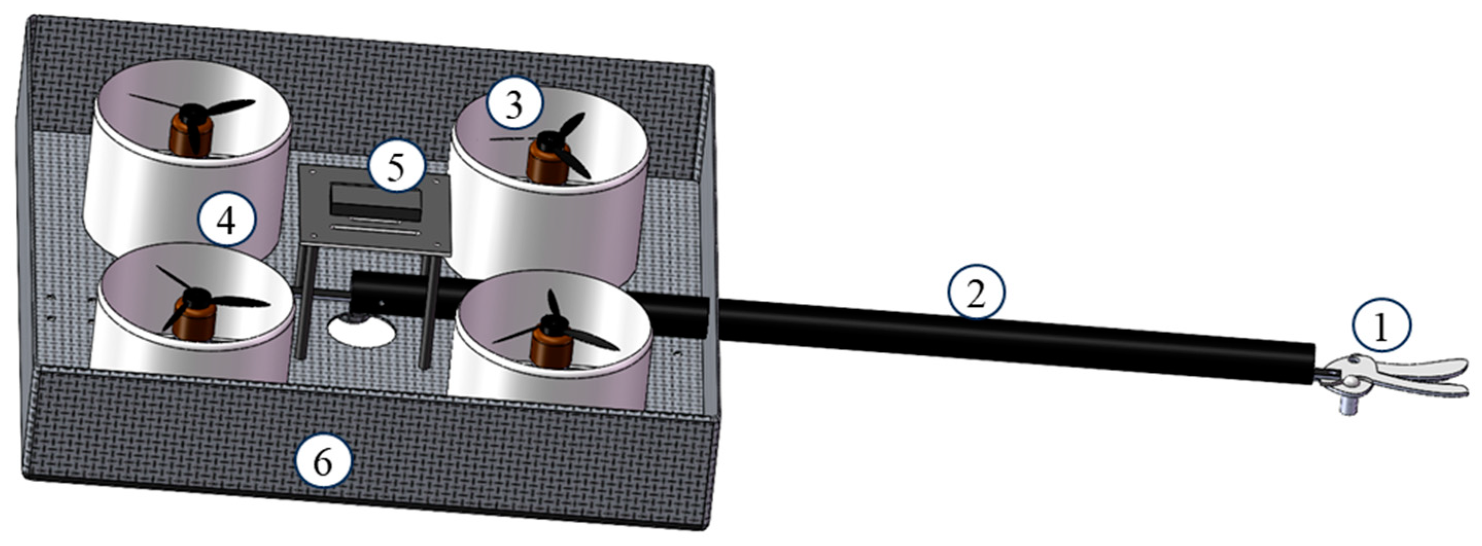
2.1. Establishment of Drone Model

The harvesting drone mentioned in this paper is a self-built quad-rotor ducted drone, with the parameters shown in

Table 1. Harvesting drone parameter table.

Project Parameters	Value
Drone Weight	2.38 kg
Fuselage Length	610 mm
Fuselage Width	670 mm
Harvesting Rod Extension Distance	500 mm
Symmetrical Motor Spacing	595 mm
Number of Rotors	4
Rotor Diameter	337 mm

. The physical models of the harvesting drone’s duct, fuselage shell, and picking rod are modeled and processed according to standard design requirements, which can effectively ensure the precision of the models. The blades are obtained through high-precision 3D scanners to acquire 3D models and then combined with Boolean operations to establish the geometric model of the entire computational domain. Figure 1 shows the actual harvesting drone and the model in the simulation environment.

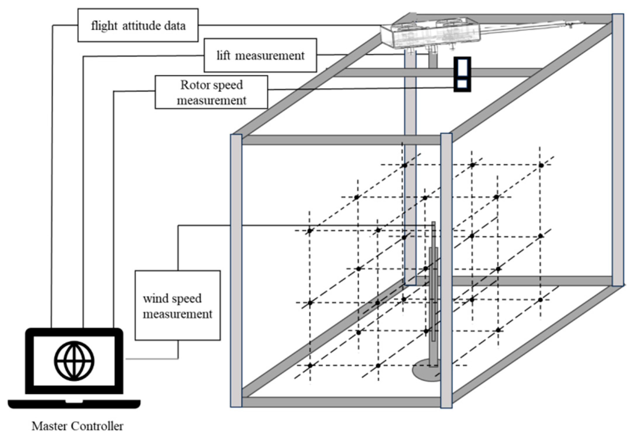
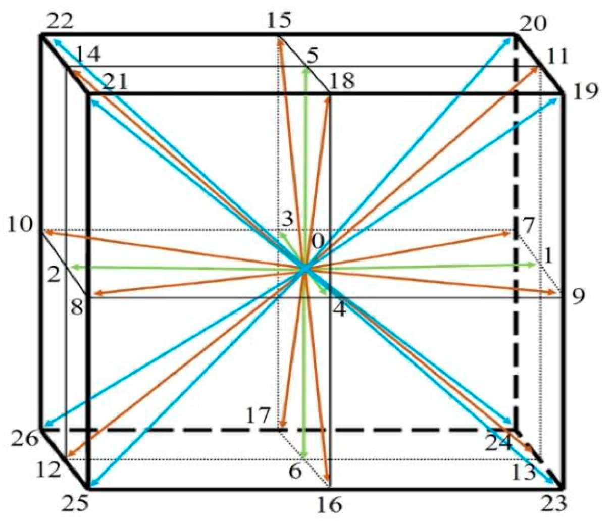
2.2. Establishment of Drone Wind Field Testing Platform

As illustrated in Figure 2, this platform serves as a dedicated testbed for the harvesting drone, aiming to precisely measure rotor speed, variations in the drone’s lift force, and wind field characteristics at designated positions. The central control unit is responsible for acquiring data from the drone’s attitude sensors and transmitting control signals to regulate rotor operation. A tensile sensor is installed at the interface between the drone and the base to assess variations in the lift coefficient. As shown in Figure 2, this platform is specifically designed for wind field testing of the drone, where the dashed framework indicates the sensor measurement locations. A thermosensitive anemometer probe is deployed at these designated points to record wind field parameters and validate the simulated airflow distribution of the harvesting drone. As presented in

Table 2. Fundamental specifications of the sensors.

Measurement Device	Measurement Range	Resolution	Accuracy	Other Specifications
Tensile Sensor	0–10 kg	0.01	0.3%	Combined error: ≤±0.3%; Sensitivity: 1.0/2.0 ± 10% mV/V
Rotational Speed Measurement	2.5–99,999 RPM	0.01	±0.5% + 1	Sampling rate: 0.5 sample/s Testing distance: 50–500 mm
Thermosensitive Anemometer Probe	0.1–30.0 m/s 0–50 °C 0–9999 m3/min	0.01	±0.5% + 1	Measurement area: 0.999 ft2

, the fundamental specifications of the various sensors used in this platform are summarized.

2.3. LES-LBM Numerical Simulation

In computational fluid dynamics (CFD), dynamic grid techniques are commonly used in dynamic simulations to analyze the hydrodynamic characteristics of rotors in high-speed rotational motion. For complex quadrotor models with intricate boundary conditions, mesh reconstruction during the numerical simulation process often consumes significant computational time, and it is prone to generating negative volumes, leading to computational errors. On the other hand, the Lattice Boltzmann Method (LBM) is a mesoscopic-scale computational technique that differs from traditional CFD methods. From a discrete grid perspective, LBM exhibits properties similar to the Euler method; however, from its mesoscopic scale and particle distribution-based statistical approach, it also shares characteristics with the Lagrangian method. LBM offers significant advantages in solving three-dimensional flow field problems involving complex boundary conditions and non-stationary moving objects [37].

In the process of using the Lattice Boltzmann Method (LBM) for simulation and solution, it is necessary to consider the divergence of velocity in space. Therefore, the D3Q27 model is adopted. This model includes 27 discrete velocity directions: One velocity direction represents a fluid particle at rest: (0, 0, 0); six velocity directions correspond to positive and negative velocities along the x, y, and z axes: (±1, 0, 0), (0, ±1, 0), (0, 0, ±1); twelve velocity directions represent velocities along the diagonals of the coordinate plane: (±1, ±1, 0), (±1, 0, ±1), (0, ±1, ±1); eight velocity directions represent velocities along the space diagonals: (±1, ±1, ±1). The model is shown in Figure 3.

In order to better study the complex transient wind field of the harvesting drone, the concept of Large Eddy Simulation (LES) is incorporated into the Lattice Boltzmann Method (LBM). This approach allows for a more accurate simulation of the large-scale structures of turbulence as well as the microscopic motion of fluid, providing more precise turbulence information. Since the LES method primarily analyzes large-scale vortices directly, the effects of small-scale vortices are handled by introducing a subgrid-scale model, with the Smagorinsky model being the most efficient. In the Smagorinsky model, the turbulent viscosity ($v_t$) is calculated using the following relationship:

$$v_t{=(C_s∆)}^2\sqrt{2S_{ij}{S}_{ij}}$$

(1)

$S_{ij }$ represents the components of the strain rate tensor of the fluid, defined as the symmetric part of the velocity gradient. $C_s$ is the Smagorinsky constant, which, due to the lattice size settings in the simulation environment, is set to 0.12 in this study. Δ is the lattice size and is set to 0.0125.

2.4. Simulation Boundary Condition Setting

2.4.1. Simulation Parameter Setting

The fluid analysis type is unidirectional external flow, with a no-flow condition set for the surrounding space. A CFD simulation method based on the Lattice Boltzmann Method (LBM) is used to study the wind field of the fruit-harvesting drone. The parameters for the air are set at 1.225 kg/m³.

In the simulation environment, the three-dimensional coordinate system for the fruit-harvesting drone is set as follows: the Y-axis represents the direction of gravity, the X-axis positive direction is aligned with the direction of the drone’s picking arm (forward direction), and the Z-axis represents the width of the drone. The computational domain has a spatial size of 6 m × 4 m × 6 m. The XOZ plane is set as the ground, with gravity acceleration considered along the Y-axis, and the gravity acceleration is set to −9.8 m∙s⁻². The generation of rotor lift and downwash flow field are the key components of the drone. To accurately capture the airflow field, the lattice resolution around the four rotors is set to 0.025 m, the resolution of the duct is set to 0.1 m, the global spatial discretization resolution of the computational domain is set to 0.2 m, and the resolution of the airflow wake is set to 0.0125 m. The time step is set to 0.015 s, with a total simulation duration of 3 s and a frame rate of 60 Hz.

2.4.2. Boundary Setting for the Interaction Model Between the Drone and the Fruit Trees

Porous Media is a type of solid material that is continuous on a macroscopic scale but contains randomly distributed pore spaces on a microscopic scale. The porous media model is based on the Darcy–Forchheimer law, expressed as:

$$s=-{\displaystyle \frac{\mu }{\alpha }}v-c_2\alpha {\displaystyle \frac{\rho }{2}}|v|v$$

(2)

The momentum loss term is represented as s; $\mu$ is the dynamic viscosity, $\alpha$ is the permeability, 0.395 m²; $\rho$ is the fluid density,1.225 kg/m³; and c₂ is the inertial loss coefficient, 0.4. Based on the fruit tree model, three-dimensional modeling was performed. In the simulation software, the fruit tree model was set as a “Porous Jump”. The “Porous Jump” boundary condition is used to simulate the flow of fluid through a porous medium. This boundary condition is particularly suitable for cases where the thickness of the porous region is small relative to the entire flow domain and where the specific details of the porous structure have minimal impact on the overall flow. It is also applicable in situations where directly simulating the entire porous structure is computationally expensive. By applying the “Porous Jump” boundary condition, the influence of porous media on flow can be approximated without significantly increasing the computational load. The “Porous Jump” boundary condition primarily describes the properties of the porous medium through two parameters. Permeability: Represents the ease with which fluid flows through the porous medium. The higher the permeability, the easier it is for the fluid to pass through. Permeability is generally related to the pore structure of the porous medium. In this experiment, it is set to 0.395. Inertial Loss Coefficient: Reflects the additional pressure loss due to inertial effects when fluid flows through the porous medium. This parameter is related to the fluid’s velocity and accounts for the loss of kinetic energy at higher flow speeds. In this study, it is set to 0.4. As shown in Figure 4, this is the interaction model between the harvesting drone and the fruit trees.

3. Results and Discussion

3.1. Interaction Between the Drone and the Canopy Wind Field at Different Distances

In the investigation of the interaction between the harvesting drone and the fruit tree canopy, it is essential to adjust the distance between the drone and the canopy edge. The distance d is set to −30 cm, 0 cm, and 30 cm. Figure 5a–c illustrate the wind field distributions corresponding to d = −30 cm, 0 cm, and 30 cm, respectively. The results indicate that the interaction between the rotor airflow and the tree canopy is closely related to the foliage density.

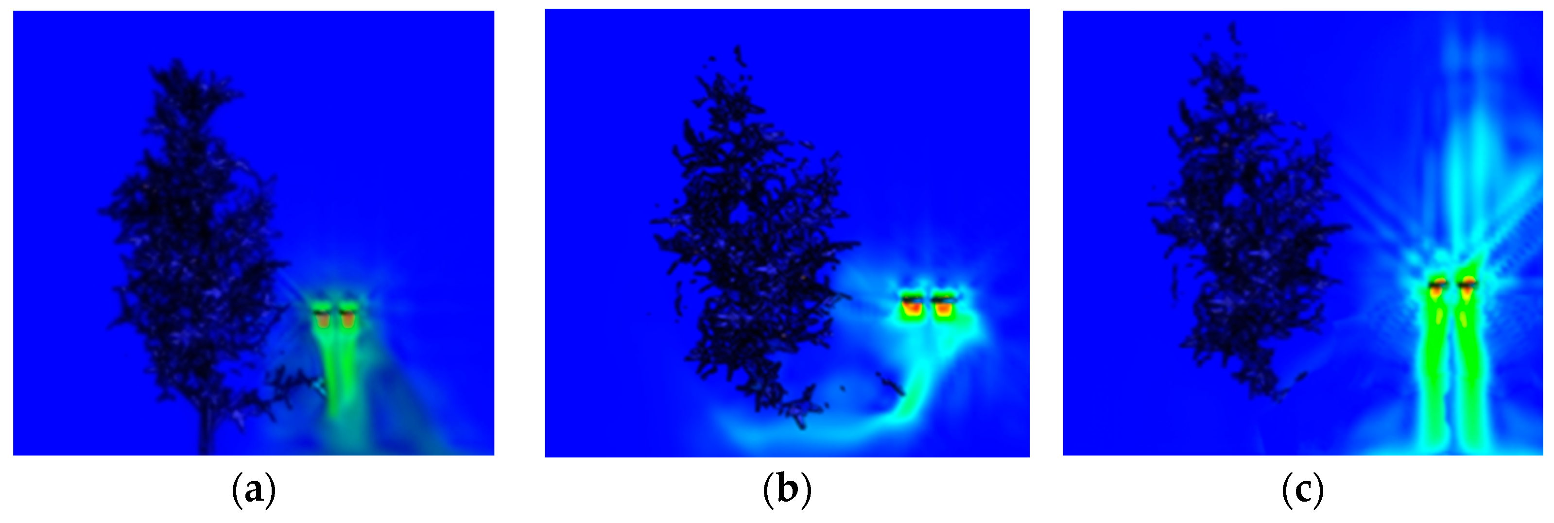
• When d = −30 cm, the foliage density is relatively high, causing the dense canopy to absorb part of the kinetic energy, thereby reducing the effective range of the rotor airflow. This leads to increased power consumption when the drone hovers or operates. At this position, the front downwash airflow column undergoes deformation, causing the rear rotor’s downwash airflow to disperse outward, while the front downwash airflow experiences the greatest energy absorption. Consequently, the drone exhibits poor stability and higher power consumption.
• When d = 0 cm, the foliage density decreases slightly, but at this position, the drone enters the vortex ring state. As the airflow interacts with the tree leaves, micro-scale vortices form within the boundary layer of the leaves, enhancing local turbulence intensity. This results in a reduction in lift force and compromises the drone’s stability, requiring continuous rotor speed adjustments to maintain balance.
• When d = 30 cm, the impact of the rotor airflow on the canopy becomes negligible. At this distance, the interaction between the drone’s rotor wind field and the tree canopy can be disregarded.

Figure 5. (a) Represents the harvesting drone’s body covering the edge of the fruit tree canopy by 30 cm, (b) represents the scenario where the drone’s body is positioned exactly at the edge of the fruit tree canopy, and (c) represents the harvesting drone’s body located 30 cm away from the edge of the fruit tree canopy.

Figure 5. (a) Represents the harvesting drone’s body covering the edge of the fruit tree canopy by 30 cm, (b) represents the scenario where the drone’s body is positioned exactly at the edge of the fruit tree canopy, and (c) represents the harvesting drone’s body located 30 cm away from the edge of the fruit tree canopy.

3.2. Transient Wind Field Simulation Results of the Harvesting Drone

In the previous section, this study investigated the interaction between the rotor-induced wind field of the drone and the fruit tree canopy at different distances. The results demonstrate that the turbulence variations in the downdraft of the rotor wind field are highly correlated with the canopy leaf density. However, given that the designed picking arm in this study is approximately 50 cm in length, the influence of the rotor wind field on the fruit tree canopy is temporarily disregarded. Instead, the focus is placed on analyzing the transient variations in the wind field during the harvesting operation of the drone.

To better understand the transient wind field changes during fruit harvesting, a picking test was conducted on a cluster of fruits using the drone, and the drone’s attitude functions as well as rotor speed data during the harvesting process were recorded. When configuring the boundary conditions in the XFlow 2019 simulation software, it was necessary to incorporate the drone’s attitude functions, rotor speed, and environmental boundary conditions, as previously discussed in Section 2.4. The final simulation results are presented in Figure 6.

Figure 6a represents the wind field of the drone during normal hovering, where the downwash flow column is stable, the diffusion gradient is well-formed, and the aerodynamic performance remains relatively stable. Figure 6b illustrates the moment when the drone is affected by its weight during harvesting, causing the front end to tilt downward. At this point, the drone’s pitch angle is approximately 6°. The downwash column beneath the front rotor begins to bend at a distance of about 1 m, and the downwash column below the rear rotor is deformed at a distance of about 0.3 m. Figure 6c depicts the drone continuing to pitch downward with a pitch angle of about 11°, where a distinct stratification occurs in the airflow behind the rear rotor. Figure 6d shows the drone with a pitch angle of approximately 18°, which is the maximum pitch angle. At this stage, both the front and rear rotor downwash flows break up, but the breakdown of the rear rotor’s downwash is more significant. The downwash flow from the front rotor experiences slight stratification at about 1.5 m. Figure 6e,f represent the process of the drone’s pitch angle decreasing as it starts to ascend, with pitch angles of approximately 14° and 6°, respectively. At this point, there is an interaction between the airflow from the front and rear rotors, but no merging occurs. The airflow from the rear rotor fails to continue to diffuse stably, leading to an intersection of aerodynamic performance. Figure 6g shows the drone at a pitch angle of 0° during the ascent, but the downwash flow has not yet returned to a stable state. The intersection of the downwash airflow leads to increased flow dissipation, resulting in higher energy consumption and poor aerodynamic performance. Figure 6h illustrates the drone with a slight positive pitch angle due to inertia, around 5°. The merging airflow between the rotors continues to diffuse downward, approaching a steady state, and the aerodynamic performance begins to stabilize. Figure 6i represents the drone reaching a horizontal state, where the downwash flow field is well-formed and the aerodynamic conditions are almost stable.

According to the simulation results, during the harvesting process of the drone, the airflow interference between the two rotors causes significant changes in the drone’s wind field. The angle between the airflow streams influences the stable diffusion of the downwash flow. Therefore, the rotor spacing results in mutual interaction between the airflows, which in turn affects the overall aerodynamic performance of the drone.

3.3. Aerodynamic Characteristics of the Drone at Different Rotor Spacings

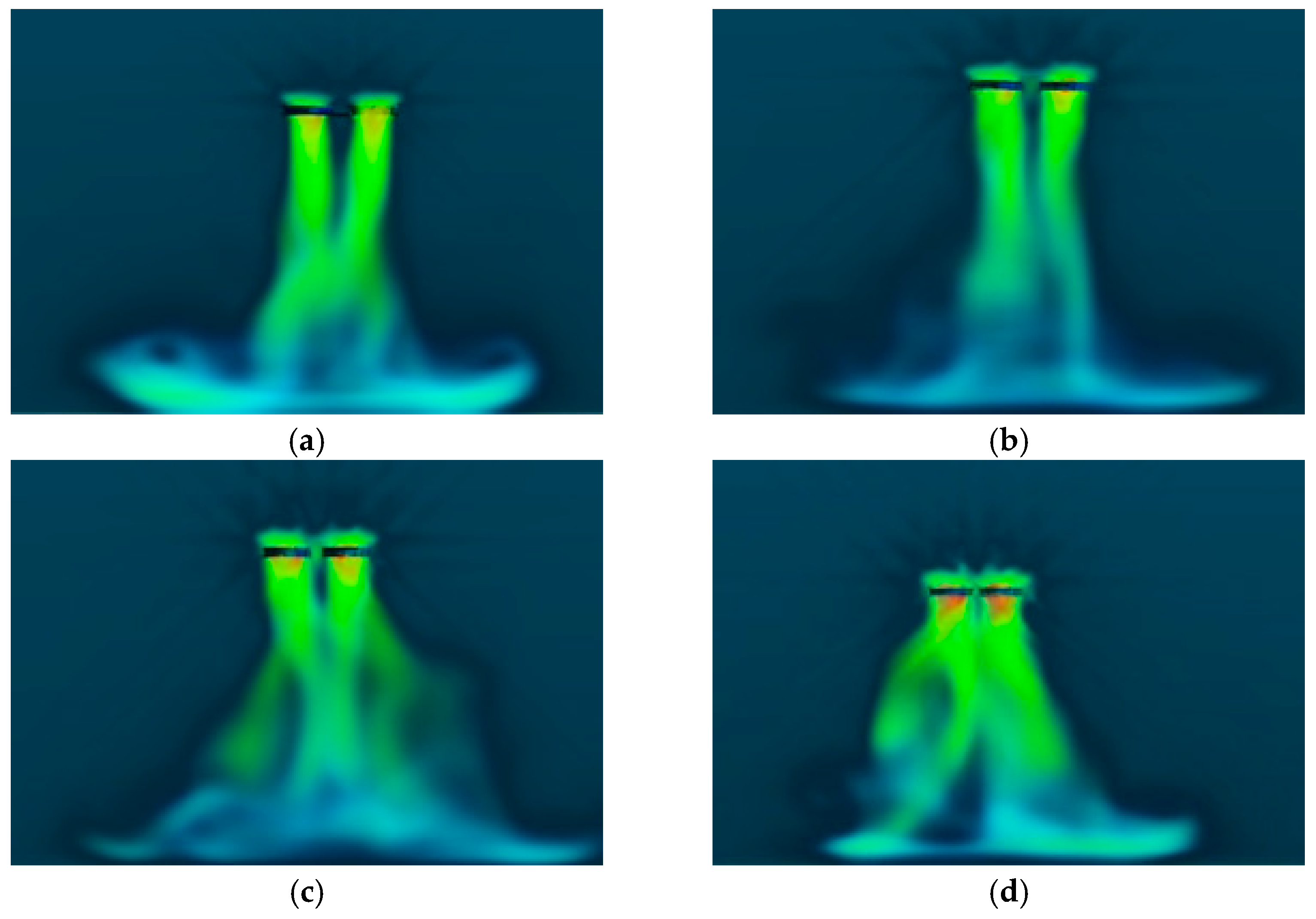
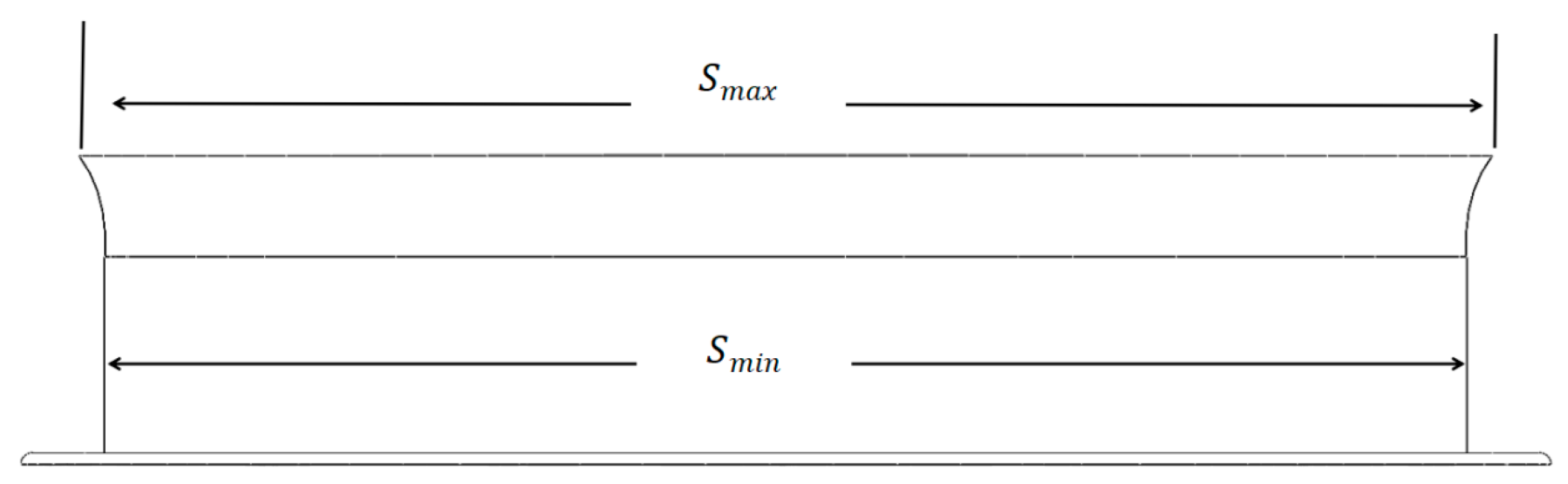
3.3.1. Characteristics of Hovering Downwash Flow Field at Different Rotor Spacings

In the previous section, the transient wind field of the harvesting drone was simulated and solved. Based on the results of the transient simulation, it is necessary to analyze the aerodynamic characteristics of the drone by adjusting the rotor spacing and determining the most suitable rotor spacing for the harvesting drone. Since the wind field in the hovering state significantly influences the aerodynamic stability of the drone, the wind field under hovering conditions is also solved. The rotor speed is set to 6400 rad/s, and considering the operating principle of the quadcopter, the rotor speeds of adjacent rotors are set to be the same in magnitude but opposite in direction. The rotor spacing is set to range from 2.4R to 3.6R, with a variable interval of 0.4R, yielding a total of four groups, where R is the radius of the drone’s rotor.

Figure 7 shows the downwash flow field of the harvesting drone at different rotor spacings. Figure 7a represents the drone with a rotor spacing of 3.6R, where the intersection of the airflow occurs approximately 1.2 m from the drone. At this rotor spacing, the angle between the intersecting airflows is relatively small, resulting in minimal interference between the two rotor airflows. There is no significant interaction between the airflows of the rotors. Figure 7b represents the drone with a rotor spacing of 3.2R, where the intersection of the downwash flows from adjacent rotors occurs approximately 0.8 m from the drone. According to the streamlines, the airflow from the rear rotor is directed vertically downward, causing interference with the airflow from the front rotor. As a result, the merging of the two airflows does not result in effective diffusion, and the aerodynamic effect is suboptimal. Figure 7c represents the drone with a rotor spacing of 2.8R, where the intersection of the downwash flows occurs approximately 0.4 m from the drone. After the downwash flows from the rotors merge, the airflow columns diffuse in a V-shaped pattern. According to the streamline diagram, the airflow is directed vertically downward after the intersection, resulting in an acceleration effect, and subsequently diffuses outward. The airflow field is relatively well-formed, and the aerodynamic performance is stable. Figure 7d shows the drone with a rotor spacing of 2.4R, where the rotor sub-flows begin to intersect approximately 0.1 m below the drone, forming a cylindrical airflow column. The airflow starts to diffuse at a distance of 0.4 m below the drone. However, the premature intersection of the airflows leads to vortex formation, and the airflow at the bottom is not well-formed.

Therefore, based on the analysis of the hovering downwash flow field, the merging effect of the airflows is most positively influenced when the rotor spacing is around 2.8R.

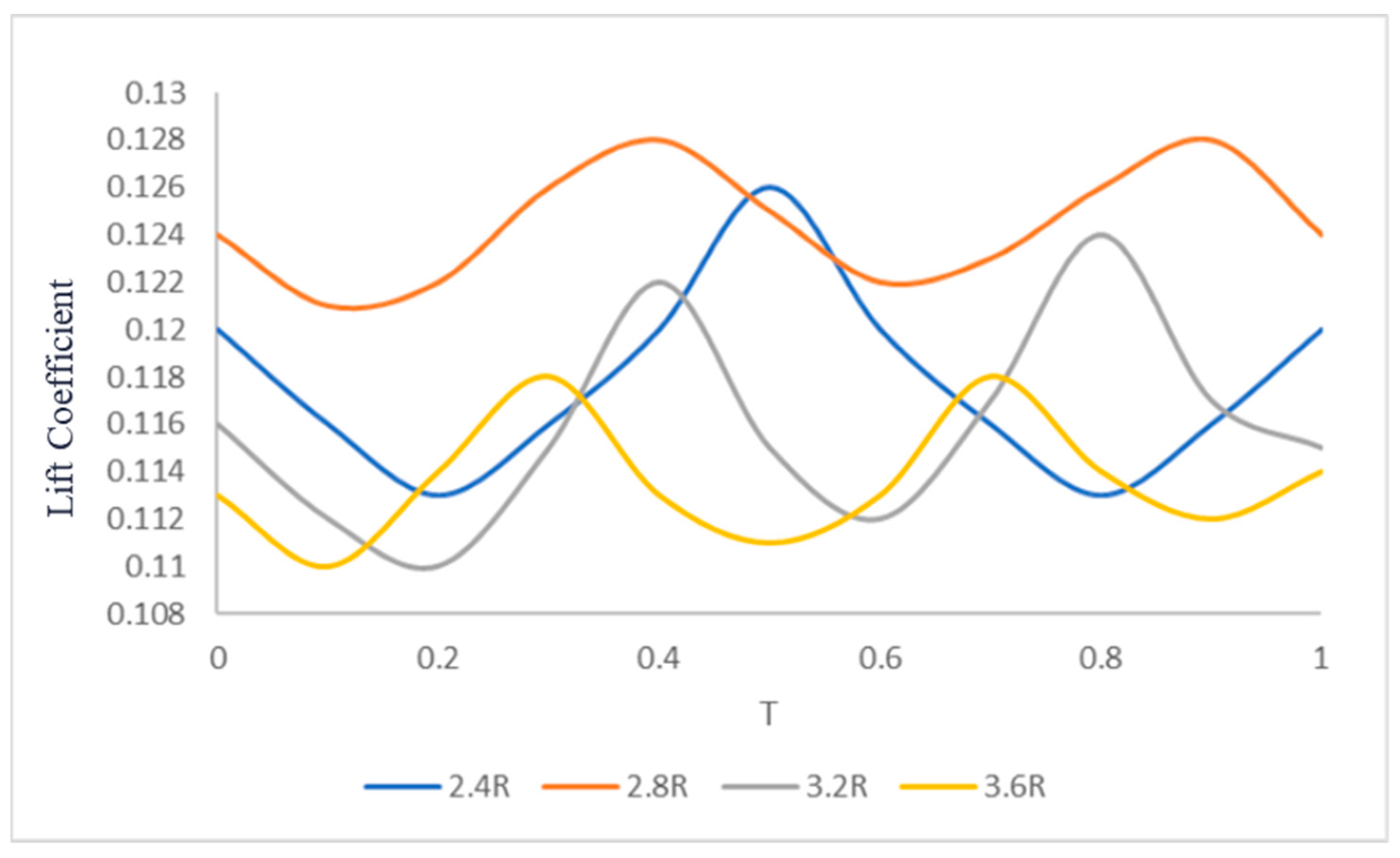
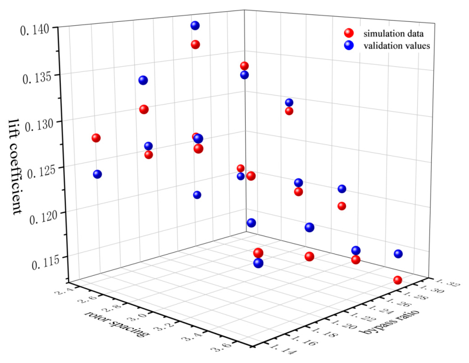
3.3.2. Lift Coefficient at Different Rotor Spacings

The lift coefficient of the drone is an important indicator of its flight efficiency. Therefore, when analyzing the airflow field of the harvesting drone while hovering, the lift coefficient must also be considered as a reference factor.

The lift coefficient of the rotors at different rotor spacings is shown in Figure 8. From a lift perspective, optimal rotor spacing increases the lift coefficient. As the rotor spacing increases from 2.4R to 3.6R, the lift coefficient first increases and then decreases. At a rotor spacing of 2.4R, the interaction between the airflow from adjacent rotors is at its maximum. However, according to the wind field diagram, vortex formation causes dissipation effects, resulting in some loss of kinetic energy, so the lift coefficient is not the highest. When the rotor spacing is 2.8R, the lift coefficient reaches its maximum value. At this spacing, the downwash flows from adjacent rotors exert a positive effect on each other, maintaining the drone’s flow field in a stable state. Additionally, the lift coefficient exhibits relatively small fluctuations, indicating that the drone’s aerodynamic performance is stable at this rotor spacing. As the rotor spacing continues to increase, the lift coefficient decreases, likely because the aerodynamic influence between the rotors becomes weaker, causing the positive effects of flow merging to diminish.

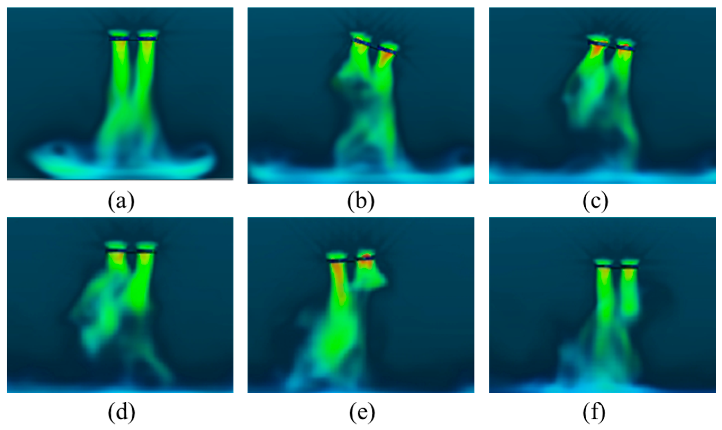
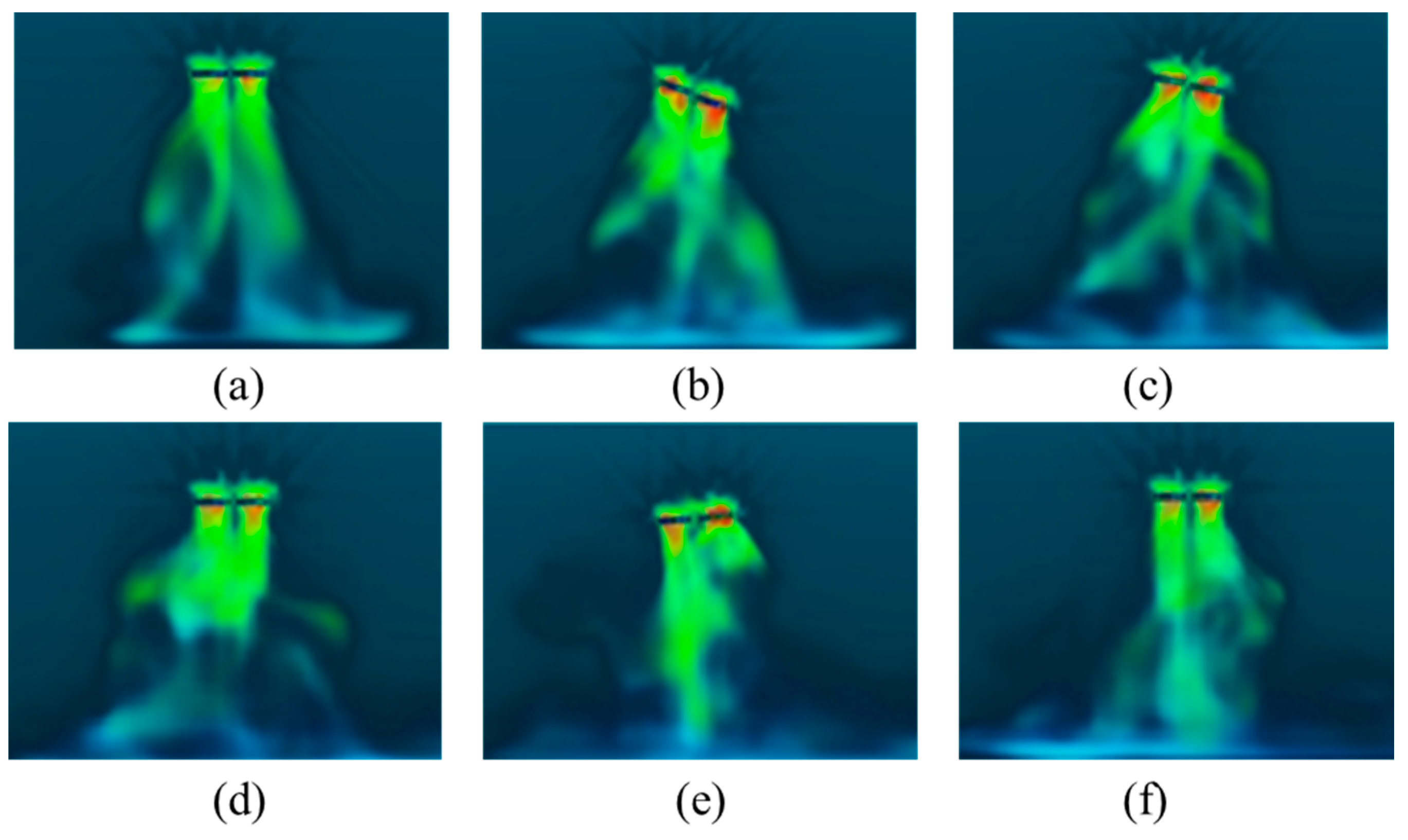
3.3.3. Transient Wind Field Analysis of the Drone at Different Rotor Spacings

The previous two sections studied the flow field characteristics of the harvesting drone during hovering at different rotor spacings. It was found that only at an optimal rotor spacing do the airflows between the rotors merge and accelerate, forming a stable downwash flow that enhances the drone’s stability. An inappropriate rotor spacing, however, can disrupt the aerodynamic stability of the drone, reducing flight efficiency. Therefore, to explore the impact of different rotor spacings on the transient process of the harvesting drone, it is necessary to set up simulations with varying rotor spacings and analyze the transient wind field of the harvesting drone.

To clearly compare the differences in the transient wind field of the harvesting drone at different rotor spacings, the same time points and pitch angles are used as references for each group of figures. Specifically, Figure 9a, Figure 10a and Figure 11a represents the drone in a horizontal state; Figure 9b, Figure 10b and Figure 11b represents the drone with a pitch angle of 18°; Figure 9c, Figure 10c and Figure 11c represents the drone during ascent with a pitch angle of 10°; Figure 9d, Figure 10d and Figure 11d represents the drone after the first ascent to a horizontal state, with a pitch angle of 0°; Figure 9e, Figure 10e and Figure 11e represents the drone continuing to ascend due to inertia, with a pitch angle of 4.5°; and Figure 9f, Figure 10f and Figure 11f represents the drone gradually stabilizing in the horizontal state.

The transient wind fields for the harvesting drone with rotor spacing of 3.6R and 3.2R are shown in Figure 9 and Figure 10, respectively. Analysis of these transient wind field diagrams reveals that, in both cases, a noticeable airflow separation phenomenon occurs when the drone is at its maximum pitch angle. This phenomenon is more pronounced when the rotor spacing is 3.6R compared to 3.2R. The reason for this is that with a rotor spacing of 3.6R, the airflow interference between the rotors is reduced, making the vortex behind the rear rotor more susceptible to disruption. Additionally, analysis of the wind field at 2 s, when the drone is in a horizontal position, shows that the downwash flow recovers more quickly in the 3.2R configuration.

Figure 11 and Figure 12 illustrate the transient wind fields of the harvesting drone with rotor spacings of 2.8R and 2.4R, respectively. Upon analysis, it is observed that when the pitch angle reaches its maximum, neither of these configurations experiences airflow vortex breakdown in the downwash, indicating relatively favorable aerodynamic performance for the drone. Comparing the (e) diagrams of the two configurations, it can be seen that with a rotor spacing of 2.8R, the downwash flow remains relatively stable. This stability results in a quicker recovery of the aerodynamic performance of the drone when it first returns to a horizontal position, as the airflow state with a rotor spacing of 2.8R approaches stability more rapidly.

Therefore, through a comparative analysis of the wind field diagrams from the four sets of figures, it can be concluded that when the rotor spacing of the harvesting drone is 2.8R, the downwash flow during the harvesting process is less prone to disruption, and the aerodynamic performance remains relatively stable. Even after the downwash flow field is disturbed, it is able to recover to a stable state relatively quickly.

3.4. Aerodynamic Characteristics of Harvesting Drone Under Different Duct Ratios

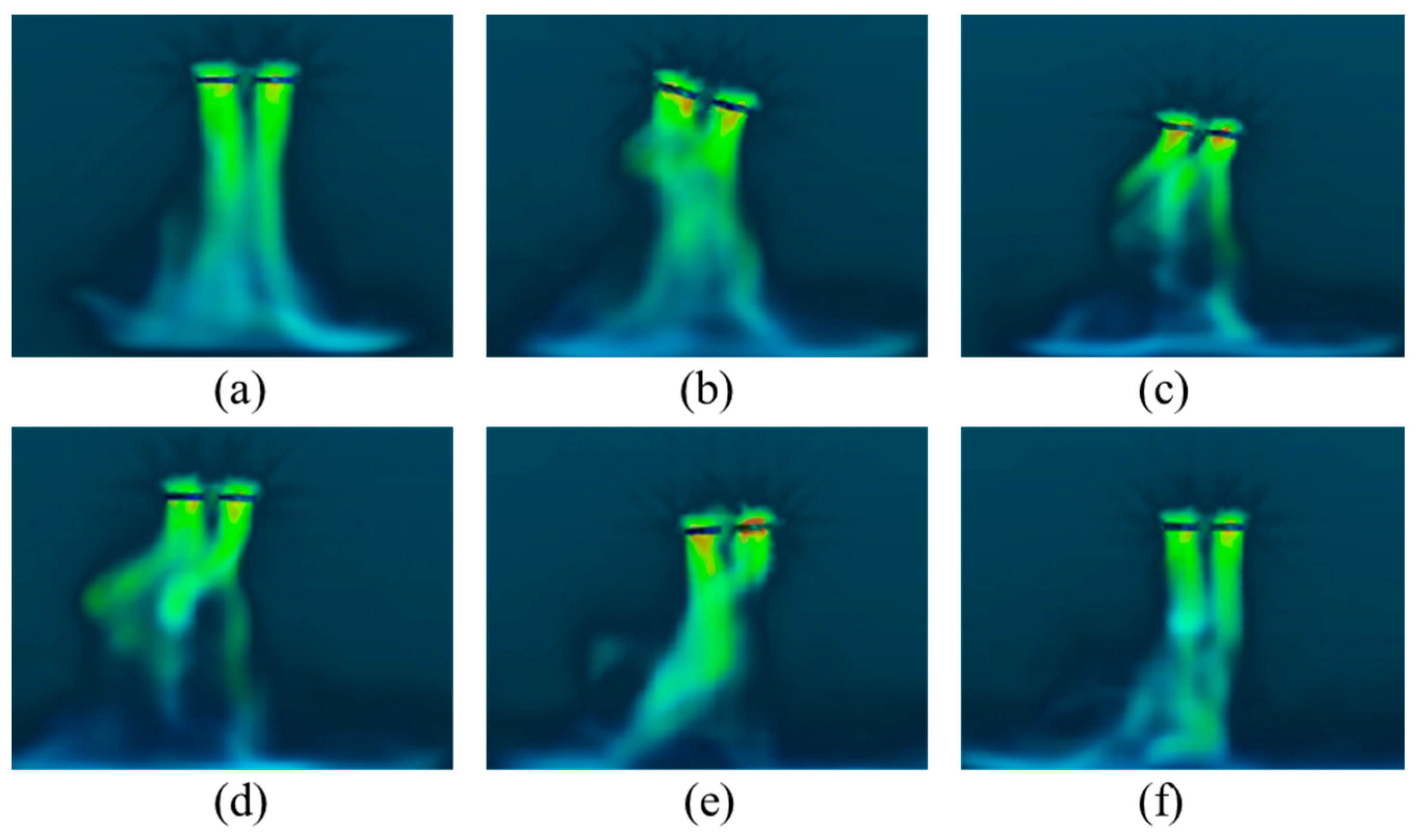
3.4.1. Analysis of Transient Wind Fields in Harvesting Drone at Different Duct Ratios

This study alters the duct compression ratio by changing the ratio of the maximum to the minimum cross-sectional area of the duct. Therefore, the parameter, referred to as the duct ratio β, is defined as the ratio of the maximum to minimum duct area. By varying the value of β, the duct is optimized. The meanings of S_max and S_min within the duct are illustrated in Figure 13.

In order to analyze the aerodynamic characteristics of ducts with different duct ratios, transient wind field simulations were conducted for four different duct ratios. The duct ratios were arranged sequentially from left to right, ensuring that the wind fields of each duct did not interfere with one another. The bypass ratios are sequentially set as $\beta =1.15, \beta =1.20, \beta =1.25, \beta =1.30$. A posture function was then set to simulate the transient wind field of a single duct. As shown in Figure 13, the wind field diagrams for each duct are presented. Specifically, Figure 14a–f correspond to the following time points: 0.8 s, when the duct is in a horizontal position; 1.2 s, with a duct pitch angle of 18°; 1.4 s, with a duct pitch angle of 10°; 1.45 s, with a duct pitch angle of 0°; 1.6 s, with a duct pitch angle of 4.5°; and 2 s, when the duct returns to a horizontal position.

Based on the simulation results, it was found that during hovering, the duct with β = 1.20 exhibits the fastest airflow acceleration and the most concentrated airflow shape, indicating a significant increase in air mass flow rate. During the ascent phase, the airflow within this duct remains stable, and after returning to the horizontal position, its airflow stabilizes most rapidly. Therefore, the duct with β = 1.20 demonstrates the best overall aerodynamic performance.

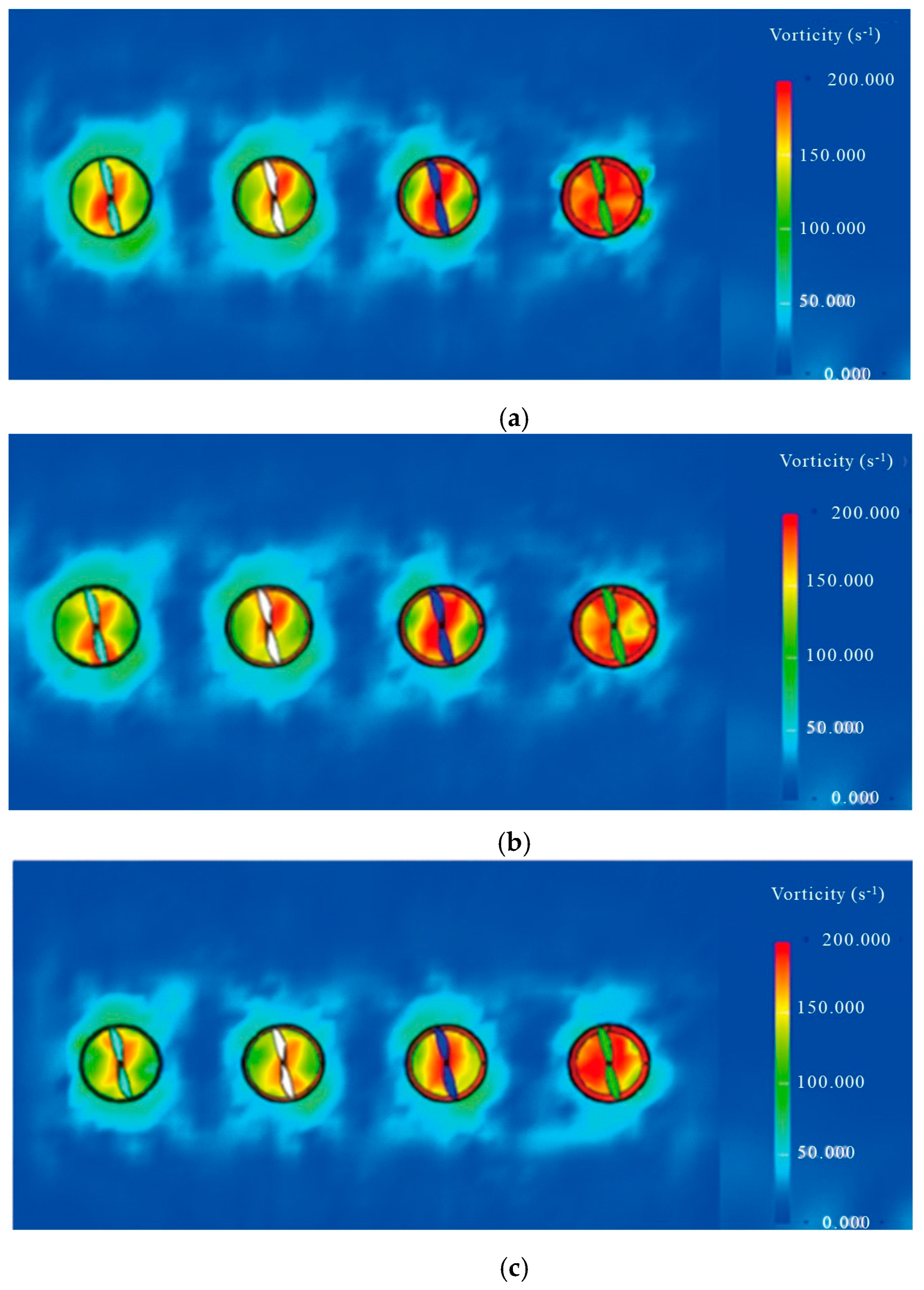
3.4.2. Vorticity Contour Plots of Harvesting Drone Under Different Duct Ratios

The lower the vorticity in the drones, the higher the efficiency of the rotor blades’ work, with less airflow disturbance and dissipation. Figure 15 shows the vorticity contour plots of the rotor blades for the four ducts at 0.8 s, 1.4 s, and 2 s. Based on the analysis of these vorticity contour plots, it can be seen that when β = 1.15 and β = 1.20, the two ducts generate fewer vortices, which provides a greater advantage in improving the aerodynamic stability and reducing dissipation.

3.5. Optimal Structural Configuration of Harvesting Drone

To determine the optimal structural configuration of the harvesting drone, a series of combination experiments were conducted, varying both the duct ratio and rotor spacing. The lift coefficients of the drones were measured for each configuration, and the experimental values were compared with the simulation results.

Through experimental analysis, it was found that the harvesting drone achieves the highest lift coefficient when the rotor spacing is 2.8R and the duct ratio is 1.2. Based on the wind field analysis, it was observed that in this configuration, the flow field around the lower rotor remains relatively stable. Therefore, the rotor spacing of 2.8R and the duct ratio of 1.2 were selected as the optimal structural configuration for the drones. This combination led to an 11% increase in lift coefficient compared to the original structure, thus improving the aerodynamic stability during flight.

Figure 16 shows the experimental lift coefficient values and the corresponding validation results for each configuration.

3.6. Experimental Results Validation

To validate the accuracy of the simulation results, a testing platform for the harvesting drone was designed, and parameters such as wind field velocity and lift coefficient were measured, as shown in Figure 17. Similarly, wind speed sensors were set up in the simulation environment, as explained in Figure 2. Taking the symmetric center point of the UAV as the origin (0, 0, 0), the coordinates of sensor1 are set to (0.2, −0.3, −0.2), and the coordinates of sensor2 are set to (0.2, −0.3, 0). The simulation values at two sensor locations, sensor1 and sensor2, were compared with the experimental values obtained from the harvesting test. The results are shown in Figure 18. It was observed that there was a larger error in wind speed measurements during the drone’s pitching motion, with the worst error reaching approximately 11%, which is within the acceptable experimental error range. The possible cause of this error is that during this phase, the drone’s wind field was in its most unstable state, and the variation was too large to be accurately measured. At other measurement time points, the measurement error for the harvesting drone was approximately 4%. Therefore, it can be concluded that the simulation results for the transient wind field of the harvesting drone are accurate.

Based on the above experimental analysis, it was found that the flow field performance of the drones is relatively better when the rotor spacing is around 2.8R, and the duct ratio design also shows good aerodynamic effects. Therefore, the overall structure of the drones was redesigned accordingly. To demonstrate that the optimized structure can indeed improve the stability of the drones, further orchard harvesting experiments were conducted with the optimized harvesting drone. Finally, the attitude curves before and after the harvesting process were compared, as shown in Figure 19.

Based on the curves in the figure and applying principles from automatic control theory, the time it takes for the harvesting drone to reach a horizontal position is defined as the rise time t_r, which indicates when the drone first reaches a horizontal steady state. The time at which the drone reaches the maximum pitch angle is defined as the peak time t_p, representing the time required for the drone to exceed the horizontal state and reach the first peak during the recovery process. The time when the drone’s pitch angle enters the 1° range is defined as the settling time t_s.

From the comparison between the pre- and post-optimization results, it can be observed that the optimized drone has a rise time t_r that is approximately 0.3 s faster, a peak time t_p that is about 0.35 s faster, and a settling time t_s that is around 0.4 s faster. This indicates that the optimized structure allows the drones to achieve equilibrium more quickly.

4. Conclusions

In this study, a three-dimensional model of the harvesting drone was established, and the LES-LBM method was employed to accurately simulate the transient wind field during the harvesting process. The research focused on both the interaction between the rotor wind field and the fruit tree canopy, as well as the transient wind field variations during harvesting. Additionally, a dedicated drone harvesting test platform was designed and constructed to obtain key parameters such as the drone’s attitude functions, lift force, wind field distribution, and rotor speed, thereby validating the accuracy of the simulation results. The main conclusions are as follows:

• The interaction between the harvesting drone and the fruit tree canopy is primarily influenced by the density of the foliage. When the foliage density is high, a significant portion of the airflow energy is dissipated, leading to increased power consumption and reduced flight stability. Upon initial contact between the rotor airflow and the canopy, microscale vortices in the boundary layer intensify local turbulence, causing a reduction in lift force and a degradation of drone stability. However, when the distance between the drone rotor and the canopy exceeds 30 cm, the interaction effect weakens, and the drone maintains better aerodynamic performance.
• Through LES-LBM simulations, it was observed that the transient wind field undergoes significant variations during the harvesting process. However, after the front and rear rotor airflows merge, the downwash flow stabilizes more rapidly. This suggests that adjusting the rotor spacing could enhance the aerodynamic stability of the harvesting drone. The simulation results indicate that when the rotor spacing is set to 2.8R, transient airflow diffusion is minimized, and the wind field stabilizes more efficiently. Furthermore, a comparison of lift coefficients under different rotor spacings revealed that at a rotor spacing of 2.8R, the periodic lift coefficient increases significantly, improving the overall aerodynamic performance of the drone.
• To further improve the aerodynamic stability of the harvesting drone, an optimized ducted rotor design was proposed by adjusting the duct ratio. Simulation experiments demonstrated that when the β = 1.20, the airflow acceleration effect is most pronounced, and the airflow remains more concentrated, indicating that this duct design effectively enhances airflow velocity. Additionally, during the recovery phase, the optimized duct exhibited better airflow retention, and after the drone returned to a horizontal state, the airflow stabilized more rapidly.
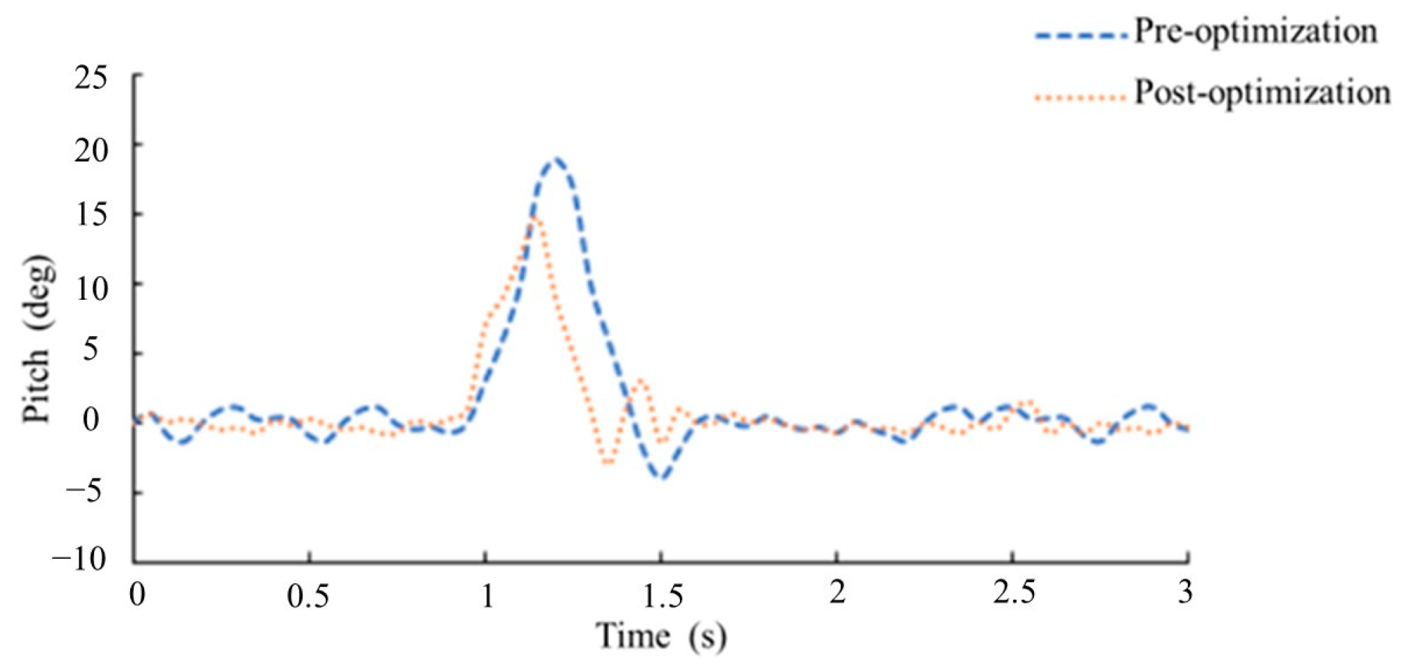
• Based on the optimal rotor spacing and duct ratio, the harvesting drone was reconstructed accordingly. Experimental validation using the harvesting test platform was conducted to compare the attitude function variations before and after optimization. The results showed that the optimized drone achieved a stable horizontal position 0.3 s faster, reduced the maximum pitch angle by 4°, and shortened the adjustment time by 0.4 s. These improvements indicate that the optimized drone can achieve stability more quickly, enhancing operational efficiency and flight performance.

This study provides valuable insights into the structural optimization and aerodynamic enhancement of harvesting drones, laying a foundation for their future applications in precision agricultural operations.

References

1. Chen, H.; Lan, Y.; Fritz, B.K.; Hoffmann, W.C.; Liu, S. Review of agricultural spraying technologies for plant protection using unmanned aerial vehicle (UAV). Int. J. Agric. Biol. Eng. 2021, 14, 38–49. [Google Scholar] [CrossRef]
2. Yang, S.; Tang, Q.; Zheng, Y.; Liu, X.; Chen, J.; Li, X. Model migration for CFD and verification of a six-rotor UAV downwash. Int. J. Agric. Biol. Eng. 2020, 13, 10–18. [Google Scholar] [CrossRef]
3. Carreño, R.M.; Scanavino, M.; D’Ambrosio, D.; Guglieri, G.; Vilardi, A. Experimental and numerical analysis of hovering multicopter performance in low-Reynolds number conditions. Aerosp. Sci. Technol 2022, 128, 107777. [Google Scholar] [CrossRef]
4. Zhang, H.; Qi, L.; Wu, Y.; Musiu, E.M.; Cheng, Z.; Wang, P. Numerical simulation of airflow field from a six–rotor plant protection drone using lattice Boltzmann method. Biosyst. Eng 2020, 197, 336–351. [Google Scholar] [CrossRef]
5. Wang, G.; Han, Y.; Li, X.; Andaloro, J.; Chen, P.; Hoffmann, W.C.; Han, X.; Chen, S.; Lan, Y. Field evaluation of spray drift and environmental impact using an agricultural unmanned aerial vehicle (UAV) sprayer. Sci. Total Environ. 2020, 737, 139793. [Google Scholar] [CrossRef]
6. Guo, Q.W.; Zhu, Y.Z.; Tang, Y.; Hou, C.; He, Y.; Zhuang, J.; Zheng, Y.; Luo, S. CFD simulation and experimental verification of the spatial and temporal distributions of the downwash airflow of a quad-rotor agricultural UAV in hover. Comput. Electron. Agric. 2020, 172, 105343. [Google Scholar] [CrossRef]
7. Wang, L.; Xu, M.; Hou, Q.; Wang, Z.; Lan, Y.; Wang, S. Numerical verification on influence of multi-feature parameters to the downwash airflow field and operation effect of a six-rotor agricultural UAV in flight. Comput. Electron. Agric. 2021, 190, 106425. [Google Scholar] [CrossRef]
8. Shi, Q.; Liu, D.; Mao, H.; Shen, B.; Li, M. Wind-induced response of rice under the action of the downwash flow field of a multi-rotor UAV. Biosyst. Eng. 2021, 203, 60–69. [Google Scholar] [CrossRef]
9. Tang, Q.; Zhang, R.; Chen, L.; Xu, G.; Deng, W.; Ding, C.; Xu, M.; Yi, T.; Wen, Y.; Li, L. High-accuracy, high-resolution downwash flow field measurements of an unmanned helicopter for precision agriculture. Comput. Electron. Agric. 2020, 173, 105390. [Google Scholar] [CrossRef]
10. Zhu, Y.; Guo, Q.; Tang, Y.; Zhu, X.; He, Y.; Huang, H.; Luo, S. CFD simulation and measurement of the downwash airflow of a quadrotor plant protection UAV during operation. Comput. Electron. Agric. 2022, 201, 107286. [Google Scholar] [CrossRef]
11. Lei, Y.; Lin, R. Effect of wind disturbance on the aerodynamic performance of coaxial rotors during hovering. Meas. Control 2019, 52, 665–674. [Google Scholar] [CrossRef]
12. Yao, L.; Wang, Q.; Yang, J.; Zhang, H.; Li, X.; Zhou, Y. UAV-Borne dual-band sensor method for monitoring physiological crop status. Sensors 2019, 19, 816. [Google Scholar] [CrossRef] [PubMed]
13. Chang, K.; Chen, S.; Wang, M.; Liao, J.; Liu, J.; Lan, Y. Numerical Simulation and Experimental Verification of Rotor Airflow Field Based on Finite Volume Method and Lattice Boltzmann Method. Drones 2024, 8, 612. [Google Scholar] [CrossRef]
14. Tang, Q.; Chen, L.P.; Zhang, R.R.; Xu, G.; Deng, W.; Ding, C. Effects of application height and crosswind on the crop spraying performance of unmanned helicopters. Comput. Electron. Agric. 2021, 181, 105961. [Google Scholar] [CrossRef]
15. Zhan, Y.; Chen, P.; Xu, W.; Liu, X.; Li, X.; Wang, Z. Influence of the downwash airflow distribution characteristics of a plant protection UAV on spray deposit distribution. Biosyst. Eng. 2022, 216, 32–45. [Google Scholar]
16. Zhang, H.; Qi, L.; Wan, J.; Cheng, Z.; Wang, P.; Li, X. Numerical simulation of downwash airflow distribution inside tree canopies of an apple orchard from a multirotor unmanned aerial vehicle (UAV) sprayer. Comput. Electron. Agric. 2022, 195, 106817. [Google Scholar]
17. Haddadi, S.; Zarafshan, P.; Dehghani, M. A coaxial quadrotor flying robot: Design, analysis and control implementation. Aerosp. Sci. Technol. 2022, 120, 107260. [Google Scholar] [CrossRef]
18. Del Cerro, J.; Cruz Ulloa, C.; Barrientos, A.; de León Rivas, J. Unmanned Aerial Vehicles in Agriculture: A Survey. Agronomy 2021, 11, 203. [Google Scholar] [CrossRef]
19. Li, J.; Shi, Y.; Lan, Y.; Guo, S. Vertical distribution and vortex structure of rotor wind field under the influence of rice canopy. Comput. Electron. Agric. 2019, 159, 140–146. [Google Scholar] [CrossRef]
20. Hu, H.; Yang, Y.; Liu, Y.; Liu, X.; Wang, Y. Aerodynamic and aeroacoustic investigations of multi-copter rotors with leading edge serrations during forward flight. Aerosp. Sci. Technol. 2021, 112, 106669. [Google Scholar]
21. Tang, D.; Tang, B.; Shen, W.; Zhu, K.; Quan, Q.; Deng, Z. On genetic algorithm and artificial neural network combined optimization for a Mars rotorcraft blade. Acta Astronaut. 2023, 203, 78–87. [Google Scholar]
22. Zhang, Z.; Ma, H. Application of Phase-Locked PIV Technique to the Measurements of Flow Field in a Turbine Stage. J. Therm. Sci. 2020, 29, 784–792. [Google Scholar]
23. Tanabe, Y.; Sugawara, H.; Sunada, S.; Yonezawa, K.; Tokutake, H. Quadrotor Drone Hovering in Ground Effect. J. Robot. Mechatron 2021, 33, 339–347. [Google Scholar]
24. Chatila, J.G.; Danageuzian, H.R. PIV and CFD investigation of paddle flocculation hydrodynamics at low rotational speeds. Sci. Rep. 2022, 12, 19742. [Google Scholar]
25. Li, Y.; Yonezawa, K.; Liu, H. Effect of Ducted Multi-Propeller Configuration on Aerodynamic Performance in Quadrotor Drone. Drones 2021, 5, 101. [Google Scholar] [CrossRef]
26. Kostic, I.; Tanovic, D.; Kostic, O.; Abubaker, A.A.I.; Simonovic, A. Initial development of tandem wing UAV aerodynamic configuration. Aircr. Eng. Aerosp. Technol. 2023, 95, 431–441. [Google Scholar]
27. Cipolla, V.; Dine, A.; Viti, A.; Binante, V. MDAO and Aeroelastic Analyses of Small Solar-Powered UAVs with Box-Wing and Tandem-Wing Architectures. Aerospace 2023, 10, 105. [Google Scholar] [CrossRef]
28. Zhang, Q.; Xue, R.; Li, H. Aerodynamic Exploration for Tandem Wings with Smooth or Corrugated Surfaces at Low Reynolds Number. Aerospace 2023, 10, 427. [Google Scholar] [CrossRef]
29. Ventura Diaz, P.; Yoon, S. High-Fidelity Simulations of a Quadrotor Vehicle for Urban Air Mobility. In Proceedings of the AIAA SCITECH 2022 Forum, San Diego, CA, USA, 3–7 January 2022. [Google Scholar]
30. Chen, Q.; Zhang, J.; Zhang, C.; Zhou, H.; Jiang, X.; Yang, F.; Wang, Y. CFD Analysis and RBFNN-Based Optimization of Spraying System for a Six-Rotor Unmanned Aerial Vehicle (UAV) Sprayer. Crop Prot. 2023, 174, 106433. [Google Scholar]
31. Wang, H.P.; Sun, W.H.; Zhao, C.L.; Zhang, S.J.; Han, J.D. Dynamic Modeling and Control for Tilt-Rotor UAV Based on 3D Flow Field Transient CFD. Drones 2022, 6, 338. [Google Scholar] [CrossRef]
32. Paz, C.; Suárez, E.P.; Gil, C.; Vence, J. Assessment of the Methodology for the CFD Simulation of The Flight of a Quadcopter UAV. J. Wind Eng. Ind. Aerodyn. 2021, 218, 104776. [Google Scholar] [CrossRef]
33. Abichandani, P.; Lobo, D.; Ford, G.; Bucci, D.; Kam, M. Wind Measurement and Simulation Techniques in Multi-Rotor Small Unmanned Aerial Vehicles. IEEE Access 2020, 8, 54910–54927. [Google Scholar]
34. Chen, P.; Douzals, J.P.; Lan, Y.; Cotteux, E.; Delpuech, X.; Pouxviel, G.; Zhan, Y. Characteristics of unmanned aerial spraying systems and related spray drift: A review. Front. Plant Sci. 2022, 13, 870956. [Google Scholar]
35. Ni, M.; Wang, H.J.; Liu, X.D.; Liao, Y.L.; Fu, L.; Wu, Q.Q.; Mu, J.; Chen, X.Y.; Li, J. Design of Variable Spray System for Plant Protection UAV Based on CFD Simulation and Regression Analysis. Sensors 2021, 21, 638. [Google Scholar] [CrossRef] [PubMed]
36. Mohebbi, M.; Rezvani, M.A. Analysis of the effects of lateral wind on a high speed train on a double routed railway track with porous shelters. J. Wind. Eng. Ind. Aerodyn. 2019, 184, 116–127. [Google Scholar] [CrossRef]
37. Dbouk, T.; Drikakis, D. Quadcopter Drones Swarm Aeroacoustics. Phys. Fluids 2021, 33, 057112. [Google Scholar]
Figure 1. Diagram of the harvesting drone. ① Shears Head; ② Harvesting Rod; ③ Rotor Blades; ④ Ducted Fan; ⑤ Flight Controller; ⑥ Fuselage.
Agriengineering 07 00100 g001
Figure 2. Drones wind field testing platform.
Agriengineering 07 00100 g002
Figure 3. The D3Q27 model of the Lattice Boltzmann Method (LBM) consists of 27 discrete velocity directions in a three-dimensional space.
Agriengineering 07 00100 g003
Figure 4. Interaction model between the harvesting drone and the fruit trees.
Agriengineering 07 00100 g004