Simulation Analysis of Energy Inputs Required by Agricultural Machines to Perform Field Operations

Abstract

The evaluation of direct energy inputs and the assessment of the carbon footprint of an agricultural tractor during the execution of an agricultural operation is a complex task. Methodological approaches such as field surveys and life cycle assessments can provide unreliable and non-repeatable results. This study exploits the use of numerical simulation to assess the fuel consumption of two agricultural tractors and their CO₂ emissions during the execution of pesticide treatment and milling. The digital models of the Landini REX 4-120 GB and the Fendt 942 Vario were developed, starting from experimental data acquired during field tests in which the power required at the power take-off (PTO) by the respective operating machine was measured. Two custom working cycles, simulating the two agricultural operations, have been defined and simulated. The estimated fuel consumption was 7.8 L∙ha⁻¹ and 23.2 L∙ha⁻¹, respectively, for the Landini REX 4-120 GB during pesticide treatment and for the Fendt 942 Vario during milling. The corresponding direct energy inputs required for the two agricultural operations were equal to 300.3 MJ∙ha⁻¹ and 893.2 MJ∙ha⁻¹, respectively. The estimated carbon footprint was 26.5 kg_CO2∙ha⁻¹ and 68.4 kg_CO2∙ha⁻¹ for pesticide treatment and for milling, respectively. Moreover, considering the operational efficiency of the systems, an analysis of the available mechanical work supplied by the fuel was conducted.

1. Introduction

The energy inputs required for executing an agricultural operation can be classified based on their direct and indirect source. Direct energy inputs are related to energy resources directly employed for performing agricultural operations and crop production, while indirect energy inputs are dissipated in manufacturing, storage, distribution, and other processes [1,2]. Direct energy inputs strictly depend on the agricultural operations (seeding, milling, spraying) performed and are affected by several factors, including working speed and environmental conditions such as the type of soil, season, and weather [3]. It is well-known that energy obtained from fossil fuels dominates the agricultural sector [4]. Indeed, diesel use is one of the most significant energy inputs, representing 31% of the total [5,6]. Fuel consumption strongly depends on the employed agricultural tractor, the working point of the internal combustion engine (ICE), the performed operation, and the workload. Fuel can be expressed considering its gross calorific value (GCV) or its embodied energy [7,8]. Considering fuel in terms of GCV, diesel’s energetic value is approximatively equal to 45.7 MJ∙kg⁻¹ (or 38.5 MJ∙L⁻¹) [9]. The use of the GCV is justified if the objective is to measure the engine consumption during the execution of a field operation [10,11]. A tractor’s fuel consumption is typically measured in L∙h⁻¹ or L∙ha⁻¹. When it is expressed in L∙ha⁻¹, the working width of the agricultural machinery must be considered. It is important to highlight that not all energy supplied by fuel is converted into useful mechanical work due to losses related to engine efficiency, heat, friction, transmission, and the tractor–implement connection [12].

A tractor’s exhaust emissions are strictly related to fuel consumption. The total amount of greenhouse gases (GHGs) emitted by a system is referred to as the carbon footprint and is often expressed as the amount of emitted carbon dioxide (CO₂) [13]. On average, one liter of burning diesel emits between 2.7 kg and 3.5 kg of CO₂ [14].

Several approaches, including field surveys, reference databases, and life cycle assessments, have been exploited to assess the direct energy inputs required by agricultural machinery during the execution of agricultural operations; however, these methodologies give subjective and unreliable results [15,16]. Moreover, usually for assessing fuel consumption and CO₂ emissions, some expensive, time-consuming, and polluting field tests are required [17].

In this context, simulation tools can be used to develop digital models of tractors, as well as accurately predict the required direct energy inputs and the generated carbon footprint during the execution of agricultural operations. Unfortunately, the use of simulation software is currently exclusively found in the automotive sector. A simulation tool ensures the following advantages [18]: (i) virtually testing different configurations and working scenarios; (ii) easy calculation of the performance of a tractor; (iii) assessing the environmental impact of the execution of an agricultural operation; and (iv) avoiding costly field tests.

The objective of this study is the use of numerical simulations for the estimation of the fuel consumption of two agricultural tractors and their respective carbon footprints during two field operations: (i) pesticide treatment and (ii) milling. The digital models of the tractors have been developed by exploiting experimental data acquired during field tests, in which the power required at the power take-off (PTO) by the respective operating machine (an air-assisted sprayer machine and a milling machine) has been measured. Two different tractors have been modeled, a 77 kW tractor for the pesticide treatment and a 261 kW tractor for milling. For modeling the configurations used during field tests (tractor–sprayer machine and tractor–milling machine), the authors have appropriately adapted the “Autonomie 2023” simulation software that is usually employed in the automotive sector. Two custom working cycles have been defined to simulate the two agricultural operations considered.

The novelty of this work lies in the methodology that has been studied and applied to exploit simulation software to create digital models of tractors and, simulating the execution of agricultural operations, estimate the required direct energy inputs and the generated carbon footprint.

2. Materials and Methods

2.1. Field Tests

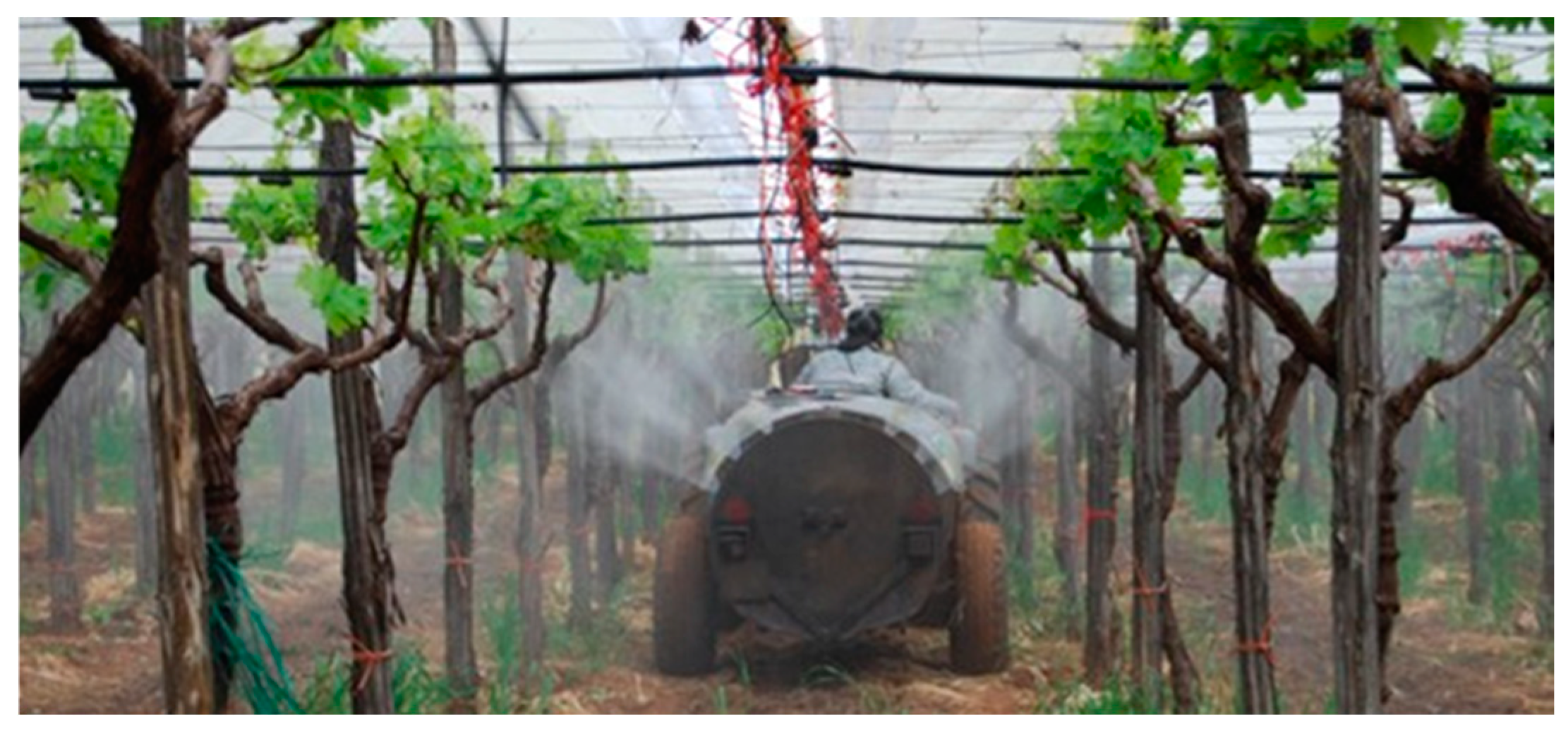
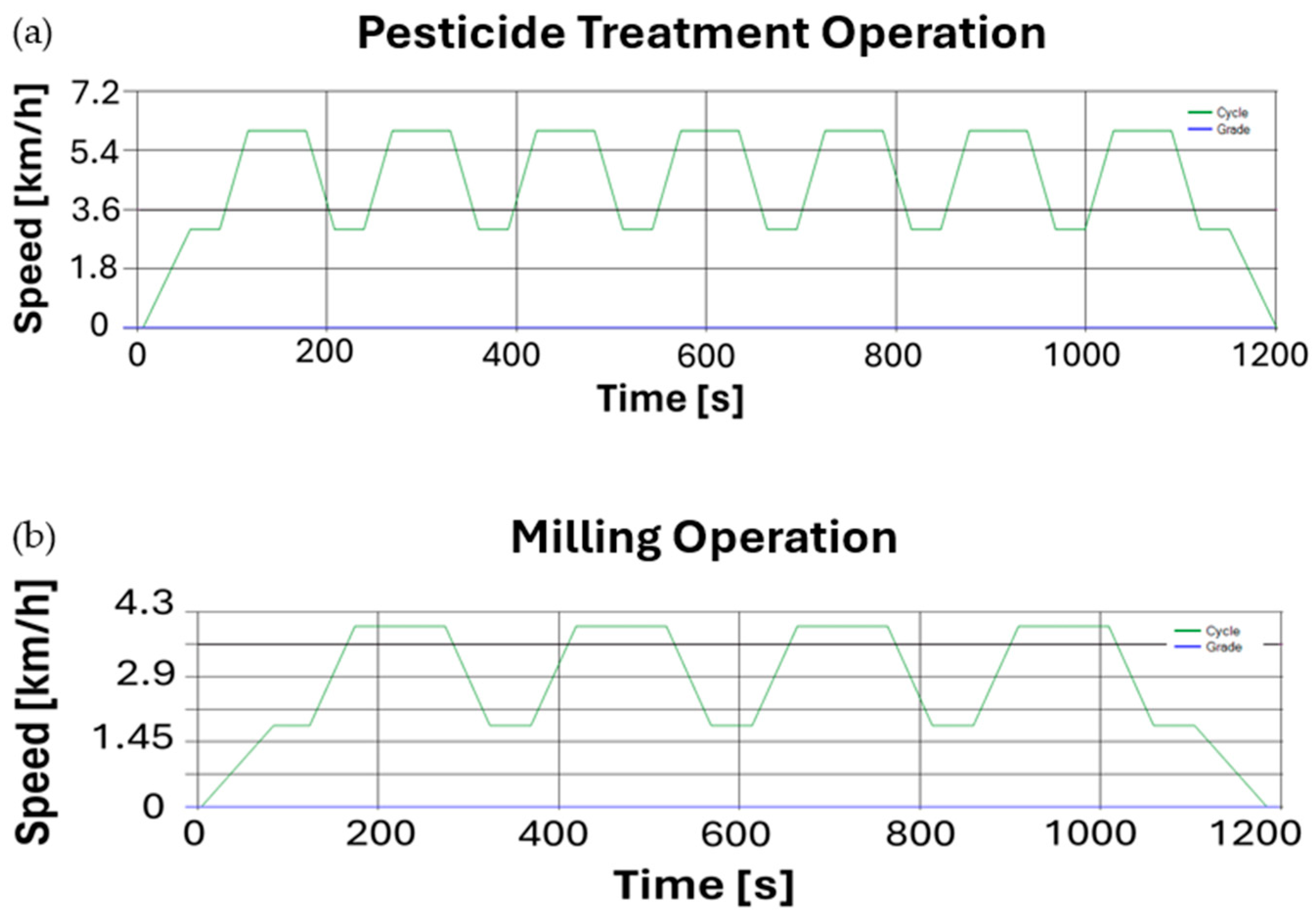
2.1.1. Pesticide Treatment

The execution of a pesticide treatment carried out in a “tendone” vineyard of a company located in the countryside of Castellaneta (TA) was considered. An air-assisted sprayer machine, AGRI IONICA model AGR/P [19] (AGRI IONICA SRL, Ginosa (TA), Italy), with a 1000 L tank, was towed in the field by the four-wheel drive Landini REX 4-120 GB tractor (Landini, Fabbrico, Italy, with a maximum power of 77 kW and a maximum torque of 420 Nm @ 1600 rpm (Figure 1)). The air-assisted sprayer machine was connected to the PTO of the Landini REX 4-120 GB tractor through an OC-SJ316-32 cardan joint produced by the company Octis S.r.l (Castiglione delle Stiviere, Italy), capable of transmitting a maximum torque of 600 Nm.

2.1.2. Milling Operation

A milling process was also considered, carried out with the DG45-400 Series milling machine (Forigo Roteritalia, Ostiglia, Italy), which was towed in the field by the four-wheel drive Fendt 942Vario tractor (AGCO GmbH, Marktoberdorf, Germany, with a maximum power of 261 kW and a maximum torque of 1970 Nm @ 1700 rpm) (Figure 2). The DG45-400 milling machine, connected to the tractor via a three-point hitch, was equipped with a hydraulic device for its opening and folding. The milling machine had 108 hoes, whose working depth was 0.28 m. The DG45-400 tiller was connected to the tractor’s PTO via a B-008 cardan joint produced by the company Benzi & Di Terlizzi Srl (Inzago, Italy), capable of transmitting a maximum torque of 2250 Nm.

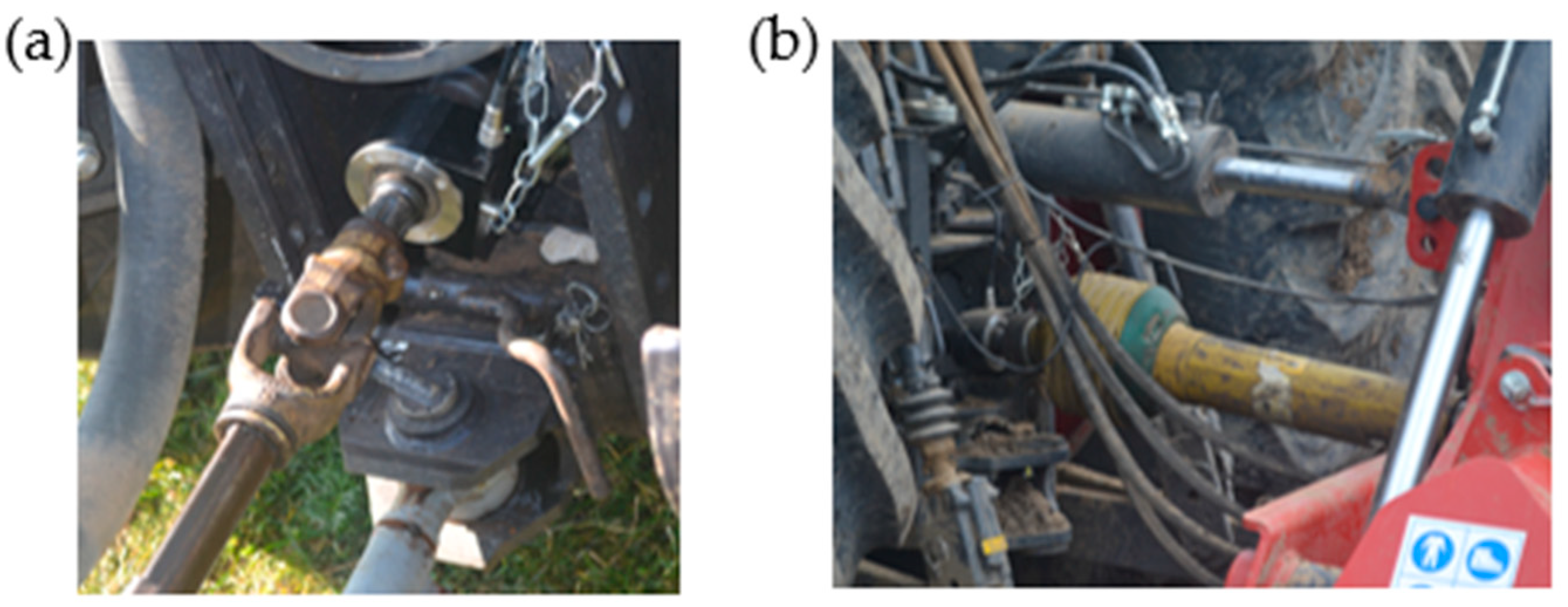
2.2. Shaft Torque and Power Monitoring System Transducer

During the execution of the two described field operations, the torque, the shaft speed, and the power at the PTO of the respective tractors were measured by a measuring system composed of the contactless rotary torque series 420 PTO Shaft Torque and Power Monitoring System transducer (Datum Electronics, Isle of Wight, UK) [20] and a control unit connected to a laptop through an RS232 cable. A custom software developed by the authors allowed the measured data to be displayed and logged. The technical features of the transducer were the following: accuracy of 0.5%; linearity +/− 0.1% FSD; repeatability +/− 0.05% FSD; sample rate from 1 to 100 samples s⁻¹; output baud rate of 9600 baud; and maximum torque of 2500 Nm. Figure 3 shows the rotary torque series 420 Shaft Torque and Power Monitoring System transducer inserted between the tractor PTO and the Hooke’s joint for the pesticide treatment (panel (a)) and for the milling operation (panel (b)), respectively.

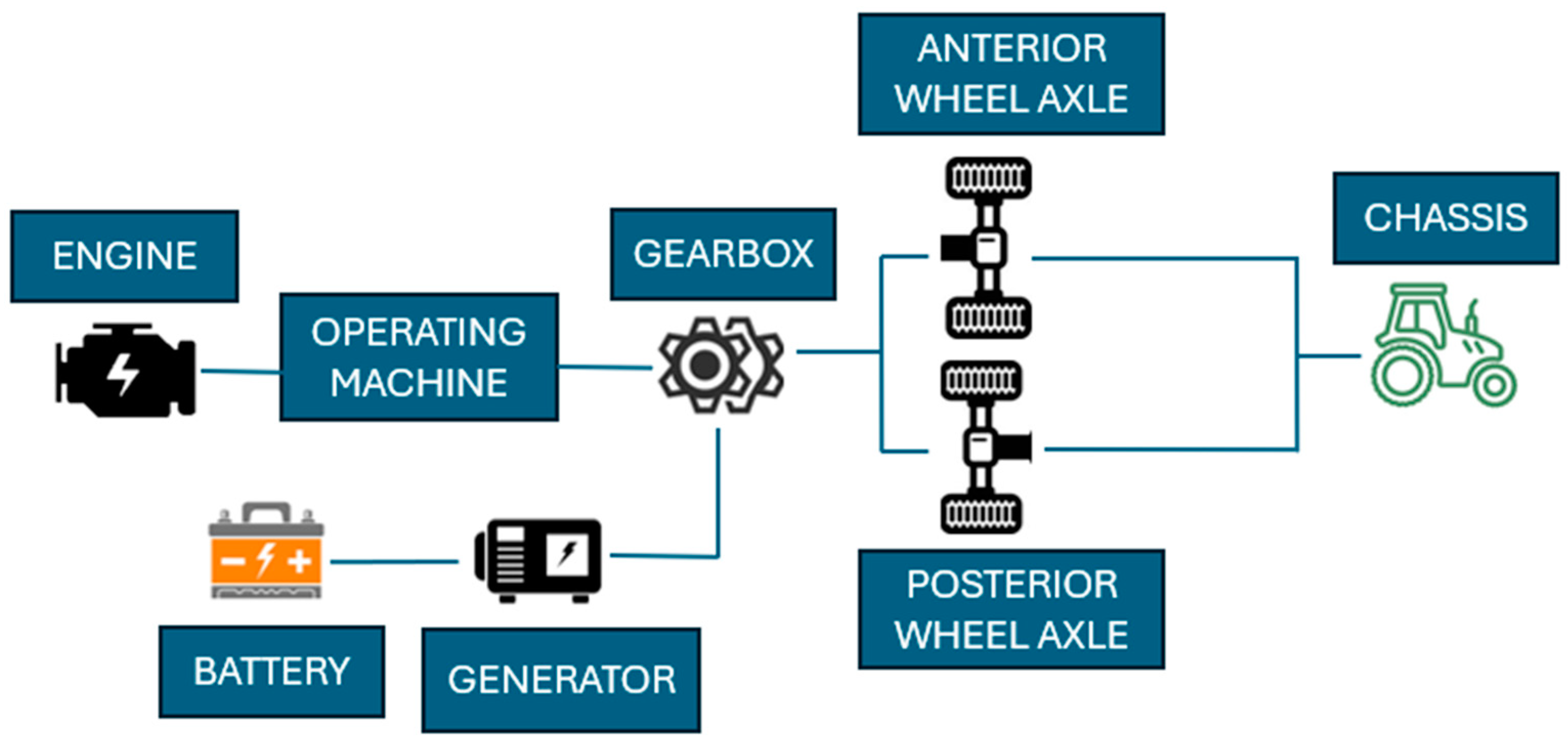
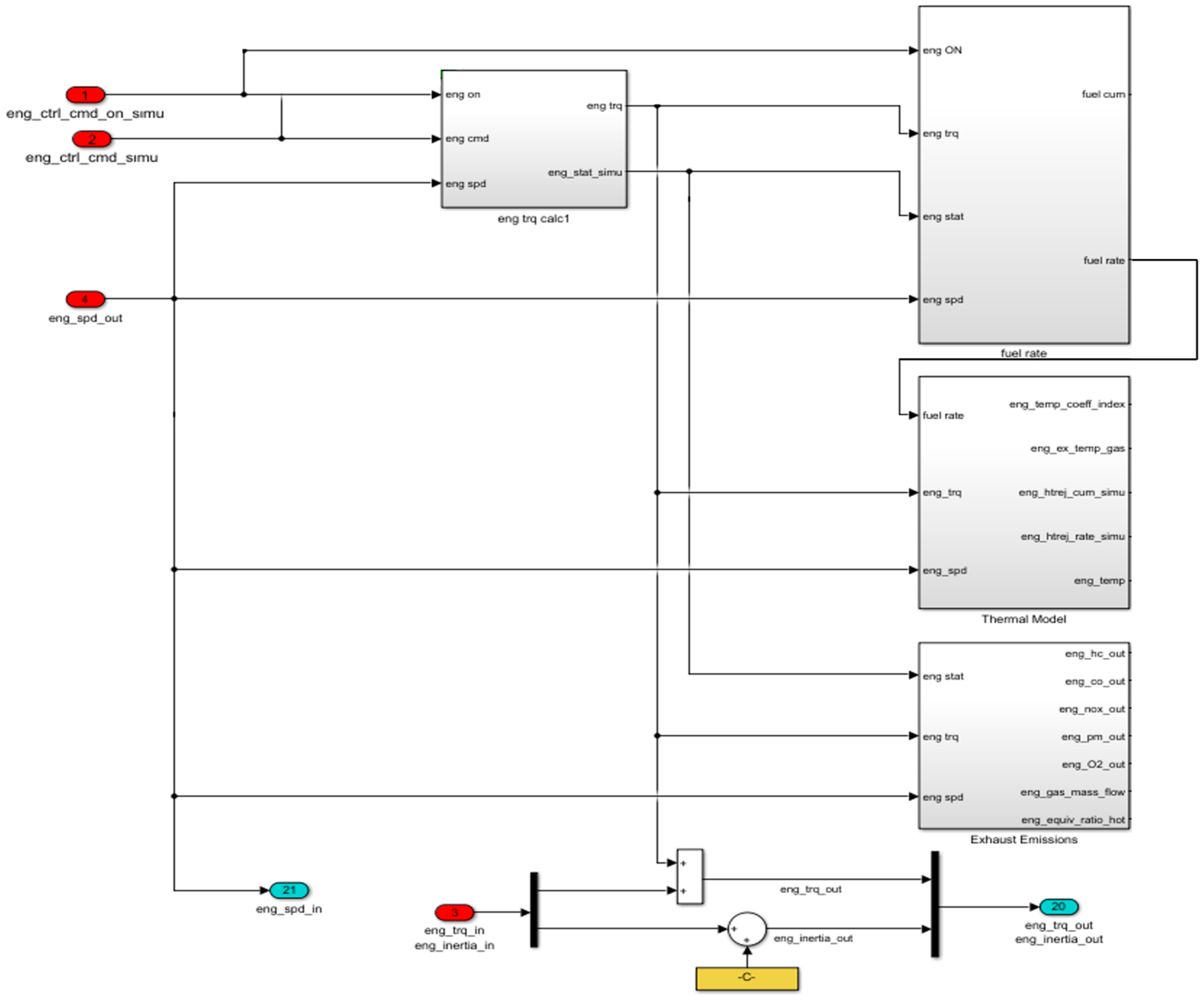
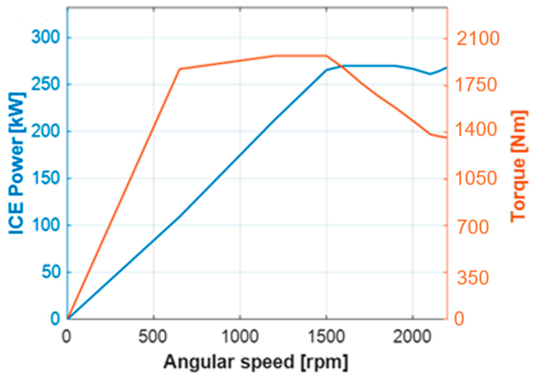
2.3. Modeling and Simulation Software

The modeling of the two agricultural tractors and the simulation of the execution of their respective field operations were performed using the software “Autonomie 2023” (https://www.anl.gov/taps/autonomie-vehicle-system-simulation-tool, accessed on 15 October 2024), developed by the Argonne National Laboratory Vehicle & Systems Mobility Group (VMS) [21]. The software is designed as an extensible model-based systems engineering (MBSE) platform used to create, customize, and deploy workflows, creating digital twins of vehicles. “Autonomie 2023” provides libraries for the modeling of the different vehicles’ components and includes control algorithms developed from vehicle dynamometer test data. The Vehicle Powertrain Controller (VPC) represents the high-level supervisory controller that manages vehicles’ control and decision-making. Its decisions are sent to the Vehicle Propulsion Architecture (VPA), which represents the powertrain systems and includes low-level controllers that execute the VPC demands. The software, originally designed for the simulation of on-road vehicles, has been adapted by the authors to simulate agricultural tractors. Modifications include the implementation of a new propulsion architecture, with changes in the configuration parameters of the powertrain and in vehicle dynamics. In this way, it has been possible to develop, in the “Autonomie 2023” software, the digital models of the Landini REX 4-120 GB and Fendt 942 Vario tractors. The schematic of the digital model of a tractor is presented in Figure 4. The software simulates vehicles’ performance during the execution of working cycles, providing output information about speed profile tracking, fuel consumption, and carbon footprints.

The digital model schematized in Figure 4 is composed of fundamental interconnected blocks. Both tractors have a four-wheel drive drivetrain and a diesel ICE with a five-speed automatic transmission. The gearbox efficiency has been set to 95% [22]. The operating machines, i.e., air-assisted sprayer and milling machine, have been modeled considering the power required at the PTO and their weight in the “Operating Machine” block directly connected to the engine. The software automatically builds each model’s subsystem in Simulink^® 2024a (MathWorks, Apple Hill Drive Natick, MA 01760, UNITED STATES) and interconnects them to create the entire vehicle’s model.

The Simulink^® model of the diesel ICE implemented in “Autonomie 2023” software is shown in Figure 5. It is divided into four fundamental blocks: Engine Torque Calculation, Engine Thermal Model, Engine Fuel Rate, and Exhaust Emissions. The red and cyan icons represent the inputs and the outputs of the Simulink^® model, respectively. The yellow rectangular is a mathematical constant.

The Engine Torque Calculation block calculates the torque produced by the ICE, interpolating between the maximum and minimum torque curves. This block has, as inputs, the $\mathrm{P}\mathrm{W}{\mathrm{M}}_{\mathrm{c}\mathrm{m}\mathrm{d}}$ engine command, given by the controller to the ICE, the $\mathrm{E}\mathrm{n}{\mathrm{g}}_{\mathrm{O}\mathrm{N}}$ command, which switches on the ICE, and the ${\mathsf{\omega }}_{\mathrm{e}\mathrm{n}\mathrm{g}}$, the angular speed of the engine. The block implements a finite-state machine with the following logic: if the torque commands ${\mathrm{T}}_{\mathrm{c}\mathrm{m}\mathrm{d}}$ and ${\mathsf{\omega }}_{\mathrm{e}\mathrm{n}\mathrm{g}}$ are greater than zero (${\mathrm{T}}_{\mathrm{c}\mathrm{m}\mathrm{d}}>0$, ${\mathsf{\omega }}_{\mathrm{e}\mathrm{n}\mathrm{g}}>0$) or if ${\mathrm{T}}_{\mathrm{c}\mathrm{m}\mathrm{d}}$ is equal to zero and ${\mathsf{\omega }}_{\mathrm{e}\mathrm{n}\mathrm{g}}$ is greater than zero (${\mathrm{T}}_{\mathrm{c}\mathrm{m}\mathrm{d}}=0$, ${\mathsf{\omega }}_{\mathrm{e}\mathrm{n}\mathrm{g}}>0$), the output torque is given by (1):

$${\mathrm{T}}_{\mathrm{o}\mathrm{u}\mathrm{t}}=(1-{\mathrm{T}}_{\mathrm{c}\mathrm{m}\mathrm{d}})·{\mathrm{T}}_{\mathrm{m}\mathrm{i}\mathrm{n}}+({\mathrm{T}}_{\mathrm{c}\mathrm{m}\mathrm{d}}·{\mathrm{T}}_{\mathrm{m}\mathrm{a}\mathrm{x}})$$

(1)

where ${\mathrm{T}}_{\mathrm{m}\mathrm{i}\mathrm{n}}$ is the minimum torque curve of the engine as a function of speed and T_max is the maximum torque curve of the engine as a function of speed. Otherwise, if T_cmd and ${\mathsf{\omega }}_{\mathrm{e}\mathrm{n}\mathrm{g}}$ are equal to zero (${\mathrm{T}}_{\mathrm{c}\mathrm{m}\mathrm{d}}=0$, ${\mathsf{\omega }}_{\mathrm{e}\mathrm{n}\mathrm{g}}=0$), the output torque is zero.

Figure 6 shows the implemented ICE power (blue line) and torque (orange line) curves of the Fendt 942 Vario tractor as a function of the angular engine speed.

The Engine Fuel Rate block is detailed in [23]. The Engine Thermal Model block takes the fuel rate ${\mathrm{F}}_{\mathrm{r}\mathrm{a}\mathrm{t}\mathrm{e}}$, ${\mathrm{T}}_{\mathrm{o}\mathrm{u}\mathrm{t}}$, and ${\mathsf{\omega }}_{\mathrm{e}\mathrm{n}\mathrm{g}}$ as inputs and calculates the instantaneous heat rejection $\mathrm{H}{\mathrm{t}}_{\mathrm{r}\mathrm{e}\mathrm{j}}$, given the GCV, through Formula (2):

$$\mathrm{H}{\mathrm{t}}_{\mathrm{r}\mathrm{e}\mathrm{j}}=({\mathrm{F}}_{\mathrm{r}\mathrm{a}\mathrm{t}\mathrm{e}}·\mathrm{G}\mathrm{C}\mathrm{V})-({\mathsf{\omega }}_{\mathrm{e}\mathrm{n}\mathrm{g}}·{\mathrm{T}}_{\mathrm{o}\mathrm{u}\mathrm{t}})$$

(2)

Finally, the Exhaust Emissions block calculates, through some implemented algorithms, the emissions, knowing ${\mathrm{T}}_{\mathrm{o}\mathrm{u}\mathrm{t}}$ and ${\mathsf{\omega }}_{\mathrm{e}\mathrm{n}\mathrm{g}}$.

The Simulink^® model of the chassis of the tractors is presented in Figure 7. The red and cyan icons represent the inputs and the outputs variables of the Simulink^® model, respectively. The yellow rectangular is a mathematical constant and the green rectangular trapezium is a temporary output variable.

The outputs of the model are the acceleration and speed of the tractors and the traveled distance. The net force acting on the chassis of the tractor is the difference between the force ${\mathrm{F}}_{\mathrm{t}\mathrm{r}\mathrm{a}\mathrm{c}\mathrm{t}}$, coming from the ICE, and the losses ${\mathrm{F}}_{\mathrm{l}\mathrm{o}\mathrm{s}\mathrm{s}}$ due to aerodynamic drag, grade, and rolling resistance.

$${\mathrm{F}}_{\mathrm{t}\mathrm{o}\mathrm{t}}={\mathrm{F}}_{\mathrm{t}\mathrm{r}\mathrm{a}\mathrm{c}\mathrm{t}}-{\mathrm{F}}_{\mathrm{l}\mathrm{o}\mathrm{s}\mathrm{s}}$$

(3)

The drag force has been considered, but it does not influence the results of the simulation because the tractor’s speed is very slow. Thus, its contribution is negligible. The grade is considered zero since the terrain on which the experimental tests were carried out was flat. The rolling resistance losses related to the wheels have been modeled by a fourth-degree polynomial that is a function of the tractor’s speed. The acceleration is obtained by dividing the net force ${\mathrm{F}}_{\mathrm{t}\mathrm{o}\mathrm{t}}$ by the mass of the system. Integrating the acceleration, it is possible to obtain the velocity, and by integrating a second time, we obtain the traveled distance.

Table 1. Main parameters of the simulated models.

Parameter	Landini REX 4-120 GB	Fendt 942 Vario
ICE Maximum Power @ 2200 rpm [kW]	77	261
Maximum Torque @ 1600 rpm [Nm]	420	1970
Mass of the tractor [kg]	2800	11,700
Anterior wheel radius [mm]	506	872
Posterior wheel radius [mm]	600	1084

reports the main technical specifications of the developed digital models of the Landini REX 4-120 GB and Fendt 942 Vario agricultural tractors, respectively.

Unlike the automotive sector, standardized working cycles for tractors have not yet been defined in the agricultural sector. Consequently, it is not possible to define a standard procedure for the evaluation of the energy inputs required during the execution of an agricultural operation [24]. The lack of standardized working cycles is strictly connected to the extreme heterogeneity of agricultural operations performed by agricultural tractors, which require a wide range of different and variable power absorptions, from a few tens of kW up to hundreds of kW [25]. Therefore, the field operations considered experimentally, i.e., pesticide treatment and soil milling, have been simulated in “Autonomie 2023” software, creating two different custom-defined working cycles that refer to the system tractor-operating machine. The two simulated working cycles have different working speeds and cornering speeds at the headland, as well as different accelerations and decelerations. Both working cycles last 1200 s. The defined working cycles are presented in Figure 8. They are composed of sequential phases. (i) The initial phases start at t₀ = 0 s, and considering that the system tractor-operating machine starts from a standstill (v = 0 m/s), it accelerates and reaches the starting point of the field operation; (ii) In the acceleration phase, the system tractor-operating machine accelerates to reach the desired working speed (6 km/h for pesticide treatment and 4 km/h for milling, respectively), maintaining it at a constant for a certain amount of time, in which the respective field operation is performed (60 s for pesticide treatment and 100 s for milling, respectively). (iii) In the deceleration phase, it decelerates to maneuver the headland turn with a lower speed (3 km/h for pesticide treatment and 2 km/h for milling, respectively). These sequential phases are repeated in the working cycle. At the end of the working cycle, the system decelerates up to the stop. The mean working speed of the system tractor-operating machine during pesticide treatment operation is 4.5 km/h, and it is 2.8 km/h for milling.

3. Results

3.1. Shaft Torque and Power Monitoring System Transducer Measurements

Several datasets have been acquired by the measuring system during the execution of the two described field operations. The acquired datasets were consistent; hence, it has been possible to consider only one of them. Figure 9 shows the control unit display reporting the instantaneous torque, angular speed, and power measured by the transducer at the tractor’s PTO.

Figure 10 reports the torque and the angular speed profile measured by the measuring system during the execution of pesticide treatment (panel (a)) and milling (panel (b)).

The minimum and maximum values, as well as the averages and standard deviations, of the torque, power, and angular speed measured at the PTO are reported in

Table 2. Basic statistics of the measured parameters.

Parameter	Min	Max	Average	Standard Deviation
AGRI IONICA model AGR/P
Angular Speed (rad/s)	56.1	56.5	56.4	0.1
Torque (Nm)	258.2	365.9	307.1	21.2
Power (kW)	14.5	20.7	17.3	1.2
Series DG45—400 milling machine
Angular Speed (rad/s)	99.8	102.2	101.1	0.5
Torque (Nm)	919.9	1808	1429.6	166.8
Power (kW)	91.8	184.8	144.5	16.6

.

Table 2 points out that the power required at the PTO by the air-assisted sprayer machine during its functioning is 17.3 kW on average. In contrast, the power required by the milling machine is 144.5 kW on average. The air-assisted sprayer machine operated at an average angular speed of the PTO of 56.4 rad/s (~539 rpm) and absorbed an average torque of 307.1 ± 21.2 Nm. The torque required by the air-assisted sprayer machine varies slightly from the average value because during the function of the machine, the fan and the pump, which put pressure on the hydraulic circuit, remained almost constant. On the other hand, Table 2 highlights that the milling operation required an average PTO angular speed of 101.1 rad/s (~966 rpm) and an average torque of 1429.6 ± 166.8 Nm. The high standard deviation value highlights that the torque required by this field operation strongly depends on the working conditions of the soil. The torque required by the milling machine is significantly higher than the spraying machine; the milling machine is much heavier and, when carrying out the operation at a working depth of 0.28 m, the machine requires greater power, which is absorbed by the tractor.

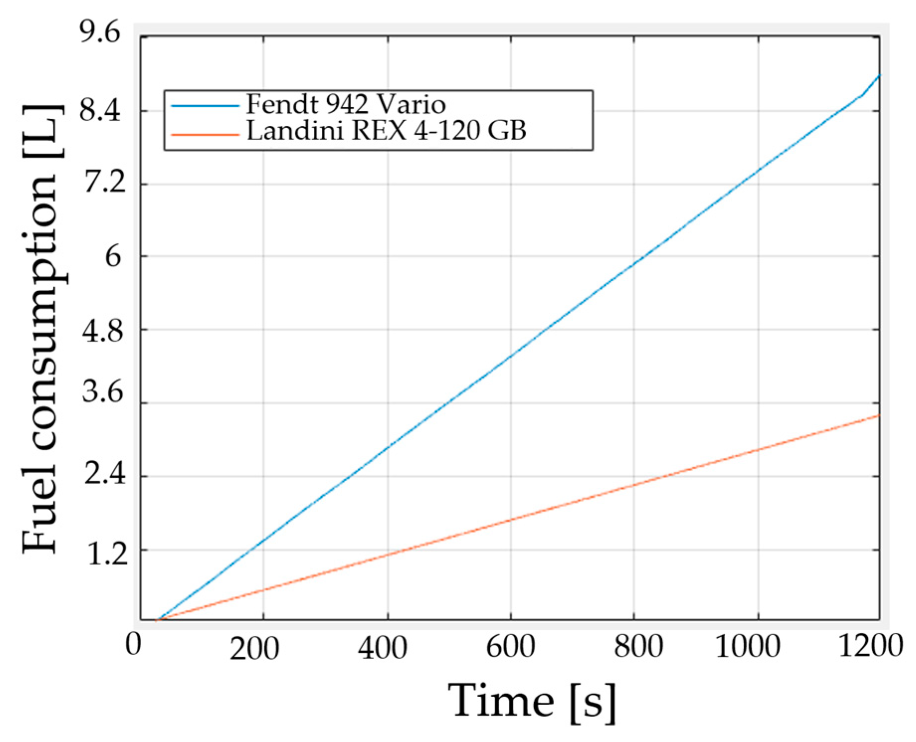
3.2. Simulation of Modeled Agricultural Tractors

In the developed digital models of the tractors, the experimentally measured power required by the operating machines during their operation and their mass have been included as parameters in the “Operating Machine” block directly connected to the engine. Thus, through this block, the losses related to the connected operating machines are considered. These parameters are summarized in

Table 3. Main parameters inserted in the “Operating Machine” block.

Parameter	AGRI IONICA Model AGR/P	Series DG45-400 Milling Machine
Mass [kg]	1350	3600
Mean Power required at PTO [kW]	17.3	144.5

.

The simulations were run at 100 Hz, using the fixed-step ode4 Runge–Kutta solver, with a time step of 0.01 s. Figure 8 reports, respectively, for the system Landini REX 4-120 GB–sprayer machine and for Fendt 942 Vario–milling machine, the actual working cycle carried out (orange line in Figure 11) and the imposed cycle (blue line in Figure 11). Figure 11 points out that the working cycles carried out by both systems are almost identical to those imposed. Thus, it is possible to state that the “Autonomie 2023” software, with some modifications to the configuration parameters of the powertrain and vehicle dynamics, is very reliable for creating digital models of agricultural tractors.

The fuel consumption of the Landini REX 4-120 GB and Fendt 936 Vario tractors, respectively, during the execution of the imposed working cycles is reported in Figure 12.

4. Discussion

The Simulink model utilized by the “Autonomie 2023” software to calculate the fuel consumption is described in [23]. Moreover, starting from the fuel consumption and evaluating the ICE working point during the working cycle, the software calculates CO₂ emissions [23]. The fuel consumption output from the software is given in L∙h⁻¹. To relate it to the working width of the employed operating machine, it was converted into L∙ha⁻¹, given the area covered by the tractor (expressed in ha) in one hour. The area is given by (4):

Area covered [ha∙h⁻¹] = Working speed [km∙h⁻¹] ∙ Working width [m] ∙ (K)

(4)

where K is the coefficient to convert the different units of measurement. Dividing the fuel consumption expressed in L∙h⁻¹ by the area covered calculated with (1), it is possible to obtain the fuel consumption in L∙ha⁻¹.

Table 4. Fuel required by the two tractors during the execution of the two defined working cycles and the respective CO₂ emissions.

Parameter	Landini REX 4-120 GB	Reference	Fendt 942 Vario	Reference	Fendt 942 Vario On-Board Instrumentation
Fuel Consumption [L∙ha−1]	7.8	7.0 [26]	23.2	24.0 [27]	25.2
CO2 emissions [kg∙ha−1]	26.5	*	68.4	*	*

* N/A.

reports the comparison of the fuel required by the Landini REX 4-120 GB and Fendt 942 Vario tractors during the execution of the working cycles, simulating the execution of pesticide treatment and milling. Moreover, the carbon footprint, in terms of CO₂ emissions, expressed in kg∙ha⁻¹, is reported.

Table 4 points out that the fuel consumption required by the two agricultural tractors is 7.8 L∙ha⁻¹ for the pesticide treatment and 23.2 L∙ha⁻¹ for milling, respectively. The data obtained from the simulation software are consistent with the data obtained by the tractors’ onboard instrumentation and reference values presented in the literature [26,27,28], which were obtained using expensive sensors. Moreover, Table 4 highlights that the estimated carbon footprint of the two agricultural tractors, represented by their CO₂ emissions, is equal to 26.5 kg_CO2 ha⁻¹ for the pesticide treatment and 68.4 kg_CO2 ∙ha⁻¹ for milling.

Assuming that the diesel is principally composed of C₁₂H₂₃ and assuming complete combustion, the chemical reaction ca be written as [29,30] (5):

$${\mathrm{C}}_{12}{\mathrm{H}}_{23}+18{\mathrm{O}}_2\to 12\mathrm{C}{\mathrm{O}}_2+11{\mathrm{H}}_2\mathrm{O}$$

(5)

From (5), it is possible to mathematically estimate the CO₂ generated by complete combustion because the fuel consumption has been calculated and the molecular weights of diesel (167 g/mol) and of CO₂ (44 g/mol) are known. The CO₂ emissions calculated in this way are equal to 23.5 kg_CO2∙ha⁻¹ for the pesticide treatment and 61.7 kg_CO2 ∙ha⁻¹ for the milling operation, respectively.

Considering the GCV of the diesel (38.5 MJ∙L⁻¹), it is possible to estimate the direct energy inputs supplied by the fuel and required by the two agricultural tractors through the relation (6):

Direct energy inputs [MJ∙ha⁻¹] = GCV [MJ∙L⁻¹] ∙ Fuel Consumption [L∙ha⁻¹]

(6)

The direct energy inputs required for the pesticide treatment and for the milling operation are equal to 300.3 MJ∙ha⁻¹ and 893.2 MJ∙ha⁻¹, respectively.

However, not all the energy supplied by the fuel is converted into useful mechanical work due to losses related to the engine, heat, friction, transmission, and the tractor–implement connection. The overall operational efficiency depends on the agricultural operation, and it is usually higher with light workloads. The tractor’s engine efficiency during spraying is higher compared to the engine efficiency during milling because the engine operates a relatively constant regime. On the contrary, during milling, the tractor’s engine is subjected to several changes in load and speed that worsen efficiency. The overall operational efficiency of the tractor–sprayer machine and the tractor–milling machine was set at 27% and 18%, respectively. These values are in line with the results presented in [31,32]. Considering the overall operational efficiency, the available mechanical work can be calculated as (7):

Available Mechanical Work [MJ∙ha⁻¹] = Direct energy inputs [MJ∙ha⁻¹] ∙ Overall Operational Efficiency

(7)

Using the relation (3), the amount of energy supplied by the fuel and effectively converted into available mechanical work is equal to 81.1 MJ∙ha⁻¹ and 160.8 MJ∙ha⁻¹ for the pesticide treatment and for the milling operation, respectively.

5. Conclusions

In this paper, the assessment of direct energy inputs required by two agricultural tractors, i.e., Landini REX 4-120 GB and Fendt 936 Vario, during the execution of pesticide treatment and milling, respectively, and the estimation of the carbon footprint have been carried out using “Autonomie 2023” simulation software. The digital models of the tractors were developed starting from real data obtained from field tests in which the power required by the two operating machines at the PTO was measured. Two custom working cycles, simulating the two agricultural operations, were defined and simulated. The results show that the direct energy inputs required for the engine are equal to 300.3 MJ∙ha⁻¹ and 893.2 MJ∙ha⁻¹ for the pesticide treatment and milling, respectively. The estimated carbon footprint is equal to 26.5 kg_CO2∙ha⁻¹ for pesticide treatment and 68.4 kg_CO2∙ha⁻¹ for milling. Considering the overall operational efficiency of the systems, the available mechanical work is 81.1 MJ∙ha⁻¹ for the pesticide treatment and 160.8 MJ∙ha⁻¹ for the milling operation. This study highlights the possibility of developing digital models of tractors in “Autonomie 2023” software and estimating direct energy inputs and the carbon footprint of tractors during the execution of field operations.

References

1. Singh, S.; Mittal, J.P. Energy in Production Agriculture; Mittal Publications: New Delhi, India, 1992. [Google Scholar]
2. Martinho, V.J.P.D. Direct and indirect energy consumption in farming: Impacts from fertilizer use. Energy 2021, 236, 121504. [Google Scholar] [CrossRef]
3. Lampridi, M.; Kateris, D.; Sørensen, C.G.; Bochtis, D. Energy Footprint of Mechanized Agricultural Operations. Energies 2020, 13, 769. [Google Scholar] [CrossRef]
4. Rokicki, T.; Perkowska, A.; Klepacki, B.; Bórawski, P.; Bełdycka-Bórawska, A.; Michalski, K. Changes in energy consumption in agriculture in the EU countries. Energies 2021, 14, 1570. [Google Scholar] [CrossRef]
5. Paris, B.; Vandorou, F.; Balafoutis, A.T.; Vaiopoulos, K.; Kyriakarakos, G.; Manolakos, D.; Papadakis, G. Energy use in open-field agriculture in the EU: A critical review recommending energy efficiency measures and renewable energy sources adoption. Renew. Sustain. Energy Rev. 2022, 158, 112098. [Google Scholar] [CrossRef]
6. Bowers, W. Agricultural field equipment. In Energy in Farm Production; Fluck, R.C., Ed.; Elsevier Science Publishers B.V.: Amsterdam, The Netherlands, 1992; pp. 117–129. [Google Scholar]
7. Felten, D.; Fröba, N.; Fries, J.; Emmerling, C. Energy balances and greenhouse gas-mitigation potentials of bioenergy cropping systems (Miscanthus, rapeseed, and maize) based on farming conditions in Western Germany. Renew. Energy 2013, 55, 160–174. [Google Scholar] [CrossRef]
8. Shamshirband, S.; Khoshnevisan, B.; Yousefi, M.; Bolandnazar, E.; Anuar, N.B.; Wahab, A.W.; Khan, S.U. A multiobjective evolutionary algorithm for energy management of agricultural systems—A case study in Iran. Renew. Sustain. Energy Rev. 2015, 44, 457–465. [Google Scholar] [CrossRef]
9. Aguilera, E.; Guzmán Casado, G.; Infante Amate, J. Embodied energy in agricultural inputs. In Documentos de Trabajo de la Sociedad de Estudios de Historia Agraria 1507; Sociedad Española de Historia Agraria: Madrid, Spain, 2015. [Google Scholar]
10. Grisso, R.D.; Perumpral, J.V.; Vaughan, D.H.; Roberson, G.T.; Pitman, R.M. Predicting tractor diesel fuel consumption. Agric. Eng. Int. CIGR J. 2010, 12, 67–74. [Google Scholar]
11. Lee, D.H.; Choi, C.H.; Chung, S.O.; Kim, Y.J.; Inoue, E.; Okayasu, T. Evaluation of tractor fuel efficiency using dynamometer and baler operation cycle. J. Fac. Agric. 2016, 61, 173–182. [Google Scholar] [CrossRef]
12. Alcock, R. Tractor-Implement Systems; Springer Science & Business Media: Berlin, Germany, 2012. [Google Scholar]
13. Balafoutis, A.; Beck, B.; Fountas, S.; Vangeyte, J.; Wal, T.V.d.; Soto, I.; Gómez-Barbero, M.; Barnes, A.; Eory, V. Precision Agriculture Technologies Positively Contributing to GHG Emissions Mitigation, Farm Productivity and Economics. Sustainability 2017, 9, 1339. [Google Scholar] [CrossRef]
14. Renius, K.T. Fundamentals of Tractor Design; Springer: Cham, Switzerland, 2020. [Google Scholar]
15. Mantoam, E.J.; Romanelli, T.L.; Gimenez, L.M. Energy demand and greenhouse gases emissions in the life cycle of tractors. Biosyst. Eng. 2016, 151, 158–170. [Google Scholar] [CrossRef]
16. Zamagni, A.; Masoni, P.; Buttol, P.; Raggi, A.; Buonamici, R. Finding life cycle assessment research direction with the aid of meta-analysis. J. Ind. Ecol. 2012, 16, S39–S52. [Google Scholar] [CrossRef]
17. Lovarelli, D.; Fiala, M.; Larsson, G. Fuel consumption and exhaust emissions during on-field tractor activity: A possible improving strategy for the environmental load of agricultural mechanisation. Comput. Electron. Agric. 2018, 151, 238–248. [Google Scholar] [CrossRef]
18. Paciolla, F.; Patimisco, P.; Farella, A.; Quartarella, T.; Pascuzzi, S. Performance evaluation of hybrid-electric architectures for agricultural tractors. In Proceedings of the International Symposium on Farm Machinery and Processes Management in Sustainable Agriculture, Cham, Switzerland, 12–14 June 2024; Springer Nature: Cham, Switzerland, 2024; pp. 346–356. [Google Scholar]
19. Pascuzzi, S. The effects of the forward speed and air volume of an air-assisted sprayer on spray deposition in tendone trained vineyards. J. Agric. Eng. 2013, 44, e18. [Google Scholar] [CrossRef]
20. Crolla, D.A. Torsional Vibration Analysis of tractor and machine PTO drivelines. J. Agric. Eng. Res. 1978, 23, 259–272. [Google Scholar] [CrossRef]
21. Karbowski, D.; Pagerit, S. Autonomie 2023, a plug-and-play software architecture. In Proceedings of the Vehicle Power and Propulsion Conference, Lille, France, 1–3 September 2010; pp. 1–3. [Google Scholar]
22. Kim, Y.-S.; Kim, W.-S.; Siddique, M.A.A.; Baek, S.-Y.; Baek, S.-M.; Cheon, S.-H.; Lee, S.-D.; Lee, K.-H.; Hong, D.-H.; Park, S.-U.; et al. Power Transmission Efficiency Analysis of 42 kW Power Agricultural Tractor According to Tillage Depth during Moldboard Plowing. Agronomy 2020, 10, 1263. [Google Scholar] [CrossRef]
23. Pascuzzi, S.; Łyp-Wrońska, K.; Gdowska, K.; Paciolla, F. Sustainability Evaluation of Hybrid Agriculture-Tractor Powertrains. Sustainability 2024, 16, 1184. [Google Scholar] [CrossRef]
24. Koniuszy, A.; KostencKi, P.; Berger, A.; Golimowski, W. Power performance of farm tractor in field operations. Eksploat. Niezawodn. 2017, 19, 43–47. [Google Scholar] [CrossRef]
25. Adewoyin, A.O.; Ajav, E.A. Fuel consumption of some tractor models for ploughing operations in the sandy-loam soil of Nigeria at various speeds and ploughing depths. Agric. Eng. Int. CIGR J. 2013, 15, 67–74. [Google Scholar]
26. Cech, R.; Leisch, F.; Zaller, J.G. Pesticide Use and Associated Greenhouse Gas Emissions in Sugar Beet, Apples, and Viticulture in Austria from 2000 to 2019. Agriculture 2022, 12, 879. [Google Scholar] [CrossRef]
27. Fathollahzadeh, H.; Mobli, H.; Tabatabaie, S. Effect of ploughing depth on average and instantaneous tractor fuel consumption with three-share disc plough. Int. Agrophys. 2009, 23, 399–402. [Google Scholar]
28. Moitzi, G.; Haas, M.; Wagentristl, H.; Boxberger, J.; Gronauer, A. Energy consumption in cultivating and ploughing with traction improvement system and consideration of the rear furrow wheel-load in ploughing. Soil Tillage Res. 2013, 134, 56–60. [Google Scholar] [CrossRef]
29. Gupta, H.N. Fundamentals of Internal Combustion Engines; PHI Learning Pvt. Ltd.: New Delhi, India, 2012. [Google Scholar]
30. Mollenhauer, K.; Tschöke, H. (Eds.) Handbook of Diesel Engines; Springer: Berlin, Germany, 2010; Volume 1. [Google Scholar]
31. Ortiz-Cañavate, J.; Gil-Sierra, J.; Casanova-Kindelán, J.; Gil-Quirós, V. Classification of agricultural tractors according to the energy efficiencies of the engine and the transmission based on OECD tests. Appl. Eng. Agric. 2009, 25, 475–480. [Google Scholar] [CrossRef]
32. Al-Sager, S.M.; Almady, S.S.; Marey, S.A.; Al-Hamed, S.A.; Aboukarima, A.M. Prediction of specific fuel consumption of a tractor during the tillage process using an artificial neural network method. Agronomy 2024, 14, 492. [Google Scholar] [CrossRef]
Figure 1. The AGRI IONICA model AGR/P air-assisted sprayer machine towed by the Landini REX 4-120 GB tractor during pesticide treatment. Source: Author’s personal archive.
Agriengineering 07 00007 g001
Figure 2. Series DG45-400 milling machine towed by the Fendt 942 Vario tractor during the milling operation. Source: Author’s personal archive.
Agriengineering 07 00007 g002
Figure 3. Rotary torque series 420 Shaft Torque and Power Monitoring System transducer linked between the PTO and the Hooke’s joint connected to (a) the Landini REX 4-120 GB for pesticide treatment and (b) the Fendt 942 Vario for milling operation. Source: Author’s personal archive.
Agriengineering 07 00007 g003
Figure 4. Schematic of the digital model of the tractor. Source: Author’s personal archive.
Agriengineering 07 00007 g004
Figure 5. Simulink® model of the Engine block. Source: Screenshot from the “Autonomie 2023” software.
Agriengineering 07 00007 g005
Figure 6. Power (blue line) and torque (orange line) profiles of the Fendt 942 Vario tractor. Source: Modified in MATLAB 2023a (MathWorks).
Agriengineering 07 00007 g006
Figure 7. Simulink® model of the Chassis block. Source: Screenshot from the “Autonomie 2023” software.
Agriengineering 07 00007 g007
Figure 8. Custom-defined working cycle which simulates (a) pesticide treatment operation and (b) milling operation. Source: Screenshot from “Autonomie 2023” software modified by the authors.
Agriengineering 07 00007 g008
Figure 9. Control unit display reporting the instantaneous torque, angular speed, and power measured by the transducer at the tractor’s PTO. Source: Author’s personal archives.
Agriengineering 07 00007 g009
Figure 10. Torque and the PTO angular speed profile as a function of time, measured by the 420 PTO Shaft Torque and Power Monitoring System transducer, during the execution of (a) the spraying operation and (b) the burying operation. Source: Modified by the authors in MATLAB 2023a (MathWorks).
Agriengineering 07 00007 g010
Figure 11. Speed profile followed by (a) the system Landini REX 4-120 GB–sprayer machine and (b) the Fendt 942 Vario–milling machine during the defined working cycles. Source: Modified by the authors in MATLAB 2023a (MathWorks).
Agriengineering 07 00007 g011
Figure 12. Fuel consumption of Landini REX 4-120 GB (orange line) and Fendt 942 Vario (blue line) tractors during the defined working cycles. Source: Modified by the authors in MATLAB 2023a (MathWorks).
Agriengineering 07 00007 g012