Optimizing Cotton Cultivation Through Variable Rate Seeding: An Enabling Methodology

Abstract

This study develops a practical, on-farm methodology for optimizing cotton cultivation through Variable Rate Seeding (VRS), utilizing existing farm data and remote sensing, while minimizing operational interference. The methodology involved an experimental design across five rainfed cotton fields on a Brazilian commercial farm, testing four seeding rates (90%, 100%, 110%, 120%) within grid cells using a 4 × 4 Latin square design. Management zones (MZs) were defined using existing soil clay content and elevation data, augmented by twelve vegetation indices from Sentinel-2 satellite imagery and K-Means clustering. Statistical analysis evaluated plant population density’s effect on cotton yield and its association with MZs. For the 2023/2024 season, results showed no positive yield response to increasing plant density above field averages, with negative responses in many plots (e.g., 84% in Field A), suggesting potential gains from reducing rates. The association between population density effect classes and MZs was highly significant with moderate to relatively strong Cramer’s V values (up to 0.47), indicating MZs effectively distinguished response areas. Lower clay content consistently correlated with yield losses at higher densities. This work empowers farm managers to conduct their own site-specific experimentation for optimal seed populations, enhancing precision agriculture and resource efficiency.

1. Introduction

Crops such as corn and cotton exhibit considerable yield variability due to differences in soil fertility, moisture capacity, and other local conditions, making variable rate seeding (VRS) a promising approach to boost both productivity and sustainability. VRS is an advanced precision agriculture strategy designed to improve crop performance by adapting seeding rates to the variability in soil characteristics, seed cultivar suitability, topography, and environmental factors in a field. This contrasts with the conventional uniform seeding method, which uses a constant seed rate throughout the field, often resulting in inefficient resource use and spatial yield variability, especially in fields exhibiting large spatial or anthropic spatial variability. Overall, studies agree that adapting seeding rates to field variability enhances resource efficiency and yield consistency. The fundamental concept of VRS is to align the seed rates with the specific needs of different management zones (MZ) within a field. For example, areas with fertile soil may benefit from denser plant populations to maximize yields, while less fertile zones may require lower seed rates to prevent excessive competition for scarce resources. By customizing seeding rates, farmers can optimize the use of inputs such as seeds, fertilizers, and water, which could lead to better economic returns and lower environmental impacts. This site-specific adjustment is widely linked to higher input efficiency and sustainability.

Anselmi et al. [1] demonstrated that MZ specific seeding is a cost-effective strategy that boosts yields while lowering expenses with seeds. For large-scale implementation, the feasibility of VRS is further enhanced by Speranza et al. [2]. They showed that vegetation indices (VIs) alone can be sufficient to delineate these MZs, simplifying the process, and making precision seeding more accessible for broader adoption. These findings point toward more practical and scalable VRS applications through remote sensing.

Šarauskis et al. [3] found that using VRS equipment on 400 ha of arable land leads to a one-year payback period, with an average benefit of around 100 EUR per hectare. Their research also concluded that VRS is effective for farms averaging at least 150 ha. For cotton, where plant density plays a critical role in boll formation and overall yield, fine-tuning seeding rates based on soil properties can reduce costs and improve fiber quality [4]. Thus, economic assessments generally support the profitability of VRS in large-scale operations.

Research on the effect of plant density on cotton lint yield presents contrasting findings, often influenced by water availability (

Table 1. Summary of cotton yields and plant densities from cited research.

Source	Plant Density (plants ha−1)	Yield Type	Yield (kg ha−1)	Conditions/Notes
Kimura et al. [5]	54,078	Lint	1199	Deficit-irrigated; Optimized for net return.
	67,346		796	Dryland; Optimized for net return.
Khan et al. [4]	87,000	Lint	1682	Reported as highest yield density.
		Seed Cotton	4546
Khan et al. [6]	87,000	Lint	1763	Reported as highest yield density.
		Seed Cotton	4662

). For instance, Kimura et al. [5] investigated yields in a water-scarce environment, finding no statistical differences across various population densities. However, their study suggested that lower final plant densities optimized net return when compared to higher densities. This implies that producers in water-scarce regions might achieve acceptable economic benefits by reducing seeding rates, even with statistically similar yields. In contrast, studies by Khan et al. [4,6] consistently reported that a specific higher plant density resulted in the highest seed cotton and lint yields (see Table 1 for specific values). Both studies noted that increasing plant density beyond this optimum led to a decrease in yield, attributing the enhanced yield at the optimal density to greater biomass accumulation in reproductive organs. Overall, water availability emerges as a key factor explaining the contrasting yield-density relationships.

Boyer et al. [7] also observed a curvilinear relationship between the seeding rate and the lint yield, where the yield decreased beyond an optimum. Their research identified a yield-maximizing seeding rate, which is listed in Table 1. However, they distinguished this from profit-maximizing objectives, which often lead to different recommendations [7]. These authors concluded that profit-maximizing rates depend on both cotton lint and seed prices; as seed prices increase, the optimal seeding rate for profit decreases. In contrast, an increase in cotton prices leads to an increase in the optimal seeding rate. For example, with a seed price of $5 per 1000 seeds, optimal profit-maximizing seeding rates (shown in Table 1) were identified when the assumed prices for cotton varied from $1.1 to $1.7 kg⁻¹. These profit-maximizing rates were consistently lower than the rate identified for maximizing yield. Hence, most economic analyses show that profit-maximizing seeding rates are lower than yield-maximizing ones.

Further supporting this distinction, Kimura et al. [5] observed that under dryland conditions, lower population densities significantly increased net returns due to reduced seed costs, even when lint yields were statistically similar across different densities. In contrast, irrigated trials showed consistent net returns across all tested population densities. While Khan et al. [6] reported that the optimal plant density for lint yield (see Table 1) also produced the highest net returns, they acknowledged that seed and labor costs substantially impacted profitability. They noted that lower plant densities might sometimes necessitate increased labor for specific field management practices, such as vegetative branch removal. Together, these findings indicate that profitability depends on both input costs and production environment.

The intricate relationship between plant density and cotton yield is modulated by a confluence of environmental and management factors. These include, but are not limited to, geographical location, precipitation levels, heat unit accumulation, soil type, planting dates, tillage practices, the presence of previous crops or cover crops, and fertility and weed control programs [4,5]. Row spacing also plays a critical role. In environments with limited water availability, lower plant densities are frequently identified as optimal [5]. Additionally, delayed planting dates typically reduces yield potential, and in such scenarios, reducing the seeding rate can become a profit-maximizing decision. Collectively, these studies emphasize that seeding optimization requires integrating agronomic, climatic, and management variables.

While the aforementioned research clearly demonstrates the significant potential of VRS to enhance yields, reduce costs, and improve sustainability in various crops (including corn and cotton), widespread adoption of this promising technology remains notably limited. Despite the demonstrated economic benefits, such as a rapid payback period and substantial returns per hectare, farmers continue to face considerable hurdles, including the initial investment in specialized equipment, the complexity of sophisticated data collection and analysis, and the need for specialized expertise to develop precise, site-specific seeding prescriptions. Most authors agree that adoption barriers are primarily technical and financial, not agronomic. Ongoing advancements in precision agriculture, particularly the improvement of spatial data precision and the increase in technology accessibility, are crucial to overcoming these barriers and providing the robust economic evidence necessary to accelerate the broader integration of VRS into diverse agricultural systems.

Although the referenced literature presents promising results, a critical limitation is evident: most of the studies were carried out under strictly controlled conditions on small experimental plots within research institutions. Only Anselmi et al. [1] incorporated on-farm experimentation, which was exclusively focused on maize seeding rates, in a commercial farm. Generalizing recommendations for optimal seed populations from such constrained environments remains challenging due to the vast diversity in soil properties, climatic conditions, and existing cultural practices encountered across commercial agricultural landscapes. This limitation underscores the need for more on-farm studies to validate VRS performance at operational scales. Furthermore, it is crucial to acknowledge the scale of real-world operations; the fields studied in our work range from 78 to 332 ha, commonly managed with fleets of up to five planters and as many as fifteen combines during sowing and harvesting, respectively.

Recognizing these fundamental differences, the present research focused on on-farm investigation within a commercial operation. The primary objective of this study was to establish a practical, data-driven methodology that enabled farm managers to determine the seed population that maximized return on investment under their specific field conditions. This approach was developed under the hypothesis that the essential spatial and operational data required for this analysis were already available on most farms. In doing so, the work aimed to empower farm managers to conduct their own site-specific experimentation with minimal disruption to routine operations.

2. Materials and Methods

2.1. Experimental Design

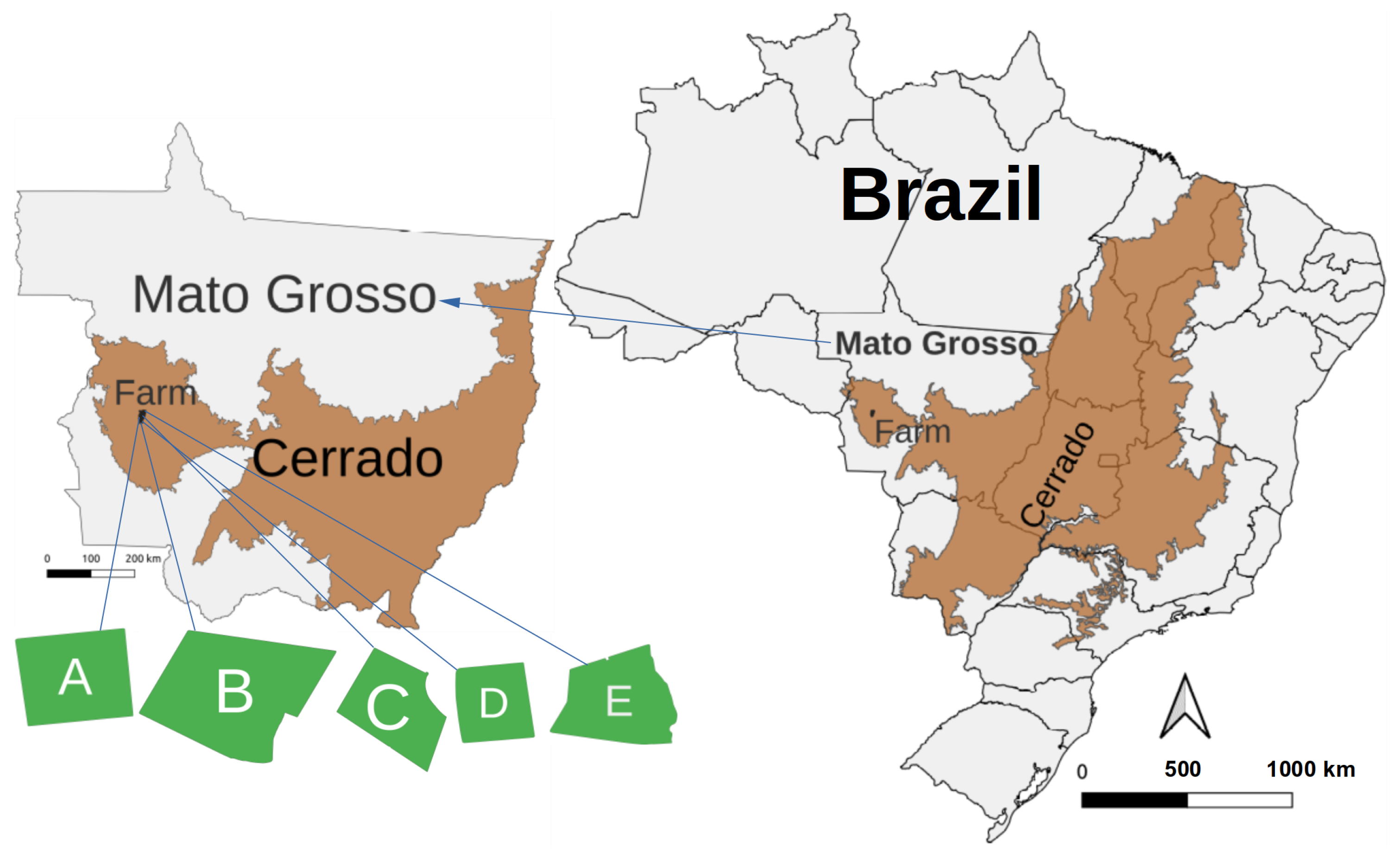
The cotton experiment was conducted in five rainfed fields on the commercial farm Tucunaré, which is part of the Amaggi Group and located in Sapezal, Mato Grosso, Brazil (12°59′22″ S, 58°45′51″ W) (Figure 1). This site is within the Cerrado biome, the largest tropical savanna in the world, spanning 198.455 Mha and covering 23.3% of the Brazilian territory [8]. These relatively flat fields typically operate under a no-tillage double-cropping system, with soybeans cultivated in the spring-summer period and cotton in the summer-fall-winter period.

Table 2. Experimental field characteristics: Area, altitude, and soil clay content (mean ± standard deviation).

Field	Sowing-Harvest Dates	Area (ha)	Altitude Range (m)	Clay (%)
				Range	Mean	SD
A	19 Feb 2023–15 Aug 2023	262	512–594	12–69	40.8	18
	06 Jan 2024–01 Sep 2024	196	571–594	21–69	48.7	13
B	22 Jan 2024–06 Sep 2024	332	547–580	23–66	50.3	12
C	19 Jan 2024–20 Aug 2024	186	534–580	15–67	39.5	15
D	26 Dec 2023–10 Jul 2024	78	546–564	12–20	15.6	2
E	13 Jan 2024–11 Aug 2024	224	549–573	26–62	42.4	9

details the characteristics of each experimental field and its corresponding cotton season. The predominant soil type in the five fields is dystropic red latosol (Oxisol). Notably, while fields B through E provided data only for the 2023/24 harvest season, Field A uniquely offered data from two consecutive cotton seasons: 2022/23 and 2023/24. For the second season, the farm manager decided to reduce the planted area of Field A by excluding a sandy region that had previously produced very low yields.

The fertilization management was applied as follows:

• N: A total of 170 kg ha⁻¹ was applied in four top-dressing splits: one-fifth at 15, 30, and 70 days after sowing (DAS), and the remaining two-fifths at 45 DAS.
• P: 40 kg ha⁻¹ was applied as a single dose at sowing.
• K: A total of 160 kg ha⁻¹ was applied in three splits: one-fourth at sowing, one-fourth at 30 DAS, and half at 70 DAS.
• S: A total of 70 kg ha⁻¹ was applied in two equal splits at 30 and 70 DAS.
• B: A total of 3 kg ha⁻¹ was applied, with one-third at sowing and the remaining two-thirds as a top-dressing at 30 DAS.

Elevation data for all fields were precisely collected using the Real Time Kinematic GPS (RTK-GPS) monitor of a combine harvester, while a clay content map was generated through kriging interpolation from soil samples taken at a density of one sample per 5 ha.

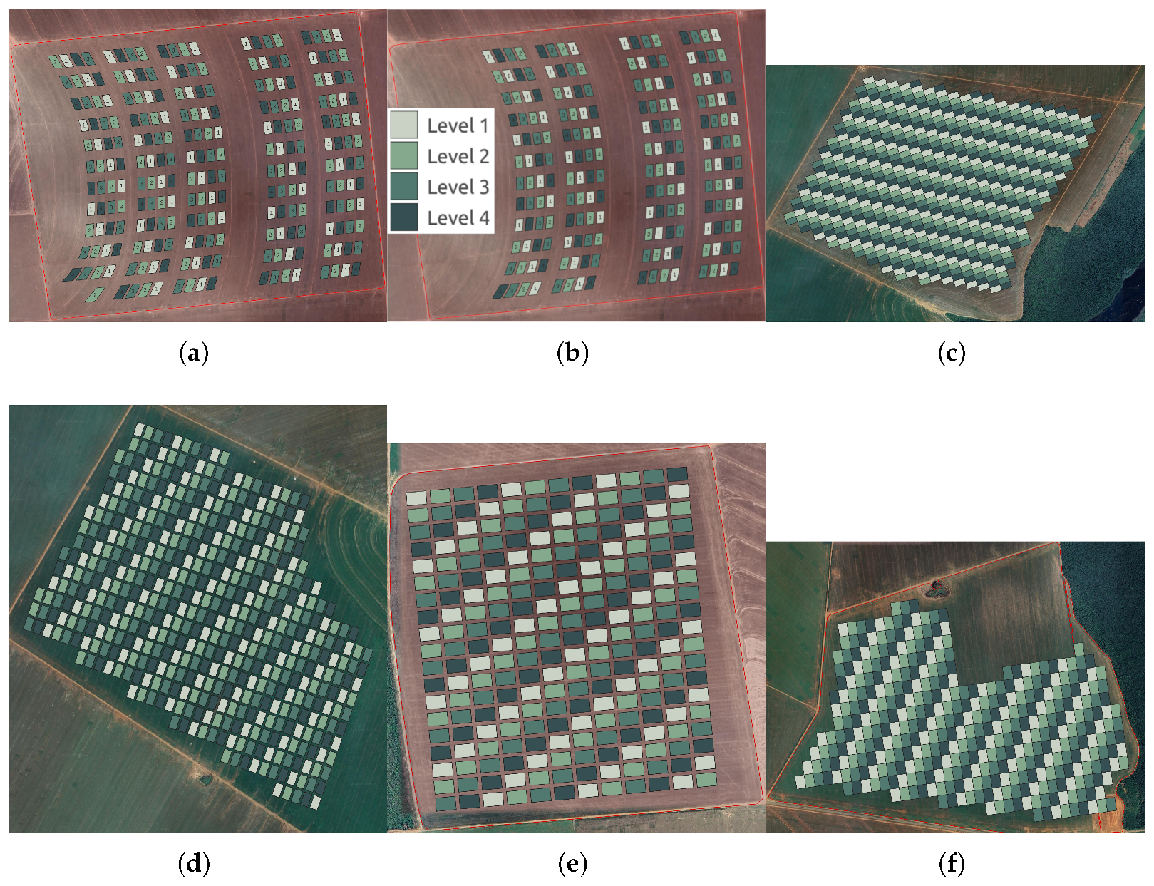
The trial methodology evaluated four seeding rates: 90%, 100% (100% represents the recommended dose. The application range of 90% to 120% was determined by the farm manager based on operational discretion and risk tolerance.), 110%, and 120% of the recommended seed companies’ rates (

Table 3. Cotton cultivars, recommended population (Rcmd Pop) and cell size (W: width, L: length), W is defined by two passes of planter.

Field	Cotton Cultivar	Cycle (days)	Rcmd Pop (plants m−1)	Planter Rows *	Cell Size (W × L) (m)	N Cells
A (22/23)	TMG22 GLTP	140 to 220	7 to 8	22	40.2 × 70	237
A (23/24)				22	40.2 × 70	192
B				24	43.9 × 80	688
C				19	34.7 × 50	479
D	IMA5801 B2RF	140 to 180	8	19	34.7 × 60	228
E	TMG31 B3RF	140 to 180	8 to 9	30	54.9 × 80	324

* Spacing for all fields is 0.9144 m (3 feet). To convert seeds m⁻¹ to seeds ha⁻¹, multiply by 10,936.1330 m ha⁻¹.

). These populations were applied within defined grid cells, also known as virtual plots (Figure 2), established within the fields. For all fields, rows were spaced at 3 feet (0.9144 m), with each grid cell’s width determined by two passes of the planter. Table 3 also details the dimensions and number of cells according to the planter, determined by farm logistics, and its respective number of rows.

The farm manager made the yield maps available, which were normalized by the weight of the cotton bales harvested by each John Deere CP690. This normalization is necessary to minimize differences in calibration between multiple machines. The yield monitor on the harvester measures the mass flow rate of the cotton being conveyed to the harvester’s basket. The John Deere CP690 specifically uses a microwave sensor that measures the mass flow rate and moisture content as cotton travels through the air ducts. This data, combined with an RTK-GPS signal for location and other machine data, such as speed, is used to calculate and create a detailed yield map for the field. While microwave sensors are susceptible to environmental factors like humidity, proper calibration and normalization procedures help ensure the accuracy of the final yield map. Due to the humidity influence on cotton mass, it is important to harvest the entire field in the same period of the day.

The four populations were distributed in grid cells using a 4 × 4 Latin square design as shown in (Figure 2).

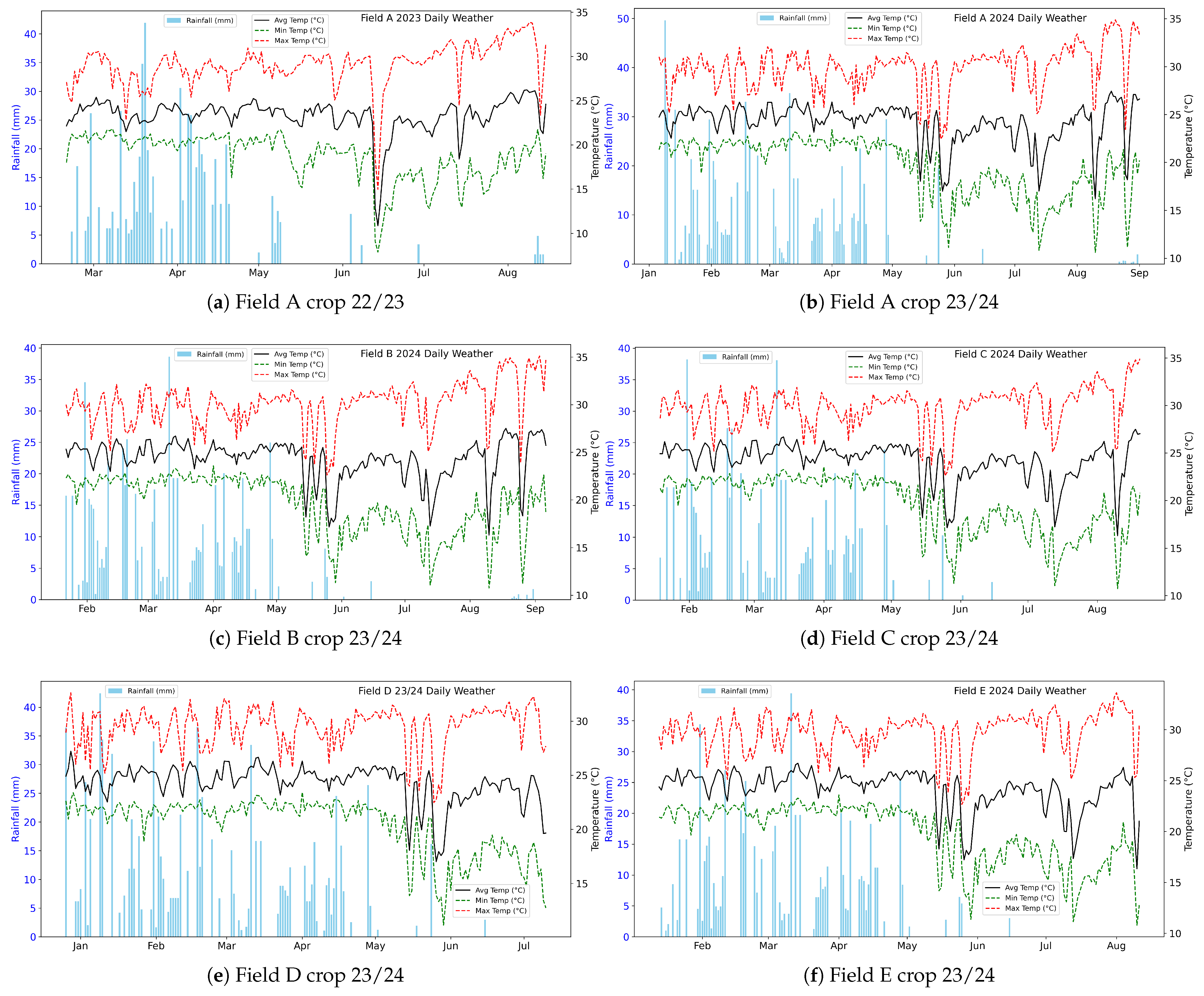
The climate of the region is characterized as tropical monsoon (Am) according to the Köppen climate classification [9], and the shapefiles of the climate zones of Brazil were obtained in [10]. The rainfall distribution and temperatures during each crop season are presented in

Table 4. Accumulated precipitation (mm) and averaged temperatures (ºC) in 30 DAS periods.

Field		A 22/23	A 23/24	B	C	D	E
Sowing Date		19 Feb 23	06 Jan 24	22 Jan 24	19 Jan 24	26 Dec 23	13 Jan 24
Harvest Date		15 Aug 23	01 Sep 24	06 Sep 24	20 Aug 24	10 Jul 24	11 Aug 24
1–30	Acc. Precipitation	284	271	246	217	288	196
	Avg. Minimum Temperature	20.7	21.6	21.9	21.9	21.7	21.8
	Avg. Temperature	23.6	24.8	25.0	25.2	24.7	25.0
	Avg. Maximum Temperature	27.9	29.4	29.4	29.7	29.1	29.5
31–60	Acc. Precipitation	281	182	163	197	244	204
	Avg. Minimum Temperature	20.5	21.7	22.0	22.0	21.7	22.0
	Avg. Temperature	23.8	24.9	25.3	25.1	24.8	25.1
	Avg. Maximum Temperature	28.4	29.4	30.0	29.7	29.2	29.7
61–90	Acc. Precipitation	34	163	183	193	137	157
	Avg. Minimum Temperature	19.4	22.2	22.2	22.3	22.0	22.3
	Avg. Temperature	23.7	25.1	24.7	24.8	25.2	25.1
	Avg. Maximum Temperature	29.0	29.6	28.9	28.9	29.9	29.3
91–120	Acc. Precipitation	12	140	40	42	156	91
	Avg. Minimum Temperature	17.1	21.9	20.2	20.7	22.1	21.6
	Avg. Temperature	21.8	25.0	24.5	24.8	24.8	25.3
	Avg. Maximum Temperature	27.6	29.5	29.7	30.0	29.1	30.2
121–150	Acc. Precipitation	3	21	15	14	51	15
	Avg. Minimum Temperature	16.3	17.5	17.1	16.9	19.9	17.0
	Avg. Temperature	22.7	22.4	22.7	22.4	24.3	22.1
	Avg. Maximum Temperature	30.0	28.2	29.4	28.9	29.5	28.4
151–180	Acc. Precipitation	10	3	0	0	3	3
	Avg. Minimum Temperature	18.0	17.4	16.3	16.6	16.7	17.6
	Avg. Temperature	24.4	23.6	22.7	22.8	22.5	23.7
	Avg. Maximum Temperature	31.5	30.7	29.9	29.9	29.4	30.7
181–210	Acc. Precipitation	-	3	0	0	0	3
	Avg. Minimum Temperature	-	15.6	17.2	16.7	16.7	16.3
	Avg. Temperature	-	22.6	24.2	23.7	23.1	23.0
	Avg. Maximum Temperature	-	30.3	31.8	31.4	30.3	30.6
211–240	Acc. Precipitation	-	5	5	-	-	-
	Avg. Minimum Temperature	-	20.2	19.0	-	-	-
	Avg. Temperature	-	26.6	25.6	-	-	-
	Avg. Maximum Temperature	-	33.3	32.9	-	-	-

in multiple intervals of 30 DAS. Daily weather in each field during crop season is represented in Figure 3. Precipitation data were obtained from the Climate Hazards Center InfraRed Precipitation with Station data (CHIRPS), a quasi-global high resolution (0.05°) rainfall dataset that spans over 40 years, from 1981 to the near-present [11]. CHIRPS combines satellite imagery from the infrared spectrum with data from on-the-ground weather stations to produce accurate gridded rainfall time series. The vertical resolution (north-south) is constant, approximately 5.55 km, while the horizontal resolution is about 5.41 km at a latitude of −12.99°. Temperature data was obtained from the fifth generation of European ReAnalysis (ERA5) produced by the Copernicus Climate Change Service (C3S) at the European Center for Medium-Range Weather Forecasts (ECMWF) [12]. ERA5-Land provides hourly estimates for numerous atmospheric, land, and oceanic climate variables, including 2-m air temperature. This reanalysis product is created by combining a large number of observations from a variety of sources with an advanced numerical weather prediction model, resulting in a complete and consistent global data set with 31 km of horizontal resolution.

Significant differences in accumulated rainfall profiles are observed in Figure 3, likely because the fields are geographically separated by distances ranging from 1.6 km to 19.2 km.

2.2. Management Zones Delineation

On-farm experimentation is fundamentally restricted by the availability of existing datasets at the farm level and by the financial or logistical capacity of the farm manager to obtain additional information. For this investigation, we received the soil clay content analysis data and the yield maps of the plots, normalized with the mass of weighted cotton bales. The sowings were carried out according to the seed population application maps (Figure 2), which were previously generated and downloaded to the planter’s monitors.

Recognizing that soil clay content and elevation alone were insufficient for a comprehensive analysis for management zones delineation, we augmented our data set with remote sensing data. We specifically acquired the mean values of twelve distinct VIs (

Table 5. List of calculated VIs.

Acronym	Vegetation Index	Formula 1
CIG	Chlorophyll Index Green	${\displaystyle \frac{NIR}{GREEN}}-1$
CIRE	Chlorophyll Index Red Edge	${\displaystyle \frac{NIR}{RE{D}_{edge}}}-1$
CVI	Chlorophyll VI	${\displaystyle \frac{NIR\times RED}{GREE{N}^2}}$
DVI	Difference VI	$NIR-RED$
EVI	Enhanced VI	$2.5\times {\displaystyle \frac{NIR-RED}{NIR+6\times RED-7.5\times BLUE+1}}$
GNDVI	Green Normalized Difference VI	${\displaystyle \frac{NIR-GREEN}{NIR+GREEN}}$
NDRE	Normalized Difference Red Edge	${\displaystyle \frac{NIR-RE{D}_{edge}}{NIR+RE{D}_{edge}}}$
NDVI	Normalized Difference VI	${\displaystyle \frac{NIR-RED}{NIR+RED}}$
PSRI	Plant Senescence Reflectance Index	${\displaystyle \frac{RED-BLUE}{NIR}}$
RVI	Ratio VI	${\displaystyle \frac{NIR}{RED}}$
SAVI	Soil Adjusted VI	$\left({\displaystyle \frac{NIR-RED}{NIR+RED+0.5}}\right)\times (1+0.5)$
TVI	Transformed VI	$\sqrt{\left({\displaystyle \frac{NIR-RED}{NIR+RED}}\right)+0.5}$

¹ Sentinel-2: Band 2-BLUE, Band 3-GREEN, Band 4-RED, Band 5-RED_edge, Band 8-NIR.

), derived from Sentinel-2, spanning from September 2018 to May 2025. This collection of VIs reflects crop variations, including factors such as water availability, senescence, chlorophyll content, and biomass [2]. This extra data was collected using a JavaScript script developed within the cloud-based platform, Google Earth Engine (GEE). To ensure high-quality, cloud-free optical satellite surface reflectance imagery for analysis, Sentinel-2 data were processed by loading a collection of Sentinel-2 images that have been processed with the Cloud Score+ algorithm (version 1) [13] to provide quality assessment information (such as cloud and shadow masks). The parameter CLEAR_THRESHOLD was set to 0.7, which means that only pixels where the cloud score (cs or cs_cdf) is greater than or equal to 0.7. Pixels with scores below this threshold would be masked out or excluded because they are considered too cloudy or obscured. Furthermore, only images with an average enhanced vegetation index (EVI) between 0.5 and 0.9 were retained. This specific EVI range ensured that the acquired data solely represented active crop growth periods, optimizing the relevance of the clustering method to determine the MZs. Research by Siqueira et al. (2024) [14] indicates that EVI and Triangular Vegetation Index (TVI) demonstrate the strongest correlation with cotton yield in the Brazilian Cerrado biome. This correlation is particularly evident between 90 and 150 DAS, a period corresponding to crucial phenological phases such as development of the boll, open boll, and fiber maturation. This finding underscores the value of these VIs for in-season cotton yield prediction in the region.

In summary, the JavaScript script executes the following steps:

• Clip satellite image tile with field boundaries: The code first clipped the Sentinel-2 image tiles using a shapefile mask representing the field boundaries.
• Filter images: It applied the aforementioned constraints (exclusion of cloudy and shadowed images, EVI range), ensuring only relevant data were included.
• Calculate average VIs values: Using the 10 m × 10 m grid of Sentinel-2, the script computed the average value of each of the twelve VIs and incorporated these values into the clipped raster file.
• Save results: The processed data were then saved in raster format for further analysis.

For the defined acquisition period, 61, 56, 66, 26, and 60 images were successfully obtained that met all filtering constraints for plots A, B, C, D, and E, respectively. The raster files were converted to vector shapefiles with a Python (version 3.10.12) script using the GeoPandas library.

The grid cells defined for the seeding operation (Figure 2) were subsequently processed as a base grid in QGIS (2025) [15] using the “Join attributes by location (summary)” tool. This process was used to average data points in the shapefiles containing the twelve VIS, soil clay content, elevation, and the previous crop yield map. The resulting shapefiles for each plot were then processed using the Python GeoPandas Library to open the geospatial shapefiles as DataFrames and conveniently apply the K-Means clustering algorithm, available in the machine learning library scikit-learn [16].

K-means clustering relies on similarity measured by distance metrics, such as the Euclidean distance. Consequently, the algorithm is sensitive to the scale of the input variables, which requires their normalization. While VIs typically range from −1 to a few units, soil clay content can vary by tens or hundreds (depending on the measurement unit), and elevation may span hundreds or thousands of units. Schenatto et al. [17] evaluated standard score, range, and average methods for data normalization in delineating MZs and concluded that the range (Equation (1)) has the best performance. The corresponding method in Python is the class “MinMaxScaler” of the module “sklearn.preprocessing” within the Scikit-learn.

$$Z={\displaystyle \frac{X-Min \left(X\right)}{Max \left(X\right)-Min \left(X\right)}}$$

(1)

where Z is the scaled value in the grid cell centroid, X is the original value, $Min \left(X\right)$ and $Max \left(X\right)$ are the minimum and maximum values of the entire field, respectively.

To determine the optimal number of clusters (k), we employed the KElbowVisualizer diagnostic visualization tool from the Yellowbrick library. This tool extends scikit-learn, offering robust visual analytics for machine learning tasks.

The KElbowVisualizer automates the process of running K-Means across a range of potential k values, typically from 1 to 10. For each k, it trains a K-Means model and calculates the distortion score, also known as the within-cluster sum of squares (WCSS) or inertia. This score quantifies the compactness of the clusters; a lower score indicates more tightly grouped clusters.

The KElbowVisualizer then plots the distortion on the y-axis against the number of clusters (k) on the x-axis. The resulting graph often resembles an arm, and the “elbow” is the critical point. This “elbow” indicates where the rate of decrease in distortion sharply slows down. This point is considered a strong candidate for the optimal k because adding more clusters beyond this point yields only marginal reductions in distortion; essentially, simply subdividing already well-formed clusters rather than revealing new meaningful groupings.

With k established, the aim was to identify the optimal combination of 14 parameters (12 VIs, soil clay content, and elevation). Each of the $2^{14}-1$ possible parameter combinations was evaluated within a clustering routine, running the Python function “combinations()” of “itertools” module, to maximize yield variance reduction (VR) [17]. This is a key indicator of the clusters’ ability to explain yield variability, and was quantified using the following Equation (2):

$$VR=\left(1-{\displaystyle \frac{{\sum }_{i=1}^c{W}_i\times V_{mzi}}{V_{field}}}\right)100$$

(2)

where c represents the number of MZs, $W_i$ represents the fraction of area of i-th MZ area by the total area, $V_{mzi}$ is the variance of yield in the i-th MZ, and $V_{field}$ is the yield variance within the total area of the plot.

To validate intra-cluster consistency, we used the silhouette width (SW) [18] or silhouette coefficient, which quantifies how similar a feature is to its own cluster. This metric ranges from −1 to +1, where values exceeding 0.7 indicate “strong” consistency, values above 0.5 suggest “reasonable” consistency, and values greater than 0.25 signify “weak” consistency.

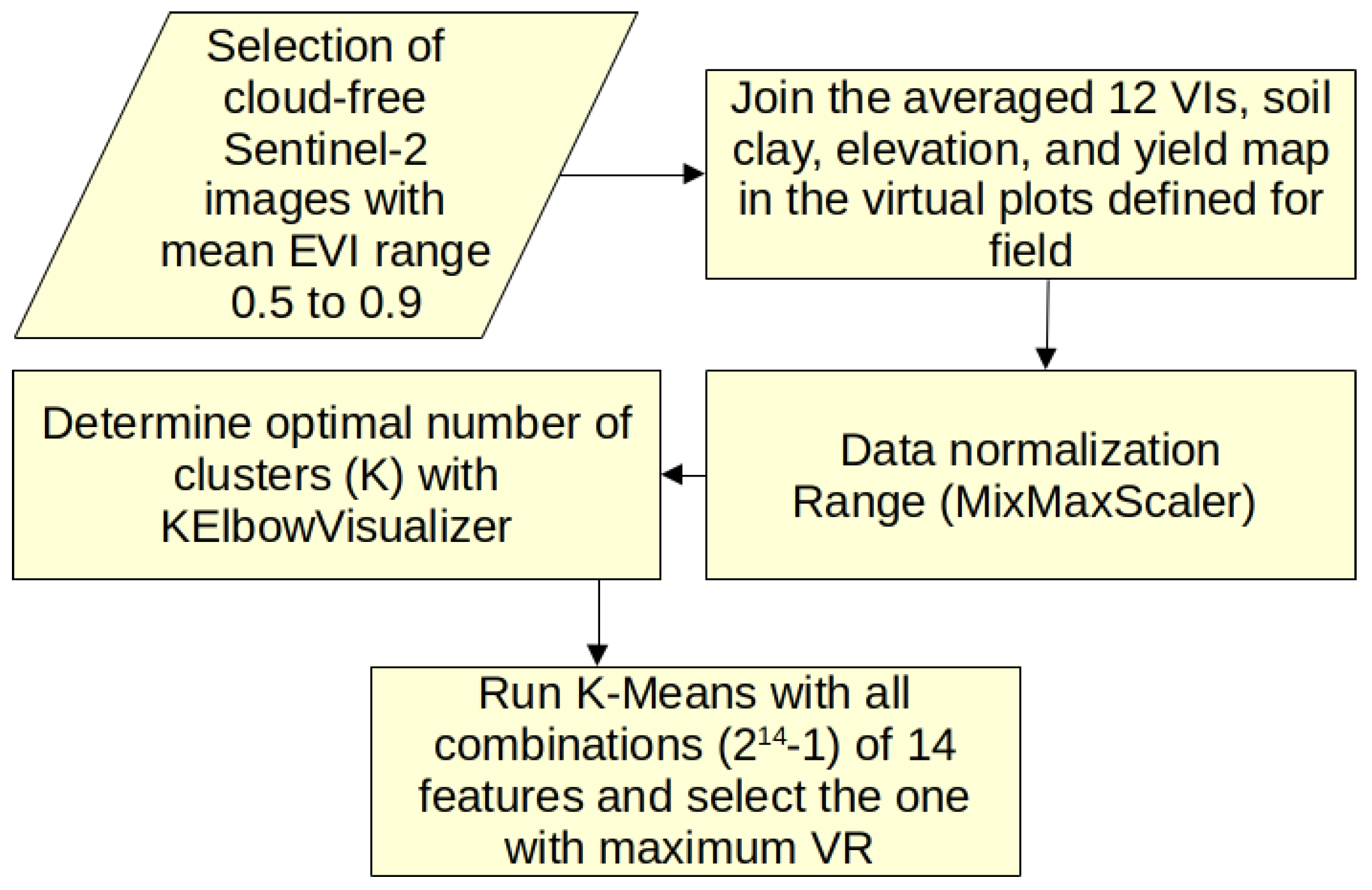
A step-by-step flowchart (Figure 4) was created to illustrate the entire methodology for delineating MZs.

2.3. Statistical Analysis of Population Effect on Cotton Yield

The primary research question addressed was: Does variation in plant population density within a specified range affect cotton yield? To investigate this question while accounting for spatial variability in heterogeneous production fields, a single-plot approach using a Latin square (LS) design was employed. Five production fields were sown with four target population densities, centered around the regional standard density, informed by farmer expertise and seed company recommendations. Each field was systematically arranged to incorporate plant density variation, with the analytical focus on estimating the effect of population density in typically heterogeneous fields. Given the quantitative nature of the controlled variable (population density) and the limited number of target densities, linear regression models were fitted in SAS (version 9.4) to evaluate the relationship with cotton yield. For each target plot, linear regression models were fitted to data from $4\times 4$ LS designs, selected to include the target plot and allowing up to four missing plots to accommodate irregular field shapes. The slopes from these models were combined in Python to classify the density effect as negative ($-1$), positive ($+1$), or non-significant (0), based on their sign and significance ($p\le 0.05$, F-test). The relationship between these classified effects and the predefined management zones was evaluated using statistical routines available in R software (version 4.4.3) [19] by analyzing their joint and marginal distributions. All models adjusted for spatial variation, with significance assessed at $\alpha =0.05$. Details of each step are provided in the following subsections.

2.3.1. Latin Square Selection

To evaluate the effect of plant population density on cotton yield, each field was divided into a grid with dimensions $n_r=max\left(\mathrm{row}\right)$ and $n_c=max\left(\mathrm{column}\right)$, with four target population density (TarPop, plants m⁻¹) assigned in a LS design. For each grid point $(R,C)$, where $R=1,\dots ,n_r$ and $C=1,\dots ,n_c$, a $4\times 4$ subgrid (rows $(R-1,R+2]$, columns $(C-1,C+2]$) was extracted and assigned a unique identifier R_C, in a dataset column LS. Subgrids with at least 12 plots ($n_{\mathrm{plot}}\ge 12$), allowing for the absence of up to one row or column to accommodate geometrically irregular fields, were retained as LSs. Each plot within a subgrid was assigned a unique identifier formatted as R_C, stored in the dataset column IDplot. The algorithm produces a dataset LSs containing LS subgrids (with columns row, column, TarPop, PopApl, Yield, IDplot, nplot referring to target and applied plant density, plot ID and number of plots in the subgrid) and a dataset LSPlotList storing subgrid identifiers in column LS and their comma-separated plot lists in column Plots. The selection process is detailed in Algorithm A1, Appendix A.

2.3.2. Regression Analysis

For each LS, cotton yield (Y, kg ha⁻¹) was modeled as a function of the applied plant density (PopApl, plants m⁻¹), centered on the overall mean of the field, using a generalized linear mixed model (GLMM) implemented in the GLIMMIX procedure of SAS [20]. The model was fitted using restricted pseudo-likelihood (method = RSPL) with the linear predictor:

$$\eta =X\beta ,$$

(3)

where X is the design matrix for plant density, and $\beta$ is the regression slope, specified without an intercept (noint). Spatial heterogeneity was accounted for by including random effects for row and column, modeled as described by [21]:

$$Y=X\beta +Z\gamma +ϵ,$$

(4)

where Y is the yield vector, Z is the design matrix for random effects, $\gamma \sim N(0,G)$ represents row and column effects, and $ϵ\sim N(0,R)$ is the residual error. The covariance matrix G was specified as diagonal to account for spatial heterogeneity by allowing independent random effects for rows and columns, improving the precision of $\widehat{\beta }$, while R was diagonal with homoscedastic residual errors to maintain a simple residual structure. Parameter estimates were extracted to ParEstLS using SAS Output Delivery System (ODS output). A data step added a column Recp to ParEstLS, assigning $-1$ for a significant ($p\le 0.05$, F-test) negative slope, 1 for a significant positive slope, and 0 otherwise. The Recp value represents the predicted effect of increasing plant density by one plant per meter above the overall mean of the field.

2.3.3. Combining Multiple Models for Density Effect Classification

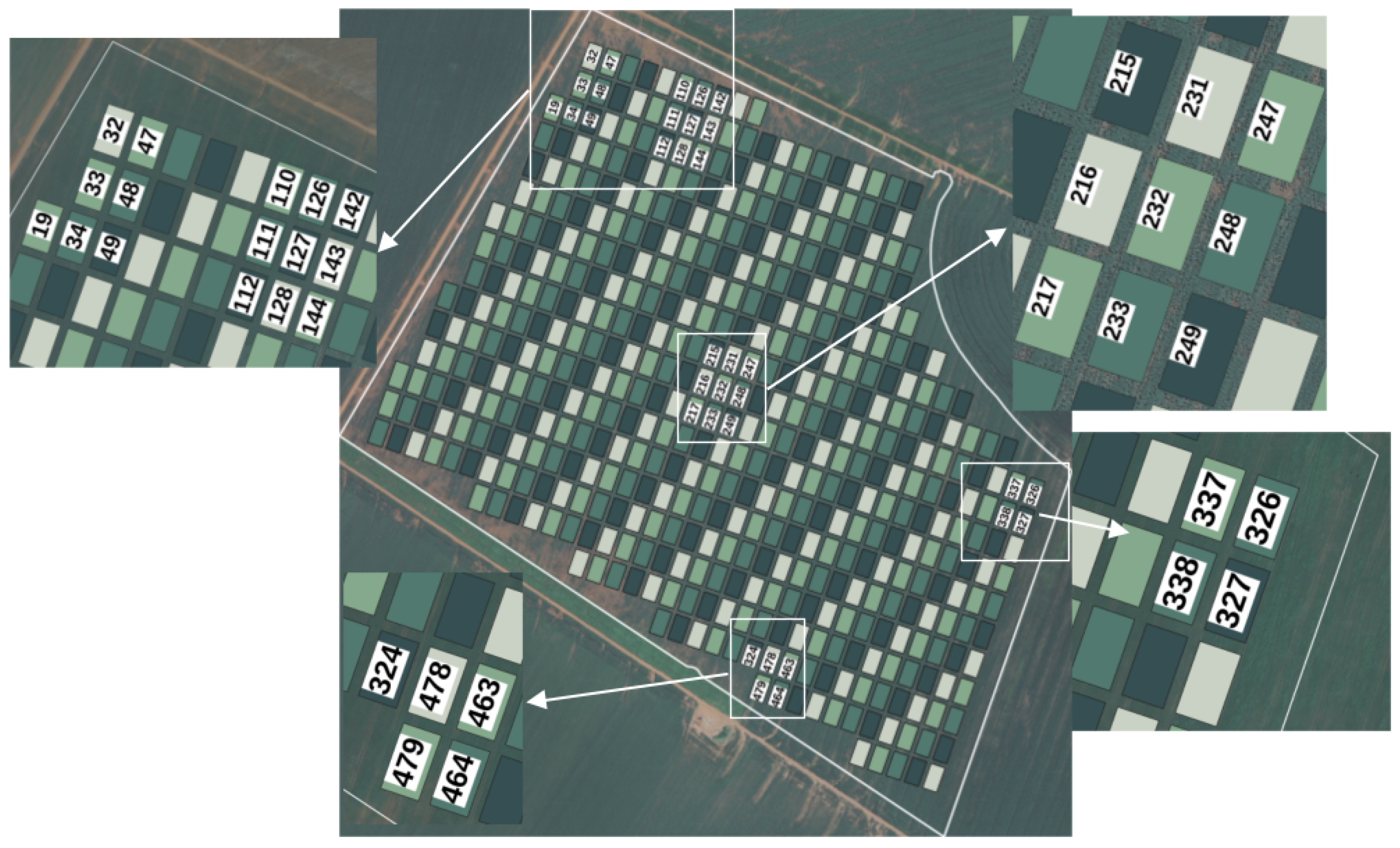
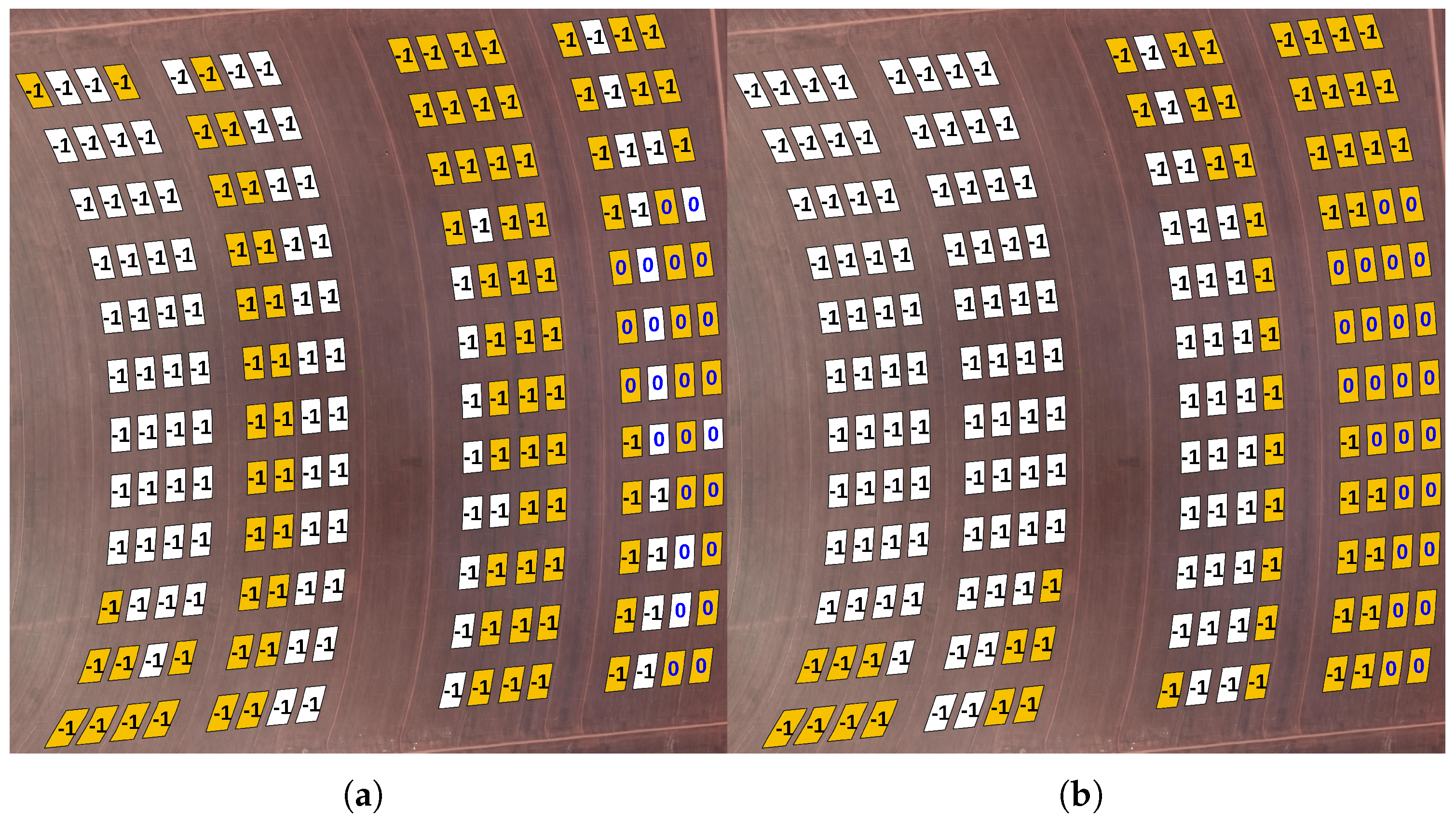
Each plot within a $4\times 4$ LS is included in multiple regression models, each yielding a potentially different predicted density effect class (Recp, $-1$, $+1$, or 0). To assign a single density effect class to each plot, two ensemble approaches were employed. The first approach used majority voting Algorithm A2 of Recp values from all models containing the plot. The second approach extended the first by including Recp values from models of its immediate neighbors, as illustrated in Figure 5. Ties were resolved by the sign of the sum of all Recp values. The classification process is detailed in the three-stage algorithmic pipeline (Algorithm A3). Alternative variations of these criteria were explored, including one weighting votes by the proportion of plots in the LS relative to 16, and another using non-centered plant population density with standard linear regression models. These variations were disregarded because most plots had similar density effect classes, despite differing class proportions, and exhibited weaker association with management zones, as described in the subsequent Section 2.3.4.

2.3.4. Association Analysis Between Predicted Classes and Management Zones

To evaluate the association between predicted plant density class effects and management zones, chi-square tests of independence were applied to contingency tables (MZ × Cl), and Cramér’s V was computed to assess the strength of association. The chi-square test of independence, implemented via the chisq.test function in the stats package [19], was used as the default method, with the test statistic calculated as:

$${\chi }^2=\sum {\displaystyle \frac{{(O_{ij}-E_{ij})}^2}{E_{ij}}},$$

(5)

where $O_{ij}$ denotes observed frequencies and $E_{ij}$ denotes expected frequencies, computed from the marginal totals of the contingency table. The associated p-value is derived from the chi-square distribution with $(r-1)(c-1)$ degrees of freedom, where r and c are the number of rows and columns in the contingency table, respectively.

To ensure the validity of the chi-square test, expected frequencies ($E_{ij}$) were evaluated. The chi-square test was deemed appropriate when no expected frequency was less than 1 and at most 20% of cells had expected frequencies below 5 (i.e., at most one cell for $3\times 2$ tables and none for $2\times 2$ tables). If these conditions were not met, Fisher’s exact test, implemented via the fisher.test function in the stats package, was applied. Fisher’s exact test computes an exact p-value based on the hypergeometric distribution, suitable for tables with small frequencies or sample sizes. For cases where Class contained only one category, no independence test was performed.

For exploratory purposes, when Fisher’s exact test was used due to inadequate expected frequencies, the chi-square test statistic and p-value were computed and reported as exploratory results, with a caveat that they were not reliable for inference due to assumption violations.

Expected frequencies for all contingency tables were calculated and recorded to justify the choice between chi-square and Fisher’s exact tests, using:

$$E_{ij}={\displaystyle \frac{R_i·C_j}{n}},$$

(6)

where $R_i$ is the row total for row i, $C_j$ is the column total for column j, and n is the total sample size.

The strength of association between MZ and Cl was quantified using Cramér’s V, calculated via the assocstats function in the vcd package [22], as:

$$V=\sqrt{{\displaystyle \frac{{\chi }^2}{n·min(r-1,c-1)}}}.$$

(7)

The effect of plant population density (PopApl) on cotton yield was studied for plots categorized by management zones (MZ) and density effect classes (Cl) using linear regression models, requiring a minimum of eight plots per model, based on the framework in Section 2.3.2, except with non-centered PopApl and an intercept.

3. Results

3.1. Management Zones

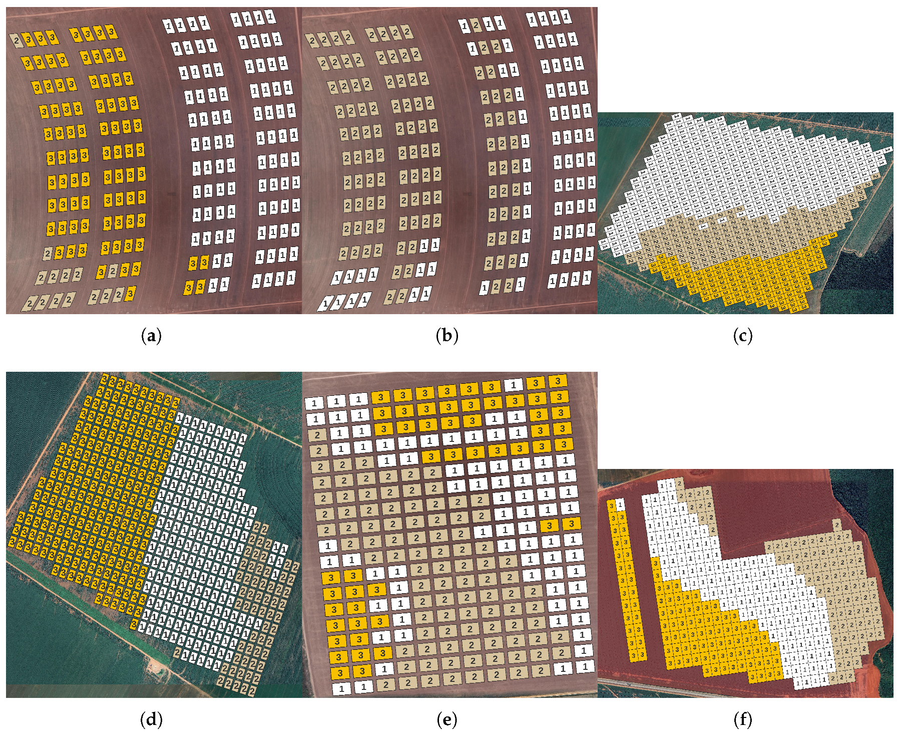
Figure 6 displays the three MZs delineated for all fields, except field A (23/24), which had only two. Although three MZs yielded a higher VR for field A (23/24), the two-MZ delineation is presented here due to its stronger correlation with seed population. The selected input attributes that resulted in the highest VR and respective SW for each field is presented in

Table 6. Clustering parameters, quality evaluation metrics of clustering results, average yield values for the entire field and for each MZ, along with the corresponding number of grid cells.

Field	Attributes	VR %	SW	Yield (kg ha−1)
				Field	MZ1	MZ2	MZ3
A 22/23	CIRE, CVI, Elevation, NDRE	60.3	0.748	4424	4662 (186)	2732 (19)	4087 (32)
A 23/24 (2 MZs)		19.8	0.417	4936	4795 (74)	5025 (118)	-
A 23/24 (3 MZs)		32.8	0.578	4936	5179 (55)	4852 (96)	4809 (41)
B	Clay, GNDVI	41.2	0.443	4627	4793 (39)	4501 (168)	4287 (129)
C	Elevation, GNDVI, PSRI	34.4	0.519	4529	4752 (199)	4457 (59)	4348 (221)
D	EVI, GNDVI, NDVI, PSRI, RVI	67.1	0.545	3449	3397 (79)	3798 (97)	2878 (52)
E	CVI, DVI, Elevation, GNDVI	49.2	0.310	5159	5043 (136)	5530 (88)	4993 (100)

.

3.2. Population Density Effect Classes

Using multiple regression models to assess plot responses to plant population density (PopApl), as described in Section 2.3.2, reduces the likelihood of misclassification. In this study, two classifiers, corresponding to the ensemble approaches in Section 2.3.3, consistently assigned the same density effect class to most plots, with differing class proportions between methods. Each model assigned a density effect class (Recp, $-1$, $+1$, or 0), and the final class (Cl) was determined by MV (majority voting of Recp values from models containing the plot) or NEMV (neighbor-enhanced majority voting, including Recp values from adjacent plots’ models), defined in Algorithm A4. Each plot was included in 1–16 models for field B, 2–16 for field C, and 3–16 for fields A, D, and E, depending on its position and the field’s geometry. Classifier MV used information from these models, while NEMV used at least 12 models per plot for field B, 15 for field C, and 21 for fields A, D, and E, with a maximum of 144 models across all fields.

All five fields showed no positive response to increasing plant density above the field averages in the 2023/2024 crop season, with negative responses observed in 84% of plots in field A, 17% in field B, 31% in field C, and 3% in field E (

Table 7. Percentages of plots by plant density class, chi-square test statistics (${\chi }_c^2$), p-values from chi-square and Fisher’s exact tests for independence, Cramer’s V association strength ($V_c$), number of management zones (nMZ), and classifiers across different cultivation fields.

				Effect Class			Independency				Cramer’s V
Field	nMZ	nPlot	Classifier	−1	0	1	${\mathbf{\chi }}_{\mathbf{c}}^{\mathbf{2}}$	${\mathit{p}}_{{\mathbf{\chi }}^{\mathbf{2}}}$	${\mathit{p}}_{\mathrm{Fisher}}$	Interpretation	${\mathit{V}}_{\mathit{c}}$	Strength
A a	2	192	MV	-	33%	67%	1.18	$3\times {10}^{-1}$	-	Non-significant	0.08	Negligible
	2	192	NEMV	-	31%	69%	0.95	$3\times {10}^{-1}$	-	Non-significant	0.07	Negligible
	3	192	MV	-	33%	67%	10.42	$6\times {10}^{-3}$	-	Significant	0.23	Moderate
	3	192	NEMV	-	31%	69%	11.08	$3\times {10}^{-3}$	-	Significant	0.24	Moderate
A b1	2	192	MV	84%	16%	-	0.99	$3\times {10}^{-1}$	-	Non-significant	0.07	Negligible
	2	192	NEMV	87%	13%	-	2.55	$1\times {10}^{-1}$	-	Non-significant	0.12	Weak
	3	192	MV	84%	16%	-	32.65	$8\times {10}^{-8}$	-	Significant	0.41	Relatively strong
	3	192	NEMV	87%	13%	-	36.62	$1\times {10}^{-8}$	-	Significant	0.44	Relatively strong
A b2	2	192	MV	84%	16%	-	37.85	$8\times {10}^{-10}$	-	Significant	0.44	Relatively strong
	2	192	NEMV	87%	13%	-	42.01	$9\times {10}^{-11}$	-	Significant	0.47	Relatively strong
	3	192	MV	84%	16%	-	32.65	$8\times {10}^{-8}$	-	Significant	0.41	Relatively strong
	3	192	NEMV	87%	13%	-	36.62	$1\times {10}^{-8}$	-	Significant	0.44	Relatively strong
B b2	2	688	MV	17%	83%	-	30.04	$4\times {10}^{-8}$	-	Significant	0.20	Weak
	2	688	NEMV	17%	83%	-	35.58	$3\times {10}^{-9}$	-	Significant	0.23	Moderate
	3	688	MV	17%	83%	-	57.30	$4\times {10}^{-13}$	-	Significant	0.29	Moderate
	3	688	NEMV	17%	83%	-	62.47	$3\times {10}^{-14}$	-	Significant	0.30	Moderate
C b2	2	479	MV	30%	70%	-	3.44	$6\times {10}^{-2}$	-	Non-significant	0.08	Negligible
	2	479	NEMV	31%	69%	-	7.98	$5\times {10}^{-3}$	-	Significant	0.13	Weak
	3	479	MV	30%	70%	-	47.85	$4\times {10}^{-11}$	-	Significant	0.32	Moderate
	3	479	NEMV	31%	69%	-	58.65	$2\times {10}^{-13}$	-	Significant	0.35	Moderate
D b2	3	228	MV	-	100%	-	-	-	-	-	-	-
	3	228	NEMV	-	100%	-	-	-	-	-	-	-
E b2	3	297	MV	3%	97%	-	27.47	$3\times {10}^{-6}$	$1\times {10}^{-6}$	Significant	0.30	Moderate
	3	297	NEMV	3%	97%	-	24.34	$5\times {10}^{-6}$	$1\times {10}^{-5}$	Significant	0.29	Weak

^a Crop season 2022/2023, MZ 2022/2023; ^b1 Crop season 2023/2024, MZ 2022/2023; ^b2 Crop season 2023/2024, MZ 2023/2024.

and 

Table 8. Joint and marginal distributions of plot counts (n) with percentages, average population density (PopApl), yield (kg⁻¹), and clay content (%) across MZs and effect classes (Cl). Marginal distributions are denoted by ∑ for MZ and Cl.

Field	Cl	n				%				PopApl				Yield				Clay
		MZ				MZ				MZ				MZ				MZ
		1	2	3	∑	1	2	3	∑	1	2	3	∑	1	2	3	∑	1	2	3	∑
A a	0	19	7	34	60	24%	78%	33%	31%	11.1	12.0	12.0	11.7	4606	4272	4682	4520	46	24	37	36
	1	60	2	70	132	76%	22%	67%	69%	10.6	11.5	12.1	11.4	4483	5034	4805	4774	55	44	37	45
	∑	79	9	104	192	41%	5%	54%	−	10.9	11.7	12.1	11.5	4544	4653	4743	4646	50	34	37	43
A b1	$-1$	55	8	104	167	70%	89%	100%	87%	11.8	11.2	11.7	11.6	4737	5100	5073	4970	51	25	37	38
	0	24	1	0	25	30%	11%	0%	13%	11.6	14.4	−	13.0	4723	4359	−	4541	57	51	−	54
	∑	79	9	104	192	41%	5%	54%	−	11.7	12.8	11.7	11.7	4730	4729	5073	4930	54	38	37	43
A b2	$-1$	114	53	−	167	100%	68%	−	87%	11.7	11.7	−	11.7	5058	4760	−	4909	38	48	−	43
	0	0	25	−	25	0%	32%	−	13%	11.7	11.7	−	11.7	−	4708	−	4708	−	57	−	57
	∑	114	78	−	192	59%	41%	−	−	11.7	11.7	−	11.7	5058	4734	−	4930	38	52	−	43
B b2	$-1$	102	0	13	115	26%	0%	10%	17%	8.4	−	8.0	8.2	4838	−	4131	4485	63	−	28	45
	0	289	168	116	573	74%	100%	90%	83%	8.1	8.1	8.1	8.1	4774	4500	4306	4527	59	48	35	47
	∑	391	168	129	688	57%	24%	19%	−	8.3	8.1	8.0	8.1	4806	4500	4219	4626	61	48	31	52
C b2	$-1$	95	0	52	147	48%	0%	24%	31%	9.1	−	9.1	9.1	4717	−	4460	4588	32	−	39	36
	0	104	59	169	332	52%	100%	76%	69%	9.3	8.5	9.0	8.9	4774	4453	4321	4516	29	21	57	36
	∑	199	59	221	479	42%	12%	46%	−	9.2	8.5	9.1	9.1	4745	4453	4390	4529	31	21	48	40
D b2	∑	79	97	52	228	35%	43%	23%		10.2	10.6	10.4	10.4	3386	3786	2853	3435	14	17	13	15
E b2	$-1$	0	0	9	9	0%	0%	12%	3%	−	−	10.7	10.7	−	−	5102	5102	−	−	55	55
	0	135	87	66	288	100%	100%	88%	97%	10.8	10.8	10.7	10.8	5119	5130	5112	5121	38	32	47	39
	∑	135	87	75	297	45%	29%	25%	−	10.8	10.8	10.7	10.8	5119	5130	5107	5120	38	32	51	39

^a Crop season 2022/2023, MZ 2022/2023; ^b1 Crop season 2023/2024, MZ 2022/2023; ^b2 Crop season 2023/2024, MZ 2023/2024.

). In Table 7, the strong and moderate Cramer’s V values are essential for determining if the effect of increasing seed rate is negative, positive, or indifferent. These results suggest that, under the weather conditions of that crop season and plant sowing dates, reducing plant density would not negatively impact cotton yield and could potentially increase it. Field A was assessed in two consecutive crop seasons (2022/2023 and 2023/2024), allowing comparison of responses between seasons. In 2022/2023, approximately 31% of plots were classified as 0 and 69% as $+1$, in contrast to the 2023/2024 season, where all plots classified as 0 in 2022/2023 shifted to $-1$, and 19% of plots classified as $+1$ shifted to $-1$. Given that the sowing density was consistent with the average plant densities of 11.5 and 11.7 plants per meter in 2022/2023 and 2023/2024, respectively, the potential yield gain from adding plants above 11.5 in 2022/2023 is not guaranteed due to unpredictable weather conditions, which could lead to losses in seed and yield.

3.3. Associations Between Management Zones and Density Effect Classes

This study’s experimental design allowed for a detailed comparison of plant density effects at the plot level against those across MZs. MZs, typically delineated using yield-correlated VIs, may not fully account for all production-limiting factors, such as soil variability. We therefore analyzed the joint distribution of plant density effect classes ($\mathtt{Cl}$: $-1$, $+1$, or 0) and MZs to assess their effectiveness in identifying responsive areas. This evaluation explores whether MZs can simplify the prescription of optimal plant densities, thereby stabilizing yield potential. Such an approach refines precision agriculture by enabling targeted management strategies that optimize cotton yield while minimizing resource inputs.

The association between population density effect classes and MZs was analyzed using the MV and NEMV classifiers described in Section 2.3.3. For Field A in the 2022/2023 crop season (denoted by A^a in Table 7), the association with two MZs was not statistically significant, indicating no clear pattern between density effect classes and MZs (approximately equal distribution of classes within each MZ). In contrast, the association with three MZs was highly significant (Table 7), with a Cramer’s $V_c$ value indicating a moderate relationship, suggesting that three MZs better captured variations in plant density responses. For Field A in the 2023/2024 crop season, MZs were constructed using data up to the 2022/2023 (A^b1) and 2023/2024 (A^b2) crop seasons. The association for A^b2 was relatively strong, even with two MZs, as shown in Table 7. This improvement likely results from incorporating additional data into the vegetation index series, refining MZ definitions.

For Fields B, C, D, and E in the 2023/2024 crop season, independence tests revealed highly significant associations with moderate $V_c$ values, indicating that MZs effectively distinguished areas with varying plant density responses. Based on these findings, we selected the number of MZs and classifier with the strongest association, as shown by the highest $V_c$ value (highlighted in bold in Table 7). This selection identified characteristics, such as applied density and clay content, contributing to heterogeneous responses within management zones. These results highlight the importance of choosing an appropriate number of MZs to optimize plant density management, enabling farmers to target high-response zones for improved cotton yield and resource efficiency.

3.4. Exploring Plant Density Effect Across Effect Classes and Management Zones

The percentage of plots in each class across each management zone, shown in Table 8, was calculated as $\%n_{ij}={\displaystyle \frac{n_{ij}}{n_{.j}}}$, where $n_{ij}$ is the plot count in class i ($i\in \{-1,0,1\}$) within MZ j ($j\in \{1,2,3\}$), $n_{.j}$ is the total plot count in MZ j, and $\%n_{ij}$ represents the percentage of plots in Cl i within MZ j. This summary in Table 8 supports the interpretation of associations in Table 7.

For field A, crop season 2022/2023 (A^a), Table 7 shows a weaker association, with 76% of plots in MZ 1 (50% clay content) and 67% in MZ 3 (37% clay content) classified as class 1 (positive effect), and 78% in MZ 2 (24% clay content) classified as class 0 (no significant effect), suggesting that clay content differences did not strongly drive the distribution of effect classes across MZs. This apparent inconsistency may stem from the low uniformity of the average applied seed density (PopApl), which differs by 1.5 seeds per meter in favor of MZ 3 (12.1 for class 1 in A^a, compared to 10.6 for class 1 in MZ 1). This variability limits the ability to isolate the contributions of PopApl and Clay. The regression models in

Table 9. Regression models for plots categorized by management zones (MZ) and effect classes (Cl). Includes denominator degrees of freedom (DDF) of the F-test for population density (P, plants m⁻¹), corresponding p-values (p), and marginal distributions (∑).

		MZ1			MZ2			MZ3			∑
Field	Cl	Model	DDF	$\mathit{p}$	Model	DDF	$\mathit{p}$	Model	DDF	$\mathit{p}$	Model	DDF	$\mathit{p}$
A a	0	$\mathbf{Y}=\mathbf{3900}+\mathbf{60}.\mathbf{2}$P	9	$\mathbf{2}\times {\mathbf{10}}^{-\mathbf{2}}$	−	−	−	$Y=4835-2.2P$	26	$9\times {10}^{-1}$	$Y=4416+14.7P$	38	$4\times {10}^{-1}$
	1	Y $=3915+68.4$P	45	$\mathbf{6}\times {\mathbf{10}}^{-\mathbf{10}}$	−	−	−	$\mathbf{Y}=\mathbf{4225}+\mathbf{49}.\mathbf{1}$P	47	$1\times {10}^{-4}$	$\mathbf{Y}=\mathbf{4043}+\mathbf{56}.\mathbf{3}\mathbf{P}$	104	$\mathbf{2}\times \mathbf{10}-\mathbf{11}$
	∑	Y $=3856+65.2$P	61	$\mathbf{3}\times {\mathbf{10}}^{-\mathbf{10}}$	$Y=6562-178.5P$	7	$6\times {10}^{-2}$	Y $=4334+39.4$P	84	$\mathbf{3}\times {\mathbf{10}}^{-\mathbf{4}}$	Y $=4126+45.2$P	167	$\mathbf{4}\times {\mathbf{10}}^{-\mathbf{6}}$
A b1	$-1$	Y $=5446-53.6$P	34	$\mathbf{1}\times {\mathbf{10}}^{-\mathbf{7}}$	Y $=6399-119.7$P	2	$\mathbf{4}\times {\mathbf{10}}^{-\mathbf{3}}$	Y $=5737-58.3$P	82	$\mathbf{1}\times {\mathbf{10}}^{-\mathbf{13}}$	Y $=5611-57.6$P	140	$\mathbf{8}\times {\mathbf{10}}^{-\mathbf{21}}$
	0	$Y=4689+2.9P$	22	$9\times {10}^{-1}$	−	−	−	−	−	−	$Y=4699-0.1P$	12	$1\times {10}^0$
	∑	Y $=5190-34$P	54	$\mathbf{4}\times {\mathbf{10}}^{-\mathbf{3}}$	Y $=6352-120.2$P	2	$\mathbf{3}\times {\mathbf{10}}^{-\mathbf{3}}$	Y $=5737-58.3$P	82	$\mathbf{1}\times {\mathbf{10}}^{-\mathbf{13}}$	Y $=5515-49.8$P	164	$\mathbf{1}\times {\mathbf{10}}^{-\mathbf{14}}$
A b2	$-1$	Y $=5729-57.6$P	91	$\mathbf{9}\times {\mathbf{10}}^{-\mathbf{15}}$	Y $=5488-53.1$P	30	$\mathbf{2}\times {\mathbf{10}}^{-\mathbf{7}}$	−	−	−	Y $=5611-57.6$P	140	$\mathbf{8}\times {\mathbf{10}}^{-\mathbf{21}}$
	0	−	−	−	$Y=4699-0.1P$	12	$1\times {10}^0$	−	−	−	$Y=4699-0.1P$	12	$1\times {10}^0$
	∑	Y $=5729-57.6$P	91	$\mathbf{9}\times {\mathbf{10}}^{-\mathbf{15}}$	Y $=5273-34.7$P	51	$\mathbf{5}\times {\mathbf{10}}^{-\mathbf{3}}$	−	−	−	Y $=5515-49.8$P	164	$\mathbf{1}\times {\mathbf{10}}^{-\mathbf{14}}$
B b2	$-1$	Y $=5245-43.1$P	69	$\mathbf{5}\times {\mathbf{10}}^{-\mathbf{8}}$	−	−	−	Y $=4488-39.4$P	4	$\mathbf{2}\times {\mathbf{10}}^{-\mathbf{3}}$	Y $=5072-42.6$P	79	$\mathbf{2}\times {\mathbf{10}}^{-\mathbf{9}}$
	0	$Y=4880-1.2P$	232	$8\times {10}^{-1}$	$Y=4644-9.4P$	126	$1\times {10}^{-1}$	Y $=4481-17.6$P	82	$\mathbf{1}\times {\mathbf{10}}^{-\mathbf{2}}$	$Y=4734-6.7P$	499	$7\times {10}^{-2}$
	∑	Y $=4988-14.3$P	333	$\mathbf{8}\times {\mathbf{10}}^{-\mathbf{4}}$	$Y=4644-9.4P$	126	$1\times {10}^{-1}$	Y $=4500-20.5$P	95	$\mathbf{3}\times {\mathbf{10}}^{-\mathbf{3}}$	Y $=4792-13.9$P	613	$\mathbf{2}\times {\mathbf{10}}^{-\mathbf{5}}$
C b2	$-1$	Y $=5100-43.9$P	64	$\mathbf{6}\times {\mathbf{10}}^{-\mathbf{10}}$	−	−	−	Y $=4706-32.1$P	30	$\mathbf{6}\times {\mathbf{10}}^{-\mathbf{5}}$	Y $=4960-37.3$P	110	$\mathbf{4}\times {\mathbf{10}}^{-\mathbf{11}}$
	0	$Y=4936-14.4P$	72	$7\times {10}^{-2}$	$Y=4385+8.1P$	47	$7\times {10}^{-1}$	Y $=4506-15.5$P	141	$\mathbf{3}\times {\mathbf{10}}^{-\mathbf{2}}$	$Y=4639-10.7P$	283	$8\times {10}^{-2}$
	∑	Y $=4986-27.4$P	165	$\mathbf{5}\times {\mathbf{10}}^{-\mathbf{6}}$	$Y=4385+8.1P$	47	$7\times {10}^{-1}$	Y $=4565-19.7$P	192	$\mathbf{1}\times {\mathbf{10}}^{-\mathbf{3}}$	Y $=4717-19.1$P	429	$\mathbf{8}\times {\mathbf{10}}^{-\mathbf{5}}$
D b2	∑	Y $=3676-29$P	68	$\mathbf{4}\times {\mathbf{10}}^{-\mathbf{2}}$	$Y=3911-12.1P$	85	$3\times {10}^{-1}$	$Y=2781+5.4P$	35	$7\times {10}^{-1}$	$Y=3504-6.6P$	213	$6\times {10}^{-1}$
E b2	$-1$	−	−	−	−	−	−	$Y=5083+1.8P$	4	$5\times {10}^{-1}$	$Y=5083+1.8P$	4	$5\times {10}^{-1}$
	0	$Y=5121-0.1P$	116	$8\times {10}^{-1}$	$Y=5119+0.9P$	65	$2\times {10}^{-1}$	Y $=5097+1.6$P	52	$\mathbf{5}\times {\mathbf{10}}^{-\mathbf{2}}$	$Y=5118+0.4P$	245	$3\times {10}^{-1}$
	∑	$Y=5121-0.1P$	116	$8\times {10}^{-1}$	$Y=5119+0.9P$	65	$2\times {10}^{-1}$	$Y=5099+1.3P$	61	$8\times {10}^{-2}$	$Y=5118+0.4P$	252	$3\times {10}^{-1}$

^a Crop season 2022/2023, MZ 2022/2023; ^b1 Crop season 2023/2024, MZ 2022/2023; ^b2 Crop season 2023/2024, MZ 2023/2024. Bold equation models represent significant slope ($p\le 0.05$).

for MZ 1, class 1, show a significant yield increase of 68.5 kg ha⁻¹ per additional cotton plant in the interval [8.5, 13.0], compared to 49.1 kg ha⁻¹ in MZ 3, in the interval [8.5, 15.0]. For all data in these MZs, the estimated increase per added plant is 65.5 kg ha⁻¹ in MZ 1 and 39.4 kg ha⁻¹ in MZ 3, over the same intervals. For MZ 2, with only nine plots (seven at 24% clay content in class 0 and two at 44% in class 1), the regression model yields a p-value of 6%, close to the 5% cutoff. This model indicates a yield decrease of 178.5 kg ha⁻¹ per plant added, strongly influenced by the low clay content of seven plots. In summary, for A^a, the single plot approach identified plots with greater yield responses to plant density variations, while regression models fitted for each MZ provided consistent management recommendations with varying slopes.

The influence of accurate sowing and well-defined MZs strengthens the relationship between plant density effect classes and yield responses in field A’s 2023/2024 crop season. Compared to the variable seed density and weaker associations in 2022/2023 (A^a), the block A^b1, using prior MZ, shows a stronger association, supported by more uniform average plant density across MZ (Table 8, showing plot class distributions by MZ). In A^b2, with MZ defined using historical vegetation index series up to 2023/2024, sowing was uniformly 11.7 plants per meter, yielding the highest association among all cases. Here, 100% of MZ 1 plots and 68% of MZ 2 plots were classified as having significant yield loss (class $-1$) for added seeds in the [9.0, 14.4] plants per meter interval. Regression models in (Table 9) estimate that adding one plant per meter in the studied plant density range reduces yield by 58.6 kg ha⁻¹ in MZ 1 and 35.6 kg ha⁻¹ in MZ 2. The yield loss in Zone 1 is 23 kg ha⁻¹ higher, with MZ 1 at 38% clay and MZ 2 at 52%. The model for the 68% of MZ 2 plots classified as $-1$ estimates a loss of 53.1 kg ha⁻¹, closely matching MZ 1’s 58.6 kg ha⁻¹ and the 57.6 kg ha⁻¹ for all class $-1$ plots, confirming the single plot approach’s accuracy in identifying plots with significant negative yield responses. Plots in MZ 2 with no significant response (class 0, 57% Clay) had the highest clay content, while those with losses (48% in class $-1$, 52% overall in $MZ$ 2) had lower clay content (Table 8). In summary, for both seasons, the single plot approach in joint distributions consistently identified plots with negative yield responses to plant density increases, while MZ-level models provided similar management recommendations. A^b2’s updated MZ definitions yield the most robust associations, though differences in regression slopes reflect varying clay content influences (Figure 7).

Fields B and C, with average plant densities of 8.1 and 9.1 plants per meter in the 2023/2024 crop season, had 17% and 31% of their plots, respectively, showing significant negative yield responses to plant density increases in the sowing intervals [5.3, 11.0] and [6.1, 13.0] (Table 8). In field B, MZ 1—comprising 57% of plots with an average clay content of 59% and 8.1 plants per meter—had 74% of plots classified as class 0 (no significant response), with a non-significant regression slope (Table 9). In field C, MZ 3, the largest zone with 46% of plots and 57% clay content, had 76% of plots classified as class 0 but showed a significant yield loss of 15.5 kg ha⁻¹ per plant added ($p\le 0.05$). Field B’s MZ 2 (24% of plots, all class 0) and field C’s MZ 1 (42% of plots, 58% class 0) had intermediate clay contents of 48% and 29%, respectively, with non-significant regression slopes. The single plot approach more accurately identified yield losses in subareas of these MZ, typically correlated with lower clay content, while models fitted across all plots suggest optimal plant densities are near the lower bounds of the sowing intervals (5.3 for B, 6.1 for C).

Field D, with an average of 10.5 plants per meter in the 2023/2024 crop season, showed no significant yield response to plant density variations in the sowing interval [8.0, 12.5], with 95% of plots classified as class 0 (Table 8). In field E, with a uniform average density of 10.7 plants per meter and clay content ranging from 32% to 55%, only 3% of plots exhibited significantly negative yield responses (class $-1$) in the interval [8.5, 13.0]. Regression models for field E’s MZ 1, with 55% clay content, showed a non-significant slope ($p\ge 0.05$), suggesting that the applied density may be near optimal or could be slightly reduced (Table 9). The single plot approach indicated that the few plots with negative responses in field E had lower clay content (32% to 40%), consistent with trends observed in fields A, B, and C, where lower clay content correlated with yield losses. Compared to the lower average densities of fields B (8.1 plants per meter) and C (9.1 plants per meter), field E’s higher density likely approaches the optimal range for its clay content profile.

4. Discussion

The findings of this research on optimizing cotton cultivation through VRS in commercial fields provide some insights, particularly when interpreted in the context of previous studies and the inherent complexities of real-world agricultural systems. The primary hypothesis that VRS can enhance crop performance by adapting seeding rates to field variability is strongly supported by the demonstrated ability of management zones (MZs) to identify areas that respond differently to plant density variations.

Previous research on cotton plant density presents contrasting findings, often influenced by environmental factors such as water availability. For instance, Kimura et al. [5] found no statistical differences in lint yield across various population densities in water-scarce environments, suggesting that lower final plant densities could optimize both yield and net return due to reduced seed costs. In contrast, Khan et al. [6] consistently reported that higher plant densities (e.g., 87,000 plants ha⁻¹) resulted in the highest seed cotton and lint yields, attributing this to greater biomass accumulation. Boyer et al. [7] identified a yield-maximizing seeding rate around 118,000 plants ha⁻¹, but crucially distinguished this from profit-maximizing rates, which were consistently lower (78,000 to 93,000 plants ha⁻¹, dependent on cotton and seed prices).

Our study’s results for the 2023/2024 crop season—showing no positive response to increasing plant density above the field averages and negative responses in a significant percentage of plots (e.g., 84% in Field A, 2023/2024)—align more closely with the perspective that lower densities can be optimal, especially for profit maximization or under specific environmental conditions. The comparison of Field A across two consecutive seasons (2022/2023 and 2023/2024) further highlights the influence of unpredictable weather conditions. A shift from a 69% positive response in 2022/2023 to predominantly negative responses in 2023/2024, despite consistent sowing densities, underscores the dynamic interplay between plant density, climate, and yield. This dynamic nature emphasizes the importance of site-specific adjustments that account for inter-seasonal variability.

The statistical correlation indicating that lower clay content is associated with yield reductions under higher plant densities should be interpreted within the framework of resource competition dynamics. Clay content serves as a fundamental determinant of soil physical and chemical properties, governing critical processes such as water retention, nutrient availability, and root development. In MZs characterized by lower clay content—such as MZ 1 (38% clay)—resource availability is inherently constrained; consequently, increased plant density exacerbates inter-plant competition, culminating in the observed negative yield responses. Quantitative evidence supports this interpretation: regression analyses revealed substantially greater yield reductions in low-clay zones (e.g., a 23 kg ha⁻¹ difference) compared with zones possessing higher clay content (e.g., MZ 2 at 52% clay), underscoring that resource scarcity amplifies the adverse effects of elevated plant population density.

The delineation of MZs proved to be an effective strategy, with significant associations found between MZs and plant density effect classes across most fields. Our findings consistently showed that lower clay content was correlated with yield losses at higher plant densities, particularly in fields A, B, and C. This provides strong evidence that soil properties, in conjunction with other factors, critically modulate the optimal seeding rate and yield response within different management zones.

Limitations emerged when transitioning from small, controlled research plots to large-scale, operational on-farm experimentation. Regarding spatial resolution, the methodology depended on input data of varying granularity: soil clay content maps were generated via kriging interpolation from sparsely distributed samples (one per 5 ha), while climate datasets—such as CHIRPS precipitation and ERA5-Land temperature—had relatively coarse spatial resolutions, ranging from approximately 5 km to 31 km. This disparity in spatial scale contrasts with the actual heterogeneity observed across the commercial fields, which are separated by distances of up to 19.2 km and exhibit substantial differences in accumulated rainfall.

With respect to climatic variability, the inter-seasonal shift in field A’s yield response (from 69% positive in 2022/2023 to predominantly negative in 2023/2024), despite constant sowing density, highlights that optimal seeding rates are highly sensitive to unpredictable weather conditions. Finally, the experimental design was necessarily constrained by the overarching objective of minimizing operational interference and relying exclusively on existing farm data. This constraint required a complex statistical framework, in which a single density-effect class for each plot was derived by combining outcomes from up to 16 regression models through ensemble methods (MV and NEMV), reflecting the inherent difficulty of isolating variables in heterogeneous commercial environments.

In context, the most substantial potential for profit improvement indicated by our results arises from the high proportion of plots exhibiting either no positive yield response (Class 0) or significant yield loss (Class −1) when plant density exceeded field averages during the 2023/2024 season. In field B, C, and D, Class 0 responses were observed in 83%, 69%, and 95% of plots, respectively. Under these conditions, VRS prescriptions would recommend reducing seeding rates toward the lower end of the tested range (e.g., 8.0 plants m⁻¹ in field D and 5.3 plants m⁻¹ in field B). In these non-responsive consistent with prior evidence that VRS improve resource-use efficiency and promotes sustainable production practices. This site-specific adjustment in seeding rates, which prevents excessive plant competition, is widely linked to higher input efficiency and overall sustainability.

Despite the demonstrated economic benefits of VRS, such as rapid payback periods, widespread adoption remains limited due to hurdles like initial investment. This research directly addresses this barrier by proposing a methodology for on-farm investigation that leverages already available data sources and minimizes interference with routine farm operations. By empowering farm managers to conduct their own site-specific experimentation, this approach facilitates the determination of the most profitable or highest-yielding seed populations tailored to unique field conditions, thereby promoting the broader integration of VRS into agricultural systems. Future research should continue to focus on improving spatial data precision and making these technologies even more accessible to further accelerate VRS adoption across diverse agricultural landscapes.

5. Conclusions

This study successfully established an enabling methodology for optimizing cotton cultivation through VRS in commercial on-farm settings. The approach prioritizes leveraging readily available farm data while minimizing operational interference, thereby addressing the critical gap between small, controlled experimental research plots and large-scale operational validation (fields ranging from 78 to 332 ha). By providing farm managers with a validated framework to conduct their own site-specific experimentation, this work directly contributes to advancing precision agriculture and empowering producers to determine the seed population that maximizes returns under their specific field conditions.

A key implication of the research is the validation of MZs as robust tools for guiding site-specific seeding decisions. Statistically significant associations were observed between MZs and plant population density effect classes across most experimental fields, demonstrating that MZs can effectively delineate areas that exhibit differentiated yield responses to seeding variation. Furthermore, the findings consistently showed that increasing plant density above field averages during the 2023/2024 season generally led to non-positive or negative yield responses, particularly in areas characterized by lower clay content. This strong evidence suggests that optimizing input use often requires reducing seeding rates in response to localized constraints. This approach is widely linked to higher input efficiency, promoting resource efficiency, and enhancing the economic viability and sustainability of cotton production by preventing yield losses caused by excessive inter-plant competition. The dynamic nature of yield responses, demonstrated by inter-seasonal variability, underscores the critical need for adaptive management strategies informed by historical field data.

Despite the methodology’s success in commercial implementation, several limitations must be acknowledged. The study relied on input data of varying granularity, specifically noting the disparity between the coarse spatial resolution of climate datasets (CHIRPS precipitation and ERA5-Land temperature, ranging from 5 km to 31 km) and the high heterogeneity observed across fields separated by up to 19.2 km. Additionally, the reliance on existing farm data constrained the experimental design, requiring a complex statistical framework involving ensemble regression methods to isolate variables in heterogeneous commercial environments.

Future research should focus on two main directions to accelerate the widespread adoption of VRS:

• Improving Spatial Data Precision: Continued effort is needed in developing and integrating high-resolution spatial data for key variables like soil properties and climate, which will enhance the accuracy and predictability of MZ delineation.
• Increasing Technology Accessibility: Further efforts must be made to simplify technology and data analysis requirements, making the methodology and subsequent VRS implementation more accessible to farm managers across diverse agricultural landscapes.

References

1. Anselmi, A.A.; Molin, J.P.; Bazame, H.C.; Corrêdo, L.d.P. Definition of Optimal Maize Seeding Rates Based on the Potential Yield of Management Zones. Agriculture 2021, 11, 911. [Google Scholar] [CrossRef]
2. Speranza, E.A.; Naime, J.d.M.; Vaz, C.M.P.; Santos, J.C.F.d.; Inamasu, R.Y.; Lopes, I.d.O.N.; Queirós, L.R.; Rabelo, L.M.; Jorge, L.A.d.C.; Chagas, S.d.; et al. Delineating Management Zones with Different Yield Potentials in Soybean–Corn and Soybean–Cotton Production Systems. AgriEngineering 2023, 5, 1481–1497. [Google Scholar] [CrossRef]
3. Šarauskis, E.; Kazlauskas, M.; Naujokienė, V.; Bručienė, I.; Steponavičius, D.; Romaneckas, K.; Jasinskas, A. Variable Rate Seeding in Precision Agriculture: Recent Advances and Future Perspectives. Agriculture 2022, 12, 305. [Google Scholar] [CrossRef]
4. Khan, A.; Kong, X.; Najeeb, U.; Zheng, J.; Tan, D.K.Y.; Akhtar, K.; Munsif, F.; Zhou, R. Planting Density Induced Changes in Cotton Biomass Yield, Fiber Quality, and Phosphorus Distribution under Beta Growth Model. Agronomy 2019, 9, 500. [Google Scholar] [CrossRef]
5. Kimura, E.; Adams, C.; DeLaune, P.B.; Ramirez, J.; Thapa, S. Effect of cotton population density on lint yield and fiber quality. Agrosyst. Geosci. Environ. 2024, 7, e20497. [Google Scholar] [CrossRef]
6. Khan, N.; Xing, F.; Feng, L.; Wang, Z.; Xin, M.; Xiong, S.; Wang, G.; Chen, H.; Du, W.; Li, Y. Comparative Yield, Fiber Quality and Dry Matter Production of Cotton Planted at Various Densities under Equidistant Row Arrangement. Agronomy 2020, 10, 232. [Google Scholar] [CrossRef]
7. Boyer, C.N.; Butler, S.; Raper, T.; Buschermohle, M.J.; Dodds, D.M.; Jones, A. Profit-Maximizing Planting Date and Seeding Rate for Upland Cotton in the Upper Mid-South. J. Cotton Sci. 2020, 24, 183–188. [Google Scholar] [CrossRef]
8. INPE/Terrabrasilis. Brazilian Biomes [Shapefile Dataset]. 2025. Available online: https://terrabrasilis.dpi.inpe.br/downloads/ (accessed on 2 July 2025).
9. Alvares, C.A.; Stape, J.L.; Sentelhas, P.C.; Gonçalves, J.L.d.M.; Sparovek, G. Köppen’s climate classification map for Brazil. Meteorol. Z. 2014, 22, 711–728. [Google Scholar] [CrossRef]
10. Centro de Estudos da Metrópole (CEM), University of São Paulo. Zonas Climáticas do Brasil, Conforme Köppen [Data Set]. 2021. Available online: https://centrodametropole.fflch.usp.br/pt-br/download-de-dados?busca_geral=koppen&items_per_page=20 (accessed on 11 September 2025).
11. Funk, C.; Peterson, P.; Landsfeld, M.; Pedreros, D.; Verdin, J.; Shukla, S.; Husak, G.; Rowland, J.; Harrison, L.; Hoell, A.; et al. The climate hazards infrared precipitation with stations—A new environmental record for monitoring extremes. Sci. Data 2015, 2, 150066. [Google Scholar] [CrossRef] [PubMed]
12. Hersbach, H.; Bell, B.; Berrisford, P.; Hirahara, S.; Horányi, A.; Muñoz-Sabater, J.; Nicolas, J.; Peubey, C.; Radu, R.; Schepers, D.; et al. The ERA5 global reanalysis. Q. J. R. Meteorol. Soc. 2020, 146, 1999–2049. [Google Scholar] [CrossRef]
13. Pasquarella, V.; Brown, C.; Czerwinski, W.; Rucklidge, W. Comprehensive Quality Assessment of Optical Satellite Imagery Using Weakly Supervised Video Learning. In Proceedings of the 2023 IEEE/CVF Conference on Computer Vision and Pattern Recognition Workshops (CVPRW), Vancouver, BC, Canada, 17–24 June 2023; pp. 2125–2135. [Google Scholar]
14. Siqueira, D.A.B.; Vaz, C.M.P.; da Silva, F.S.; Ferreira, E.J.; Speranza, E.A.; Franchini, J.C.; Galbieri, R.; Belot, J.L.; de Souza, M.; Perina, F.J.; et al. Estimating Cotton Yield in the Brazilian Cerrado Using Linear Regression Models from MODIS Vegetation Index Time Series. AgriEngineering 2024, 6, 947–961. [Google Scholar] [CrossRef]
15. QGIS.org. QGIS Geographic Information System (Version 3.40.8 ‘Bratislava’). Open Source Geospatial Foundation Project. 2025. Available online: http://qgis.org (accessed on 15 January 2024).
16. Pedregosa, F.; Varoquaux, G.; Gramfort, A.; Michel, V.; Thirion, B.; Grisel, O.; Blondel, M.; Prettenhofer, P.; Weiss, R.; Dubourg, V.; et al. Scikit-learn: Machine learning in Python. J. Mach. Learn. Res. 2011, 12, 2825–2830. [Google Scholar]
17. Schenatto, K.; de Souza, E.G.; Bazzi, C.L.; Gavioli, A.; Betzek, N.M.; Beneduzzi, H.M. Normalization of data for delineating management zones. Comput. Electron. Agric. 2017, 143, 238–248. [Google Scholar] [CrossRef]
18. Rousseeuw, P.J. Silhouettes: A graphical aid to the interpretation and validation of cluster analysis. J. Comput. Appl. Math. 1987, 20, 53–65. [Google Scholar] [CrossRef]
19. R Core Team. R: A Language and Environment for Statistical Computing; R Foundation for Statistical Computing: Vienna, Austria, 2025; Available online: https://www.R-project.org/ (accessed on 5 September 2025).
20. SAS Institute Inc. SAS/STAT 15.3 User’s Guide: The GLIMMIX Procedure; SAS Institute Inc.: Cary, NC, USA, 2023. [Google Scholar]
21. Littell, R.C.; Milliken, G.A.; Stroup, W.W.; Wolfinger, R.D.; Schabenberger, O. SAS for Mixed Models; SAS Institute Inc.: Cary, NC, USA, 2006. [Google Scholar]
22. Meyer, D.; Zeileis, A.; Hornik, K.; Gerber, F.; Friendly, M. vcd: Visualizing Categorical Data, R Package Version 1.4-13; CRAN: Vienna, Austria, 2024. Available online: https://CRAN.R-project.org/package=vcd (accessed on 10 March 2025).
Figure 1. Geographic location of the farm and its five experimental cotton fields in Mato Grosso state, with the Cerrado biome represented as a light brown shaded area.
Agriengineering 07 00382 g001
Figure 2. Fields and grid cells with the four seeding rates distributed in Latin squares. (a) Field A crop 22/23. (b) Field A crop 23/24 and dose scale. (c) Field B. (d) Field C. (e) Field D. (f) Field E. The color scale in (b) is the same for all fields, where levels 1, 2, 3, and 4 correspond to 90%, 100%, 110%, and 120% of the recommended rate, respectively.
Agriengineering 07 00382 g002
Figure 3. Daily weather during the cotton-growing season in each field.
Agriengineering 07 00382 g003
Figure 4. Flowchart of the methodology used to delineate MZs. Step 1 to Step 2 comprises raster to vector file format conversion.
Agriengineering 07 00382 g004
Figure 5. Illustration of a field showing a target plot and its immediate neighbors whose models contribute to the second ensemble approach for density effect classification. Colors represent dose levels.
Agriengineering 07 00382 g005
Figure 6. Management zones defined for the virtual plots. (a) Field A crop 22/23, 3 MZs. (b) Field A crop 23/24, 2 MZs. (c) Field B crop 23/24, 3 MZs. (d) Field C crop 23/24, 3 MZs. (e) Field D crop 23/24, 3 MZs. (f) Field E crop 23/24, 3 MZs. Colors represent the MZs.
Agriengineering 07 00382 g006
Figure 7. Distribution of density class effects for the 2023/24 crop season across two management zones. (a) Defined using historical data up to 2022/23; (b) Defined using data up to 2023/24. The colors represent the MZs.
Agriengineering 07 00382 g007