Abstract
Imaging in controlled agriculture helps maximize plant growth by saving labor and optimizing resources. By monitoring specific plant traits, growers can prevent crop losses by correcting environmental conditions that lead to physiological disorders like leaf tipburn. This study aimed to identify morphometric and spectral markers for the early detection of tipburn in two Romaine lettuce (Lactuca sativa) cultivars (‘Chicarita’ and ‘Dragoon’) using an image-based system with color and multispectral cameras. By monitoring tipburn in treatments using melatonin, lettuce cultivars, and with and without supplemental lighting, we enhanced our system’s accuracy for high-resolution tipburn symptom identification. Canopy geometrical features varied between cultivars, with the more susceptible cultivar exhibiting higher compactness and extent values across time, regardless of lighting conditions. These traits were further used to compare simple linear, logistic, least absolute shrinkage and selection operator (LASSO) regression, and random forest models for predicting leaf fresh and dry weight. Random forest regression outperformed simpler models, reducing the percentage error for leaf fresh weight from ~34% (LASSO) to ~13% (RMSE: 34.14 g to 17.32 g). For leaf dry weight, the percentage error decreased from ~20% to ~12%, with an explained variance increase to 94%. Vegetation indices exhibited cultivar-specific responses to supplemental lighting. ‘Dragoon’ consistently had higher red-edge chlorophyll index (CIrededge), enhanced vegetation index, and normalized difference vegetation index values than ‘Chicarita’. Additionally, ‘Dragoon’ showed a distinct temporal trend in the photochemical reflectance index, which increased under supplemental lighting. This study highlights the potential of morphometric and spectral traits for early detection of tipburn susceptibility, optimizing cultivar-specific environmental management, and improving the accuracy of predictive modeling strategies.
1. Introduction
The high land, energy, and transport demands of conventional farming make it costly and inefficient. Fortunately, leafy greens can be grown locally, close to consumers and using more efficient systems. Lettuce (Lactuca sativa) production using soilless culture under controlled environmental conditions in greenhouses and indoor vertical farms is a space- and resource-efficient option that can produce up to 38 times more yield per growing area per year than open field farming, demonstrating its capacity for both efficient land use and smaller carbon footprints, as low as 0.48 kg CO2 eq. per kilogram of lettuce [1].
Maintaining high yields under controlled conditions requires intensive use of resources. Artificial lighting, CO2 injections, and consistent temperatures, achieved through heating and cooling, enhance plant growth, allowing for multiple crop cycles within a shorter period. Unfortunately, accelerated growth can lead to irreversible physiological disorders, resulting in reduced yields due to lower quality and non-saleable harvests [2]. Tipburn is a common physiological disorder in lettuce associated with environmental conditions that promote rapid growth rates. In lettuce tipburn, an insufficient supply of calcium appears to be the cause, affecting young, low-transpiring leaves and resulting in stunted growth, curling, and the development of necrotic spots, primarily in leaf tips [3]. Tipburn negatively impacts lettuce marketability either through direct loss or lower-quality leaves for the fresh market [3].
Although often linked to calcium deficiency, some research indicates that tipburn is more directly caused by environmental factors that reduce transpiration [4,5]. Conditions that induce tipburn development are characterized by high humidity levels during the day and low humidity levels at night, which inhibit transpiration around the lettuce leaf crown, ultimately interfering with the delivery of transpiration-facilitated calcium movement to young and expanding leaves [2]. Currently, tipburn avoidance is more effectively achieved by environmental control that encourages transpiration rates, such as airflow adaptations that decrease leaf boundary layer resistance, enhancing transpiration and, subsequently, calcium movement through the xylem to suppress tipburn symptoms [6,7].
Preventive solutions based on supplementing biomolecules that enhance plant conductivity and nutrient transportation are promising alternatives to improve calcium supply within the xylem. Biradar and Meng [8] tested melatonin, a chemical-based biostimulant supplemented to the fertilizer solution, effectively decreasing the tipburn rate by 88% compared to the control. Melatonin helps plants tolerate abiotic stress [9] by enhancing their antioxidant defenses and photosynthetic processes [10]. It has been shown to alleviate low-sulfur stress in tomatoes (Solanum lycopersicum) [11] and reduce arsenic toxicity in fava beans (Vicia faba). In the fava beans, a key finding was a synergistic effect between melatonin and calcium, where improved gas exchange and transpiration likely enhanced calcium transport [12].
Greenhouses effectively manipulate environmental factors to sustain plant growth. Natural light levels during months of high solar radiation (spring and summer) induce tipburn development. To reduce the risk of tipburn in a greenhouse, Bárcena et al. [4] used shade cloths as a physical barrier to reduce the intensity and change the spectral composition of light reaching lettuce plants. Plants grown under the shade cloth effectively avoided tipburn disorder, although a 50% reduction in dry weight was the tradeoff for this light avoidance. An effective shade cloth must control the lettuce’s surrounding environment without lowering the overall yield. Currently, production practices rely more heavily on supplemental lighting to mitigate seasonal variations in yields, thereby achieving year-round production that is unaffected by variable solar radiation, cloud cover, or shading [13]. High light intensity, whether from natural or artificial sources, is a key risk factor for tipburn disorder, necessitating real-time monitoring to anticipate and mitigate stress on the plant.
Given that tipburn is influenced by evapotranspiration, genotype-by-environment interactions are crucial for minimizing the risk of the disorder. Real-time detection tools are crucial in aiding tipburn monitoring. A surveillance sentinel strategy was proposed by [14], where a tipburn-susceptible cultivar was used as an indicator to alert growers when to supply a fertilizer solution to prevent the crop from developing tipburn. However, this strategy may be most effective in cases where nutrient deficiency contributes to tipburn, although environmental factors that interfere with transpiration may play a more significant role. Susceptibility or resistance among cultivars may also vary depending on the growth conditions or the production system. Beacham et al. [15] evaluated tipburn resilience among different lettuce cultivars and production systems, concluding that breeding for tipburn trait resistance can create lettuce varieties that are more robust across various production environments. This may reduce the need for intensive management practices that focus solely on controlling environmental factors, highlighting the importance of matching an appropriate cultivar with a complementary production system.
Non-invasive imaging tools have enabled the monitoring of plant morphological and physiological changes in response to changing stress conditions with increased frequency and accuracy [16]. Story et al. [17] proposed a machine vision system for real-time monitoring that used morphological, textural, and temporal image-derived features extracted from color images as signs to anticipate tipburn induced by incrementally removing calcium from an experimental fertilizer solution. These features under different calcium concentrations collectively indexed the onset of stress one day before the presentation of visual symptoms. However, tipburn induced through strict environmental pressure may be more subtle in its progression than tipburn caused by calcium depletion. Multispectral data offer an exploration of spectral reflectance information using bands beyond the visible spectrum, which is useful for indirectly describing physiological alterations caused by a stress condition before any visible symptoms appear. Using temporal, spatial, and spectral information to describe plant health has been useful in characterizing plant abiotic stresses during the earliest stages of symptom development with a much lower cost and in real time [18,19].
The primary objective of our research was to identify morphometric and spectral markers for the early detection of tipburn in two Romaine lettuce cultivars (‘Chicarita’ and ‘Dragoon’) using an image-based system with color and multispectral cameras. We hypothesized that an advanced imaging system could effectively detect and differentiate tipburn symptoms by continuously tracking structural and spectral changes in the plants. To test this, we used an image-based system with RGB and multispectral cameras. We manipulated growing conditions, applying various melatonin concentrations and using supplemental lighting to intentionally induce or reduce tipburn. This created a diverse range of symptoms, which helped refine the system’s ability to accurately identify the disorder.
2. Materials and Methods
2.1. Environmental Conditions and Growing Setup
The experiment was conducted in a polycarbonate greenhouse at the University of Georgia (College of Agriculture and Environmental Sciences, Department of Horticulture, Controlled Environment Agriculture Crop Physiology and Production Laboratory), Athens, GA, USA (33.93° N, 83.36° W). 10-day-old seedlings were transplanted and grown for 26 days (from 18 October until 13 November 2023).
Greenhouse air temperature, relative humidity, and daily light integral (DLI) were monitored using a combo digital sensor (HMP60; Vaisala, Helsinki, Finland) and a quantum sensor (SQ-610; Logan, UT, USA) connected to a datalogger (CR1000X; Campbell Scientific, Logan, UT, USA) for automatic data collection. Throughout the experiment, the growth environment was maintained at an average temperature of 21.80 ± 0.47 °C (average ± standard error), with a vapor pressure deficit (VPD) of 1.41 ± 0.35 kPa and a daily light integral (DLI) of 17.70 ± 5.67 mol m−2 d−1 (Figure 1).
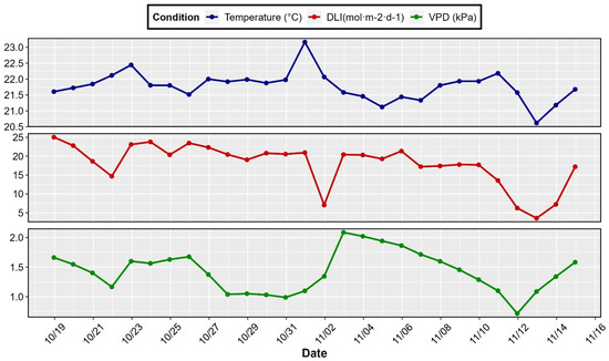
Figure 1.
Indoor environmental conditions (temperature, daily light integral [DLI], and vapor pressure deficit [VPD]) at the experimental greenhouse.
We addressed potential spatial heterogeneity in the greenhouse through several methodological choices. The experiment utilized localized environmental sensors positioned at the center of each tray to measure the DLI, allowing for tray-specific light condition data. Furthermore, treatments such as melatonin concentrations were randomized, and individual seedlings were randomly distributed across the trays to spread out any potential localized environmental effects. The use of an image analysis workflow to identify and extract data for each plant also helped to track and analyze morphological and spectral features on a per-plant basis, rather than relying on a single, overall average for the tray. Finally, for multispectral analysis, we deliberately focused on a central, delimited section of the images to ensure we were only using data from plants that received even illumination from the sensor’s lights.
A deep water culture hydroponics system was used to grow the plants. Six black trays with 243.8 × 121.9 × 20.3 cm (L × W × H) were distributed along a 15.24 m metallic bench inside the greenhouse. Each tray was filled with 200 L of fertilizer solution with a polystyrene foam insulation board (GreenGuard XPS; Kingspan Insulation, Atlanta, GA, USA) floating on top of the solution. Additionally, 55 holes with 2.54 cm diameter were drilled at 18 cm from hole center to hole center, at a density of 25 plants/m2 along the foam board, forming an 11 × 5 grid. Inside each hole, individual rockwool plugs with a single seedling were placed into a 4.45 cm top diameter × 3.18 cm bottom diameter × 4.76 cm deep net cup (Orimerc Garden, Seattle, WA, USA) as described in [20]. The fertilizer solution inside the trays was permanently aerated by four 5.08 cm air stones (Aquaneat, Madison, WI, USA) connected by 0.79 × 0.48 cm (outside × inside diameter) clear extruded acrylic tubes (Dernord; Tangxia, Dongguan, China) to 3.75 L/s at 0.048 MPa aeration pump with a 1.27 cm outlet (EcoAir 7; EcoPlus, Vancouver, WA, USA) to keep an ideal dissolved oxygen concentration for root development [20].
2.2. Plant Material, Growth Conditions, and Treatment Factors
Seeds of ‘Chicarita’ and ‘Dragoon’ romaine lettuce (both from Johnny’s Selected Seeds, Winslow, ME, USA) were germinated on 96-cell rockwool flats (AO 25/40 Plug; Grodan, Roermond, The Netherlands) placed on ebb-and-flow subirrigation benches located inside a vertical farm. Flats were subirrigated with a fertilizer solution prepared with a 15N-2.2P-12.5K water-soluble fertilizer (15-5-15 Cal-Mg Jack’s Professional LX; J. R. Peters, Allentown, PA, USA) with 100 mg L−1 nitrogen as described in [21].
After 12 days, the seedlings were transferred to a deep water culture system mounted inside a Venlo-type polycarbonate greenhouse. We used the same fertilizer solution recipe with 100 mg L−1 nitrogen, prepared using a 15N-2.2P-12.5K water-soluble fertilizer (15-5-15 Cal-Mg Jack’s Professional LX; J. R. Peters, Allentown, PA, USA). The fertilizer solution pH was maintained between 5 and 6, and the electrical conductivity from 1 to 2 mS cm−1. We subjected the plants to a multitude of conditions to have a wide range of visual symptoms to utilize our imaging system, using three melatonin concentrations (0, 5, and 10 µM), two lettuce cultivars (‘Chicarita’ and ‘Dragoon’), and two lighting regimens (natural sunlight and natural sunlight + supplemental light).
For melatonin, a control (no melatonin) and two different melatonin concentration levels (5 and 10 µM) were supplemented within each tray with fertilizer solution. Melatonin was used to induce a wider range of tipburn development patterns and symptom severities, thereby challenging the different imaging analytical approaches. For this, melatonin 99% powder (Xi’an Pincredit, Xi’an, China) was dissolved in water and added to a fertilizer solution to reach the final experimental concentrations. The idea was that higher melatonin rates would slow the onset of the tipburn symptom. Twenty-seven lettuce seedlings for each cultivar were randomly distributed among the 54 holes available in each growing tray. Cultivars were selected based on their predisposition to tipburn. ‘Dragoon’ was the most sensitive cultivar to tipburn, and ‘Chicarita’ is considered exceptionally tipburn-tolerant by the seed provider. The last treatment applied was supplemental lighting with two levels (presence or absence), with the additional lighting being added to rapidly increase plant growth and consequently induce tipburn symptoms. The growing bench was divided into two sections, where three trays within the first section had a light-emitting diode (LED) light fixture (Fluence SPYDRx, Fluence Bioengineering, Austin, TX, USA) overhead, while the other section did not have any supplemental lights. An extended photosynthetically active radiation (ePAR) quantum sensor (SQ-610 ePAR; Apogee Instruments, Logan, UT, USA) was positioned in the center of each tray’s insulation board measuring the photosynthetic photon flux density (PPFD). All sensors were connected to a datalogger (CR1000X; Campbell Scientific, Logan, UT, USA) and used to calculate the DLI attained for each tray with and without supplemental lighting over the crop cycle (Figure 2).

Figure 2.
Diagram representing the three experimental factors: supplemental lighting, melatonin concentration, and lettuce (Lactuca sativa) cultivars (‘Chicarita’ and ‘Dragoon’). Light treatments were fixed, while melatonin rates were randomized within each tray.
2.3. Morphometric Analysis Using RGB Image Processing
2.3.1. RGB Image Acquisition
For image capture, a Linux-based embedded microcomputer (Raspberry Pi 4 model B; Raspberry Pi Foundation, Cambridge, UK) and a 12-megapixel 120° Wide-Angle RGB camera (Raspberry Pi Camera Module v3; Raspberry Pi Foundation, Cambridge, UK) were used [21]. A script scheduler was implemented using the ‘crontab’ library to automatically run the scripts responsible for initiating the image capture process at three predefined times during the day, where first, second, and third captures were taken at 08:00, 12:00, and 17:00 h, respectively. The first two images were captured under natural sunlight, depending on the weather and cloud cover. The third capture occurred during a transitional period of natural light, in the presence of diminishing late-afternoon sunlight supplemented by artificial LED illumination. The camera module, operating in automatic mode, adjusted parameters such as exposure time, white balance, and International Organization for Standardization (ISO) sensitivity dynamically to accommodate the changing light conditions.
An embedded computer with its corresponding RGB camera was installed on top of each growing tray. The camera lens was positioned to point down towards the center of each tray, allowing top-view images to effectively capture all 54 plant canopies across the tray dimensions [21]. To ensure the camera field of view (FOV) effectively covered the tray completely, the camera working distance (WD), or the ideal height at which the camera was mounted to cover the whole tray and calculated using Equation (1). Here, the target horizontal and vertical FOVs correspond to the tray dimensions, while the angular FOV (AFOV) corresponds to the wide-angle RGB camera specification (120°) as described in [20].
For each embedded computer, RGB image capturing was implemented in Python using ‘Picamera2’ and ‘OpenCV’ ver. 4.8.1 [22]. Captured images were continuously stored within a cloud storage provider using the ‘rclone’ library to interface each embedded computer with the cloud storage platform. The rclone configuration was set up to link the embedded computer to a designated cloud storage platform account. An additional script was created to upload the captured images to the selected account using the same library described before.
2.3.2. Plant Detection and Instance Segmentation
To overcome the risk of canopy occlusion that complicates single canopy segmentation, Cardenas-Gallegos et al. [21] implemented an instance segmentation model to identify individual canopies and delimit them from the rest of the image. Briefly, the process began with data annotation, where 186 images were annotated using the Python library Anylabeling v0.3.3 [23], an Artificial Intelligence (AI)-assisted data labeling tool that uses the Segment Anything Model (SAM) from Meta AI to support the auto-labeling functionality [21]. The annotation quality was comparable to manually annotated masks, while the time allotted for image labeling was significantly reduced. A folder containing the image captures used for training was uploaded into the software’s interactive window. Here, the objects were automatically segmented by selecting a pixel that belonged to an object, and incorrectly segmented points could be excluded to refine the object contour limits. At the end of this process, a label name was entered before saving the object, and each object label name with the corresponding coordinates within an image was stored as a .JSON file [21].
A custom YOLOv8 model [24] was implemented using a software (Python version 3.11.5; Python Software Foundation, Wilmington, DE, USA) with ‘PyTorch’ [25] and ‘Ultralytics’ libraries [20]. Weights from a pre-trained segmentation model trained with the Common Objects in Context (COCO) dataset were used as transfer weights for the new custom model. A .YAML file was created, which contained the name and count of the classes (only plant class in this context) available in the annotated data and locations of folder directories for train, validation, and test sets. The custom model was trained with 186 images with a resolution of 1920 × 960 pixels, the number of epochs was set to 100 with a patience of 0 (early stopping disabled to avoid issues) and with a batch size set to 4, a value that specifies the number of images taken from the training set to estimate the error gradient. The model’s performance was evaluated using 30 randomly selected unseen images.
Given the intensive computing power required to train an object detection model, training was performed using the Google Colaboratory ecosystem. This cloud computing service offers access to on-demand graphics processing unit (GPU) hardware acceleration, along with a built-in platform featuring Python, TensorFlow, and Jupyter Notebooks [21]. The A100 graphics processing unit, equipped with 40 GB of RAM (A100 SXM4-40GB; NVIDIA, Santa Clara, CA, USA), was selected as the hardware accelerator by choosing it as the runtime type in the drop-down menu available for each notebook within the platform [21]. Figure 3 depicts the single canopy detection achieved by the YOLOv8 model results for captures performed for different canopy sizes.
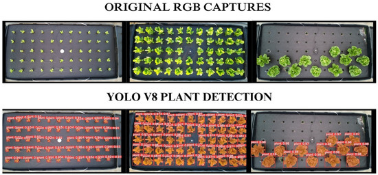
Figure 3.
Instance segmentation implemented using a custom YOLOv8 Segment model. The top image displays the original red, green, and blue (RGB) captures for three different stages of the lettuce (Lactuca sativa) crop, and the bottom image shows the results after using the model to predict the location of individual plant objects within the original RGB captures.
2.3.3. Morphometric Plant Features Extraction
A script was implemented using the libraries ‘OpenCV’ and ‘Scikit-Image’ for image processing, while ‘Ultralytics’ was used to implement a YOLOv8 pre-trained model to perform instance segmentation for plant identification. Briefly, our workflow was organized as follows: (1) Input raw RGB images with 1920 × 960 pixels. (2) Load pre-trained weights from the previously trained plant detection YOLOv8 model. (3) Use the object detection model to identify individual plants within the image dimensions and use the identified bounding boxes to extract the canopy mask and centroids. (4) The x- and y-axis centroid positions for each extracted mask were used as a reference to define an iteration order and assigned a unique identification number that ensures that the mask iteration loop on the next step followed the same order for each image during the plant identification step. (5) Another loop iterated across the extracted lettuce canopy masks to obtain all morphometric properties, associating each feature with the plant identification number. (6) Finally, a dataset containing nine features describing the canopy’s geometry for each plant was created and stored as a .csv file for data processing. YOLOv8 segmentation accuracy output both bounding box (B) and mask/segmentation (M) metrics (Table 1).

Table 1.
YOLOv8 segmentation accuracy bounding box (B) and mask/segmentation (M) metrics.
As an additional feature, the canopy area obtained per plant and the DLI calculations per growing tray were used to estimate a daily incident light value, the amount of light each lettuce head accumulated between two time points [26]. The plant canopy area (in pixels) was transformed into canopy area (cm2) using a conversion factor based on the known length (cm) of a reference object within the image and divided by the length in pixels of the same reference object. Then, the cumulative DLI on a specific day obtained from the sensor in mol m−2 d−1 was multiplied by the area in cm2 to obtain a unique incident light value per plant in moles. This calculation assumes that all plants within a tray received the same light intensity across the insulation board. All extracted features for each plant are summarized in Table 2.
Table 2.
Geometrical features were extracted using an image processing workflow from RGB color captures. Features describing canopy shapes were extracted per plant and used as potential predictors for the regression models, similarly to [20].
2.4. Biomass Estimation Modeling
2.4.1. Plant Biomass Measurements
To obtain ground-truth measurements for image-based plant growth and morphometric features, conventional destructive sampling of aboveground biomass from 324 plants was used to quantify leaf fresh weight, leaf and root dry weight, and leaf area. We used 168 plants for harvest #1, 78 plants for harvest #2, and 78 plants for harvest #3. For leaf and root dry weight, plant shoots and roots were dried in a drying oven at 80 °C for 72 h. Leaf area was measured with a leaf area meter (LI-3100; LI-COR, Lincoln, NE, USA) for every leaf on each harvested plant [20]. In total, three harvests were performed along a 26-day lettuce crop cycle. The first, second, and third harvest rounds were performed at 12, 19, and 26 days after transplant (DAT), respectively. All plant observations from the three harvest rounds were combined in a single dataset. In this dataset, each observation represented a single plant with measured leaf fresh weight, leaf and root dry weight, and leaf area values organized in columns [20]. Additionally, one column specified the harvest date for each plant.
For the last two harvest rounds, tipburn development was evaluated based on the percentage of leaves from the total leaf count showing tipburn symptoms and the tipburn incidence corresponding to the plant count within a particular treatment that developed tipburn symptoms. Tipburn is a plant physiological disorder caused by localized calcium deficiency in rapidly growing leaf tissues. It manifests as necrotic lesions or browning at the leaf margins, often due to inadequate calcium transport rather than a lack of calcium in the growing medium. Factors such as high humidity, excessive nitrogen fertilization, and rapid growth under high light or temperature conditions can exacerbate tipburn. Tipburn incidence refers to the frequency or proportion of plants affected by tipburn within a given population or production system, serving as an indicator of crop susceptibility and overall growing conditions.
2.4.2. Model Training
Model training, hyperparameter optimization, and performance evaluation were conducted using R [27], RStudio 2024 version 4.4 [28] and the tidymodels package [29]. Models were fit for each response variable (leaf fresh weight, leaf and root dry weight, and leaf area) following a supervised learning strategy [30]. Here, response variables collected destructively were used as the expected response values or labels as described in [20]. Canopy shape features extracted with the image processing step outlined in Section 2.3.3 were used as potential predictors and/or independent variables. The canopy area was not included in the features list to avoid redundancy, as incident light already integrates canopy area into its estimate. Additionally, the cultivar name ‘Chicarita’ or ‘Dragoon’ was considered a categorical variable and added as an additional predictor.
The final dataset used to build each model consisted of 324 observations, where 168 plants came from the first harvest round (12 DAT), 78 came from the second (19 DAT), and 78 plants came from the last harvest round (26 DAT) [20]. Additionally, 10 morphometric variables distributed across the matrix columns were used as potential predictors for each observation organized in rows. The total number of observations from the original data matrix was split into two sets, where 70% (n = 225) of all observations were used for model training and 30% (n = 99) of all observations for model validation on unseen data [20].
2.4.3. Modeling Techniques
To improve the prediction accuracy for each biomass parameter using a multiple trait canopy description, models with increasing levels of complexity were fitted and compared [20]. For the baseline model, two alternatives were assessed: a simple linear regression and a logarithmic regression. Both models fit using the image feature that showed the greatest coefficient of determination (R2) after fitting a simple regression model for a particular response with each feature available.
Two machine learning approaches were also implemented, including LASSO and random forest regression. As most of the geometric image-derived predictors were calculated from the same canopy shape, there was a high risk of correlations among them. For this reason, algorithms less sensitive to multicollinearity were selected [20]. LASSO regression represents a regularized linear model that optimizes performance by evaluating the contribution of each feature to the final model by including or excluding variables based on model performance under a range of different penalty value (λ) scenarios. Lambda is used as a threshold criterion to limit the parameter increase to only those features that contribute significantly to the reduction in the sum of squares error (SSE). As LASSO penalizes absolute values instead of a second-order penalty (L2), coefficients can be set to absolute zero, serving as a regularization and an internal feature selection step. If the penalty is large, LASSO favors a simpler model where many feature coefficients are reduced to zero [20]. Conversely, a small penalty value yields a more complex LASSO model with more features [31]. Before training, a preprocessing step was implemented to normalize (feature relativization) all potential predictors to numbers from 0 to 1 to ensure variables are not over or underweighted due solely to differences in orders of magnitude [20]. The optimal L1 regularization parameter λ was then chosen, as it determines the strength of the penalty on the coefficients. Parameter optimization was performed using an iterative search procedure using the tune_sim_anneal function from the tune package [32] in R using a five-fold cross-validation resampling technique. The value of lambda that outputs the model with the lowest root mean squared error (RMSE) and highest determination coefficient (R2) was selected as the hyperparameter value to fit the final model.
According to Cardenas-Gallegos et al. [20], random forest regression is an ensemble machine learning method based on decision trees that combine multiple predictions to improve overall performance and reduce overfitting. In addition to the random subsets of data used to train individual trees (bootstrap aggregation), it reduces the variance of the predictions even further by adding another random component when selecting predictors to build each tree [20,33]. This algorithm is preferred among others because of its high accuracy but is even more significant for its flexibility when dealing with outliers, missing data, and features with different scales. Moreover, fewer preprocessing steps are required with a random forest [20,29].
For hyperparameter tuning, a pre-defined set of tuning parameters was organized in a grid to explore a range of possible values for the most influential random forest model, including; (1) mtry, number of predictors to be considered for each new split, ranging from one to the number of predictors present in the matrix; and (2) min_n, is the minimal node size or the number of observations needed to keep splitting nodes. To select the model with the best hyperparameter combination, a five-fold cross-validation resampling technique was implemented using only the training set, while the test set was held out for performance validation. The parameter combination that outputs the model with the lowest RMSE and highest R2 was selected to apply its hyperparameter value to fit a final random forest model.
2.5. Prediction Performance Metrics
All the model’s predictions were compared with the biomass parameters measured destructively. Three performance metrics calculated using the observations from the dataset were used to describe precision and accuracy across models. The metrics included.
- (1)
- R2, which indicates the proportion of variance in the response (dependent variable) that is explained by the predictors (independent variables) used in the model [20]. This metric represents a useful consistency reference but not the accuracy [31].
- (2)
- RMSE, which computes the square root of the difference between actual and predicted values. As the error values are squared, RMSE is useful to detect larger errors. Additionally, the interpretation is more straightforward since the square roots transform the value to the same units as the response [20].
- (3)
- Symmetric Mean Absolute Percentage Error (SMAPE): Unlike the previous metrics, SMAPE is independent of the square function. Instead, it uses the absolute differences between the actual and predicted values, treating all errors equally regardless of their direction. It expresses the average absolute error as a percentage to better understand the relative size of errors [20]. The symmetry that characterizes this metric considers both underestimation and overestimation and provides a more balanced metric of error measurement when small and large values are present.
2.6. Multispectral Image Analysis
The research used multispectral imaging to detect early signs of tipburn susceptibility in lettuce. Researchers selected specific wavelengths and vegetation indices for analysis because they are known to reflect physiological changes in plants. The photochemical reflectance index (PRI) is an indicator of photosynthetic efficiency, and the red-edge chlorophyll index (CIrededge) indicates more efficient photosynthesis and a faster growth rate that likely contributed to its susceptibility.
2.6.1. Image Acquisition
Multispectral images were captured by an alpha version of the RAYN Vision System (RAYN Growing Systems, Middleton, WI, USA). This multispectral sensor integrates nine monochromatic LED lights and a white LED light with specific mean peak wavelengths ranging from 475 to 940 nm (Table 3), with manual calibration workflows and required specific adjustments for light uniformity. To isolate the spectral information associated with each wavelength, the sensor uses a monochromatic camera with a 120° lens that captures images with a resolution of 1280 × 800 pixels, where each pixel value corresponds to the pixel intensity of each band as each LED light turns on and off one at a time. After capturing all monochromatic images, the sensor combines all spectral bands into a multispectral image cube, storing the pixel intensity information for each wavelength. To yield comparable results among sensors, capture settings configuration, including exposure time, sensitivity, and LED light brightness, was identically set up for all six sensors using each camera web interface. Additionally, the sensor mounting height above each growing tray was fixed at the same vertical distance from the insulation board on top of the deep water culture hydroponics trays to the camera lens. Sensor positions were maintained across the crop cycle to ensure consistency for all captures. Since spectral reflectance information gathered depends on the distribution of LEDs as an external light source, the manufacturer recommended a theoretical imaging area to guarantee a surface area where light is evenly distributed within the camera at a particular mounting height (~1 m). To avoid the excessive reflectivity produced by the insulation board from a top-view perspective, a non-reflective black fabric was used to cover the insulation board on each growing tray as described in [21].
Table 3.
Wavelength components for each light-emitting diode (LED) light source used as an active illumination source by the multispectral sensor. Where NIR = near-infrared.
The multispectral images generated with the sensor can be pre-processed and analyzed with the open-source analysis software RAYN Vision System Analytics [34] (https://github.com/rayngrowingsystems/RVS_Analytics) (accessed on 26 September 2025). These images were normalized to reduce noise caused by ambient stray light using a dark reference, recorded as part of the imaging process.
2.6.2. Multispectral Image Processing Workflow
Image captures were programmed using the camera web interface scheduler functionality and stored internally in each camera’s external storage with a specific identification number and the timestamp corresponding to each capture. All captures were taken at night, in complete darkness, to ensure that the only light source hitting plant canopies was the active illumination LED source. After capturing one monochromatic image per LED light, an .ENVI file containing 10 arrays of pixel size 1280 × 800 stored pixel intensity information for all nine bands plus an additional dark reference band that corresponded to a monochromatic image captured in complete darkness without any active LED light source. A header (.HDR) file containing metadata that described the acquisition time, pixel resolution, data format, and the number of available bands was recorded.
For processing, pixel intensity values for all wavelengths were retrieved from the .ENVI file generated. The pixel values of the dark reference band were subtracted from the pixel intensities of the nine available bands to account for any potential background noise coming from the surrounding environment. These calibrated pixel intensity values were normalized to obtain reflectance values between 0 and 1. For plant pixel segmentation, the band that provided the better contrast between plant canopies and the background was selected to generate a binary mask based on a pixel intensity threshold value. The binary mask was delimited to a rectangular section in the center of the image, rejecting plant canopies with an uneven distribution of LED lights outside the theoretical surface imaging area. Within this delimited area, eight plant canopies were isolated by cropping a rectangular section of the full-size image (Figure 4). A grid-based location system using x and y coordinates grouped pixels belonging to the same plant, identifying individual canopies as distinct objects. Each canopy was assigned a unique plant identification number through a labeling system, organizing regions of interest in a defined order. This identification system was used to track individual plant reflectance outputs across time. The reflectance values for each plant were obtained by overlapping the binary mask on top of the calibrated spectral data retrieved. The mask was applied to each of the nine-pixel arrays, with a pixel size of 1280 × 800, to obtain only the reflectance corresponding to the plant canopy for each waveband. The output of the analytical workflow was a dataset containing mean, maximum, and minimum reflectance values per plant.

Figure 4.
A multispectral image analytical workflow was used to extract reflection intensities from all images captured under a specific LED light radiation. The imaging area and plants considered were reduced to avoid values from plants with uneven light distribution.
2.6.3. Vegetation Indices Calculation
Based on the same multispectral analytical workflow, nine vegetation indices (VIs) were calculated using the closest specific sensor’s band wavelengths available as an alternative to the theoretical wavelengths due to commercial availability (Table 4). Reflectance values for the nine bands captured by the MultiSpectral Instrument (MSI) sensor were used as input for vegetation index calculation functions available in the Python library PlantCV ver. 4.0.1 [35], which automatically selected the required bands for a specific index from reflectance values. If the exact wavelength needed for calculation were missing from the spectral array object, the function would select the next closest band (the maximum distance is considered added as an argument).
Table 4.
List of vegetation indices calculated using reflectance intensities per plant.
2.7. Statistical Analysis
The experiment was designed to generate a broad gradient of tipburn severity in lettuce to develop and validate an imaging-based model. To achieve this, plants were treated with various melatonin concentrations to intentionally induce a range of symptom expressions. Given that the study’s primary objective was to supply the imaging model with varied data rather than to formally test melatonin’s effects, our analysis focused on descriptive statistics. We present means and 95% confidence intervals to summarize the relationship between melatonin concentration and tipburn severity, thereby documenting the successful creation of a symptom gradient suitable for our modeling purposes. Due to spatial limitations related to the imaging sensors’ fixed positions across the growing bench and the size of the trays used, increasing the number of replicates was not feasible, precluding a sufficiently replicated, blocked ANOVA or comparable GLMM full model, since there was not enough statistical power to conduct a formal analysis. Our approach was necessarily conservative, given the need to maintain a sufficient number of plants to enable destructive sampling in conjunction with the chronosequence of imaging objectives (the main focus of this study).
3. Results
3.1. Effect of Melatonin on Biomass Accumulation
The effect of melatonin on leaf fresh and dry and root dry biomass was evaluated at the end of the growing cycle, 26 DAT (Figure 5). Error bars representing 95% confidence intervals suggested that melatonin had no detectable effect on biomass in any of the cultivars, regardless of the presence or absence of supplemental lighting.
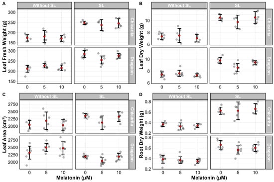
Figure 5.
Effects of three melatonin concentrations (0, 5, and 10 µM) on two lettuce (Lactuca sativa) cultivars (‘Chicarita’ and ‘Dragoon’) grown with (supplemental lighting SL) or without supplemental lighting (Without SL) on leaf fresh weight (A), leaf dry weight (B), leaf area (C) and root dry weight (D). Red dots represent the mean (n = 7 plants) ± 95% confidence intervals.
3.2. Cultivar and Supplemental Lighting Effects on Biomass
Differences in leaf fresh biomass were observed between cultivars growing without supplemental lighting, with ‘Dragoon’ accumulating 25% greater leaf fresh weight than ‘Chicarita’. Under supplemental light, the trend was similar but less obvious, with ‘Dragoon’ showing 10% greater leaf fresh weight accumulation compared with ‘Chicarita’. The effect of light treatment on fresh weight biomass appeared to be cultivar-dependent. ‘Chicarita’ exhibited a 39% increase in leaf fresh weight under supplemental light compared to its growth without supplemental light, whereas ‘Dragoon’ showed a more modest increase of 24% in fresh weight under the same conditions (Figure 6A).

Figure 6.
Mean (± 95% confidence intervals) of leaf fresh weight (A), leaf dry weight (B), leaf area (C) and root dry weight (D) for lettuce (Lactuca sativa) plants (n = 7) ‘Chicarita’ and ‘Dragoon’ grown with supplemental light (SL) or without supplemental light (Without SL).
A comparison of leaf dry weights among cultivars revealed no differences in dry biomass accumulation without supplemental lighting. However, under supplemental light, ‘Chicarita’ produced 11% more dry biomass than ‘Dragoon’. ‘Chicarita’ accumulated 41% more dry weight under supplemental light than its growth without additional light, while ‘Dragoon’ exhibited a smaller increase of 24% in dry biomass under supplemental light relative to its growth without supplemental light (Figure 6B).
The effects of both cultivar and light conditions on leaf area were also evaluated. Without supplemental light, ‘Dragoon’ exhibited 16% greater leaf area than ‘Chicarita’ under the same conditions. However, supplemental light reversed this trend, with ‘Chicarita’ showing 6% greater leaf area than ‘Dragoon’. Assessing the impact of light on leaf area within each cultivar, ‘Chicarita’ grown under supplemental light displayed a 9% increase in leaf area compared to its growth without additional light, while ‘Dragoon’ experienced a 14% reduction in leaf area under supplemental light compared to plants grown without it (Figure 6C).
Root dry weight showed the most pronounced differences between light treatments, with plants grown under supplemental light accumulating approximately 50% more root biomass than those grown without it, regardless of cultivar. However, no differences or clear trends emerged when comparing root dry weight between cultivars under the same light conditions (Figure 6D).
Tipburn Development Evaluation
Subtle tipburn symptoms were first observed between 12 and 13 DAT. For this reason, tipburn was quantified only for harvests two and three. For both harvest periods, only plants grown under supplemental lighting treatments exhibited visible tipburn lesions. A fertilizer solution concentration analysis was carried out for all growing trays at the end of the crop cycle (Table 5). The calcium concentration was approximately the same in all trays, and it was not a limiting factor that triggered tipburn development. Trays growing under supplemental lighting (T01, T02, T03) exhibited tipburn, despite having a similar calcium concentration to trays without supplemental lighting (T04, T05, T06). Higher DLI values across the crop cycle for the trays with supplemental light, measured using a localized quantum sensor on top of each growing tray, confirmed a more pronounced effect of the light treatment on the development of the disorder rather than a nutritional disturbance (Figure 7).
Table 5.
Detailed fertilizer solution concentrations per growing tray (treatment) at the end of the crop cycle. T1–T6 represents the tray identification number associated with each combination of treatment factors.

Figure 7.
Daily Light Integral (DLI) variation across growing trays throughout the crop cycle. Trays identified by a tray ID from T01–T06. Colors differentiate trays cultivated under supplemental lighting conditions (red) and those grown without supplemental lighting (blue). Values were calculated based on precise photosynthetically active radiation (PAR) sensor readings.
Tipburn incidence and severity were used to quantify the development of the disorder at 19 DAT and at the end of the crop cycle (26 DAT) (Figure 8). A similar response was observed for ‘Chicarita’ and ‘Dragoon’ grown under 5 µM melatonin, where both incidence and severity were lower concerning the control and a higher melatonin concentration. Nevertheless, this pattern is inconsistent for the second harvest date, where 5 µM had a similar incidence and severity as the control and 10 µM melatonin. The difference in tipburn development was more evident among cultivars, where ‘Dragoon’ showed a higher tipburn incidence and severity for both harvest dates than cultivar ‘Chicarita’.

Figure 8.
Tipburn evaluation for different lettuce (Lactuca sativa) cultivars (‘Chicarita’ and ‘Dragoon’), grown under three melatonin concentrations (0, 5, and 10 µM) under supplemental lighting on a second harvest round 19 days after transplant (DAT) and third harvest round (26 DAT). (A) Tipburn incidence and (B) Tipburn severity calculated as the percentage of infected leaves. Bars and red dots represent the average ± 95% confidence intervals of 7 plants (n = 7).
3.3. Morphometric Analysis Using RGB Image Processing
The canopy area did not show any statistically significant differences between the three melatonin treatment concentrations. For both cultivars grown without supplemental lighting, 5 µM melatonin may have resulted in a quicker increase in canopy area compared to 0 and 10 µM melatonin. However, treatments were not statistically significant based on the 95% CI overlap. No apparent trend based on melatonin concentrations was observed for any of the cultivars grown under supplemental lighting (Figure 9).

Figure 9.
Canopy area in pixels across time comparing the effect of three melatonin concentrations (0, 5, 10) for two different lettuce (Lactuca sativa) cultivars (‘Chicarita’ and ‘Dragoon’), grown with or without supplemental lighting. Means obtained from 26 or 28 individual lettuce plants. Black dots represent the average ± 95% confidence intervals of available plants on a given day.
Canopy area began to diverge at 18 DAT, where cultivar ‘Chicarita’ had a steeper increase than ‘Dragoon’ (Figure 10). Conversely, ‘compactness’ and ‘extent’ were the features that displayed the most contrasting pattern associated with cultivar and supplemental light. Without supplemental light, ‘Dragoon’ values for compactness and extent were noticeably greater than the measurements from ‘Chicarita’. In the presence of supplemental light, there appeared to be only minor differences, when present, between ‘Dragoon’ and ‘Chicarita’ as DAT increased (Figure 10).

Figure 10.
Lettuce (Lactuca sativa) canopy morphometric features across time for two cultivars (‘Chicarita’ and ‘Dragoon’) grown with or without supplemental lighting. Each point represents the mean feature value of 78 or 84 plants for ‘Chicarita’ and ‘Dragoon’, respectively. Black dots represent the average ± 95% confidence intervals of available plants on a given day.
3.4. Biomass Estimation Modeling
A correlation matrix was used to index multicollinearity among all morphometric features extracted from image processing and incident light. Pearson’s coefficients reveal a high level of correlation among six out of 10 predictors, with correlation values exceeding 0.90, indicating a significant risk of multicollinearity. The canopy area in cm2 and diameter showed the highest correlation coefficient, while plant perimeter and eccentricity had the lowest coefficient (Figure 11). Although incident light was calculated from the canopy area (cm2) it did not show correlation coefficient values as high as those between canopy area and other predictors (Figure 11).
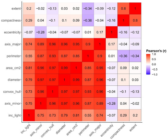
Figure 11.
Correlation matrix showing Pearson’s correlation coefficient values between canopy geometrical features used as potential predictors obtained using image processing. The red color indicates a high positive correlation coefficient between a pair of variables, while the purple color shows a high negative correlation coefficient.
Plant diameter, incident light, and canopy area (cm2) were the predictors showing the greatest R2 from a series of simple linear regression models. Incident light was selected as the best potential predictor for leaf fresh weight, as it combined canopy and light exposure (Figure 12).

Figure 12.
Coefficient of determination (R2) for five morphometric features with the greatest values obtained after fitting a simple linear regression model between each response variable and each morphometric feature extracted from the image processing workflow. The features with the highest values were used as predictors for the linear model for baseline prediction.
Before the training process, a hyperparameter tuning step was implemented using a resampling technique based on observations from the training set. The range of values used to optimize performance for both machine learning prediction models to predict leaf fresh weight is summarized in Figure 13. For LASSO regression, a lambda (λ) L1 regularization value of 0.02 yielded the model with the lowest RMSE, while for Random Forest mtry and min_n values of 6 and 5, respectively, resulted in the best hyperparameters combination for the optimum model when compared among those with the lowest RMSE. The tuned model was trained using all observations available in the training set before running predictions on the unseen test dataset.

Figure 13.
Hyperparameter tuning for leaf fresh weight prediction using five-fold cross-validation resampling technique for two machine learning models parameters: (A) Effect of LASSO regression lambda regularization value on root mean square on top and R2 in the bottom graph, (B) effect of Random Forest mtry and min_n values. The vertical dashed lines show the best parameter selected based on the lowest root mean squared error (RMSE).
To measure the tuned models’ predictive utility, estimates obtained from a test set were used to calculate three performance metrics (R2, RMSE, and sMAPE). For comparison, the predictive ability of the baseline model was included to represent the gain in performance with additional complexity.
For leaf fresh weight, the random forest model outperformed less complex models, yielding the most accurate predictions, as indicated by its reduction in RMSE and sMAPE. Compared with LASSO regression, the random forest model decreased the percentage error from ~34% to ~13%, corresponding to growth parameter units of 34.14 and 17.32 g, respectively. The random forest model explained the greatest proportion of variation compared to other competing analyses (Figure 14).

Figure 14.
Scatterplots for measured and estimated leaf fresh weight on unseen observations from a test set. Estimation results from (A) a simple linear regression model fitted using incident light as a predictor, (B) a logistic regression model fitted using incident light as a predictor, (C) a LASSO regression model fitted based on the predictors selected by the model’s optimized penalty and (D) a random forest regression model using all potential predictors.
Likewise, more complex modeling strategies improved predictive performance for leaf dry weight estimations. The random forest model outperformed LASSO regression, as indicated by a reduction in the percentage error from ~20% to ~12%, corresponding to growth parameter units of 0.87 and 0.72 g, respectively. Random forest represented the greatest variation in the leaf dry weight data (~94%) compared with the other competing analyses (Figure 15).

Figure 15.
Scatterplots for measured and estimated leaf dry weight on unseen observations from a test set. Estimation results from (A) a simple linear regression model fitted using incident light as a predictor, (B) a logistic regression model fitted using incident light as a predictor, (C) a LASSO regression model fitted based on the predictors selected by the model’s optimized penalty and (D) a random forest regression model using all potential predictors.
The random forest model performed the best, providing the most accurate estimations with a percentage error of 10.9%. This represented a ~9% improvement over the LASSO model and a ~19% improvement over the linear regression model. The LASSO model ranked second, achieving an R2 of 0.91 and reducing the estimation error by about 10%. In contrast, both the linear and logistic regression models performed poorly, with metrics similar to those of the linear model and no significant improvement in the leaf area model’s performance (Figure 16).

Figure 16.
Scatterplots for measured and estimated leaf area on unseen observations from a test set. Estimation results from (A) a simple linear regression model fitted using incident light as a predictor, (B) a logistic regression model fitted using incident light as a predictor, (C) a LASSO regression model fitted based on the predictors selected by the model’s optimized penalty and (D) a random forest regression model using all potential predictors.
3.5. Multispectral Image Analysis
MSI captures were performed between 5 and 12 DAT. For calculations, plant observations considered for both reflectance and vegetative index information were limited to eight plants to ensure that LED supplemental light was evenly distributed over the plants being imaged. Because there was no compelling evidence that melatonin had an impact on leaf tipburn, plant observations were pooled by cultivar and supplemental light treatment factors to assess multispectral imaging on tipburn development (Figure 17). Based on mean reflectance values per band for each cultivar, ‘Chicarita’ showed higher mean reflection for bands between 500 and 665 nm for plants grown under supplemental light (Figure 14 and Figure 15). Conversely, mean reflectance values for three bands measured above 665 nm were greater for ‘Dragoon’, even though the overlapping confidence intervals did not strongly suggest a significant difference between these cultivars (Figure 15). For wavelengths above 665 nm, the MSI sensor captured information for one wavelength within the red edge (740 nm) and two wavelengths within the near-infrared (NIR) (850 nm and 940 nm). Spectral signatures under supplemental light showed a similar pattern for both cultivars, with subtle differences in 850 nm and 630–665 nm, where mean reflectance values were lower than those obtained without supplemental lighting (Figure 18). Although a similar pattern was shown, the difference in the mean reflection above 665 nm was more evident when comparing cultivars under supplemental light.

Figure 17.
Spectral signature comparison between cultivars grown under supplemental lighting (SL) or without supplemental lighting (Without SL) obtained after measuring reflectance from nine spectral bands. Each observation (dot) represents the mean reflectance in each wavelength for 12 plants.
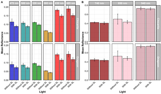
Figure 18.
Mean reflectance comparison between cultivars grown under different light conditions for all available 400–950 nm bands. (A) Available bands within the visible light spectrum (475, 500, 526, 595, 630, and 665 nm). (B) Available bands within far-red (740 nm) and near-infrared spectrum (850, 940 nm). Error bars represent upper and lower confidence intervals at 95%.
Since our strategy involved an anticipation monitoring system to alert to the potential development of tipburn, based on plant properties (as opposed to fertilizer solution levels), multispectral captures were carried out eight days before the first anticipated visual symptoms appeared. None of the indices showed evidence suggesting different trends between cultivars grown without supplemental lighting on the last day before visual symptoms appeared (Figure 16). Conversely, plants grown under supplemental light showed mean index values for CIrededge, enhanced vegetation index (EVI), normalized difference vegetation index (NDVI), and PRI were 56%, 13%, 27% and 13% higher for ‘Dragoon’ (more prone to tipburn) compared to ‘Chicarita’ plants grown under the same conditions, respectively (Figure 19).

Figure 19.
Changes over time for four vegetation indices (CIrededge, enhanced vegetation index [EVI], normalized difference vegetation index [NDVI], and photochemical reflectance index [PRI]). The graph highlights differences between two lettuce (Lactuca sativa) cultivars (‘Chicarita’ and ‘Dragoon’), grown with or without supplemental lighting.
Comparison of temporal changes in indices revealed different trends between plants of the same cultivar grown with and without supplemental light (Figure 20). The PRI exhibited a clear difference between the two light conditions. For ‘Dragoon’, plants grown under supplemental light had an 18% higher mean PRI value than those without supplemental light across all observation days. The difference for ‘Chicarita’ was even more pronounced, with a 76% higher mean PRI value under supplemental light observed on the last day before the first signs of tipburn appeared.

Figure 20.
Changes over time for four vegetation indices (CIrededge, enhanced vegetation index [EVI], normalized difference vegetation index [NDVI], and photochemical reflectance index [PRI]). The graph highlights differences between plants grown with or without supplemental lighting within a particular lettuce (Lactuca sativa) cultivar (‘Chicarita’ and ‘Dragoon’).
4. Discussion
4.1. Melatonin Effects on Growth and Tipburn Development
Controlled environment agriculture (CEA) systems enhance resource utilization to sustain continuous and accelerated growth rates, yielding multiple crop cycles within a reduced timeframe. Lettuce productivity has been limited by the susceptibility of many cultivars to tipburn, as cultivars were not bred to thrive under the intense conditions of CEA. Current tipburn avoidance strategies are oriented towards environmental modifications. In this study, melatonin was evaluated as an external amendment to the fertilizer solution in hydroponic systems to assess its potential in preventing tipburn without altering any environmental factors that could impact lettuce productivity. The melatonin concentrations applied in this experiment were limited and suggested that there were unlikely to be large differences in plant shoot or root growth. Conversely, in a preliminary study, melatonin concentrations were tested at 60 and 600 µM, and these higher concentrations had a detrimental effect on growth, particularly at the highest concentration, rather than promoting growth.
However, melatonin was not an effective strategy for alleviating tipburn at the concentrations set in this study, which aimed to induce a range of different symptoms for imaging detection. In a study assessing the mechanisms governing tipburn development, Carassay et al. [36] demonstrated the contribution of oxidative stress (particularly O2− production) to tipburn symptom development. Specifically, lettuce varieties resistant to tipburn exhibited higher antioxidant enzyme activity, which mitigated oxidative stress and prevented symptom development. A widely discussed mechanism governing the stress-alleviation potential of melatonin is the enhancement of the antioxidant machinery, which boosts the activity of antioxidant enzymes that scavenge reactive oxygen species (ROS) (Kumari et al., 2023) [10]. This suggests that a mechanism that improves antioxidant capacity could counter tipburn syndrome.
Tipburn is often associated with environmental conditions that restrict evapotranspiration and limit bulk water flow, resulting in limited calcium mobility in younger leaves. Biradar and Meng [8] evaluated the feasibility of using an exogenous calcium-mobilizing biostimulant inside the fertilizer solution of a lettuce crop growth hydroponically to mitigate tipburn. The highest concentration of the biostimulant (220 μL⋅L−1) showed an 88% and 85% reduction in the tipburn rating and the number of leaves with tipburn, respectively. Alternatively, instead of a mobilizing agent, improving physiological traits related to conductivity could help reduce the effects of restrictive mass flow. Exogenous melatonin application has significantly impacted gas exchange traits, such as stomatal conductance and transpiration, showing potential to improve restricted mass flow and, hence, symptom development [37].
4.2. Multispectral and Morphometric Signals Associated with Tipburn Development
Lettuce growth dynamics comparison using image analysis was implemented as a monitoring tool to characterize tipburn development for two lettuce cultivars. In this study, nine morphometric features used to characterize changes in canopy shape over time were described to describe the growth dynamics of two lettuces. The results showed that additional shape properties displayed useful morphometric changes over time, differentiating growth between two romaine lettuce cultivars with varying susceptibility to tipburn.
Extent and compactness were selected as most influential because of their contrasting trend as opposed to more common shape features, such as area or perimeter, which did not show any contrast between cultivar or supplemental lighting. Technically, compactness was obtained using the object area divided by the convex hull area of the same object, suggesting plants with higher compactness have leaves closely packed together, while lower values of extent and compactness indicate a less compact, more sparse leaf arrangement. Both cultivars under supplemental lighting showed more compactness and greater extent values, possibly explaining the higher incidence of tipburn under supplemental lighting. A closed, more compact canopy would create a barrier that inhibits an efficient transpiration rate, thereby establishing ideal conditions for the development of tipburn symptoms.
Using image-derived features extracted from lettuce canopies, Story et al. [17] implemented a machine vision monitoring system to anticipate tipburn in plants with induced calcium deficiency. Here, the projected canopy area was one of the features used to identify the onset of stress, besides three textural features, demonstrating the potential of a temporal evaluation of the canopy area to anticipate severe calcium deficiency. In our study, the projected canopy area did not show a particular pattern between plants grown under supplemental lighting and plants without it, most likely due to a different trigger of the tipburn development, that in this case, was not a depletion of calcium but an increase in overall light levels for the plants that showed higher tipburn symptoms due to the more vigorous growth that leads to the relative deficiency of calcium [2,7].
4.2.1. Biomass Estimation
An optimal combination of image features, integrating plant structural information and environmental sensors, can significantly enhance biomass estimation by capturing the environmental factors that affect plant growth throughout its cycle. Golzarian et al. [38] demonstrated that a simple linear regression model using plant area and dry weight, derived from top and side view images, outperformed other non-linear models. However, adding plant age as a predictor alongside plant area further improved prediction accuracy. In our experiment, we found that combining canopy size and available light into a single variable outperformed a simple linear regression model based solely on plant canopy area for predicting fresh and dry weight. Furthermore, machine learning models, such as random forest, were implemented to assess the potential of integrating multiple features to better represent biological responses. The random forest outperformed a LASSO regression model, likely due to its resistance to multicollinearity, as evident in the results, where many variables exhibited high collinearity [39].
4.2.2. Multispectral Image Analysis
In our study, we captured reflectance information and implemented two approaches to analyze multispectral data per plant. The first approach considered a mean reflectance analysis for each band on the last day of multispectral image capture (12 days after transfer), a day before the first visible symptom appeared. Analyzing reflectance per band could suggest an early stress situation where plants’ reflectance pattern showing a stress condition is characterized by an increase in visible (VIS) region reflectance, caused by a decrease in chlorophyll content and hence an increase in reflection in this region, together with a reduction in NIR reflectance that describes changes in internal leaf structure [40].
Physiologically, calcium deficiency in leaf margins due to obstructed transpiration in young tissues causes weakened cell walls that are followed by a loss of turgor and consequent necrosis, so it is reasonable to focus our attention on VIS and NIR changes that indicate the start of physiological alterations causing tipburn symptom development as changes in tissue color. As ‘Dragoon’ was the more susceptible tipburn cultivar in our experiment, we expected to see the emergence of the disorder and its symptoms early and frequently in these experiments. Conversely, observed differences suggest that ‘Dragoon’ drives a more efficient light absorption for photosynthesis, as lower reflections in the VIS region could imply more efficient blue and red-light absorptions. In a biotic stress anticipation study, morphometric and reflectance data for red, green, blue, and NIR were extracted and used to anticipate root rot infection in parsley plants grown under hydroponic conditions [41]. Here, the authors showed a significant increase in the green and NIR reflection of infected plants compared to the control. In our study, the cultivar ‘Chicarita’ that shows less susceptibility to tipburn had a higher green reflectance with or without supplemental lighting as indicated by the mean reflectance extracted for the 526 nm band, while NIR reflectance for both NIR bands (850 and 940 nm) available in our study did not show any significant difference among cultivars or conditions (Figure 15).
Mean reflectance per band could be a sensitive indicator of noise arising from our setup configurations, such as the mounting height influencing the plant’s distance from the canopy to the sensor. This noise could confound any subtle difference in reflection. To yield a more robust comparison, a vegetation index method was calculated using the mean reflectance of specific bands to better understand the difference in reflectance of two bands at different regions of the spectrum. Interestingly, four vegetation indices, including the NDVI, CIrededge, PRI, and EVI, show clear differences between cultivars, where ‘Dragoon’ showed consistently higher values for all four indices that were more evident and significant for plants grown under supplemental lighting.
Higher NDVI values for cultivar ‘Dragoon’ were expected, as the comparison of mean reflectance showed that the NIR band used for this index calculation was higher, while the red band showed a lower reflectance compared with ‘Chicarita’ mean reflectance values. As we compared two different cultivars, evident spectral differences were expected due to the particularities of each genotype. Nonetheless, a significant trend was apparent under supplemental light, confirming our statement that ‘Dragoon’ had a better health status under supplemental light, which seems counterintuitive to the argument that this was the most susceptible cultivar for tipburn development. The suitability of the CIrededge index, based on an NIR and a red-edge band, has been consistently demonstrated to estimate chlorophyll and nitrogen content [42,43]. A significant difference between plants grown with or without supplemental lighting was only evident in ‘Dragoon’ plants (Figure 17) since this cultivar had a more efficient photosynthetic capacity, as a higher value of CIrededge suggests increased chlorophyll production. Therefore, more efficient photosynthetic machinery leads to a rapid growth rate, creating favorable conditions that may explain this cultivar’s increased susceptibility to tipburn.
When comparing plants grown with or without supplemental lighting, PRI was the only index showing significant differences for both cultivars. PRI has been used to indicate rapid changes in the photosynthetic process in plants due to its strong correlations with changes in the xanthophyll cycle and non-photochemical quenching (NPQ), a component of photoprotection in chlorophyll fluorescence [44]. Plants exposed to stress conditions show stimulation in the de-epoxidation of violaxanthin to zeaxanthin (xanthophyll’s cycle), a change in pigment concentration that affects leaf reflectance properties, causing an increase in PRI [45]. Additionally, high values of NPQ indicate an increase in photoprotection due to a higher level of stress experienced by the plant, which leads to changes in the absorption of green light in the canopy and an increase in PRI [46]. In our context, the stress condition that could have stimulated changes in the xanthophyll cycle or NPQ levels could be attributed to the increase in PAR by the supplemental lighting, which was, in fact, the treatment factor that showed a significant increase in PRI values.
Several limitations were evident with our MSI technique, particularly related to the light source’s uniformity, which we attempted to account for by reducing the number of individuals analyzed compared to the samples considered for RGB image analysis. The upgraded commercial value allows correction for this issue. Also, depending on the segmentation strategy used to separate foreground and background, using ‘mixed pixels’ that combine information from a plant and the background surface could present a source of error (noise), especially when isolating single plant canopies for analysis. To overcome the noise generated by mixed pixels, Moghimi et al. [47] complemented a thresholding segmentation based on two vegetation indices (NDVI/EGI) with a simple morphological operation called erosion applied on the binary mask to avoid including pixels within the plant/foreground boundary in the analysis. Although our segmentation, based on an NIR band at 740 nm and a non-reflective surface, effectively differentiated plant objects in each capture, an erosion step could further improve spectral quality by ignoring noisy pixels.
The strategy presented in this study addresses difficulties within CEA growing setups associated with capturing standardized spectral information where leaf spectral reflectance is influenced by incident light (either white light LED or direct sunlight) [41]. Capturing plant images in complete darkness using its own LED light as an active illumination source on top of the canopy would capture more standardized spectral data information across time. Analyzing specific band reflections or independently different vegetation indices did not provide a solid criterion for anticipating tipburn. Even if an exceptional quality of raw spectral data is achieved, segregation of individuals that are more prone to diseases, stress, or disorder is more feasible with advanced data processing techniques that assign groups based on specific patterns among heterogeneous sources such as geometrical and spectral data [48]. For this reason, to properly segregate cultivars based on tipburn susceptibility, we recommend implementing a multivariate or unsupervised learning technique to evaluate whether clusters or groupings based on susceptibility can be obtained using spectral and morphological data.
4.3. Further Hardware Improvements
The multispectral data presented in this study were acquired using an alpha version of the RAYN Vision System, which, while functional, revealed several areas for potential improvement. These challenges have since been addressed through iterative advancements, ensuring greater ease of use and reliability in current system versions. The following refinements highlight the progress that has been made. One of the primary challenges encountered during the study was the calibration process, particularly with white referencing. While dark calibration and normalization worked effectively when a dark reference image was taken, the absence of a white reference complicated the calculation of absolute reflectance values (in percentage relative to the white reference). This limitation was not critical in the context of this study, as only relative changes in reflectance were analyzed. However, identifying optimal settings for all wavelength bands without a reference introduced variability in data acquisition. The current version of the RAYN Vision System [34] addresses these issues by incorporating six distance-factory presets, which were generated using a white reference. In most cases, these presets eliminate the need for manual white referencing, leveraging consistent internal lighting across cameras. Manual calibration is now only necessary in scenarios where high precision is required, ensuring more reliable and streamlined calibration workflows.
Another notable limitation of the alpha version was light distribution. As the inbuilt LED light serves as the sole light source, achieving uniform illumination across the FOV was technically not feasible. Light intensity was observed to drop significantly at the edges of the images, creating inconsistencies in the acquired data. To address this, the lens angle was reduced from 120° to 60°, narrowing the FOV to minimize the effects of uneven lighting. Additionally, because the LEDs have fixed positions and their distribution is consistent between cameras, the acquired image data is now corrected directly on the camera to account for the uneven distribution. This correction ensures more accurate reflectance measurements across the FOV, reducing the need for manual adjustments during post-processing.
Improvements have also been made to the data management workflow. In the alpha version, captured data required manual handling and uploads for analysis, which was time-consuming and inefficient. The current system now includes an open-source analytics application, which allows for bulk downloads of image data and facilitates online analysis directly through the software. This enhancement significantly streamlines the data workflow, enabling researchers to focus more on data interpretation and less on logistical challenges.
These advancements address the key limitations identified during the study, underscoring the iterative progress made in refining the RAYN Vision System [34]. While the findings in this paper reflect the conditions and capabilities of the alpha version, the improvements described ensure that researchers using the current version can achieve enhanced precision, consistency, and efficiency. These refinements further position the RAYN Vision System as a valuable tool for advancing plant phenotyping research.
5. Conclusions
This research successfully used RGB and multispectral imaging to track tipburn development in two Romaine lettuce cultivars under varying melatonin and light treatments. We found that specific vegetation indices could effectively distinguish between the cultivars (‘Dragoon’ and ‘Chicarita’) and quantify the physiological effects of supplemental lighting. Indices such as NDVI, CIrededge, PRI, and EVI, along with mean reflectance in the VIS region (notably at 526 nm), showed cultivar- and treatment-specific patterns that are physiologically linked to processes underlying tipburn susceptibility. While we did not quantify prediction accuracy in this work, these traits and timing windows represent promising inputs for future predictive models. Incorporating them into multivariate or machine learning frameworks that combine spectral and morphometric data could enable robust early detection of tipburn risk in CEA, directly linking environmental conditions and treatments to the progression of the disorder. This study lays the foundation for the development of an early detection system for leaf tipburn using imaging, which is expected to reduce losses and optimize resource allocation.
Future research could explore several promising avenues to advance the use of imaging for crop health monitoring and precision agriculture. A key next step is to integrate the imaging system with real-time environmental sensors to develop robust, dynamic models that can predict the likelihood of tipburn before visible symptoms appear, shifting the approach from reactive detection to proactive prevention. Future studies could also leverage deep learning models, such as convolutional neural networks (CNNs), for automated feature extraction and classification, allowing for earlier and more accurate detection by identifying the subtle patterns that precede the disorder. The methodology should also be tested on a wider range of lettuce cultivars and other leafy greens to determine the universality of the identified indicators and adapt the framework for other critical abiotic stresses, such as nutrient deficiencies or drought. Furthermore, integrating this technology into a high-throughput phenotyping platform could significantly accelerate breeding programs by rapidly screening plants to identify genetic traits associated with tipburn resistance and create a fully automated “sense-and-respond” system where the early detection of stress indicators automatically triggers an environmental intervention, such as adjusting light intensity or airflow, to mitigate stress and prevent yield loss.
Author Contributions
Conceptualization, J.C.-G., P.M.S., A.K. and R.S.F.; methodology, J.C.-G., A.K. and R.S.F.; software, J.C.-G. and A.K.; validation, J.C.-G. and A.K.; formal analysis, J.C.-G., P.M.S. and A.K.; investigation, J.C.-G. and A.K.; resources, R.S.F.; data curation, J.C.-G.; writing—original draft preparation, J.C.-G., P.M.S., A.K. and R.S.F.; writing—review and editing, J.C.-G., P.M.S., A.K. and R.S.F.; visualization, J.C.-G. and A.K.; supervision, R.S.F.; project administration, R.S.F.; funding acquisition, R.S.F. All authors have read and agreed to the published version of the manuscript.
Funding
This research was funded by the College of Agricultural and Environmental Sciences, the Office of the Senior Vice President for Academic Affairs and Provost, the Department of Horticulture, and the UGA Institute for Integrative Precision Agriculture 2022 Seed Grant (“Optimizing controlled environment agriculture using automated image acquisition and analysis”) awarded to Marc van Iersel, Lynne Seymour, Mark Haidekker, and Rhuanito Soranz Ferrarezi.
Data Availability Statement
Data will be available upon reasonable requests.
Acknowledgments
We thank Marc van Iersel, whose efforts made this research possible by introducing a multispectral approach for plant imaging. Hannah Ball and Yan Ren-Butcher provided important technical expertise which helped refine our multispectral analytical workflows. We additionally thank the University of Georgia CEA Crop Physiology and Production lab members for their help with harvest and Cari Peters and J. R. Peters for the fertilizer.
Conflicts of Interest
Author Alexander Kutschera was employed by the company Rayn Growing Systems LLC, USA. The funders had no role in the design of the study, in the collection, analysis, or interpretation of data, in the writing of the manuscript, or in the decision to publish the results. The remaining authors declare that the research was conducted in the absence of any commercial or financial relationships that could be construed as a potential conflict of interest.
References
- Casey, L.; Freeman, B.; Francis, K.; Brychkova, G.; McKeown, P.; Spillane, C.; Bezrukov, A.; Zaworotko, M.; Styles, D. Comparative environmental footprints of lettuce supplied by hydroponic controlled-environment agriculture and field-based supply chains. J. Clean. Prod. 2022, 369, 133214. [Google Scholar] [CrossRef]
- Ertle, J.; Kubota, C. Testing cultivar-specific tipburn sensitivity of lettuce for indoor vertical farms. HortScience 2023, 58, 1257–1266. [Google Scholar] [CrossRef]
- de Freitas, S.T.; Pareek, S. (Eds.) Postharvest Physiological Disorders in Fruits and Vegetables; CRC Press: Boca Raton, FL, USA, 2019. [Google Scholar] [CrossRef]
- Bárcena, A.; Graciano, C.; Luca, T.; Guiamet, J.J.; Costa, L. Shade cloths and polyethylene covers have opposite effects on tipburn development in greenhouse-grown lettuce. Sci. Hortic. 2019, 249, 93–99. [Google Scholar] [CrossRef]
- Lee, J.G.; Choi, C.S.; Jang, Y.A.; Jang, S.W.; Lee, S.G.; Um, Y.C. Effects of air temperature and airflow rate control on the tipburn occurrence of leaf lettuce in a closed-type plant factory system. Hortic. Environ. Biotechnol. 2013, 54, 303–310. [Google Scholar] [CrossRef]
- Ahmed, H.A.; Tang, Y.-X.; Yang, Q.-C. Lettuce plant growth and tipburn occurrence as affected by airflow using a multi-fan system in a plant factory with artificial light. J. Therm. Biol. 2020, 88, 102496. [Google Scholar] [CrossRef]
- Ferrarezi, R.S.; Qin, K.; Hazard, C.; Gatard, E.; Gastaldo, T.B.; Housley, M.J.; Nieters, C.E.; Mesquita, M. Airflow, fertilizer solution recipes, and calcium concentrations influence lettuce and spinach growth in an indoor vertical farm. Sci. Hortic. 2024, 328, 112948. [Google Scholar] [CrossRef]
- Biradar, K.; Meng, Q. Nutrient solution application of a calcium-mobilizing biostimulant mitigates tipburn without decreasing biomass of greenhouse hydroponic lettuce. HortScience 2024, 59, 92–98. [Google Scholar] [CrossRef]
- Hassan, M.U.; Mahmood, A.; Awan, M.I.; Maqbool, R.; Aamer, M.; Alhaithloul, H.A.S.; Huang, G.; Skalicky, M.; Brestic, M.; Pandey, S.; et al. Melatonin-induced protection against plant abiotic stress: Mechanisms and prospects. Front. Plant Sci. 2022, 13, 902694. [Google Scholar] [CrossRef]
- Kumari, A.; Singh, S.K.; Mathpal, B.; Verma, K.K.; Garg, V.K.; Bhattacharyya, M.; Bhatt, R. The biosynthesis, mechanism of action, and physiological functions of melatonin in horticultural plants: A review. Horticulturae 2023, 9, 913. [Google Scholar] [CrossRef]
- Hasan, M.K.; Liu, C.-X.; Pan, Y.-T.; Ahammed, G.J.; Qi, Z.-Y.; Zhou, J. Melatonin alleviates low-sulfur stress by promoting sulfur homeostasis in tomato plants. Sci. Rep. 2018, 8, 10328. [Google Scholar] [CrossRef]
- Vafadar, F.; Ehsanzadeh, P. Synergistic effects of calcium and melatonin on physiological and phytochemical attributes of Dracocephalum kotschyi genotypes under salinity stress. Physiol. Plant. 2023, 175, e13912. [Google Scholar] [CrossRef] [PubMed]
- Appolloni, E.; Orsini, F.; Pennisi, G.; Gabarrell Durany, X.; Paucek, I.; Gianquinto, G. Supplemental LED lighting effectively enhances the yield and quality of greenhouse truss tomato production: Results of a meta-analysis. Front. Plant Sci. 2021, 12, 596927. [Google Scholar] [CrossRef] [PubMed]
- Uno, Y.; Okubo, H.; Itoh, H.; Koyama, R. Reduction of leaf lettuce tipburn using an indicator cultivar. Sci. Hortic. 2016, 210, 14–18. [Google Scholar] [CrossRef]
- Beacham, A.M.; Hand, P.; Teakle, G.R.; Barker, G.C.; Pink, D.A.C.; Monaghan, J.M. Tipburn resilience in lettuce (Lactuca spp.)—The importance of germplasm resources and production system-specific assays. J. Sci. Food Agric. 2023, 103, 4481–4488. [Google Scholar] [CrossRef]
- Chaerle, L.; Van Der Straeten, D. Imaging techniques and the early detection of plant stress. Trends Plant Sci. 2000, 5, 495–501. [Google Scholar] [CrossRef]
- Story, D.; Kacira, M.; Kubota, C.; Akoglu, A.; An, L. Lettuce calcium deficiency detection with machine vision computed plant features in controlled environments. Comput. Electron. Agric. 2010, 74, 238–243. [Google Scholar] [CrossRef]
- Behmann, J.; Steinrücken, J.; Plümer, L. Detection of early plant stress responses in hyperspectral images. ISPRS J. Photogramm. Remote Sens. 2014, 93, 98–111. [Google Scholar] [CrossRef]
- Beisel, N.S.; Callaham, J.B.; Sng, N.J.; Taylor, D.J.; Paul, A.; Ferl, R.J. Utilization of single-image normalized difference vegetation index (SI-NDVI) for early plant stress detection. Appl. Plant Sci. 2018, 6, e01186. [Google Scholar] [CrossRef]
- Cardenas-Gallegos, J.S.; Lacerda, L.N.; Severns, P.M.; Peduzzi, A.; Klimeš, P.; Ferrarezi, R.S. Advancing biomass estimation in hydroponic lettuce using RGB-depth imaging and morphometric descriptors with machine learning. Comput. Electron. Agric. 2025, 234, 110299. [Google Scholar] [CrossRef]
- Cardenas-Gallegos, J.S.; Severns, P.M.; Klimeš, P.; Lacerda, L.N.; Peduzzi, A.; Ferrarezi, R.S. Reliable plant segmentation under variable greenhouse illumination conditions. Comput. Electron. Agric. 2025, 229, 109711. [Google Scholar] [CrossRef]
- Bradski, G. The OpenCV Library. Dr. Dobb’s J. Softw. Tools 2000, 25, 120–125. [Google Scholar]
- Nguyen, V.A. AnyLabeling—Effortless Data Labeling with AI Support. 2024. Available online: https://github.com/vietanhdev/anylabeling (accessed on 15 August 2025).
- Jocher, G.; Chaurasia, A.; Qiu, J. Ultralytics YOLOv8. 2023. Available online: https://github.com/ultralytics/ultralytics (accessed on 15 August 2025).
- Paszke, A.; Gross, S.; Chintala, S.; Chanan, G.; Yang, E.; DeVito, Z.; DeVito, Z.; Lin, Z.; Desmaison, A.; Antiga, L.; et al. Automatic Differentiation in PyTorch. 2017. Available online: https://openreview.net/forum?id=BJJsrmfCZ (accessed on 15 August 2025).
- Jayalath, T.C.; van Iersel, M.W. Canopy size and light use efficiency explain growth differences between lettuce and mizuna in vertical farms. Plants 2021, 10, 704. [Google Scholar] [CrossRef] [PubMed]
- R Core Team. R: A Language and Environment for Statistical Computing. 2023. Available online: https://www.R-project.org/ (accessed on 15 August 2025).
- Posit Team. RStudio: Integrated Development Environment for R. 2024. Available online: http://www.posit.co/ (accessed on 15 August 2025).
- Kuhn, M.; Wickham, H. Tidymodels: A Collection of Packages for Modeling and Machine Learning Using Tidyverse Principles. 2020. Available online: https://www.tidymodels.org (accessed on 15 August 2025).
- Liu, Q.; Wu, Y. Supervised learning. In Encyclopedia of the Sciences of Learning; Seel, N.M., Ed.; Springer: Boston, MA, USA, 2012; pp. 3243–3245. [Google Scholar] [CrossRef]
- Kuhn, M.; Johnson, K. Linear regression and its cousins. In Applied Predictive Modeling; Kuhn, M., Johnson, K., Eds.; Springer: New York, NY, USA, 2013; pp. 101–139. [Google Scholar] [CrossRef]
- Kuhn, M. Tune: Tidy Tuning Tools. 2024. Available online: https://CRAN.R-project.org/package=tune (accessed on 15 August 2025).
- Kuhn, M.; Johnson, K. Regression trees and rule-based models. In Applied Predictive Modeling; Kuhn, M., Johnson, K., Eds.; Springer: New York, NY, USA, 2013; pp. 173–220. [Google Scholar] [CrossRef]
- Rayn Growing Systems. RVS Analytics. 2024. Available online: https://github.com/rayngrowingsystems/RVS_Analytics (accessed on 15 August 2025).
- Gehan, M.A.; Fahlgren, N.; Abbasi, A.; Berry, J.C.; Callen, S.T.; Chavez, L.; Doust, A.N.; Feldmen, M.J.; Gilbet, K.B.; Hodge, J.G.; et al. PlantCV v2: Image analysis software for high-throughput plant phenotyping. PeerJ 2017, 5, e4088. [Google Scholar] [CrossRef] [PubMed]
- Carassay, L.R.; Bustos, D.A.; Golberg, A.D.; Taleisnik, E. Tipburn in salt-affected lettuce (Lactuca sativa L.) plants results from local oxidative stress. J. Plant Physiol. 2012, 169, 285–293. [Google Scholar] [CrossRef] [PubMed]
- Agathokleous, E.; Zhou, B.; Xu, J.; Ioannou, A.; Feng, Z.; Saitanis, C.J.; Frei, M.; Calabrese, E.J.; Fotopoulos, V. Exogenous application of melatonin to plants, algae, and harvested products to sustain agricultural productivity and enhance nutritional and nutraceutical value: A meta-analysis. Environ. Res. 2021, 200, 111746. [Google Scholar] [CrossRef]
- Golzarian, M.R.; Frick, R.A.; Rajendran, K.; Berger, B.; Roy, S.; Tester, M.; Lun, D.S. Accurate inference of shoot biomass from high-throughput images of cereal plants. Plant Methods 2011, 7, 2. [Google Scholar] [CrossRef]
- Wang, L.; Zhou, X.; Zhu, X.; Dong, Z.; Guo, W. Estimation of biomass in wheat using random forest regression algorithm and remote sensing data. Crop J. 2016, 4, 212–219. [Google Scholar] [CrossRef]
- Prabhakar, M.; Prasad, Y.G.; Rao, M.N. Remote sensing of biotic stress in crop plants and its applications for pest management. In Crop Stress and Its Management: Perspectives and Strategies; Venkateswarlu, B., Shanker, A.K., Shanker, C., Maheswari, M., Eds.; Springer: Dordrecht, The Netherlands, 2012; pp. 517–545. [Google Scholar] [CrossRef]
- Agarwal, A.; de Jesus Colwell, F.; Bello Rodriguez, J.; Sommer, S.; Correa Galvis, V.A.; Hill, T.; Boonham, N.; Prashar, A. Monitoring root rot in flat-leaf parsley via machine vision by unsupervised multivariate analysis of morphometric and spectral parameters. Eur. J. Plant Pathol. 2024, 169, 359–377. [Google Scholar] [CrossRef]
- Clevers, J.G.P.W.; Kooistra, L. Using hyperspectral remote sensing data for retrieving total canopy chlorophyll and nitrogen content. In Proceedings of the 2011 3rd Workshop on Hyperspectral Image and Signal Processing: Evolution in Remote Sensing (WHISPERS), Lisbon, Portugal, 6–9 June 2011; pp. 1–4. [Google Scholar] [CrossRef]
- Gitelson, A.A.; Gritz, Y.; Merzlyak, M.N. Relationships between leaf chlorophyll content and spectral reflectance and algorithms for non-destructive chlorophyll assessment in higher plant leaves. J. Plant Physiol. 2003, 160, 271–282. [Google Scholar] [CrossRef]
- Gamon, J.A.; Serrano, L.; Surfus, J.S. The photochemical reflectance index: An optical indicator of photosynthetic radiation use efficiency across species, functional types, and nutrient levels. Oecologia 1997, 112, 492–501. [Google Scholar] [CrossRef]
- Sukhova, E.; Sukhov, V. Connection of the photochemical reflectance index (PRI) with the photosystem II quantum yield and nonphotochemical quenching can be dependent on variations of photosynthetic parameters among investigated plants: A meta-analysis. Remote Sens. 2018, 10, 771. [Google Scholar] [CrossRef]
- Sukhov, V.; Sukhova, E.; Khlopkov, A.; Yudina, L.; Ryabkova, A.; Telnykh, A.; Sergeeva, E.; Vodeneev, V.; Turchin, I. Proximal imaging of changes in photochemical reflectance index in leaves based on using pulses of green-yellow light. Remote Sens. 2021, 13, 1762. [Google Scholar] [CrossRef]
- Moghimi, A.; Yang, C.; Miller, M.E.; Kianian, S.F.; Marchetto, P.M. A novel approach to assess salt stress tolerance in wheat using hyperspectral imaging. Front. Plant Sci. 2018, 9, 1182. [Google Scholar] [CrossRef]
- Lowe, A.; Harrison, N.; French, A.P. Hyperspectral image analysis techniques for the detection and classification of the early onset of plant disease and stress. Plant Methods 2017, 13, 80. [Google Scholar] [CrossRef]
Disclaimer/Publisher’s Note: The statements, opinions and data contained in all publications are solely those of the individual author(s) and contributor(s) and not of MDPI and/or the editor(s). MDPI and/or the editor(s) disclaim responsibility for any injury to people or property resulting from any ideas, methods, instructions or products referred to in the content. |
© 2025 by the authors. Licensee MDPI, Basel, Switzerland. This article is an open access article distributed under the terms and conditions of the Creative Commons Attribution (CC BY) license (https://creativecommons.org/licenses/by/4.0/).