Normalized Difference Vegetation Index Prediction for Blueberry Plant Health from RGB Images: A Clustering and Deep Learning Approach

Abstract

In precision agriculture (PA), monitoring individual plant health is crucial for optimizing yields and minimizing resources. The normalized difference vegetation index (NDVI), a widely used health indicator, typically relies on expensive multispectral cameras. This study introduces a method for predicting the NDVI of blueberry plants using RGB images and deep learning, offering a cost-effective alternative. To identify individual plant bushes, K-means and Gaussian Mixture Model (GMM) clustering were applied. RGB images were transformed into the HSL (hue, saturation, lightness) color space, and the hue channel was constrained using percentiles to exclude extreme values while preserving relevant plant hues. Further refinement was achieved through adaptive pixel-to-pixel distance filtering combined with the Davies–Bouldin Index (DBI) to eliminate pixels deviating from the compact cluster structure. This enhanced clustering accuracy and enabled precise NDVI calculations. A convolutional neural network (CNN) was trained and tested to predict NDVI-based health indices. The model achieved strong performance with mean squared losses of 0.0074, 0.0044, and 0.0021 for training, validation, and test datasets, respectively. The test dataset also yielded a mean absolute error of 0.0369 and a mean percentage error of 4.5851. These results demonstrate the NDVI prediction method’s potential for cost-effective, real-time plant health assessment, particularly in agrobotics.

1. Introduction

The world faces dual challenges of food production for an ever-growing population and the mounting effects of climate change, both of which threaten global food security. To meet the increasing demand for food, current agricultural systems are pushed to produce more, leading to mass food production that has detrimental impacts on essential ecosystem processes, such as biodiversity, soil health, greenhouse gas emission, and water quality [1,2]. To both achieve United Nations Sustainable Development Goal-2: Zero Hunger by 2030 and ensure environmental sustainability, precision agriculture (PA) could serve as a key enabler. PA is transforming agricultural processes through the integration and convergence of multiple technologies, including advanced information processing, remote sensing, Geographic Information Systems (GIS), Global Positioning Systems (GPS), mobile computing, and telecommunications. These technologies enable optimized data-driven decision-making from planting to harvesting, minimizing resource use while maximizing production and maintaining ecological balance [3,4,5].

The normalized difference vegetation index (NDVI), first proposed in 1969 by Kriegler et al., has become a widely used tool for monitoring vegetation [6]. Later, based on the earlier study, in 1973 and 1974 Rouse et al. [7] developed the NDVI, as shown in Equation (1), which is still a key tool in general for monitoring vegetation, especially vegetation in agriculture using satellite imagery [8]. This index assesses the health and vigor of vegetation by comparing the reflectance in the near-infrared (NIR) and red spectral bands.

$$\mathrm{NDVI}={\displaystyle \frac{\mathrm{NIR}-\mathrm{Red}}{\mathrm{NIR}+\mathrm{Red}}}$$

(1)

Healthy vegetation reflects more NIR light while absorbing more red light, leading to higher NDVI values. Initially, the NDVI was calculated using satellite imagery, which offers wide coverage but suffers from issues from noise, environmental constraints, and low resolution due to atmospheric interference [9]. Approximately half of the Earth’s land surface is consistently covered by clouds; thus, acquiring clear images from satellites is limited by both illumination and atmospheric conditions [10]. These limitations pose challenges for accurately calculating the NDVI, which is crucial for agricultural vegetation analysis and informed decision-making. Therefore, it is essential to periodically calculate the NDVI to ensure reliable assessments of crop health and productivity [11]. The effectiveness of satellite sensors in real-time crop management is significantly hindered by two key factors, insufficient spatial and spectral resolution, and revisit times may not be favorable for detecting crop stress. While manned airborne platforms could serve as an alternative, the high operational costs make it impractical. A critical requirement for advancing remote sensing applications in agriculture is the integration of high spatial resolution with rapid data acquisition. Unmanned Aerial Vehicles (UAVs) have the potential to address these challenges by providing cost-effective solutions that could satisfy the necessary criteria for spatial, spectral, and temporal resolutions. The ability of UAVs to operate at low altitudes enables them to obtain high-resolution data, crucial for precision agriculture decision-making systems [12,13]. Although UAVs have gained traction in precision agriculture for various applications, such as monitoring vegetation indices, predicting yields, mapping and managing weeds and irrigation, and crop spraying, several challenges hamper their widespread adoption. UAVs can capture detailed spectral data using various sensors, including multispectral, hyperspectral, and RGB cameras. However, the high cost of multispectral cameras poses a significant barrier, particularly for smallholder farmers. Furthermore, integrating sensors into UAV systems and processing the collected data necessitate complex image processing workflows. These workflows include radiometric calibration, geometric correction, image fusion, and enhancement techniques, which are essential for deriving actionable insights from the data [14,15].

Small farms face significant challenges in adopting PA due to the high initial costs associated with the technology [16,17]. The initial investment for equipment, such as multispectral cameras and UAVs, can reach up to USD 25,000.00, not including the cost for expertise needed to operate these systems [18]. While multispectral sensors provide detailed insights through multiple bands, they are expensive and require complex data processing due to the different signals captured in the same image. In contrast, RGB cameras are much more affordable and have gained popularity in recent scientific studies as cost-effective solutions for precision agriculture. While multispectral sensors enable more precise analysis, RGB cameras offer a practical and accessible alternative, making them particularly suitable for farmers looking for affordable and efficient options [19,20]. Table 1 below presents the approximate prices of various multispectral cameras along with their spectral bands, based on an analysis of information gathered from online sources.

Small farms, which are less than one hectare in size, represent 70% of all farms [21] and are responsible for producing 50% to 75% of the global calorie intake, making them crucial for global food security [22,23]. They play a vital role in sustaining rural populations and farming practices, ensuring the continuation of agricultural activities that are crucial for local economies. These small farms not only contribute significantly to the livelihoods of communities but also help preserve social networks, traditional knowledge, and cultural heritage. By doing so, they reinforce both the social and economic fabric that is essential for the long-term sustainability and development of these areas [24,25].

Table 1. Price comparison of different multispectral sensors *.

MS Sensor	Company	Spectral Bands	Price (EUR)	Reference
Parrot Sequoia+	SenseFly, Parrot Group, Paris, France	Green, Red, Red Edge, NIR, and RGB	~4000.00	[26]
Sentera 6x Thermal	Sentera Sensors & Drones, St. Paul, MN, USA	Green, Red, Red Edge, NIR, Thermal, and RGB	~20,000.00	[27]
Altum-PT	AgEagle Aerial System Inc., Wichita, KS, USA	Blue, Green, Red, Red Edge NIR, and Panchromatic	~18,000.00	[28]
RedEdge-P	AgEagle Aerial System Inc., Wichita, KS, USA	Blue, Green, Red, Red Edge NIR, and Panchromatic	~10,000.00	[29]
MAIA S2	SAL Engineering, Russi, Italy	Violet, Blue, Green, Red, RedEdge-1, 2, and NIR-1, 2, 3	~18,000.00	[30]
Toucan	SILIOS Technologies, Peynier, France	10 Narrow Bands	~15,000.00	[31]
A7Rxx quad	Agrowing Ltd., Rishon LeZion, Israel	10 Narrow Bands and Wide RGB	~15,000.00	[32]

* All data in the table were last accessed on 15 October 2024.

Table 1. Price comparison of different multispectral sensors *.

MS Sensor	Company	Spectral Bands	Price (EUR)	Reference
Parrot Sequoia+	SenseFly, Parrot Group, Paris, France	Green, Red, Red Edge, NIR, and RGB	~4000.00	[26]
Sentera 6x Thermal	Sentera Sensors & Drones, St. Paul, MN, USA	Green, Red, Red Edge, NIR, Thermal, and RGB	~20,000.00	[27]
Altum-PT	AgEagle Aerial System Inc., Wichita, KS, USA	Blue, Green, Red, Red Edge NIR, and Panchromatic	~18,000.00	[28]
RedEdge-P	AgEagle Aerial System Inc., Wichita, KS, USA	Blue, Green, Red, Red Edge NIR, and Panchromatic	~10,000.00	[29]
MAIA S2	SAL Engineering, Russi, Italy	Violet, Blue, Green, Red, RedEdge-1, 2, and NIR-1, 2, 3	~18,000.00	[30]
Toucan	SILIOS Technologies, Peynier, France	10 Narrow Bands	~15,000.00	[31]
A7Rxx quad	Agrowing Ltd., Rishon LeZion, Israel	10 Narrow Bands and Wide RGB	~15,000.00	[32]

* All data in the table were last accessed on 15 October 2024.

To effectively meet future global food challenges, small farms must adopt PA technologies through implementing low-cost technologies [33]. The affordability and accessibility of PA solutions will be key in enabling small farmers to transition toward more efficient farming practices by optimizing resource use, increasing productivity, and contributing to global food security and sustainability.

In PA, multispectral sensors are essential for calculating vegetation indices like the NDVI, and these are often prohibitively expensive for small-scale farmers. This has led to a growing demand for low-cost alternatives to make PA accessible to a broader range of agricultural systems, which has become a popular area of research. One approach to this challenge is to develop methodologies using low-cost hardware to produce similar or comparable images, enabling the calculation of the NDVI or other vegetation indices with reduced cost [34,35,36,37,38]. Another research direction involves collecting both multispectral and RGB images and applying machine learning algorithms for prediction and classification tasks. These models aim to estimate the NDVI or similar indices from RGB images, eliminating the need for costly multispectral sensors. One study [39] introduces the vNDVI (visible NDVI), a new index developed using a genetic algorithm to estimate NDVI values from low-cost RGB cameras mounted on UAVs. The proposed vNDVI is validated across three crops (citrus, grapes, and sugarcane) and showed a high accuracy, with an overall mean percentage error of 6.89%, offering a low-cost alternative for plant phenotyping.

Besides genetic algorithms, deep learning methods have also been used to predict vegetation indices like the NDVI and NDRE (normalized difference red edge index). A conditional generative adversarial network (Pix2Pix) [40] was trained to predict the vegetation indices using affordable RGB cameras instead of the expensive multispectral cameras commonly used in precision agriculture. The study utilized images captured with RedEdge 3, Parrot Sequoia, Sentera multispectral, and RGB cameras. The results show that the Pix2Pix model can generate color maps that are highly comparable to conventional methods. The model produced color maps with impressive accuracy metrics, indicating a promising alternative for NDVI and NDRE vegetation computation by using RGB images. In [41], a shallow-regressive neural network was developed to extract the NDVI from RGB images by using pixel-to-pixel regression. The model was trained on superimposed RGB images on hyperspectral data and showed high correlation (r = 0.71). Another related study [42] applied a generative adversarial networks model to translate RGB data into NDVI index estimation. Recent research on blueberry cultivation has explored various methods to improve growth and yield. One study [43] assessed the impact of pinecone mulching, using hyperspectral data and machine learning, and found that crushed pinecones improved soil moisture and nutrient content, benefiting blueberry growth. Another study [44] focused on estimating nitrogen content and growth parameters, using UAV-based remote sensing with RGB and multispectral cameras, showing that higher nitrogen rates improved blueberry growth, as indicated by vegetation indices (VIs).

In this paper, we propose a novel method of predicting the NDVI of individual blueberry (Vaccinium angustifolium) plant bushes with affordable RGB images. Our method identifies plant bush clusters from RGB images by using color space transformation, filtering, clustering, and adaptive outlier removal. NDVI values are computed from these clusters, and a deep learning model is trained. The trained model is used to predict the NDVI for individual plant clusters. While conventional NDVI computation methods typically focus on broad agricultural regions, this study emphasizes per-plant-based NDVI estimation, providing detailed insights for precision farming, such as targeted fertilization, pesticide use, and crop monitoring. The use of RGB images makes this approach both cost-effective and accessible, particularly for small farms, and supports integration into agrobotic platforms. This enables data-driven decision-making, facilitating optimized resource management and increasing overall agricultural efficiency.

The article is structured as follows. Section 2, Materials and Methods, describes the methods including data acquisition, plant bush identification, NDVI computation, and the development and evaluation of a deep learning model for NDVI prediction. Section 3, Results and Discussion, presents the findings, evaluating the performance of plant bush identification methods and the NDVI prediction model. Finally, Section 4 summarizes the key findings and their significance.

2. Materials and Methods

This study proposes a cost-effective method for estimating the NDVI health index of individual blueberry plants using RGB images, providing a viable alternative to expensive multispectral cameras and making it especially beneficial for smaller farms. By facilitating the transition from traditional agricultural practices to data-driven precision farming, this research enables plant-specific decisions that optimize resource use. In our workgroup, we have conducted several foundational studies aimed at advancing variable-rate precision fertilization for blueberry plants, focusing on integrating these findings into our agrobotic system. Key research efforts include blueberry root collar detection [45], which is essential for accurately identifying the root collar position for targeted fertilizer application, and the development of smooth perturbation techniques to improve the robustness and generalizability of the detection model [46]. Additionally, an analysis of the granulometric parameters of solid blueberry fertilizers revealed important properties, such as particle size and bulk density, demonstrating the feasibility of using volumetric fillers for precise fertilizer application, with adjustments tailored to plant size, age, and health [47].

Blueberry plants generally have a lifetime of six to eight years. In their early stages, the fertilized area around each plant is kept small, approximately 20 × 20 cm, but as the plants grow, the root system expands, requiring a larger fertilized area. Over time, this area can extend up to 100 × 100 cm, depending on the plant’s age and the plantation’s density. The plants are arranged in rows, with spacing between them typically ranging from 1.0 to 1.5 m. This layout requires that the automated fertilization unit moves along the plant rows in a straight line to effectively distribute fertilizer across the growing root areas. The long-term goal is to integrate earlier models and findings with the NDVI prediction capabilities developed in this study into our prototype agrobotic system, as shown in Figure 1 [48]. This prototype is equipped with a fertilizer hopper, self-adjusting guide wheels, a dosing unit, a tractor drive, and a robotic arm, all controlled by an onboard computer and sensor block. This integration will enable targeted PA applications, allowing actions based on the condition of each plant, thereby optimizing resource use, ensuring environmental sustainability, and improving crop yields.

Figure 2 illustrates the comprehensive technical method, outlining the key stages from RGB image acquisition to NDVI prediction for blueberry plants. To predict the NDVI from RGB images, we propose a multi-stage processing method, which includes HSL (hue, saturation, and lightness) color space transformation and adaptive hue filtering to enhance pixel differentiation beyond the RGB space. This is followed by applying K-means and Gaussian Mixture Model (GMM) clustering to isolate plant bush regions. Outlier removal is then performed adaptively, based on cluster metric, to improve clustering quality. After identifying the plant clusters, NDVI values for each plant are computed. Finally, a deep learning model is developed to predict NDVI values for these plant clusters.

2.1. Data Acquisition and Platform

The process of gathering agricultural data is often hindered by the high costs of specialized equipment, the significant manual labor involved, and the considerable time required for data acquisition. To collect images of blueberry plants, we first developed a data acquisition platform tailored for this purpose. Figure 3a illustrates the setup, highlighting the camera’s positioning and the final processed image within a red bounding box. The dataset collected was relatively small, consisting of a total of 118 blueberry images. Specific frames were extracted using Insta360 Studio software (v5.4.4) from images captured by the Insta360 One X2 camera (Insta360, Shenzhen, China), with each image featuring a resolution of 1440 × 1440 pixels and a density of 24 dpi. A sample processed image is shown in Figure 3b. Images were collected from a local blueberry plantation field in Vehendi village, Tartu, Estonia.

2.2. Clustering for Bush Identification

The identification of individual plant bushes is essential for accurate NDVI prediction in precision agriculture. As shown in Figure 3b, several non-plant areas, such as weeds, grass, or other background elements, are present in the image. If these non-plant areas are not properly excluded, they can distort the NDVI calculation, leading to inaccurate results. Accurate and robust identification of the plant cluster is vital to obtaining an NDVI value that is not or less influenced by non-plant regions. Otherwise, the computed NDVI values may lead to inaccurate precision farming decisions, negatively impacting resource optimization. The following sections describe each processing step, outlining the methods and techniques used to achieve robust plant bush identification.

As shown in Figure 4, the pixel distribution in the 3D RGB color space is scattered, making it difficult for clustering algorithms to distinguish between plant and non-plant areas. The overlap between the pixel values of plants and background elements such as grass, weeds, and other non-plant regions results in ineffective segmentation.

In this study, we applied two clustering algorithms, K-means and GMM, to segment plant bush clusters. K-means, a centroid-based algorithm, minimizes the sum of squared Euclidean distances between each point and its assigned cluster centroid, as shown in Equation (2). Configured with a fixed seed value, and $\mathrm{k}=2$ clusters (plant bush and non-plant areas), K-means minimizes the objective function $\mathrm{J}$, where each data point $\mathrm{x}$ is assigned to a cluster ${\mathrm{C}}_{\mathrm{i}}$ with centroid ${\mathsf{\mu }}_{\mathrm{i}}$. This iterative process refines clusters by grouping pixels with similar values, effectively distinguishing plant from non-plant regions.

$$\mathrm{J}=\sum _{\mathrm{i}=1}^{\mathrm{k}}\sum _{\mathrm{x}\in {\mathrm{C}}_{\mathrm{i}}}{‖\mathrm{x}-{\mathsf{\mu }}_{\mathrm{i}}‖}^2$$

(2)

The GMM is a probabilistic clustering approach that models data as a mixture of Gaussian distributions, using the Expectation–Maximization (EM) algorithm to estimate its parameters (Equation (3)). In GMM, each data point $\mathrm{x}$ has a likelihood $\mathrm{P}\left(\mathrm{x}\right)$ of belonging to one of the $\mathrm{k}$ Gaussian components (clusters). Each component $\mathrm{i}$ is defined by a mean ${\mathsf{\mu }}_{\mathrm{i}}$, covariance ${\sum }_{\mathrm{i}}$, and a mixing coefficient ${\mathsf{\pi }}_{\mathrm{i}}$, which represents the prior probability of membership in that cluster. The probability density function of each Gaussian component for a given point $\mathrm{x}$ is represented as $\mathrm{N}\left(\left.\mathrm{x}\right|{\mathsf{\mu }}_{\mathrm{i}},{\sum }_{\mathrm{i}}\right)$, indicating the likelihood of $\mathrm{x}$ being part of cluster $\mathrm{i}$ based on the Gaussian distribution parameters. Both K-means and GMM were applied to assess their effectiveness in segmenting plant bush clusters, providing a comparative evaluation between centroid-based and probabilistic clustering methods.

$$\mathrm{p}\left(\mathrm{x}\right)=\sum _{\mathrm{i}=1}^{\mathrm{k}}{\mathsf{\pi }}_{\mathrm{i}}\mathrm{N}\left(\left.\mathrm{x}\right|{\mathsf{\mu }}_{\mathrm{i}},{\sum }_{\mathrm{i}}\right)$$

(3)

As illustrated in Figure 5, both K-means and GMM face challenges in accurately segmenting plant bush and non-plant regions. This difficulty is consistent with our earlier observation of the pixel distribution within the RGB color space, which is shown in Figure 4. Particularly, Figure 5 presents the same image as shown in Figure 4b, highlighting the segmentation issues, where green pixels represent the plant bush cluster, and other pixels represent the non-plant cluster. It becomes evident that both algorithms struggle due to the lack of clear distinction between pixel values in the RGB color space, making it difficult to effectively separate these two clusters. So, to improve the separability of the clusters, further investigation is required into different color space transformation and preprocessing methods that can enhance the distinction between clusters.

To address this challenge, adaptive hue-based filtering in the HSL color space was applied to isolate the plant bush cluster in RGB images. This process begins with a color space transformation from RGB to HSL, which separates the image into three channels—hue (H), saturation (S), and lightness (L)—providing a more natural distinction of plant regions based on color. To bring clarity to the hue channel, first, the outliers are removed by calculating the IQR (interquartile range) and further regulated based on the 5th percentile ($\mathrm{Q}1$) and 95th percentile ($\mathrm{Q}3$), as shown in Equations (4) and (5).

$$\begin{gathered} \mathrm{Lower}\mathrm{bound}=\mathrm{Q}1-1.5\times \mathrm{IQR} \\ \mathrm{Upper}\mathrm{bound}=\mathrm{Q}3+1.5\times \mathrm{IQR} \end{gathered}$$

(4)

After removing the outliers, the remaining hue values are further adjusted to a dynamic range, typically ${\mathrm{T}}_{\min }=20$ and ${\mathrm{T}}_{\max }=85$, ensuring that only relevant green plant hues are captured. The lower and upper bounds of hue are determined using Equation (5), where the lower bound is set to the maximum of ${\mathrm{T}}_{\min }$ and the ${\mathrm{P}}_{\mathrm{lower}}=5$th percentile of the filtered hue (${\mathrm{hue}}_{\mathrm{filtered}}$) values. The upper bound is defined as the minimum of ${\mathrm{T}}_{\max }$ and the ${\mathrm{P}}_{\mathrm{upper}}=95$th percentile of the filtered hue (${\mathrm{hue}}_{\mathrm{filtered}}$) values. This method ensures that the lower bound does not fall below ${\mathrm{T}}_{\min }$, effectively excluding dark or irrelevant hues that may not accurately represent the plant features. Similarly, the upper limit of the hue value is capped at ${\mathrm{T}}_{\max }$, which prevents the inclusion of overly bright hues that could misrepresent the target plant cluster.

$$\begin{gathered} {\mathrm{hue}}_{\mathrm{lower}\mathrm{bound}}=\max \left({\mathrm{T}}_{\min },(\mathrm{percentile}\left({\mathrm{hue}}_{\mathrm{filtered}}\right),{\mathrm{P}}_{\mathrm{lower}})\right) \\ {\mathrm{hue}}_{\mathrm{upper}\mathrm{bound}}=\min \left({\mathrm{T}}_{\max },(\mathrm{percentile}\left({\mathrm{hue}}_{\mathrm{filtered}}\right),{\mathrm{P}}_{\mathrm{upper}})\right) \end{gathered}$$

(5)

To assess the effectiveness of this clustering approach, we utilized two evaluation methods, namely the Davies–Bouldin Index (DBI) [49] and the Calinski–Harabasz Index (CHI) [50]. The DBI (Equation (6)) evaluates the quality of clustering by considering the ratio of intra-cluster distances to inter-cluster separation. A lower DBI score indicates better clustering quality, reflecting an improved balance between compactness (intra-cluster similarity) and separation (inter-cluster distinctiveness). Specifically, for each cluster $\mathrm{i}$ the DBI score is calculated as the ratio of the average intra-cluster distance ${\mathrm{S}}_{\mathrm{i}}$ to the inter-cluster distance $\mathrm{d}\left({\mathrm{c}}_{\mathrm{i}},{\mathrm{c}}_{\mathrm{j}}\right)$ between the centroids of clusters $\mathrm{i}$ and $\mathrm{j}$. The maximum ratio is taken over all other clusters $\mathrm{j}\text{≠}\mathrm{i}$, ensuring that the DBI captures the worst-case scenario for each cluster. A lower DBI value suggests better clustering, with more compact and well-separated clusters, while a higher value indicates poorer cluster differentiation.

$$\mathrm{DBI}={\displaystyle \frac{1}{\mathrm{K}}}{\sum }_{\mathrm{i}=1}^{\mathrm{k}}\underset{\mathrm{j}\ne \mathrm{i}}{\max }\left({\displaystyle \frac{{\mathrm{S}}_{\mathrm{i}}+{\mathrm{S}}_{\mathrm{j}}}{\mathrm{d}\left({\mathrm{c}}_{\mathrm{i}},{\mathrm{c}}_{\mathrm{j}}\right)}}\right)$$

(6)

The CHI metric evaluates the clustering quality by measuring the ratio of between-cluster dispersion to within-cluster dispersion (Equation (7)). A higher CHI value indicates better clustering performance, characterized by higher compactness within clusters and better separation between clusters. Particularly, CHI is calculated as the ratio of the average between-cluster dispersion, ${\mathrm{B}}_{\mathrm{k}}$, to the average within-cluster dispersion, ${\mathrm{W}}_{\mathrm{k}}$, with normalization for the number of clusters ($\mathrm{k}$) and total data points ($\mathrm{n}$).

$$\mathrm{CHI}={\displaystyle \frac{\left({\mathrm{B}}_{\mathrm{k}}/\left(\mathrm{k}-1\right)\right)}{\left({\mathrm{W}}_{\mathrm{k}}/\left(\mathrm{n}-\mathrm{k}\right)\right)}}$$

(7)

In this study, DBI and CHI are employed to evaluate clustering performance, as each metric offers unique insights. The DBI measures clustering quality by balancing between intra-cluster compactness and inter-cluster separation, while CHI evaluates the clustering structure by comparing the ratio of between-cluster variance to within-cluster variance, effectively assessing both compactness and separation.

Table 2. DBI and CHI values before and after adaptive hue-based filtering across plant sizes.

		Clustering Before Adaptive Hue-Based Filtering in HSL				Clustering After Adaptive Hue-Based Filtering in HSL				Improvement After Adaptive Hue-Based Filtering in HSL
		K-Means		GMM		K-Means		GMM		K-Means		GMM
	Metric	DBI	CHI 1	DBI	CHI 1	DBI	CHI 1	DBI	CHI 1	DBI (%)	CHI (%)	DBI (%)	CHI (%)
Image
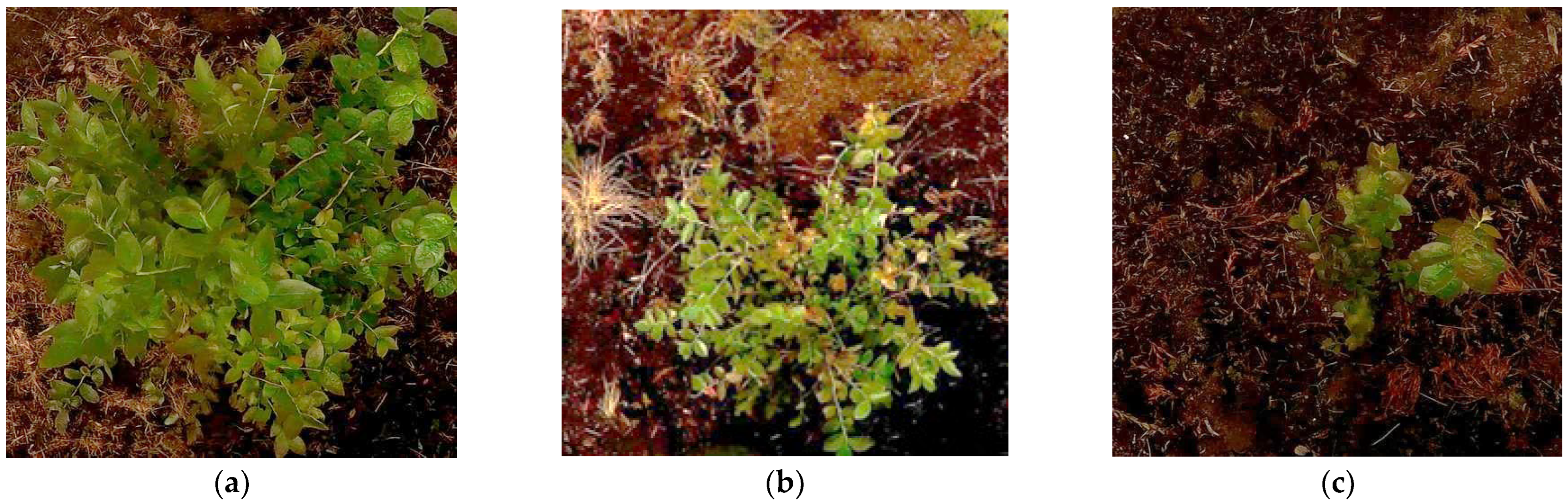
Figure 4a		0.7959	301 K	1.5704	65 K	0.4040	749 K	0.3658	556 K	49.24	149	76.71	754
Figure 4b		0.6872	359 K	1.2164	88 K	0.4352	728 K	0.6226	304 K	36.67	103	48.81	244
Figure 4c		0.6437	401 K	1.0613	89 K	0.3535	1151 K	0.6277	402 K	45.08	187	40.86	350
Average metric value:						0.3976	876 K	0.5387	421 K

¹ CHI metric values are rounded to the nearest thousand.

presents a comparative analysis of clustering performance before and after applying adaptive hue-based filtering in the HSL color space, for three plant sizes (large, medium, and small), as illustrated in Figure 4a–c. After filtering, both metrics generally show improved clustering quality, with the DBI metrics decreasing and the CHI metrics increasing for both K-means and GMM, showing that the adaptive hue-based filtering leads to more compact clusters with greater separation.

In Table 2, the row corresponding to Figure 4a, the DBI for K-means decreases by 49.24%, while the CHI improves by 149%, indicating significant improvements in cluster compactness and separation. Similar trends are observed for medium-sized and small plants, with DBI reductions of up to 76.71% and CHI enhancements reaching 754% for GMM, demonstrating that adaptive hue filtering effectively enhances clustering performance for both algorithms across different plant sizes. Notably, K-means consistently outperforms GMM, as evidenced by superior DBI and CHI improvements. The average metric values in Table 2 confirm that K-means provides the most effective plant cluster identification, a finding further supported by the clustering quality improvement visualized in Figure 6. Based on these results, we use the K-means algorithm in subsequent processing stages, including further plant cluster refinement and NDVI calculation. From Figure 6, we also observe that even after applying adaptive hue-based filtering in the HSL color space, some non-plant green regions, such as weeds and grass, may still be included within the plant bush cluster.

To further enhance the segmentation quality and exclude these non-plant areas, a DBI score-based filtering method is implemented. This method relies on adaptive pixel-wise average distance calculation to refine the plant cluster. First, using Equation (8), the average distance ($\overline{\mathrm{D}}\left(\mathrm{i}\right)$) for each pixel ($\mathrm{i}$) within the plant cluster is calculated, where $\mathrm{D}\left(\mathrm{i},\mathrm{j}\right)$ represents the Euclidean distance between pixels $\mathrm{i}$ and $\mathrm{j}$.

$$\overline{\mathrm{D}}\left(\mathrm{i}\right)={\displaystyle \frac{1}{\mathrm{N}}}{\sum }_{\mathrm{j}=1}^{\mathrm{N}}\mathrm{D}\left(\mathrm{i},\mathrm{j}\right)$$

(8)

After calculating the average distance for each pixel, we discard outlier pixels that deviate from the dense structure typical of the plant bush cluster. This approach is based on the observation that plant bush pixels are generally more compactly arranged, whereas non-plant green areas, such as grass or weeds, tend to be more dispersed, especially in top-down images. By excluding pixels with larger average distances, the process refines plant bush identification and improves clustering precision.

To determine the optimal percentile threshold for removing non-plant pixels, we employed the DBI metric that balances intra-cluster compactness with inter-cluster separation. The DBI, calculated after applying adaptive hue-based filtering in the HSL color space, helps to set an adaptive percentile threshold for outlier removal. Clusters with lower DBI scores, indicating well-formed, compact clusters, require a higher percentile threshold, while those with higher DBI scores, suggesting more diffuse clusters, use a stricter threshold. This adaptive threshold selection ensures the final clustering accurately represents the plant structure, excluding dispersed non-plant areas. The adaptive percentile selection method is shown in Equation (9), where ${\mathrm{P}}_{\mathrm{threshold}}$ is the calculated adaptive percentile threshold, and ${\mathrm{P}}_{\min }$ and ${\mathrm{P}}_{\max }$ define the lower (i.e., 85) and upper (i.e., 95) bounds of the average pixel distance percentile range. The threshold adapts based on the current DBI score ($\mathrm{DBI}$) as well as the minimum (${\mathrm{DBI}}_{\min }$) and maximum (${\mathrm{DBI}}_{\max }$) DBI values in the dataset. Based on the position of the current DBI score within this range the percentile threshold adjusts dynamically according to the cluster quality, ensuring more accurate plant bush cluster refinement. This adaptive mechanism enhances clustering precision by effectively distinguishing between tightly packed plant data and dispersed non-plant regions, without compromising important plant information.

$${\mathrm{P}}_{\mathrm{threshold}}={\mathrm{P}}_{\min }+\left({\displaystyle \frac{\mathrm{DBI}-{\mathrm{DBI}}_{\min }}{{\mathrm{DBI}}_{\max }-{\mathrm{DBI}}_{\min }}}\right)\times \left({\mathrm{P}}_{\max }-{\mathrm{P}}_{\min }\right)$$

(9)

Figure 7 presents the results of the adaptive average distance-based filtering process applied to the plant clusters (K-means) obtained from the adaptive hue-based filtering in the HSL space, i.e., Figure 6a–c. Specifically, the first column of Figure 7a,d,g corresponds to the plant cluster shown in Figure 6a, the second column (b,e,h) corresponds to Figure 6b, and the third column (c,f,i) corresponds to Figure 6c. The first row of Figure 7a–c shows histograms of pixel-to-pixel average distance distributions with the respective percentile cut-off points used in filtering. The second row (d,e,f) displays the refined plant clusters after filtering, while the third row (g,h,i) presents the final bounding boxes encapsulating these clusters.

Figure 7 demonstrates that after applying adaptive distance-based filtering, plant clusters of varying sizes are effectively identified, resulting in improved clarity and accuracy in cluster identification. The enhancements in cluster identification are particularly evident when comparing the results to Figure 6a–c, as both figures represent the same plant images, with the updated clustering process offering clearer distinctions.

2.3. NDVI Computation

The NDVI values for each pixel were calculated using Equation (10), which is adapted from a formula developed by Costa et al. (2020) [39].

$$\mathrm{vNDVI}=0.5268\times \left({\mathrm{red}}^{-0.1294}\times {\mathrm{green}}^{0.3389}\times {\mathrm{blue}}^{-0.3118}\right)$$

(10)

Genetic algorithms were applied to optimize the scaling factor and specific weight exponents for each RGB color channel, enabling effective approximation of NDVI values from RGB images. Each channel was normalized to scale the pixel intensities within the range (0, 1). Using this formula, we calculate the NDVI values for each pixel within the plant cluster’s bounding box (Figure 7g–i), and the average NDVI of these values provides a single NDVI estimate per plant. To prevent calculation errors, zero-value pixels encountered during normalization were replaced with a small constant (0.1).

Table 3. Sample data for plant bush clusters and their corresponding NDVI values.

Plant Custer 1	Bounding Box Coordinates		NDVI
	Min (x, y)	Max (x, y)
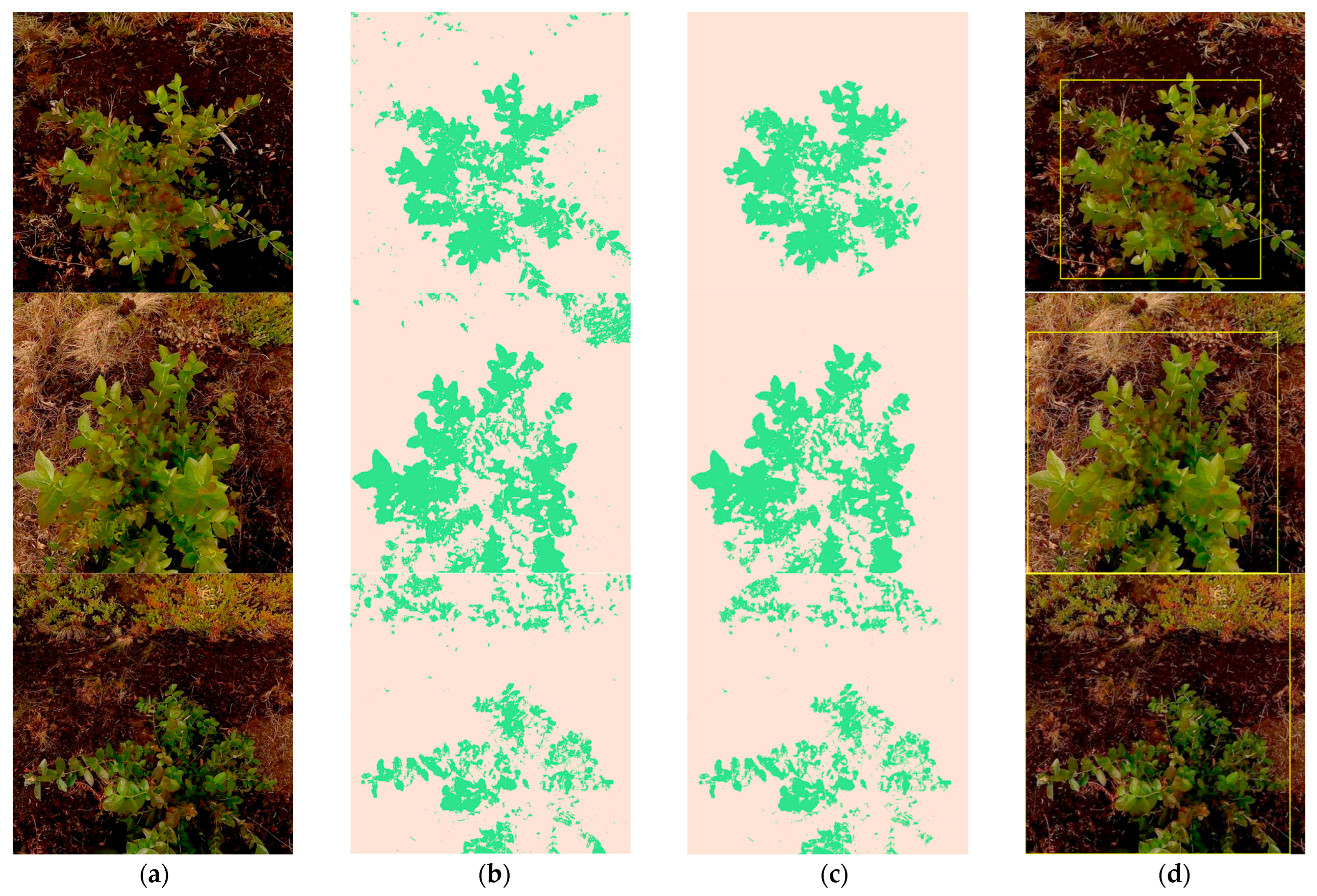
P009 (Figure 7g)	(11, 31)	(491, 474)	0.9218
P006 (Figure 7h)	(92, 123)	(468, 479)	0.7515
P050 (Figure 7i)	(217, 162)	(428, 357)	0.7743

¹ The plant clusters are identified by image IDs (e.g., P009, P006) linked to NDVI computation.

presents sample data for each plant cluster, including bounding box coordinates (minimum and maximum), and the computed NDVI values, corresponding to the plant clusters shown in Figure 7g–i.

2.4. Deep Learning Model Development

To predict NDVI values from plant bush clusters, a convolutional neural network (CNN) was developed, structured to effectively extract features from plant bush clusters, which were resized to 350 by 350 pixels, followed by fully connected (FC) layers to predict the final regression output.

2.4.1. Model Architecture

Predicting NDVI values from RGB images requires capturing spatially complex, non-linear relationships that traditional statistical methods struggle to model. CNNs, followed by FC layers, were chosen for their capacity to process spatial hierarchies in image data, effectively recognizing fine-grained details and patterns associated with plant bush clusters and their correlation to vegetation health.

Figure 8 illustrates the architecture of the CNN model designed for NDVI prediction. The model processes the input image through a series of layers that progressively extract, refine, and learn hierarchical features. The first stage consists of three convolutional layers (conv1, conv2, conv3) that progressively learn low- to high-level image features. The first two convolutional layers (conv1, conv2) are followed by batch normalization to stabilize the learning process and ensure efficient gradient flow, improving the model’s convergence during training. The output channels for these three layers are 32, 64, and 128, respectively, supporting the extraction of more complex features as the network deepens. The convolutional layers use a kernel size of (3, 3), stride of 2, and padding of 1, allowing for effective down-sampling of feature maps while preserving important spatial information.

After conv2 and conv3, max pooling layers with a kernel size of (3, 3), stride of 2, and padding of 0 are applied to further reduce the spatial dimensions, while retaining the most significant features for subsequent layers. Following the convolutional layers, the output feature maps are flattened into a one-dimensional vector and passed through three fully connected (FC) layers (fc1, fc2, fc3). The neuron counts in these layers decrease progressively from 12,800 to 512 to 32, enabling the model to refine its representation of the learned features. The final FC layer produces a single scalar output, which represents the predicted NDVI value.

Dropout regularization with a probability of 0.1 is applied to the fc1 and fc2 layers, reducing the risk of overfitting by randomly deactivating neurons during training. This ensures better generalization by preventing the model from becoming too reliant on any specific neuron during learning. The overall workflow of the model begins with the CNN layers, which extract and down-sample image features, followed by max pooling layers that further reduce the spatial dimensions. The FC layers then process these reduced features to produce the final NDVI prediction.

2.4.2. Model Training and Evaluation

The dataset was prepared by mapping the plant clusters’ location and their corresponding NDVI values. A custom dataset class loads and preprocesses images by resizing them to 350 × 350 pixels and normalizing pixel values to a range of 0 to 1. The dataset is divided into training, validation, and test sets with ratios of 70%, 15%, and 15%, respectively. To ensure reproducibility, a fixed random seed is used. PyTorch’s DataLoader enables efficient batch processing with a batch size of 5, supporting effective model generalization through iterative dataset loading and shuffling.

We train our model using an NVIDIA Quadro M5000 GPU with 8 GB of memory, on a system running Windows 11 Professional for Workstations. The hardware includes an Intel Xeon E5-1630 v4 (Intel Corporation, Santa Clara, CA, USA) processor (3.70 GHz, 4 cores, 8 logical processors) and 96 GB of physical RAM, ensuring robust computational support for the training process. The model was trained for a total of 300 epochs and saved the best model state based on the minimum validation loss. The mean squared error (MSE) loss function, in Equation (11), is used as the objective measure for training. This function calculates the average squared difference between the predicted NDVI values (${\widehat{\mathrm{y}}}_{\mathrm{i}}$), and the actual values (${\mathrm{y}}_{\mathrm{i}}$), where $\mathrm{N}$ represents the total number of data points. By minimizing the MSE, the model effectively reduces prediction errors, ensuring that predicted NDVI values closely approximate the ground truth, thereby enhancing overall model accuracy.

$$\mathrm{MSE}={\displaystyle \frac{1}{\mathrm{N}}}\sum _{\mathrm{i}=1}^{\mathrm{N}}{\left({\mathrm{y}}_{\mathrm{i}}-{\widehat{\mathrm{y}}}_{\mathrm{i}}\right)}^2$$

(11)

The Rectified Linear Unit (ReLU) activation function (Equation (12)) is applied after each convolutional and FC layer, except the final output layer (fc3), to introduce non-linearity. This activation enhances the model’s ability to capture complex relationships between image features and NDVI values, while promoting efficient gradient propagation and mitigating the vanishing gradient problem.

$$\mathrm{f}\left(\mathrm{x}\right)=\max \left(0,\mathrm{x}\right)$$

(12)

Dropout and L2 regularization were applied to reduce overfitting. Dropout stochastically deactivates neurons during training, preventing reliance on specific neurons. L2 regularization (Equation (13)), controlled by the weight decay factor $\mathsf{\lambda }$, penalizes large model weights and thus encourages lower model complexity. The regularization hyperparameter $\mathsf{\lambda }$ i.e., the weight decay factor (1 × 10⁻⁵) that controls the strength of the penalty on the weights, helps to prevent overfitting by discouraging overly complex models. The term ${\mathrm{w}}_{\mathrm{j}}^2$ represents the square of the weight ${\mathrm{w}}_{\mathrm{j}}$, for each model parameter j, contributing to the L2 regularization component in the total loss function.

$${\mathrm{Loss}}_{\mathrm{total}}=\mathrm{MSE}+\mathsf{\lambda }\sum _{\mathrm{j}}{\mathrm{w}}_{\mathrm{j}}^2$$

(13)

An Adam optimizer with a learning rate (η = 1 × 10⁻⁵) was employed to ensure stable learning and minimize performance fluctuations, thus promoting consistent convergence during training. This CNN architecture, in conjunction with a well-defined training and evaluation protocol, forms a robust system capable of accurately predicting NDVI values from individual plant bush cluster images.

3. Results and Discussion

In this study, we developed and evaluated a method for NDVI prediction that involved several key stages, i.e., from initial plant bush cluster identification to CNN-based NDVI regression (Figure 2). In the following sections, we provide a detailed overview of the results and discuss each major step of the methodology.

3.1. Plant Bush Cluster Identification

We develop a multi-stage method combining clustering, HSL color transformation, and adaptive filtering guided by the DBI metric to remove non-plant pixels while preserving compact plant clusters (Figure 7).

Initially, K-means and GMM clustering algorithms were applied to distinguish plant from non-plant regions (Figure 5). However, challenges in segmentation within the RGB color space (Figure 4), particularly the overlap in pixel values of plant and non-plant regions, required further refinement. To address this, we employ HSL transformation and adaptive hue-based filtering (Equation (4) and (5)) before clustering and get better isolated plant clusters (Figure 6). By dynamically defining the lower and upper bounds of the hue channel, the distinction between plant regions is improved, while dark or overly bright areas, which do not accurately represent the plant bush cluster, are excluded. The average DBI and CHI cluster metrics, presented in Figure 9 below, illustrate the performance of both algorithms before and after the application of the HSL transformation and adaptive hue filtering.

The results clearly demonstrate that both clustering algorithms yield significant improvements, with K-means outperforming GMM, as evidenced by both the DBI and CHI values.

Despite the improvements in clustering, the plant bush clusters still contain regions that do not belong to the plant, as observed in earlier figures (Figure 6). We further refine the plant bush cluster, and we focus exclusively on the K-means algorithm, given its better performance in the previous steps. An adaptive pixel-to-pixel average-distance-based filtering technique was then introduced to remove non-plant regions, guided by the DBI cluster value (Equations (8) and (9)). This value informed the selection of an adaptive percentile threshold for outlier removal, allowing for the exclusion of pixels with significantly high average distances, typically associated with diffuse non-plant areas, such as grass or weeds. The refined clustering results are shown earlier in Figure 7, where the final bounding boxes around the plant clusters highlight the quality of this multi-stage approach. Moreover, the minimum and maximum percentile thresholds (${\mathrm{P}}_{\min }$ = 85, ${\mathrm{P}}_{\max }$ = 95) applied in this study (Equation (9)) can be adjusted to achieve more refined clustering, particularly by lowering the ${\mathrm{P}}_{\min }$.

However, this method faces challenges when non-plant regions dominate the image. As shown in Figure 10, the clustering approach struggles to find the optimal cluster in such cases. Three types of results are presented—accurately identified clusters, slightly overestimated clusters, and highly overestimated clusters—which are shown in the first, second, and third rows of Figure 10, respectively.

Despite a few instances of slight or highly overestimated clusters, our proposed method effectively identified all plant regions, with no plant clusters left undetected.

3.2. Model Performance Evaluation

After successfully identifying individual plant clusters, NDVI values were calculated for each plant. The best-performing CNN model was saved based on the lowest validation loss, achieved at epoch 292 out of 300. The training and validation loss curves are presented in Figure 11.

Our model’s training and validation MSE losses were 0.0074 and 0.0044, respectively. After testing, the model achieved an MSE of 0.0021, a mean absolute error (MAE) of 0.0369, and a mean percentage error (MPE) of 4.5851. These metrics indicate high accuracy in NDVI prediction, as shown in Figure 12, which presents both the predicted data points and percentage error distribution across the test set.

The consistent trend in low percentage errors reflects the model’s robust performance in estimating NDVI values closely aligned with the actual measurements. The low MSE (0.0021), MAE (0.0369), and MPE (4.5851) highlight its accuracy and reliability in NDVI estimation tasks. These quantitative results are further supported by a visual comparison (Figure 12) that reveals close alignment between predicted and actual NDVI values. Overall, the evaluation highlights the CNN model’s ability to capture complex spectral and textural information from RGB images, enabling accurate NDVI predictions. This capability underscores the model’s potential for real-world precision agricultural applications, where precise NDVI estimation can play a critical role in plant health assessment and crop management.

4. Conclusions

This study presents a novel method for blueberry plant cluster identification and NDVI estimation using RGB images, combining clustering techniques with a CNN model to achieve precise NDVI predictions. Our model achieved high accuracy with a MSE of 0.0021, MAE of 0.0369, and MPE of 4.5851, demonstrating its reliability for NDVI estimation with a promising alternative for costly multispectral sensors. By leveraging RGB data alone, this approach provides a cost-effective alternative, making precision agricultural applications accessible on a larger scale, particularly for small farms. The ability to compute plant-specific NDVI values enables more accurate and targeted decision-making, such as precise fertilization and pesticide application. Moreover, the adaptive filtering and outlier removal processes make this methodology applicable to other similar plants by adjusting parameters specific to each plant.

Future work will focus on integrating this model with the agrobotic platform (Figure 1) and combining it with our previously developed blueberry root collar detection model [45]. This integration aims to support precision agriculture practices, such as targeted fertilization, optimized pesticide application, and improved crop management—ultimately enhancing resource efficiency, productivity, and environmental sustainability in agriculture.

References

- Foley, J.A.; Ramankutty, N.; Brauman, K.A.; Cassidy, E.S.; Gerber, J.S.; Johnston, M.; Mueller, N.D.; O’Connell, C.; Ray, D.K.; West, P.C.; et al. Solutions for a Cultivated Planet. Nature 2011, 478, 337–342. [Google Scholar] [CrossRef] [PubMed]
- Blesh, J.; Hoey, L.; Jones, A.D.; Friedmann, H.; Perfecto, I. Development Pathways toward “Zero Hunger”. World Dev. 2019, 118, 1–14. [Google Scholar] [CrossRef]
- Zhang, N.; Wang, M.; Wang, N. Precision Agriculture a Worldwide Overview. Comput. Electron. Agric. 2002, 36, 113–132. [Google Scholar] [CrossRef]
- Gebbers, R.; Adamchuk, V.I. Precision Agriculture and Food Security. Science 2010, 327, 828–831. [Google Scholar] [CrossRef] [PubMed]
- Talebpour, B.; Türker, U.; Yegül, U. The Role of Precision Agriculture in the Promotion of Food Security. Int. J. Agric. Food Res. 2015, 4, 1–23. [Google Scholar] [CrossRef]
- Kriegler, F.J.; Malila, W.A.; Nalepka, R.F.; Richardson, W. Preprocessing Transformations and Their Effects on Multispectral Recognition. In Proceedings of the Sixth International Symposium on Remote Sensing of Environment, Ann Arbor, MI, USA, 13–16 October 1969; Volume II, p. 97. [Google Scholar]
- Rouse, J.W.; Haas, R.H.; Schell, J.A.; Deering, D.W. Monitoring Vegetation Systems in the Great Plains with ERTS. NASA Spec. Publ. 1974, 351, 309. [Google Scholar]
- Veloso, A.; Mermoz, S.; Bouvet, A.; Le Toan, T.; Planells, M.; Dejoux, J.-F.; Ceschia, E. Understanding the Temporal Behavior of Crops Using Sentinel-1 and Sentinel-2-like Data for Agricultural Applications. Remote Sens. Env. 2017, 199, 415–426. [Google Scholar] [CrossRef]
- Tucker, C.J. Red and Photographic Infrared Linear Combinations for Monitoring Vegetation. Remote Sens. Env. 1979, 8, 127–150. [Google Scholar] [CrossRef]
- King, M.D.; Platnick, S.; Menzel, W.P.; Ackerman, S.A.; Hubanks, P.A. Spatial and Temporal Distribution of Clouds Observed by MODIS Onboard the Terra and Aqua Satellites. IEEE Trans. Geosci. Remote Sens. 2013, 51, 3826–3852. [Google Scholar] [CrossRef]
- Pelta, R.; Beeri, O.; Tarshish, R.; Shilo, T. Sentinel-1 to NDVI for Agricultural Fields Using Hyperlocal Dynamic Machine Learning Approach. Remote Sens. 2022, 14, 2600. [Google Scholar] [CrossRef]
- Berni, J.; Zarco-Tejada, P.J.; Suarez, L.; Fereres, E. Thermal and Narrowband Multispectral Remote Sensing for Vegetation Monitoring from an Unmanned Aerial Vehicle. IEEE Trans. Geosci. Remote Sens. 2009, 47, 722–738. [Google Scholar] [CrossRef]
- Anderson, K.; Gaston, K.J. Lightweight Unmanned Aerial Vehicles Will Revolutionize Spatial Ecology. Front. Ecol. Env. 2013, 11, 138–146. [Google Scholar] [CrossRef]
- Tsouros, D.C.; Bibi, S.; Sarigiannidis, P.G. A Review on UAV-Based Applications for Precision Agriculture. Information 2019, 10, 349. [Google Scholar] [CrossRef]
- Radoglou-Grammatikis, P.; Sarigiannidis, P.; Lagkas, T.; Moscholios, I. A Compilation of UAV Applications for Precision Agriculture. Comput. Netw. 2020, 172, 107148. [Google Scholar] [CrossRef]
- Pedersen, S.M.; Lind, K.M. Precision Agriculture—From Mapping to Site-Specific Application. In Precision Agriculture: Technology and Economic Perspectives; Marcus, P.S., Lind, K.M., Eds.; Springer International Publishing: Cham, Switzerland, 2017; pp. 1–20. [Google Scholar] [CrossRef]
- Kendall, H.; Clark, B.; Li, W.; Jin, S.; Jones, G.D.; Chen, J.; Taylor, J.; Li, Z.; Frewer, L.J. Precision Agriculture Technology Adoption: A Qualitative Study of Small-Scale Commercial “Family Farms” Located in the North China Plain. Precis. Agric. 2022, 23, 319–351. [Google Scholar] [CrossRef]
- Bai, A.; Kovách, I.; Czibere, I.; Megyesi, B.; Balogh, P. Examining the Adoption of Drones and Categorisation of Precision Elements among Hungarian Precision Farmers Using a Trans-Theoretical Model. Drones 2022, 6, 200. [Google Scholar] [CrossRef]
- Radočaj, D.; Šiljeg, A.; Marinović, R.; Jurišić, M. State of Major Vegetation Indices in Precision Agriculture Studies Indexed in Web of Science: A Review. Agriculture 2023, 13, 707. [Google Scholar] [CrossRef]
- Pallottino, F.; Antonucci, F.; Costa, C.; Bisaglia, C.; Figorilli, S.; Menesatti, P. Optoelectronic Proximal Sensing Vehicle-Mounted Technologies in Precision Agriculture: A Review. Comput. Electron. Agric. 2019, 162, 859–873. [Google Scholar] [CrossRef]
- Lowder, S.K.; Sánchez, M.V.; Bertini, R. Which Farms Feed the World and Has Farmland Become More Concentrated? World Dev. 2021, 142, 105455. [Google Scholar] [CrossRef]
- International Food Policy Research Institute. Global Food Policy Report; International Food Policy Research Institute: Washington, DC, USA, 2018; Volume 10, p. 9780896292970. [Google Scholar]
- Ricciardi, V.; Ramankutty, N.; Mehrabi, Z.; Jarvis, L.; Chookolingo, B. How Much of the World’s Food Do Smallholders Produce? Glob. Food Sec. 2018, 17, 64–72. [Google Scholar] [CrossRef]
- Guiomar, N.; Godinho, S.; Pinto-Correia, T.; Almeida, M.; Bartolini, F.; Bezák, P.; Biró, M.; Bjørkhaug, H.; Bojnec, Š.; Brunori, G.; et al. Typology and Distribution of Small Farms in Europe: Towards a Better Picture. Land. Use Policy 2018, 75, 784–798. [Google Scholar] [CrossRef]
- Tisenkopfs, T.; Adamsone-Fiskovica, A.; Kilis, E.; Šūmane, S.; Grivins, M.; Pinto-Correia, T.; Bjørkhaug, H. Territorial Fitting of Small Farms in Europe. Glob. Food Sec. 2020, 26, 100425. [Google Scholar] [CrossRef]
- Parrot. Parrot Sequoia+. Available online: https://www.parrot.com/en/shop/accessories-spare-parts/other-drones/sequoia (accessed on 15 October 2024).
- Drones, S.S. Sentera 6x Thermal. Available online: https://senterasensors.com/hardware/sensors/6x/ (accessed on 15 October 2024).
- AgEagle Aerial Systems Inc. Altum-PT. Available online: https://ageagle.com/drone-sensors/altum-pt-camera/ (accessed on 15 October 2024).
- AgEagle Aerial Systems Inc. RedEdge-P. Available online: https://ageagle.com/drone-sensors/rededge-p-high-res-multispectral-camera/ (accessed on 15 October 2024).
- SAL Engineering. MAIA S2. Available online: https://www.spectralcam.com/maia-tech-2/ (accessed on 15 October 2024).
- SILIOS Technologies. Toucan. Available online: https://www.silios.com/toucan-camera (accessed on 15 October 2024).
- Agrowing Ltd. A7Rxx Quad. Available online: https://agrowing.com/products/alpha-7rxxx-quad/ (accessed on 15 October 2024).
- Mizik, T. How Can Precision Farming Work on a Small Scale? A Systematic Literature Review. Precis. Agric. 2023, 24, 384–406. [Google Scholar] [CrossRef]
- Stamford, J.D.; Vialet-Chabrand, S.; Cameron, I.; Lawson, T. Development of an Accurate Low Cost NDVI Imaging System for Assessing Plant Health. Plant Methods 2023, 19, 9. [Google Scholar] [CrossRef]
- Cucho-Padin, G.; Loayza, H.; Palacios, S.; Balcazar, M.; Carbajal, M.; Quiroz, R. Development of Low-Cost Remote Sensing Tools and Methods for Supporting Smallholder Agriculture. Appl. Geomat. 2020, 12, 247–263. [Google Scholar] [CrossRef]
- Hobbs, S.; Lambert, A.; Ryan, M.J.; Paull, D.J. Preparing for Space: Increasing Technical Readiness of Low-Cost High-Performance Remote Sensing Using High-Altitude Ballooning. Adv. Space Res. 2023, 71, 1034–1044. [Google Scholar] [CrossRef]
- Holman, F.H.; Riche, A.B.; Castle, M.; Wooster, M.J.; Hawkesford, M.J. Radiometric Calibration of ‘Commercial off the Shelf’ Cameras for UAV-Based High-Resolution Temporal Crop Phenotyping of Reflectance and NDVI. Remote Sens. 2019, 11, 1657. [Google Scholar] [CrossRef]
- Barrows, C.; Bulanon, D. Development of a Low-Cost Multispectral Camera for Aerial Crop Monitoring. J. Unmanned Veh. Syst. 2017, 5, 192–200. [Google Scholar] [CrossRef]
- Costa, L.; Nunes, L.; Ampatzidis, Y. A New Visible Band Index (VNDVI) for Estimating NDVI Values on RGB Images Utilizing Genetic Algorithms. Comput. Electron. Agric. 2020, 172, 105334. [Google Scholar] [CrossRef]
- Davidson, C.; Jaganathan, V.; Sivakumar, A.N.; Czarnecki, J.M.P.; Chowdhary, G. NDVI/NDRE Prediction from Standard RGB Aerial Imagery Using Deep Learning. Comput. Electron. Agric. 2022, 203, 107396. [Google Scholar] [CrossRef]
- Moscovini, L.; Ortenzi, L.; Pallottino, F.; Figorilli, S.; Violino, S.; Pane, C.; Capparella, V.; Vasta, S.; Costa, C. An Open-Source Machine-Learning Application for Predicting Pixel-to-Pixel NDVI Regression from RGB Calibrated Images. Comput. Electron. Agric. 2024, 216, 108536. [Google Scholar] [CrossRef]
- Farooque, A.A.; Afzaal, H.; Benlamri, R.; Al-Naemi, S.; MacDonald, E.; Abbas, F.; MacLeod, K.; Ali, H. Red-Green-Blue to Normalized Difference Vegetation Index Translation: A Robust and Inexpensive Approach for Vegetation Monitoring Using Machine Vision and Generative Adversarial Networks. Precis. Agric. 2023, 24, 1097–1115. [Google Scholar] [CrossRef]
- Jeong, U.; Jang, T.; Kim, D.; Cheong, E.J. Classification and Identification of Pinecone Mulching in Blueberry Cultivation Based on Crop Leaf Characteristics and Hyperspectral Data. Agronomy 2024, 14, 785. [Google Scholar] [CrossRef]
- Anku, K.E.; Percival, D.C.; Lada, R.; Heung, B.; Vankoughnett, M. Remote Estimation of Leaf Nitrogen Content, Leaf Area, and Berry Yield in Wild Blueberries. Front. Remote Sens. 2024, 5, 1414540. [Google Scholar] [CrossRef]
- Zaman, A.; Mahmoud, N.; Virro, I.; Liivapuu, O.; Lillerand, T.; Roy, K.; Olt, J. Learning with Small Data: A Novel Framework for Blueberry Root Collar Detection. In Proceedings of the 35th DAAAM International Symposium; Katalinic, B., Ed.; DAAAM International: Vienna, Austria, 24–25 October 2024. [Google Scholar]
- Mahmoud, N.T.A.; Virro, I.; Zaman, A.G.M.; Lillerand, T.; Chan, W.T.; Liivapuu, O.; Roy, K.; Olt, J. Robust Object Detection Under Smooth Perturbations in Precision Agriculture. AgriEngineering 2024, 6, 4570–4584. [Google Scholar] [CrossRef]
- Lillerand, T.; Virro, I.; Maksarov, V.V.; Olt, J. Granulometric Parameters of Solid Blueberry Fertilizers and Their Suitability for Precision Fertilization. Agronomy 2021, 11, 1576. [Google Scholar] [CrossRef]
- Virro, I.; Arak, M.; Maksarov, V.; Olt, J. Precision Fertilisation Technologies for Berry Plantation. Agronomy Research 2020, 18, 2797–2810. [Google Scholar] [CrossRef]
- Davies, D.L.; Bouldin, D.W. A Cluster Separation Measure. IEEE Trans. Pattern Anal. Mach. Intell. 1979, PAMI-1, 224–227. [Google Scholar] [CrossRef]
- Calinski, T.; Harabasz, J. A Dendrite Method for Cluster Analysis. Commun. Stat. Theory Methods 1974, 3, 1–27. [Google Scholar] [CrossRef]