1. Introduction
Several variables affect the performance of a crop within a single plot, which can be grouped into factors relating to the genotype of the crop installed, the environment that surrounds the crop, and the management practiced by those who manage the field. Therefore, on one hand, comprehensively treating an entire field for one limiting factor may not be the best way to optimize resource use or increase productivity; on the other hand, around a third of all soils are affected by the major global problem of soil degradation [
1]. Portugal is in the Mediterranean-Atlantic region, with edaphoclimatic conditions that allow a very high risk of soil erosion. There is a large annual precipitation variability (P; mm), only 4.2% of soils have a high cation exchange capacity (CEC), and most have a low organic matter content and are acidic. In addition to the heterogeneity of the regional scale, there is a great in-field diversity of natural soil conditions where 80% of it has moderate to high risk of erosion [
2,
3]. In addition, fodder crops mechanized operations usually performed with wet soils are responsible for the degradation of the physical soil structure. The agronomic management of agricultural fields carried out uniformly, with spatial variability evident, is economically and environmentally inefficient [
4,
5,
6]. The alternative is to adopt innovative resilient farming systems matching conventional tillage yields, facing the current climate-changing and production costs scenarios [
7,
8]. For this reason, site-specific management is important for enhancing crop productivity and increasing nutrient use efficiency [
5,
9].
Management zones (MZs) offer a solution to mapping the spatial pattern of soil variables and to isolate different problems and needs of different homogeneous areas in a single field. These different problems and needs may be nutritional or water deficiencies or other input management needs (mechanization, herbicide, phytosanitary treatment), which require different actions in each MZ. Although many observations are needed on different and varied variables, and it is a great challenge in terms of computing capacity, data management, and operationalization in the field [
10], it is important to find methodologies compatible in terms of cost-effectiveness that help farmers to delineate those homogeneous zones [
11]. At present, tools that employ geospatial information enabling detailed soil and crop mapping [
12], such as soil apparent electrical conductivity (ECa; mSm-1) [
13,
14] and remote sensing, stand as some of the most dependable techniques. These methods effectively characterize the spatial pattern of soil properties within fields [
13] and assess vegetation conditions [
15], contributing significantly to the concept of sustainable agriculture [
16].
ECa correlates with diverse physicochemical properties across a broad spectrum of soils at different depths [
17,
18] including compaction [
17,
19], sand, and clay content [
20]. This correlation enables the targeted management of specific areas concerning essential plant macro- and micro-nutrients [
21].
Remote sensing is extensively employed for pre-harvest crop yield prediction [
22], offering detailed spatial data on crop spectral characteristics. It detects variations in vegetation patterns, including emergence rates, leaf area index, and biomass [
23]. The optical remote sensing satellites that make up the Sentinel-2 constellation provide this type of spatial data at a resolution of 10 m, 20 m, and 60 m, depending on the bands, and a revisit period of only 5 days.
It was noted that there is a gap in previous research regarding land relief in the context of soil degradation and how to contribute further to the delineation of different MZs using soil and crop data. This paper aims to boost the importance of both in situ and remote evaluations and a farmer-scale field under no-till seeding (to minimize disturbance to the soil’s physical condition). To ensure result reliability, data spanning three years were compiled, and the cause and effect relationship with the meteorological year throughout this period was considered. At the present moment, although variable rate technologies (VRTs) are increasingly present in farm equipment solutions, how to define MZs still is a challenge considering the amount of variables that can be considered. The significance of this study lies in the increasing demand from farmers to understand methods enabling them to interpret georeferenced data, thus facilitating the demarcation process of MZs.
2. Materials and Methods
This study focused on a mixed fodder crop based on ryegrass under no-till. The materials and methods encompassed several key steps to comprehensively assess the impact of MZs on crop yield and resource use efficiency. The key steps of the procedure began with Step 1, involving the acquisition of soil spatial information, followed by meticulous pre-processing, interpretation, and spatial interpolation. Subsequently, in Step 2, MZs for soil characteristics were delineated using a combination of ECa measurements and soil analysis. Step 3 spanned over three years of gathering meteorological data and crop remote sensing measurements. These data underwent rigorous pre-processing, interpretation, and spatial-temporal clustering. In Step 4, site-specific crop MZs were delineated, leveraging a comprehensive dataset rich in information. This data set includes physical and chemical soil data; analyzed laboratory and other sensors; data on cultural management and vegetative vigor, collected by satellite; and local weather data.
2.1. Step 1
2.1.1. Experimental Field
The research took place over three years between October and May of 2020/21, 2021/22 and 2022/23 ((I), (II), and (III), respectively) in an irrigated area of 30 ha in Elvas, Alentejo region (Portugal) with the local coordinates 4706572.00 N; 784908.00 W. Plot boundaries (
Figure 1) were georeferenced using a portable Magellan receiver (Magellan Navigation Inc., model MobileMapper CX, San Dimas, CA, USA), with differential correction signal (DGPS), allowing positional accuracy of 0.15–0.20 m.
Climate, according to Köppen–Geiger is Csa and typically experiences hot and dry summers and cool and wet winters [
24]. As indicated by the World Meteorological Organization (WMO), they are the average values of various elements that characterize the climate, considering 30 years as sufficient and representative. Starting in the first year of each decade, the most recent period of reference is 1971–2000 and is called the Climatological Normal (CN) to the meteorological statistical results. The Portuguese Institute for Sea and Atmosphere (PISA) offers CNs’ information in Portugal, including Elvas station, about monthly and annual values of major climatic elements, mainly medium air temperature (Tm; °C) and P (
Table 1) [
25].
2.1.2. Soil Analyses and Survey
According to the FAO classification, the predominant soil of the field is a Luvisol that corresponds to Pag and Sr Mediterranean soil categories [
26]. Pag displays a brown to brownish or light grey hue, featuring sandy or loamy sandy composition, occasionally containing coarse quartz elements throughout its profile. Its structure lacks aggregates or exhibits weak fine granules. On the other hand, Sr exhibits a brown or reddish-brown color, typically with numerous coarse elements distributed throughout its profile, displaying a moderate or weak fine granular structure.
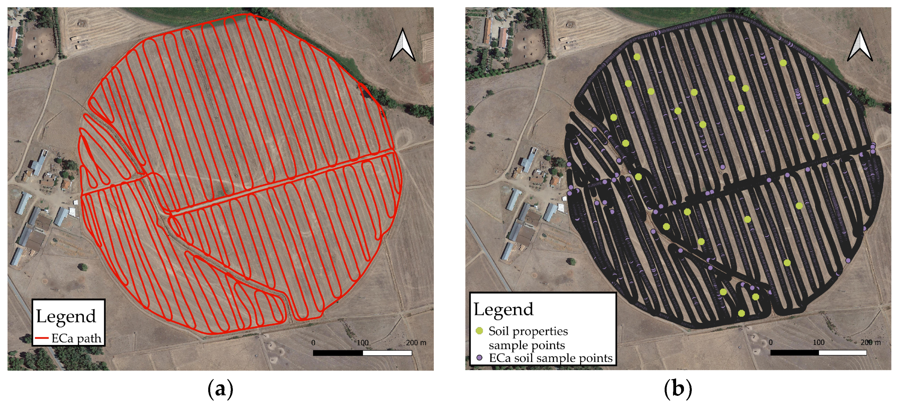
Soil monitoring was based on a preliminary evaluation of the field for ECa followed by in situ georeferenced evaluations. Soil ECa was performed at a depth of 0.50 m with an EM38 sensor (Geonics Limited, Mississauga, Ontario, Canada) with a Global Navigation Satellite System (GNSS) and a real-time kinematic (RTK) base station for soil topography. The sensor inside a cart was towed to an all-terrain vehicle (ATV) carried out in an A–B straight pattern of 12 m width and a forward speed of 10 km h
−1. To enhance the accuracy of SWAT passes and forward speed, the ATV was fitted with an assisted steering system, model EZ-Guide 250 (Trimble Navigation Limited, Sunnyvale, CA, USA) (
Figure 2a). A sum of 15,091 points was georeferenced, equivalent to roughly 473 ECa samples per hectare. In situ georeferenced evaluations based on the ECa map were performed with the same receiver described above to determine soil texture and properties (
Figure 2b).
The soil sampling procedure included the collection of a composite sample using an open-end soil probe at the 0–0.20 m layer. Subsequently, the samples were air-dried and sieved through a 2 mm mesh for the analysis of specific physical-chemical properties within the <2 mm fraction, such as particle size distribution (sand, silt, and clay; %), following ISO 11277:2020 standards [
27]; pH (H2O 1:2.5 suspension (p/v); soil organic matter (SOM; g kg
−1), following the Walkley–Black method [
28]; extractable phosphorus (P) (mg P
2O
5 kg
−1) and extractable potassium (K) (mg K
2O kg
−1) by the Egner–Riehm method [
29]; extractable magnesium (Mg) (mg Mg kg
−1) by 1 M ammonium acetate (pH 7); exchangeable calcium (Ca), magnesium (Mg
exc), potassium (K
exc), sodium (Na), and CEC (cmol (+) kg
−1), following ISO 11260:2018 [
30].
2.2. Step 2
2.2.1. Descriptive Statistics and Coefficient of Variation
Descriptive statistics including mean, minimum (Min), maximum (Max), and standard deviation (SD) and the coefficient of variation (CV) of the studied soil properties were delineated [
31,
32]. The relationships between the soil properties were evaluated by obtaining the values of the correlation coefficient and Student
t-tests for identification of significant differences.
2.2.2. Geostatistical Analysis
To assess the spatial variation pattern of the soil properties under study, a semi-variogram was calculated using Equation (1) by utilizing ArcGIS (version 2.9.3., ESRI, Inc., Redlands, CA, USA).
In this context: γ(h) denotes the semivariance corresponding to the lag distance (h), n (h) signifies the number of sample pairs separated by (h), z(Xa) represents the measured value of the sample at the sampling location (αth), and z(Xa + h) is the measured value of the sample at the location (h + αth). Various semi-variogram models, including stable, circular, Gaussian, exponential, and spherical, were calculated to identify the most suitable model for each soil property.
The cross-validation technique was employed to select the most suitable semi-variogram model for each of the soil properties under study. This involved a comparison between the predicted values obtained through kriging, using the semi-variogram model, and the actual measured values. Mean error (ME) was then computed for each model to identify the best-fitted one for each soil property. The model with the lowest ME value was considered the best, indicating the highest level of prediction accuracy (Equation (2)).
In this equation, n represents the number of observations for each case, z(xi, yi) denotes the observed soil property, z x (Xj, Yi) represents the estimated soil property, and (xi, yi) corresponds to the coordinates of the soil sample.
The values for various soil properties were extrapolated to unsampled locations for each property using the ordinary kriging (OK) method [
33]. OK was chosen due to its reliability among all prediction techniques based on ME [
34]. It is also the optimal unbiased method for cases where soil sample locations were randomly and sparsely chosen to predict soil property values at unsampled points. It also reduces the outliers’ impact as one of its most important benefits [
35]. While other methods exist for understanding spatial variability, semi-variograms and kriging stand out for their ability to quantify and model spatial dependence, providing more nuanced and reliable insights into the variability of datasets across space, namely understanding how closely located points relate to each other and the overall spatial trends; accommodating irregularly spaced data points, making it useful when dealing with datasets collected across varying spatial distributions; and offering a measure of confidence in the generated results.
2.2.3. PCA
To synthesize the main sources of data variation among correlated variables, principal component analysis (PCA) was performed. PCA is a multivariate analysis technique used for dimension reduction, using correlated variables to recombine and identify the orthogonal linear of the variables. For the PCA in this case, a correlation matrix containing the studied soil properties was used instead of a covariance matrix, resulting in a normalized PCA. The number of the principal components (PCs) had to be equivalent to the number of variables included in the analysis. Only PCs with high Eigenvalues were the best to represent the studied properties [
36]. In this study, the MZs were achieved by employing the scores of PCs with Eigenvalues exceeding 1 in the clustering analysis.
2.2.4. ISOcluster and Maximum Likelihood Classification
The final classified map was generated using an unsupervised classification technique on the sets of input layers that most influence the spatial variation of the soil. The classification was conducted using the ISO Cluster approach in ArcGIS (version 2.9.3., ESRI, Inc., Redlands, CA, USA). This algorithm arranges the data within the input rasters into a user-defined number of groups to generate signatures. These signatures are then employed in classifying the data via the “Maximum Likelihood Classifier” (MLC) function. The use of the ISO Cluster and Maximum Likelihood Classification tools in this study is justified by the fact that we have a series of input raster bands, which need to be classified in an unsupervised way. For this study, the number of groups was set at three (low, intermediate, and high potential) due to the practical need to delineate only a few homogeneous zones [
37,
38].
2.3. Step 3
2.3.1. Meteorological Survey
Daily meteorological data for Tm and P were recorded through the local meteorological station of the National Institute of Agricultural and Veterinary Research of Elvas, which is integrated into the national network of PISA meteorological stations.
The air temperature-sensitive element is a platinum resistance (PT100) duly calibrated by PISA and highly stable for resistance values, in the range of air temperatures possible at the Earth’s surface. Resistance variations are measured by an electronic circuit that presents a voltage output that is converted into degrees Celsius (°C) [
25]. The precipitation detection sensor used in the national network of meteorological stations is Vaisala’s DRD11 (Vaisala, Vantaa, Finland) [
25,
39].
In
Figure 3, the ombrothermic diagram gathers the data for Tm and P from the 3 years of the trial and the CN. This diagram excludes the month of October as it had only 2 days in the first year (I) and the month of May due to there being less than a decade’s worth of data for any of the trial years, with the crops already in their final stage.
2.3.2. Crop Itinerary and Survey
In the studied years sowing of a mixed fodder crop (
Table 2) under no-till took place in late-October to mid-November following irrigation and weed control, a glyphosate-based herbicide was applied.
During the sowing operation, an initial application of 28 kg/ha of nitrogen (N) fertilizer was administered. Along the crop cycle, the remaining N was applied as topdressing applications (
Table 3).
Table 4 displays the approximate dates of the agricultural operations conducted over the three years of the trial. The participatory farmer conducted all the field operations, and we monitored the processes.
According to [
40,
41] the base temperature (
Tbase) for
Lolium multiflorum L. is approximately 5 °C, and this value is considered the vegetative zero for the crop. In the case of
Trifolium resupinatum L., [
42] noted that the vegetative zero for the crop varies between 5.2 and 5.7 °C, with the base temperature value assumed to be 5 °C. This value was considered as the vegetative zero for the crop because forages are predominantly composed of ryegrass. The calculation of growing degree-days (GDD) aimed to predict the crops’ phenology for subsequently determining the potential number of harvests for various scenarios and adaptation measures considered. GDD were calculated for the reference period (1971–2000) (
Table 5), and the equation used for their determination was as follows (Equation (3)) [
43]:
where the maximum temperature (
Tmax) and minimum temperature (
Tmin) are obtained from meteorological stations, and the
Tbase constitutes a constant value for each crop. The crop development could be divided into three main phases: initial (L_ini), intermediate (L_dev), and final (L_mid).
2.3.3. Remote Sensing and Vegetation Indexes (VIs) Measurements
Cloud-free Sentinel-2 optical images, available from the European Space Agency, were selected and downloaded from ESA’s Copernicus Data Space [
45]. The images were captured on the closest available dates to the harvest moment (
Table 6). Data extraction was performed for the pixels of the experimental field.
Analyses were performed using Quantum GIS (QGIS) software (version 3.28.4., QGIS Development Team). Using the QGIS raster calculator, the Normalized Difference Vegetation Index (NDVI), Normalized difference red edge index (NDRE), and Normalized Difference Moisture Index (NDMI) were computed (
Table 7) [
46].
NDVI was computed from the 10 m spatial resolution Red (B04) and Near-Infrared (B08) spectral bands. NDRE, which measures chlorophyll levels in plants, is most effectively applied during the mid-to-late growing season, when the plants have matured and are nearing harvest readiness. At this point, other indices (such as NDVI) would be less effective to use. It is represented by a certain value calculated using a combination of a Near-InfraRed (B09) band and the RedEdge (B05) range between visible Red and NIR. The NDMI (Normalized Difference Moisture Index) was calculated to assess moisture levels in vegetation by utilizing a combination of near-infrared (B08) and short-wave infrared (B11) spectral bands. It serves as a dependable indicator of water stress in crops. Although colloquially NDMI is often compared with the Normalized Difference Water Index (NDWI), the two should be distinctly regarded as separate indices. NDMI (Gao’s version of NDWI) utilizes the NIR-SWIR combination to identify moisture content in leaves, whereas McFeeters’s NDWI employs the GREEN-NIR combination to accentuate water bodies and monitor their turbidity. We did not use the McFeeters’s NDWI for this study.
2.4. Step 4—Validation of Soil MZs by VI’s
The average values of the crop parameters were described using the mean, SD, and CV.
To facilitate the validation process of MZs based on soil and VIs, a global index (GI) was calculated for each parameter in the experimental field, as followed by [
37]. In this computation, a coefficient “1” was assigned to the highest parameter value among the set of 3 MZs. The values of the same parameter in the other two zones were converted into decimal fractions relative to this maximum value (referred to as relative value of each parameter; RV). This was determined by calculating the ratio between the value in question and the maximum value, as shown in Equation (4).
where: RV represents the relative value of each parameter; AV stands for the absolute value; Max.V denotes the maximum value; i signifies the location; j represents the homogeneous MZs; m is the total number of homogeneous MZs; k stands for the measured parameter; n signifies the number of locations of each j-k pair.
Following the computation of ratios for each zone and experimental field, the average value of the GI for each parameter within the experimental field was determined (Equation (5)).
where
RV represents the relative value of each parameter;
i signifies the location;
j represents the homogeneous MZs;
m is the total number of homogeneous MZs;
k stands for the measured parameter;
n signifies the number of locations of each
j-
k pair.
3. Results
3.1. Soil HMZs
3.1.1. Variability and Spatial Distribution of ECa and Altimetry
The descriptive statistics of soil ECa and altimetry are given in
Table 8. In 15091 sample points the average value of ECa was 27.33 millisiemens per meter (mSm
−1), within a range between 0.27 mSm
−1 e 62.62 mSm
−1.
The positioning sensor recorded an average altitude of 180.43 m above sea level, within a range of 173.15 m to 190.50 m.
Before performing geostatistical analysis, ECa soil and field altimetry values were log-transformed.
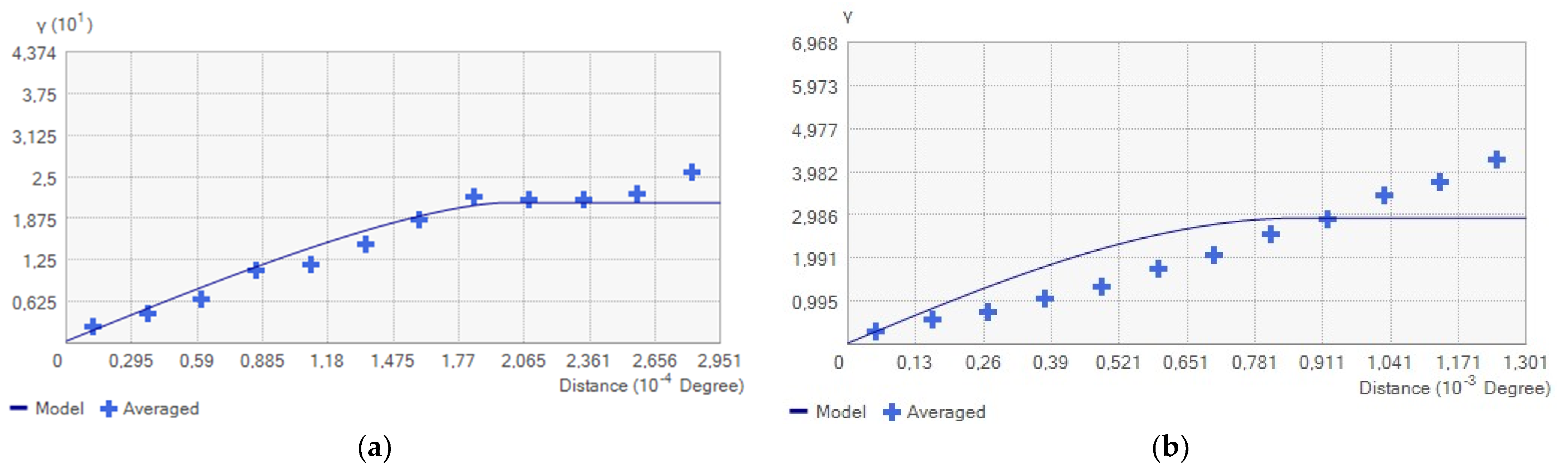
Table 9 and
Figure 4 show the parameters of the studied soil properties semi-variograms.
The cross-validation technique was employed to achieve the most precise predictions, aiming for the lowest ME values for the soil properties under study, as outlined in
Table 9. According to Shaddad et al. [
47], the lower ME values indicated that kriging predictions for soil properties closely aligned with the estimated values. Each studied soil properties’ mean square standardized error (MSSE) value ideally should be one. However, if the MSSE value deviated from one but remained within the tolerance range of 1 ± 3 (2/N)1/2, where N represented the number of soil samples, the model was deemed accurate. The tolerance range spanned from −0.999 to 1.000, as illustrated in
Table 9. All soil properties’ MSSE values fell within this range, signifying the high predictive accuracy of the semi-variogram models employed for these soil attributes.
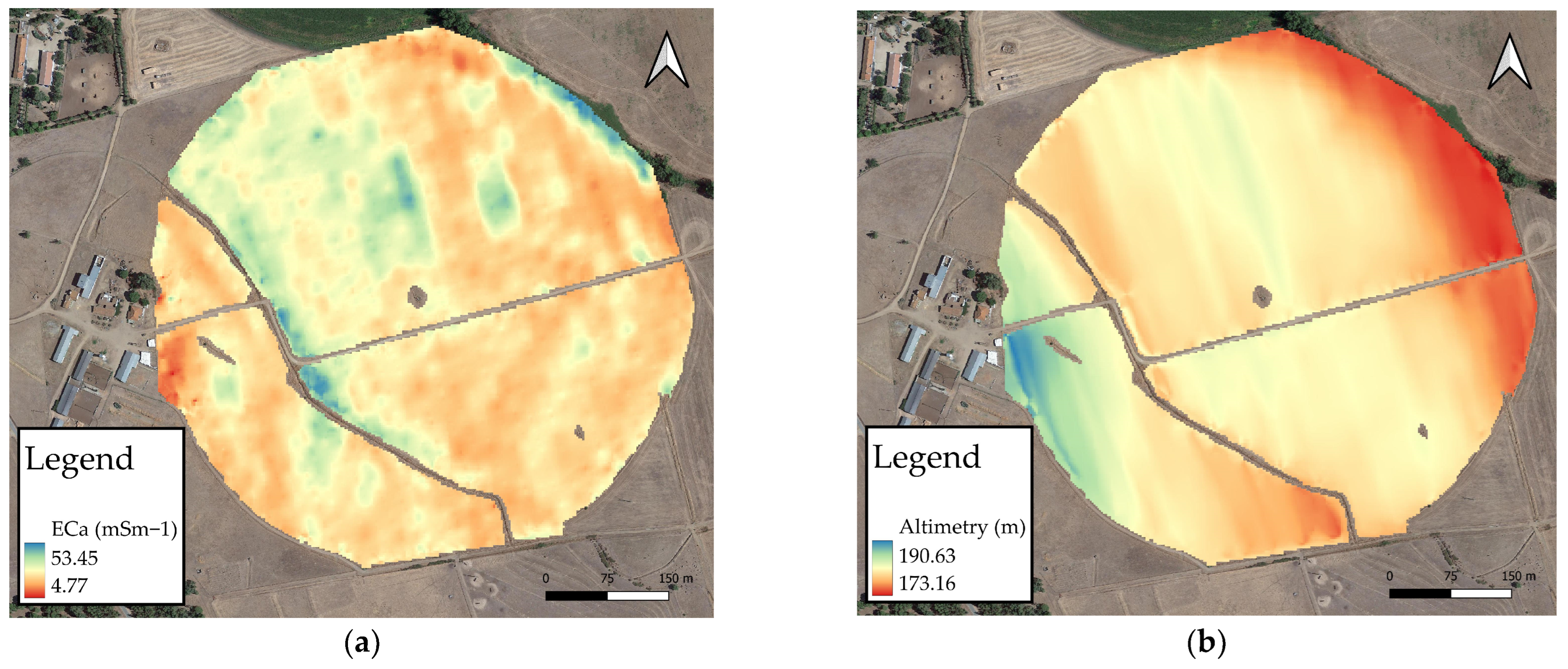
Figure 5 shows the distribution maps of the studied soil properties.
Significant insights into the nutrient content within the study area were acquired. These maps, generated through the OK technique, provide essential data for proposing site-specific nutrient management strategies. Leveraging this data can optimize output while minimizing input costs, thereby enhancing income through the implementation of best management practices.
3.1.2. Variability and Correlation of Soil Properties
The descriptive statistics of the studied soil properties are given in
Table 10. The soil of the study area has a range of sand between 61.2 and 79.1 g/kg. There is a tendency for a higher quantity of clay, ranging between 8.5 and 23.9 g/kg, compared to silt, which ranges between 8.6 and 16.9 g/kg. The study area tends to be slightly neutral, with an average pH of 6.8, within a range of 5.8 to 7.6. The mean SOM was 1.2 g/kg, with a maximum of 1.8 g/kg. According to the soil nutrient classification of Portugal [
48], the mean of SOM content was low in the study area, while the mean of P and K were very high and high, with a mean value of 218.6 mg P
2O
5/kg and 109.0 mg K
2O/kg, respectively. The average Mg value is 226.9 mg Mg kg
−1, which is classified as very high.
CEC has an average value of 7.9 cmol (+) kg−1, classifying it as low. The average value of Ca in the exchange complex is 5.3 cmol (+) kg−1, being classified as low, as are Kexc and Na, as they present values of 0.2 and 0.1 cmol (+) kg−1. Mgexc is classified as medium, as it presents an average value of 2.0 cmol (+) kg−1.
The lowest CV (1.2%) was for altimetry, while the highest CV (90.0%) was for K. According to Jakobsen [
49], the CV of the different soil properties ranged from low (<10%) to moderate (10 to 100%). Values of CV lower than 10% are sand (8.1%), pH (6.6%), and altimetry (1.2%).
The degree of correlation among the ten soil properties is shown in
Table 11.
3.1.3. Spatial Distribution of Soil Properties
Table 12 shows the parameters of the studied soil properties’ semi-variogram. Soil sand, silt, Mg
exc, and Na were best modelled by using circular models. While clay, Ca, and CEC were fitted best with exponential models, pH and K
exc were fitted best with Gaussian models and SOM fitted best with stable models.
To achieve highly accurate predictions with the lowest ME values for the soil properties under study, a cross-validation technique was performed (
Table 12). No spatial correlations were found for the parameters P, K, and Mg; therefore, spatial distribution maps for these parameters were not created. The possible models to use to create the semivariogram presented an average standard error (ASE) of 99.827% for P, 63.877% for K, and 70.738% for Mg.
3.1.4. PCA
Table 13 indicates that a significant correlation exists among most of the studied soil properties. PCA was conducted to synthesize and consolidate the variability observed in the ten studied variables. The number of resulting PCs equaled the number of variables included in the analysis. Only PCs with Eigenvalues surpassing 1 were retained for the final analysis, as a PC with an Eigenvalue greater than 1 explains more variance than an individual attribute, following the principle outlined by [
50]. As per this criterion, the first four PCs accounted for 99.34% of the total variability in the measured data, as detailed in
Table 13.
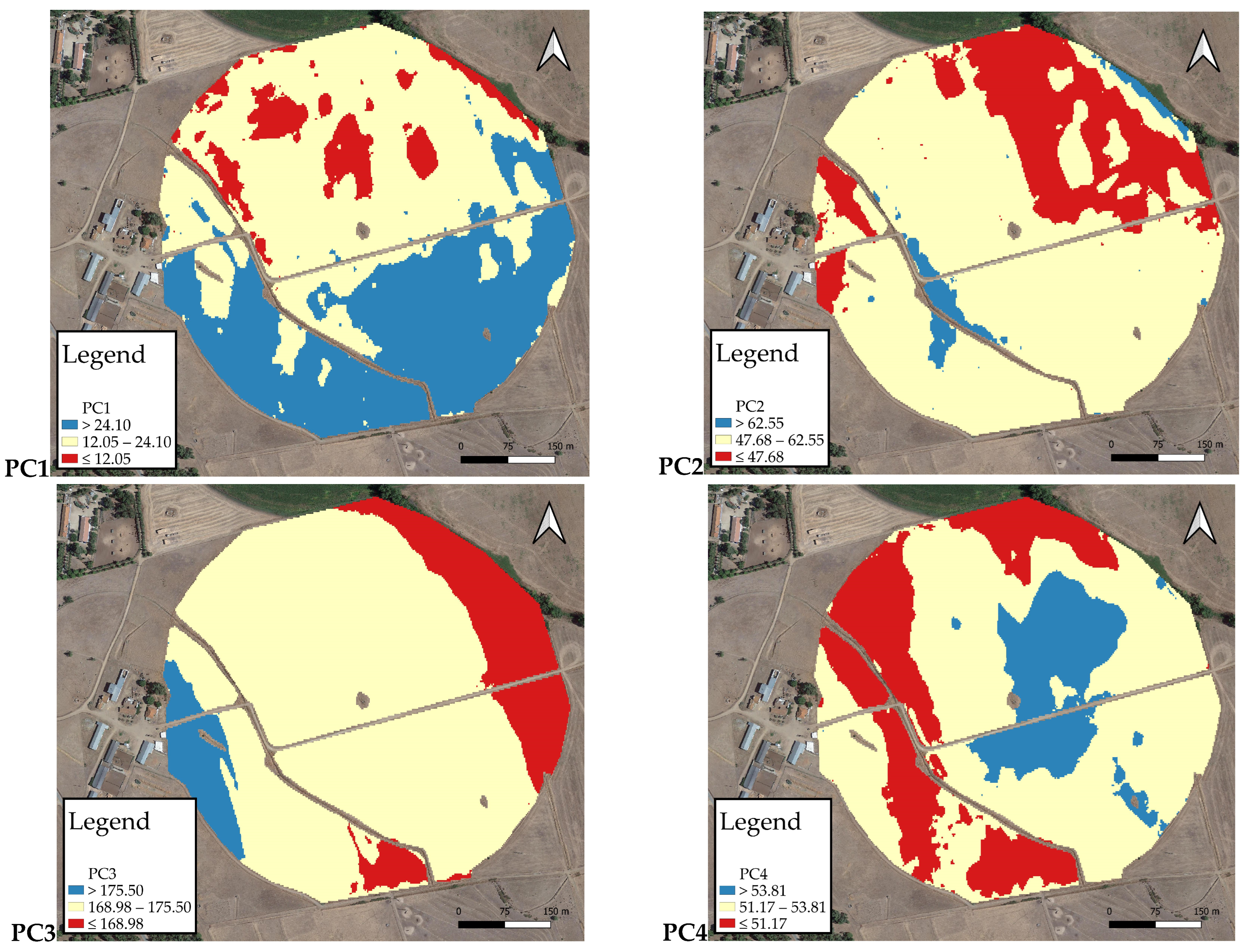
The most influential soil properties in PC1 are sand and ECa; in PC2 it is ECa; in PC3 it is altimetry; and in PC4 they are Ca and CEC (
Table 14).
Isolating the four PCs that explain the differences in soil properties, the maps are shown in
Figure 6.
PC1 explained 51.06% of the total variability, and it was dominated by sand and ECa. ECa and sand also influenced PC2, which explained 36.77% of the total variability, while PC3 explained 9.09% of the total variability and was controlled by altimetry. PC4 explained 2.43% of the variability and was affected by soil Ca and CEC.
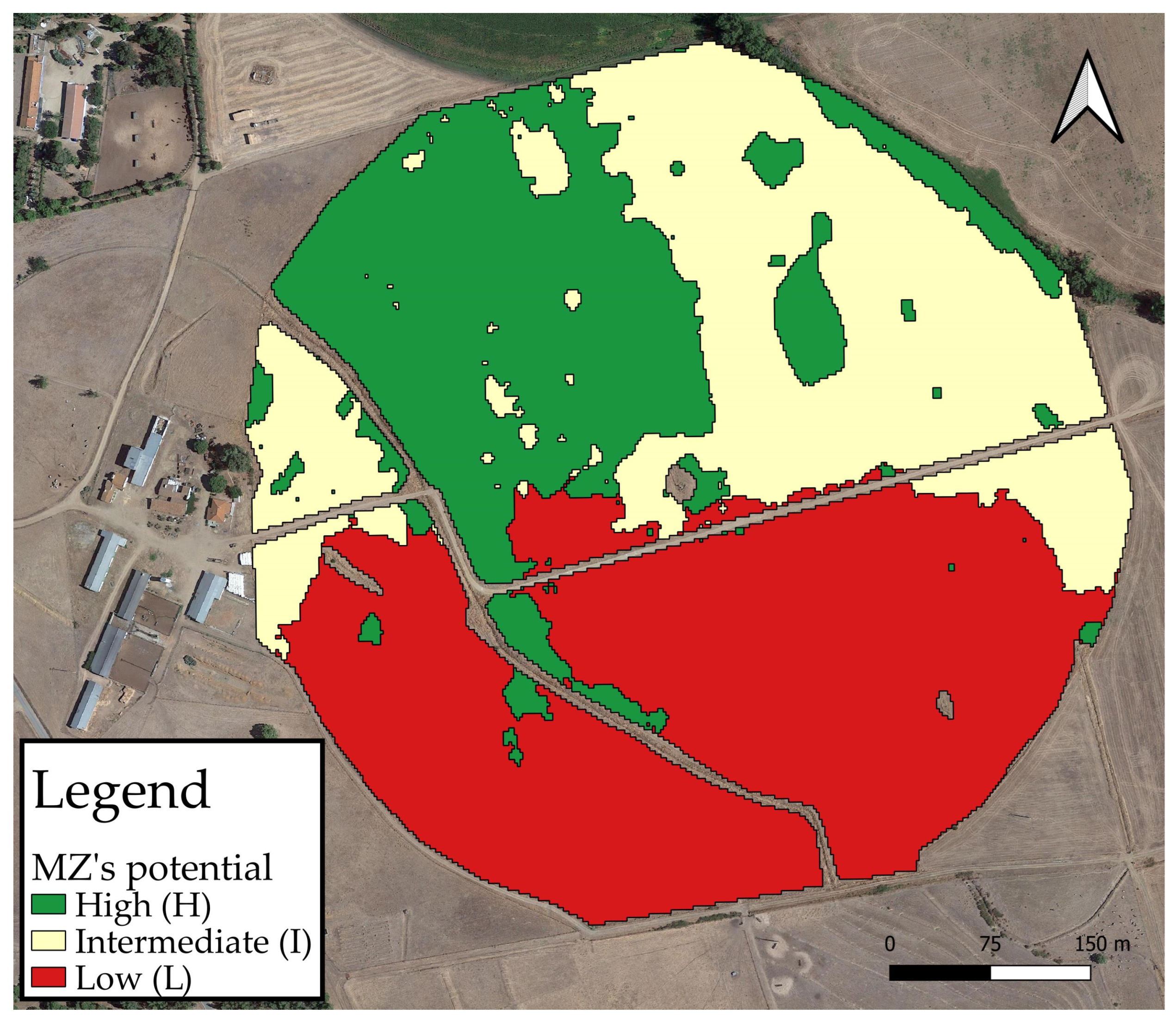
3.1.5. MZs’ Delineations Using Cluster Analysis
This research categorized the groups into three distinct levels: low potential (L), intermediate potential (I), and high potential (H). This decision was guided by practical considerations, as it was deemed crucial to define a limited number of homogeneous zones for ease of analysis [
37]. The final classified map (
Figure 7) was generated using an unsupervised classification technique on the sets of input layers that most influence the spatial variation of the soil. The ISO Cluster approach in ArcGIS was employed for classification purposes. This algorithm arranges the data in the input raster into a user-defined number of groups, generating signatures that are then utilized for classification through the “Maximum Likelihood Classifier” (MLC) function. In this study, the number of groups was set at three (low, intermediate, and high potential) to delineate only a few homogeneous zones, considering practical constraints.
Significant variations in soil properties were observed across the three MZs (
Table 15). MZ L had the highest sand value and lowest silt and clay values. The pH values increase from MZ L to MZ I and to MZ H, consecutively, such as occurs with Ca, Mg
exc, Na, and CEC values.
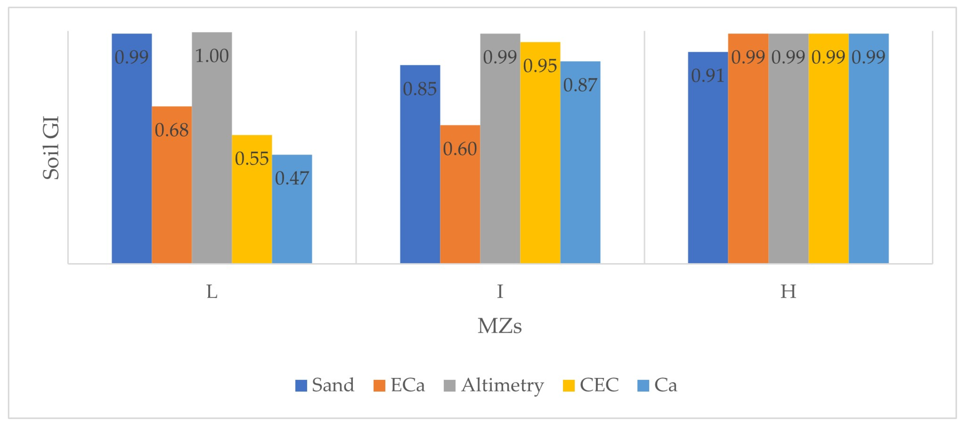
By the calculation of the GI of key soil parameters, it is evident that the lowest average value is found in zone L (0.74), the average value in zone I is 0.85, and the highest value occurs in zone H (0.94) (
Figure 8). This indicates that, except for sand, the highest values are present in the most fertile zones.
3.2. Crop Spatiotemporal Information
Meteorological Analysis and Influence on Crop Yield and Resource Utilization Efficiency
In
Figure 3, the ombrothermic diagram gathers the data for Tm and P from the 3 years of the trial and the CN. Related to temperature, only November of the second year and January of the first year were below the temperatures of the CN. All other records indicate temperatures above the normal. The third year had the highest temperatures in autumn and spring, while the second year recorded the highest values in the winter period. In the first year, the temperatures fluctuated considerably, to the extent that, for instance, January was the coldest month, yet February was the warmest. On average, the crop accumulated a total of 1380.7 GDD, with the lowest accumulation in the second year and the highest in the third year (
Table 16).
Regarding annual rainfall, the first year recorded the highest accumulated value (mm), followed by the third year (mm), and lastly, the second year (mm) (
Table 16).
In the first year, the months of November, February, and April had precipitation levels above the normal, while all other months were below average. For the second year, only March exceeded the average, with a value (87.7 mm) more than double the precipitation of the CN (39.6 mm). Precipitation levels during autumn and winter were notably low, to the extent that January and February almost had negligible values. In this second year of the trial (167.6 mm), approximately 72.6% of the precipitation occurred in the final phase of the crop cycle (L_mid) (
Table 16).
Lastly, in the third year, a total of 383.3 mm of precipitation occurred. However, in December alone, 253.3 mm of this precipitation fell, which accounts for 66% of the total. Of the remaining precipitation, 27% happened in November and January, indicating that 93% of the total precipitation occurred between November and January, followed by a dry spell until the end of the cycle. Thus, there was an extended summer period marked by a significant shortage of precipitation during the final phase of the crop cycle and a record of notably high temperatures.
There is also a correlation between the amount of precipitation in the final phase of the cycle and the applied N use efficiency (NUE). The first year recorded the highest precipitation in the final phase (82 mm) and the highest ratio of kg DM per unit of applied N (83.2 kg DM/N). This was followed by the second year with 49.3 mm of precipitation and an NUE of 67.1 kg DM/N. Lastly, the third year had the lowest precipitation (4.8 mm) and the lowest NUE (50.1 kg DM/N) (
Table 16).
3.3. Remote Sensing Data
By collecting Sentinel-2 images, it was possible to calculate NDVI, NDRE, and NDMI indices at harvest time. As shown in
Table 17, the index values decreased from year I to year II and year III.
By using the GI to validate the soil MZs, it is evident that the trend of soil properties significantly influences the behavior of crops and their vigor or stress across the plot. In
Figure 12, it is noticeable that zone L exhibits the lowest GI values, with an increase in these values for zone I and even further for zone H. Similar to NDVI, in NDRE, we observe a similar relationship and trend between the remotely sensed vegetative state and the trend of soil parameters in space. Among the three studied indices, NDMI shows GI values that most closely resemble the GI of soil properties. However, as previously discussed, in year I, the behaviors of zones H and L are reversed, with zone L displaying the highest GI value (0.99), not zone H (0.96).
4. Discussion
4.1. Soil MZs
Starting by analyzing the first data collected in the field to characterize the soil, it can be said that the CV of the ECa (27.47%) was higher than that of altimetry (1.58%) (
Table 8). The heightened CVs for the remaining soil properties highlighted significant spatial variability. Laboratory analysis of soil properties revealed that the soil of the study area tends to be sandy, and there is a tendency for a higher quantity of clay, compared to silt. The study area also tends to be slightly neutral. According to the soil nutrient classification of Portugal [
48], the mean of SOM content was low in the study area, while the mean of P and K were very high and high, respectively. The substantial values of CVs observed for the remaining soil properties indicated significant spatial variability. Therefore, implementing nutrient site-specific management was recommended to enhance soil productivity in the study area.
Most of the soil properties were significantly positive except those that are correlated with sand, which are negatively correlated. According to Shaddad et al. [
47], the lowest ME values indicated that the kriging predictions for soil properties closely aligned with the estimated values. Ideally, the MSSE value for each soil property should be one. However, if the MSSE value deviated from one but fell within the tolerance interval 1 ± 3 (2/N)1/2, where N represented the number of soil samples, the model was still considered accurate. According to the values presented in
Table 9 and
Table 12, the models chosen for all soil proprieties are in accordance with Shaddad et al. [
47]. The OK technique was employed to generate distribution maps, providing valuable information about nutrient content in the study area. This technique is widely used in these types of studies [
51], by allowing us knowing the spatial distribution of soil properties, and PCA may be applied. According to the results, it is possible to see the great importance of ECa, sand, altimetry, Ca, and CEC (
Table 14). Although they are all of great importance, it was necessary to use the Iso Cluster and MLC tools in this study, since the layers corresponding to each soil property joined a raster band, which needs to be classified in an unsupervised way. Only with this unsupervised classification—that is, not influenced by the human carrying out the analysis—was it possible to achieve the final MZs map shown in
Figure 7.
Analyzing the values of the soil proprieties within these three zones, is clear that all the MZs need an SOM input, because all of them have low classification, as suggested [
48]. The opposite occurs with the application of P, for which no major applications are necessary for any of the zones as they are all classified as having very high values. In the case of K, higher doses must be applied to MZ H and L, as they have a medium classification, while MZ I has a high classification, in which the application of P can be reduced. Furthermore, it was necessary to classify and order them according to their potential. The GI indicated that the area with the lowest potential is only superior in terms of sand and falls short of the other areas. This index ends up being a normalization of soil proprieties that compares them with the same parameters in the other two zones. The area with the greatest potential is only inferior in sand content. In this study, the altimetry does not show major differences between zones, since it is a field with very little relief (
Figure 5b) and with a very low CV that proves this, despite being one of the main properties at PCA.
This information could prove instrumental, offering recommendations for site-specific soil nutrient management. It aims to optimize output while simultaneously boosting income by minimizing input costs through the implementation of optimal management practices.
4.2. Multi-Year Weather Analysis
During the period of this study, the inter-annual variability of the Mediterranean climate became very clear. About the temperature, values suggest an advancement in crop growth and development due to the accumulation of GDD in the three years. As seen in
Table 16, the first year recorded a precipitation value more than double that of the CN. The second year was the only one that reported a value below (82 mm less), while the third year had a total precipitation above the CN. Notably, this precipitation was highly concentrated, occurring mainly during the intermediate phase of crop development, with a minimal amount of precipitation (4.8 mm) during the final stage. Thus, in addition to noticing an inter-annual variation, it was also noted that extreme phenomena occurred (such as the high concentration of precipitation in December of Year III), which are also characteristic of the Csa climate.
Regarding crop production, the first year was the most productive, followed by the second year, and finally, the third year. Therefore, there is not a direct correlation between the total precipitation and the quantity of production. However, there is a noticeable relationship between production quantity and precipitation during the final phase of the crop cycle. Given that this phase is critical for the growth and development of the crop, precipitation during this time is crucial as the crop’s demand is high and its response to precipitation episodes is highly favorable.
Precipitation at the end of the crop cycle also correlates well with the NUE. In the wettest year, the crop responded with a highest value of DM production per unit of applied N, whereas in the driest year, it responded with the lowest value of DM per unit of N (
Table 16).
In summary, some interesting relationships were found between the inter-annual variability of the Csa climate and the production and inputs’ use efficiency, namely N. Although some studies demonstrated the influence of intra-annual climate variability [
52], more future studies are still necessary to relate these influences, especially of Csa climate, and consider extreme phenomena that are increasingly regular with climate change, such as cases of high precipitation in a short period, or heat wave phenomena.
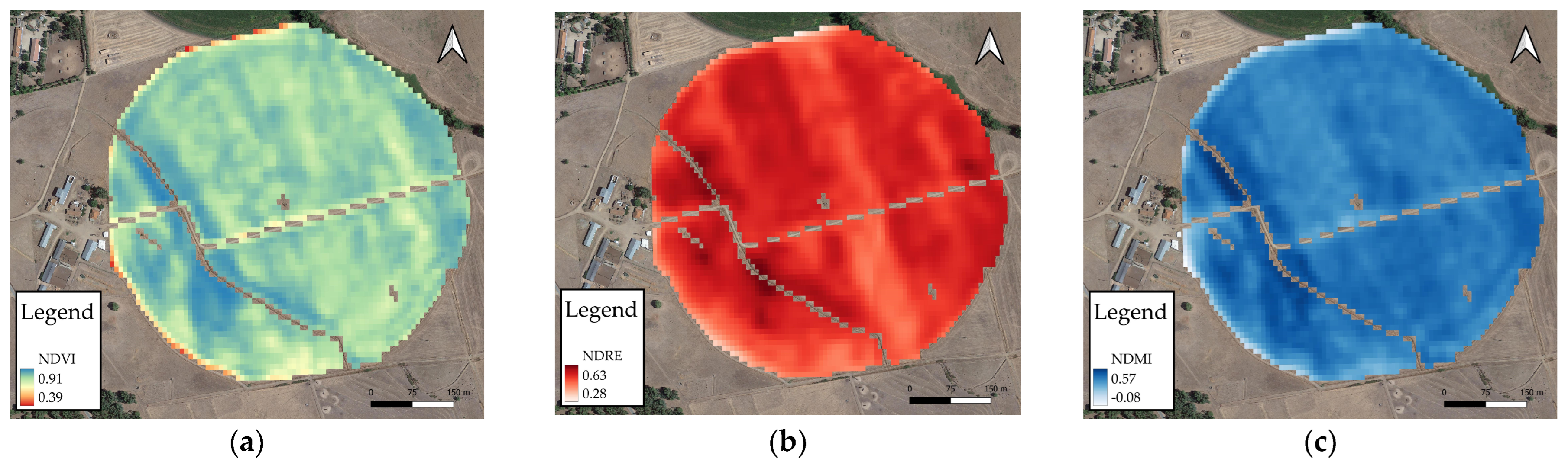
4.3. Zonal Analysis of Remotely Sensed Crop Vigor
The trend observed in the soil study persists in the VI over time. There is a correlation between precipitation in the final phase of the crop cycle, the production of DM, and the radiation emitted throughout the plots, which is used to calculate the vegetation indices. Generally, there is a decrease in the indices from zone H to zone I and then to zone L in each image. However, there is an exception in the NDMI map of year I, where the NDMI values are higher in zone L, followed by zone I, and lastly, lower values in zone H. As year I not only had the highest precipitation in the final phase but also throughout the entire cycle, the soil in zone H was waterlogged. Consequently, the crop behaved inversely, being more hydrologically comfortable in zone L and experiencing more stress in zone H. This result indicates that the analysis of IVs should not be carried out in a very generalized way, as it must also consider the climate, its characteristic irregularity, and therefore, the climate that is being felt in the year in question. Opposite of Year I is Year III, during which lower precipitation was recorded during the final stage of the cycle, underscoring how variations in soil properties are more distinct during years of higher stress. In years with more precipitation, the crop might be more homogeneous, or water might not be the limiting factor, requiring a deeper understanding of the relationship between crop vigor and other factors. These findings highlight an opportunity to address this issue in wetter years, indicating the need to explore potential enhancements in soil drainage conditions, particularly in zone H. However, in drier years, it also underscores the importance of considering the delineated MZs for studying varied irrigation prescriptions across these different areas.
It should be noted that, in general, all GIs of all IVs demonstrated the same trend in soil properties. This means that, with some exceptions already discussed, the high potential zone allows plants to have better vigor, while the lower potential zone contains plants with lower vigor. This tendency is accentuated in years in which plants feel greater stress.
Due to the tendency of NDVI to saturate in the final stages of the crop cycle or in situations of high biomass, it was decided to collect, process, and analyze the NDRE as well. In the case of this index that focuses on the near-infrared region, it notably highlights the radiation emitted by plants, especially in the advanced phases of the cycle, as in this case. The varied choice of IVs was the first mitigation measure used to address the possible uncertainties encountered in this study, due to its location and soil and climate conditions. Secondly, the choice of Sentinel-2 images was not only because they were freely available, but also due to the fact that these images were provided with the appropriate calibrations (including radiometric ones), thus eliminating possible biases introduced by sensor operators and due to the change in solar radiation at the time of image collection.
4.4. Contributions of this Study
Covering three years of weather data can provide a reasonable understanding of the typical variability within that specific timeframe, especially when comparing it to the CN. Although we agree that in scientific research, longer-term datasets are often preferred to understand climate variability, three years of data can still provide valuable information about short- to medium-term weather patterns and variability tendencies within that specific timeframe. Considering the type of crop and technical itinerary, although the methodological approach could be applied to other crops, the results of this study should be deemed valid specifically for rainfed annual crops.
The study goes forward to the Farm to Fork strategy [
53], considering the goals of promoting environmentally friendly practices and efficient use of resources, namely soil. With the proper delineation of MZs and the use of variable rate technologies (VRTs), farmers can avoid time and costs but most importantly are able to mitigate the agriculture impact, improve biodiversity, and promote more sustainable agricultural activities.
This study enhances theoretical and practical implications: theoretically related with the methods and algorithms used in delineating soil MZs, potentially refining existing methodologies or introducing new approaches; and practically related to cost savings for farmers by minimizing inputs where they are not needed, thereby reducing wastage and improving economic sustainability.
4.5. Uncertainties, Challenges, and Future Trends
In general, limitations and uncertainties that can affect the outcomes and conclusions of a study may be considered derived from sample size, data quality, methodological or temporal constraints, confounding variables or external validity. In our case study, although we intended to consider a farmer–field scale for the importance of the outcome to the farm sector, we are conscious that some confounding variables (e.g., soil parameters) may not be so controlled as in a smaller plot, which is the reason why we just can justify some of the correlations. Also, the external validity of the study is only possible considering similar crops—annual and cereal crops, and rainfed conditions. The entire process of delineating the MZs and validating them through remotely monitoring the crop VIs relied on digital technologies. However, quantifying this footprint was not the focus of this study, so it remains unquantified. It is a great interest that potentially this approach may have and should be considered in future research.
5. Conclusions
In this trial, georeferenced data obtained from a soil sensor for electrical conductivity, along with remote sensing, were utilized alongside in situ soil assessments to delineate MZs within a fodder crop. The results showed the great importance of ECa, sand, altimetry, Ca, and CEC proprieties of the soil. Based on these properties, three site-specific management areas could be selected where crop VIs took place.
The inter-annual variability of the Mediterranean climate became very clear in this study. There is a noticeable relationship between production quantity and precipitation during the final phase of the crop cycle. This precipitation also correlates well with the NUE. In summary, some interesting relationships were found between the inter-annual variability of the Csa climate and the DM production and inputs use efficiency, namely N.
Among the three studied indices, NDMI shows GI values that most closely resemble the GI of soil properties. It should be noted that, in general, all GIs of all IVs demonstrated the same trend in soil properties. This means that, with some exceptions already discussed, the high potential zone allows plants to have better vigor, while the lower potential zone contains plants with lower vigor. This tendency is accentuated in years in which plants feel greater stress. Critical opportunities for addressing environmental issues based on nuanced soil conditions and irrigation needs across different weather patterns were found, particularly emphasizing the enhancement of soil drainage in wetter years and tailored irrigation strategies for different zones in drier periods.
The results support the Farm to Fork strategy by advocating for environmentally friendly practices and efficient resource use, emphasizing soil management. Through precise delineation of MZs and the application of VRTs, farmers can reduce costs and time, while also addressing the environmental impact of agriculture, promoting biodiversity, and enhancing overall sustainability. This study improves soil management approaches theoretically by refining methods and algorithms and practically by helping farmers save costs through optimized input usage, reducing wastage, and enhancing economic sustainability.
The study of the influence of intra-annual variability on the remotely detected vigor of the crops, with influence on their clustering into homogeneous crop MZs, could be a trend of study in the future. As previously stated, the analysis and management of crops rely on data collected through digital technologies, known as the digitization footprint. This involves the demand for energy, storage, and processing resources to handle the generated data and information. Therefore, future research should consider calculating this digitization footprint as a point of interest.
Author Contributions
Conceptualization, L.A.C. and L.S.; methodology, L.A.C. and L.S.; software, L.S.; validation, L.A.C. and L.S.; formal analysis, L.A.C. and L.S.; investigation, L.A.C., L.S., C.V., L.L. and B.M.; resources, L.A.C., L.S., C.V., L.L. and B.M.; data curation, L.A.C.; writing—original draft preparation, L.A.C. and L.S.; writing—review and editing, L.A.C., L.S., C.V., L.L. and B.M.; visualization, L.A.C., L.S., C.V., L.L. and B.M.; supervision, L.A.C.; project administration, L.A.C. All authors have read and agreed to the published version of the manuscript.
Funding
This research received no external funding.
Institutional Review Board Statement
Not applicable.
Informed Consent Statement
Not applicable.
Data Availability Statement
Dataset available on request from the authors.
Conflicts of Interest
The authors declare no conflicts of interest.
References
- FAO. Status of the World’s Soil Resources (SWSR)–Main Report; Food and Agriculture Organization of the United Nations and Intergovernmental Technical Panel on Soils: Rome, Italy, 2015. [Google Scholar]
- Instituto Nacional de Estatística—Recenseamento Agrícola. Análise dos Principais Resultados: 2019; INE: Lisboa, Portugal, 2021; ISBN 978-989-25-0562-6.
- EUROSTAT. Agri-Environmental Indicator—Soil Erosion; EUROSTAT: Luxembourg, 2023. [Google Scholar]
- Carvalho, M.D.C.S.; Lourenço, E. Conservation agriculture—A Portuguese case study. J. Agron. Crop Sci. 2014, 200, 317–324. [Google Scholar] [CrossRef]
- Fiorentino, C.; Donvito, A.R.; D’Antonio, P.; Lopinto, S. Experimental Methodology for Prescription Maps of Variable Rate Nitrogenous Fertilizers on Cereal Crops. In Proceedings of the Innovative Biosystems Engineering for Sustainable Agriculture, Forestry and Food Production: International Mid-Term Conference 2019 of the Italian Association of Agricultural Engineering (AIIA), Matera, Italy, 12–13 September 2019. [Google Scholar]
- Bottega, E.L.; Marin, C.K.; de Oliveira, Z.B.; Lamb, C.d.C.; Amado, T.J.C. Soil Density Characterization in Management Zones Based on Apparent Soil Electrical Conductivity in Two Field Systems: Rainfeed and Center-Pivot Irrigation. Agriengineering 2023, 5, 460–472. [Google Scholar] [CrossRef]
- Brambilla, M.; Romano, E.; Toscano, P.; Cutini, M.; Biocca, M.; Ferré, C.; Comolli, R.; Bisaglia, C. From Conventional to Precision Fertilization: A Case Study on the Transition for a Small-Medium Farm. Agriengineering 2021, 3, 438–446. [Google Scholar] [CrossRef]
- Winkler, J.; Dvořák, J.; Hosa, J.; Barroso, P.M.; Vaverková, M.D. Impact of Conservation Tillage Technologies on the Biological Relevance of Weeds. Land 2022, 12, 121. [Google Scholar] [CrossRef]
- Hedley, C. The role of precision agriculture for improved nutrient management on farms. J. Sci. Food Agric. 2015, 95, 12–19. [Google Scholar] [CrossRef] [PubMed]
- Yuan, Y.; Shi, B.; Yost, R.; Liu, X.; Tian, Y.; Zhu, Y.; Cao, W.; Cao, Q. Optimization of Management Zone Delineation for Precision Crop Management in an Intensive Farming System. Plants 2022, 11, 2611. [Google Scholar] [CrossRef] [PubMed]
- Speranza, E.A.; Naime, J.d.M.; Vaz, C.M.P.; Santos, J.C.F.d.; Inamasu, R.Y.; Lopes, I.d.O.N.; Queirós, L.R.; Rabelo, L.M.; Jorge, L.A.d.C.; Chagas, S.d.; et al. Delineating Management Zones with Different Yield Potentials in Soybean–Corn and Soybean–Cotton Production Systems. AgriEngineering 2023, 5, 1481–1497. [Google Scholar] [CrossRef]
- King, J.A.; Dampney, P.M.R.; Lark, R.M.; Wheeler, H.C.; Bradley, R.I.; Mayr, T.R. Mapping Potential Crop Management Zones within Fields: Use of Yield-map Series and Patterns of Soil Physical Properties Identified by Electromagnetic Induction Sensing. Precis. Agric. 2005, 6, 167–181. [Google Scholar] [CrossRef]
- Moral, F.; Terrón, J.; da Silva, J.M. Delineation of management zones using mobile measurements of soil apparent electrical conductivity and multivariate geostatistical techniques. Soil Tillage Res. 2010, 106, 335–343. [Google Scholar] [CrossRef]
- Serrano, J.; Shahidian, S.; Silva, J.M.d. Spatial and Temporal Patterns of Apparent Electrical Conductivity: DUALEM vs. Veris Sensors for Monitoring Soil Properties. Sensors 2014, 14, 10024–10041. [Google Scholar] [CrossRef]
- Lawley, V.; Lewis, M.; Clarke, K.; Ostendorf, B. Site-based and remote sensing methods for monitoring indicators of vegetation condition: An Australian review. Ecol. Indic. 2016, 60, 1273–1283. [Google Scholar] [CrossRef]
- Loures, L.; Chamizo, A.; Ferreira, P.; Loures, A.; Castanho, R.; Panagopoulos, T. Assessing the Effectiveness of Precision Agriculture Management Systems in Mediterranean Small Farms. Sustainability 2020, 12, 3765. [Google Scholar] [CrossRef]
- Corwin, D.; Lesch, S. Characterizing soil spatial variability with apparent soil electrical conductivity: Part II. Case study. Comput. Electron. Agric. 2005, 46, 135–152. [Google Scholar] [CrossRef]
- Sudduth, K.A.; Kitchen, N.R.; Bollero, G.A.; Bullock, D.G.; Wiebold, W.J. Comparison of electromagnetic induction and direct sensing of soil electrical conductivity. Agron. J. 2003, 95, 472–482. [Google Scholar] [CrossRef]
- Bhandral, R.; Saggar, S.; Bolan, N.; Hedley, M. Transformation of nitrogen and nitrous oxide emission from grassland soils as affected by compaction. Soil Tillage Res. 2007, 94, 482–492. [Google Scholar] [CrossRef]
- Domsch, H.; Giebel, A. Estimation of Soil Textural Features from Soil Electrical Conductivity Recorded Using the EM38. Precis. Agric. 2004, 5, 389–409. [Google Scholar] [CrossRef]
- Serrano, J.; Shahidian, S.; Da Silva, J.M.; Moral, F.; Carvajal-Ramirez, F.; Carreira, E.; Pereira, A.; De Carvalho, M. Evaluation of the Effect of Dolomitic Lime Application on Pastures—Case Study in the Montado Mediterranean Ecosystem. Sustainability 2020, 12, 3758. [Google Scholar] [CrossRef]
- Rasmussen, J.; Ntakos, G.; Nielsen, J.; Svensgaard, J.; Poulsen, R.N.; Christensen, S. Are vegetation indices derived from consumer-grade cameras mounted on UAVs sufficiently reliable for assessing experimental plots? Eur. J. Agron. 2016, 74, 75–92. [Google Scholar] [CrossRef]
- Sankaran, S.; Maja, J.M.; Buchanon, S.; Ehsani, R. Huanglongbing (Citrus Greening) Detection Using Visible, Near Infrared and Thermal Imaging Techniques. Sensors 2013, 13, 2117–2130. [Google Scholar] [CrossRef]
- Köppen, W. Versuch einer Klassifikation der Klimate, vorzugsweise nach ihren Beziehungen zur Pflanzenwelt; (Schluss). Geogr. Z. 1900, 6, 657–679. [Google Scholar]
- Área Educativa IPMA. Available online: https://www.ipma.pt/pt/educativa/observar.tempo/index.jsp?page=ema.index.xml (accessed on 23 October 2023).
- Cardoso, J.C. A Classificação de Solos de Portugal; Boletim de Solos do S.R.O.A.: Lisboa, Portugal, 1974; pp. 14–46. [Google Scholar]
- ISO 11277:2020; Soil Quality—Determination of Particle Size Distribution in Mineral. Soil Material—Method by Sieving and Sedimentation. International Organization for Standardization: London, UK, 2020; p. 16.
- Walkley, A.; Black, L.A. An Examination of the Dgtjareff Method for Determining Soil Organic Matter, and a Proposed Modification of the Chromic Acid Titration Method. Soil Sci. 1934, 37, 29–38. [Google Scholar] [CrossRef]
- Egner, H.; Riehm, H.; Domingo, W.R. Investigations on the chemical soil analysis as a basis for assessing the soil nutrient status. II: Chemical extraction methods for phosphorus and potassium determination. K. Lantbrukshügskolans Ann. 1960, 26, 199–215. [Google Scholar]
- SR EN ISO 11260:2018; Soil Quality. Determining the Effective Cation Exchange Capacity and the Degree of Saturation in Bases. Institute for Standardization of Serbia, ISS: Belgrade, Serbia, 2018.
- Metwally, M.S.; Shaddad, S.M.; Liu, M.; Yao, R.-J.; Abdo, A.I.; Li, P.; Jiao, J.; Chen, X. Soil Properties Spatial Variability and Delineation of Site-Specific Management Zones Based on Soil Fertility Using Fuzzy Clustering in a Hilly Field in Jianyang, Sichuan, China. Sustainability 2019, 11, 7084. [Google Scholar] [CrossRef]
- Shashikumar, B.N.; Kumar, S.; George, K.J.; Singh, A.K. Soil variability mapping and delineation of site-specific management zones using fuzzy clustering analysis in a Mid-Himalayan Watershed, India. Environ. Dev. Sustain. 2023, 25, 8539–8559. [Google Scholar] [CrossRef]
- Goovaerts, P. Geostatistical tools for characterizing the spatial variability of microbiological and physico-chemical soil properties. Biol. Fertil. Soils 1998, 27, 315–334. [Google Scholar] [CrossRef]
- Meul, M.; Van Meirvenne, M. Kriging soil texture under different types of nonstationarity. Geoderma 2003, 112, 217–233. [Google Scholar] [CrossRef]
- Triantafilis, J.; Odeh, I.; McBratney, A. Five Geostatistical Models to Predict Soil Salinity from Electromagnetic Induction Data Across Irrigated Cotton. Soil Sci. Soc. Am. J. 2001, 65, 869–878. [Google Scholar] [CrossRef]
- Schepers, A.R.; Shanahan, J.F.; Liebig, M.A.; Schepers, J.S.; Johnson, S.H.; Luchiari, A., Jr. Appropriateness of management zones for characterizing spatial variability of soil properties and irrigated corn yields across years. Agron. J. 2004, 96, 195–203. [Google Scholar] [CrossRef]
- Serrano, J.; Shahidian, S.; Paixão, L.; da Silva, J.M.; Moral, F. Management Zones in Pastures Based on Soil Apparent Electrical Conductivity and Altitude: NDVI, Soil and Biomass Sampling Validation. Agronomy 2022, 12, 778. [Google Scholar] [CrossRef]
- Serrano, J.; Mau, V.; Rodrigues, R.; Paixão, L.; Shahidian, S.; da Silva, J.M.; Paniagua, L.L.; Moral, F.J. Definition and Validation of Vineyard Management Zones Based on Soil Apparent Electrical Conductivity and Altimetric Survey. Environments 2023, 10, 117. [Google Scholar] [CrossRef]
- Rain Detector DRD11A VAISALA. Available online: https://www.vaisala.com/en/products/weather-environmental-sensors/rain-detector-drd11a (accessed on 23 October 2023).
- Hutchinson, G.K. Aspects of accumulated heat patterns (growing degree-days) and pasture growth in Southland. In Proceedings of the New Zealand Grassland Association, Invercargill, New Zealand, 1 January 2000. [Google Scholar]
- Moreira, N. Agronomia das Forragens e Pastagens; Sector Editorial: Vila Real, Portugal, 2002. [Google Scholar]
- Iannucci, A.; Terribile, M.; Martiniello, P. Effects of temperature and photoperiod on flowering time of forage legumes in a Mediterranean environment. Field Crops Res. 2008, 106, 156–162. [Google Scholar] [CrossRef]
- McMaster, G.S.; Wilhelm, W.W. Growing degree-days: One equation, two interpretations. Agric. For. Meteorol. 1997, 87, 291–300. [Google Scholar] [CrossRef]
- Soares, D.J. Forragens Conservadas para Equinos em Contexto de Alterações Climáticas. Master Thesis, Superior Institute of Agronomy, University of Lisbon, Lisbon, Portugal, 2019. [Google Scholar]
- Copernicus Browser. Available online: https://dataspace.copernicus.eu/browser/ (accessed on 11 November 2023).
- EOS Data Analytics. Available online: https://eos.com/make-an-analysis/ (accessed on 13 November 2023).
- Shaddad, S.; Buttafuoco, G.; Elrys, A.; Castrignanò, A. Site-specific management of salt affected soils: A case study from Egypt. Sci. Total. Environ. 2019, 688, 153–161. [Google Scholar] [CrossRef] [PubMed]
- INIAP—Laboratório Químico Agrícola Rebelo da Silva. Manual de Fertilização das Culturas, 2nd ed.; INIAP: Lisboa, Portugal, 2005.
- Jakobsen, B.H. Soil Spatial Variability. In Proceedings of the a Workshop of the ISSS and the SSSA, Las Vegas, NV, USA, 30 November–1 December 1984; International Society of Soil Science: Madison, WI, USA, 1984. [Google Scholar]
- Sharma, S. Applied Multivariate Techniques; Wiley: New York, NY, USA, 1996. [Google Scholar]
- Rodrigues, H.; Ceddia, M.B.; Vasques, G.M.; Mulder, V.L.; Heuvelink, G.B.M.; Oliveira, R.P.; Brandão, Z.N.; Morais, J.P.S.; Neves, M.L.; Tavares, S.R.L. Remote Sensing and Kriging with External Drift to Improve Sparse Proximal Soil Sensing Data and Define Management Zones in Precision Agriculture. Agriengineering 2023, 5, 2326–2348. [Google Scholar] [CrossRef]
- Bahat, I.; Netzer, Y.; Grünzweig, J.M.; Alchanatis, V.; Peeters, A.; Goldshtein, E.; Ohana-Levi, N.; Ben-Gal, A.; Cohen, Y. In-Season Interactions between Vine Vigor, Water Status and Wine Quality in Terrain-Based Management-Zones in a ‘Cabernet Sauvignon’ Vineyard. Remote Sens. 2021, 13, 1636. [Google Scholar] [CrossRef]
- European Commission. European Commission Communication COM/2020/381. Communication from the Commission to the European Parliament, the Council, the European Economic and Social Committee and the Committee of the Regions: A Farm to Fork Strategy for a Fair, Healthy and Environmentally-Friendly food System. Available online: https://eur-lex.europa.eu/resource.html?uri=cellar:ea0f9f73-9ab2-11ea-9d2d-01aa75ed71a1.0001.02/DOC_1&format=PDF (accessed on 7 November 2023).
Figure 1.
Identification and delimitation of the experimental field and useless areas such as a drainage canal and a pathway.
Figure 1.
Identification and delimitation of the experimental field and useless areas such as a drainage canal and a pathway.
Figure 2.
(a) Schematic detail of the ECa paths transects across the field; (b) bullets represent the location of the soil sampling evaluation.
Figure 2.
(a) Schematic detail of the ECa paths transects across the field; (b) bullets represent the location of the soil sampling evaluation.
Figure 3.
The ombrothermic diagram that gathers the data for Tm and P from CN and the 3 years of the trial.
Figure 3.
The ombrothermic diagram that gathers the data for Tm and P from CN and the 3 years of the trial.
Figure 4.
(a) ECa semivariogram; (b) altimetry semivariogram.
Figure 4.
(a) ECa semivariogram; (b) altimetry semivariogram.
Figure 5.
(a) ECa map; (b) altimetry map.
Figure 5.
(a) ECa map; (b) altimetry map.
Figure 6.
Maps of the first four PCs.
Figure 6.
Maps of the first four PCs.
Figure 7.
Soil MZs of the study area.
Figure 7.
Soil MZs of the study area.
Figure 8.
GI of five soil parameters most influenced by PCA, for each homogeneous MZ in the experimental field. GI—Global Index; ECa—Soil apparent Electrical Conductivity; CEC—cation exchange capacity; Ca—exchangeable calcium.
Figure 8.
GI of five soil parameters most influenced by PCA, for each homogeneous MZ in the experimental field. GI—Global Index; ECa—Soil apparent Electrical Conductivity; CEC—cation exchange capacity; Ca—exchangeable calcium.
Figure 9.
Year I: (a) NDVI; (b) NDRE; (c) NDMI.
Figure 9.
Year I: (a) NDVI; (b) NDRE; (c) NDMI.
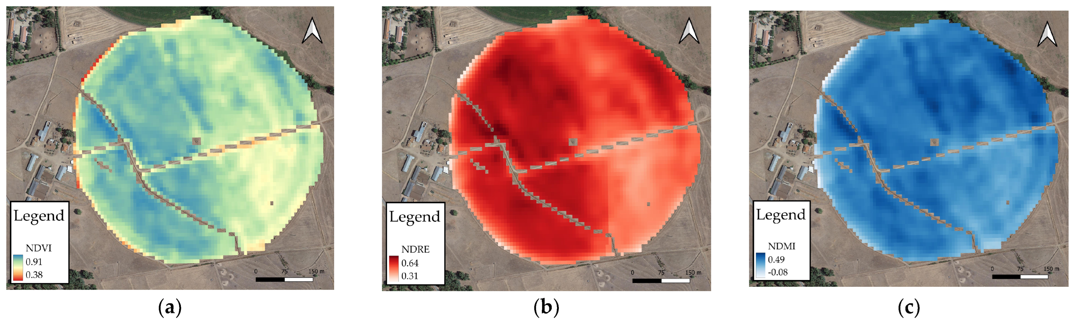
Figure 10.
Year II: (a) NDVI; (b) NDRE; (c) NDMI.
Figure 10.
Year II: (a) NDVI; (b) NDRE; (c) NDMI.
Figure 11.
Year III: (a) NDVI; (b) NDRE; (c) NDMI.
Figure 11.
Year III: (a) NDVI; (b) NDRE; (c) NDMI.
Figure 12.
GI of soil parameters and NDVI by year, for each homogeneous MZ in the experimental field. MZs—management zones; NDVI—Normalized Difference Vegetation Index; NDRE—Normalized Difference Red-Edge Index; NDMI—Normalized Difference Moisture Index.
Figure 12.
GI of soil parameters and NDVI by year, for each homogeneous MZ in the experimental field. MZs—management zones; NDVI—Normalized Difference Vegetation Index; NDRE—Normalized Difference Red-Edge Index; NDMI—Normalized Difference Moisture Index.
Table 1.
CN (1971–2000) including Tm and P values of Elvas [
25].
Table 1.
CN (1971–2000) including Tm and P values of Elvas [
25].
| Month | Tm (°C) | P (mm) |
|---|
| October | 17.4 | 58.6 |
| November | 12.5 | 75.1 |
| December | 9.7 | 92.6 |
| January | 8.6 | 63.1 |
| February | 10.2 | 54.6 |
| March | 12.3 | 39.6 |
| April | 14.1 | 51.2 |
| May | 17.3 | 44.0 |
| Total | 12.8 | 478.8 |
Table 2.
Composition of the mixture fodder crop sowed.
Table 2.
Composition of the mixture fodder crop sowed.
| Species | Cultivar | Mix Composition (%) |
|---|
| Lolium multiflorum L. | Hellen | 67 |
| Trifolium vesiculosum | Comm | 10 |
| Trifolium resupinatum | Lightning | 17 |
| Trifolium michelianum | Balansa Paradana | 6 |
Table 3.
Seed and fertilizer applied during each year of the study and their average.
Table 3.
Seed and fertilizer applied during each year of the study and their average.
| Year | Seeds (No./m2) | N (Units) | P (Units) | K (Units) |
|---|
| (I) | 1200 | 81.7 | 17.5 | 55.0 |
| (II) | 1200 | 83.9 | 23.0 | 46.0 |
| (III) | 1200 | 68.1 | 16.1 | 13.8 |
| Average | 1200 | 77.9 | 18.9 | 38.3 |
Table 4.
Dates of the agricultural operations conducted over the three years of the trial.
Table 4.
Dates of the agricultural operations conducted over the three years of the trial.
| Operation | Task | (I) | (II) | (III) |
|---|
| Phytosanitary treatment | Pre-emergence herbicide | 23 October | 15 October | 26 October |
| Fertilization | Basal dressing | 27 October | 17 November | 28 October |
| Sowing | Direct seeding | 30 October | 18 November | 7 November |
| Harvest | 1st cut | 15 January | 10 February | - |
| Fertilization | 1st Topdressing N | 24 February | 11 February | 30 January |
| Fertilization | 2nd Topdressing N | 24 March | - | - |
| Harvest | 2nd cut | 2 May | 5 May | 6 May |
Table 5.
Reference values of GDD for 1 cut per year and 2 cuts per year [
44].
Table 5.
Reference values of GDD for 1 cut per year and 2 cuts per year [
44].
| | 1 Cut | 2 Cuts |
|---|
| Seeding day/month | 15 October | 15 October |
| Tbase (°C) | 5 | 5 |
| | | 1st | 2nd |
| L_ini (GDD) | 308.3 | 285.8 | 148.8 |
| L_dev (GDD) | 774.9 | 633.2 | 282.9 |
| L_mid (GDD) | 402.4 | 282.5 | |
| Total of GDD | 1485.6 | 1633.2 |
| Total of days | 210 | 222 (2 cuts) |
Table 6.
Summary of the image capture moments.
Table 6.
Summary of the image capture moments.
| Crop Growth Stage | Task | (I) | (II) | (III) |
|---|
| Feekes 10.0–10.5 (Boot Stage-Heading) | Remote sensing data | 1 May 2021 | 1 May 2022 | 1 May 2023 |
| Final harvest | 2 May 2021 | 5 May 2022 | 6 May 2023 |
Table 7.
VIs computed to crop monitoring.
Table 7.
VIs computed to crop monitoring.
| VI | Band | Spatial Resolution (m) | Central Wavelength (nm) | Bandwidth (nm) | Formula |
|---|
| NDVI | B04 | 10 | 664.6 | 30 | (B08 − B04)/(B08 + B04) |
| B08 | 10 | 832.8 | 105 |
| NDRE | B05 | 20 | 704.1 | 14 | (B09 − B05)/(B09 + B05) |
| B09 | 60 | 945.1 | 19 |
| NDMI | B08 | 10 | 832.8 | 105 | (B08 − B11)/(B08 + B11) |
| B11 | 20 | 1613.7 | 90 |
Table 8.
Descriptive statistics for the ECa and altimetry soil properties.
Table 8.
Descriptive statistics for the ECa and altimetry soil properties.
| | No. of Samples | Mean ± SD | Range | CV |
|---|
| ECa | 15,091 | 27.33 ± 7.51 | 0.27–62.62 | 27.47 |
| Altimetry | 15,091 | 180.43 ± 2.86 | 173.15–190.50 | 1.58 |
Table 9.
The study area ECa and altimetry properties’ semi-variogram parameters.
Table 9.
The study area ECa and altimetry properties’ semi-variogram parameters.
| Soil Propriety | Model | Nugget | Partial Sill | Range (m) | ME | MSSE | ASE |
|---|
| ECa | circular | 0.027 | 3.300 | 0.001 | −0.002 | 0.886 | 0.309 |
| Altimetry | spherical | 0.450 | 35.527 | 0.000 | 0.000 | 0.931 | 1.489 |
Table 10.
Descriptive statistics for the studied soil properties.
Table 10.
Descriptive statistics for the studied soil properties.
| Soil Propriety | Mean ± SD | Range | CV |
|---|
| Sand (%) | 70.6 ± 5.7 | 61.2–79.1 | 8.1 |
| Silt (%) | 12.8 ± 2.1 | 8.6–16.9 | 16.8 |
| Clay (%) | 16.6 ± 4.4 | 8.5–23.9 | 26.6 |
| pH | 6.8 ± 0.4 | 5.8–7.6 | 6.6 |
| SOM (g kg−1) | 1.2 ± 0.3 | 0.8–1.8 | 21.1 |
| P (mg P2O5 kg−1) | 218.6 ± 96.0 | 103.1–427.4 | 43.9 |
| K (mg K2O kg−1) | 109.0 ± 78.1 | 43.2–427.2 | 71.6 |
| Mg (mg Mg kg−1) | 226.9 ± 91.8 | 108.8–396.7 | 40.5 |
| Ca (cmol (+) kg−1) | 5.3 ± 2.1 | 2.2–9.3 | 40.2 |
| Mgexc (cmol (+) kg−1) | 2.0 ± 0.7 | 0.9–3.5 | 37.1 |
| Kexc (cmol (+) kg−1) | 0.2 ± 0.2 | 0.0–0.9 | 90.0 |
| Na (cmol (+) kg−1) | 0.1 ± 0.1 | 0.1–0.2 | 36.0 |
| CEC (cmol (+) kg−1) | 7.9 ± 2.7 | 4.1–13.9 | 33.6 |
| Altimetry (m) | 180.1 ± 2.1 | 175.3–182.5 | 1.2 |
| ECa | 28.3 ± 7.7 | 18.1–48.1 | 27.2 |
Table 11.
Correlation coefficient values show the relationship among the study area soil properties.
Table 11.
Correlation coefficient values show the relationship among the study area soil properties.
| | Sand | Silt | Clay | pH | SOM | P | K | Mg | Ca | Mgexc | Kexc | Na | CEC | * Alt | ECa |
|---|
| Sand | 1.000 | | | | | | | | | | | | | | |
| Silt | −0.719 | 1.000 | | | | | | | | | | | | | |
| Clay | −0.941 | 0.443 | 1.000 | | | | | | | | | | | | |
| pH | −0.372 | 0.439 | 0.268 | 1.000 | | | | | | | | | | | |
| SOM | 0.118 | −0.074 | −0.116 | −0.242 | 1.000 | | | | | | | | | | |
| P | −0.100 | 0.368 | −0.050 | 0.163 | 0.325 | 1.000 | | | | | | | | | |
| K | −0.293 | 0.132 | 0.313 | −0.057 | −0.184 | 0.104 | 1.000 | | | | | | | | |
| Mg | −0.825 | 0.548 | 0.800 | 0.520 | −0.066 | 0.083 | 0.072 | 1.000 | | | | | | | |
| Ca | −0.738 | 0.516 | 0.703 | 0.708 | −0.085 | 0.069 | −0.005 | 0.852 | 1.000 | | | | | | |
| Mgexc | −0.800 | 0.571 | 0.756 | 0.605 | −0.018 | 0.061 | 0.016 | 0.933 | 0.912 | 1.000 | | | | | |
| Kexc | −0.075 | −0.029 | 0.111 | −0.179 | −0.069 | −0.018 | 0.606 | −0.121 | −0.176 | −0.157 | 1.000 | | | | |
| Na | −0.776 | 0.497 | 0.762 | 0.432 | −0.007 | 0.188 | 0.367 | 0.802 | 0.765 | 0.736 | 0.105 | 1.000 | | | |
| CEC | −0.795 | 0.534 | 0.767 | 0.629 | −0.054 | 0.069 | 0.061 | 0.891 | 0.986 | 0.947 | −0.083 | 0.801 | 1.000 | | |
| Alt * | −0.230 | 0.202 | 0.199 | 0.276 | −0.133 | −0.335 | −0.298 | 0.142 | 0.255 | 0.215 | −0.091 | −0.117 | 0.225 | 1.000 | |
| ECa | 0.099 | 0.170 | −0.210 | 0.614 | 0.007 | 0.026 | −0.285 | 0.117 | 0.297 | 0.233 | −0.307 | 0.015 | 0.209 | 0.215 | 1.000 |
Table 12.
The study area soil properties’ semi-variogram parameters.
Table 12.
The study area soil properties’ semi-variogram parameters.
| Model | Nugget | Partial Sill | Sill | Nugget/Sill | SDC | Range (m) | ME | MSSE | ASE |
|---|
| Sand | circular | 0.000 | 23.170 | 23.170 | 0.0000 | Strong | 0.002 | −0.009 | 0.961 | 3.623 |
| Silt | circular | 4.087 | 0.000 | 4.087 | 1.0000 | Weak | 0.002 | −0.034 | 0.938 | 2.141 |
| Clay | exponential | 0.000 | 6.618 | 6.618 | 0.0000 | Strong | 0.001 | 0.010 | 0.865 | 2.599 |
| pH | gaussian | 0.083 | 0.179 | 0.262 | 0.3168 | Moderate | 0.005 | 0.011 | 1.038 | 0.337 |
| SOM | stable | 0.020 | 0.047 | 0.067 | 0.2985 | Strong | 0.003 | 0.009 | 0.968 | 0.262 |
| Ca | exponential | 1.780 | 0.000 | 1.780 | 1.0000 | Weak | 0.001 | −0.044 | 0.904 | 1.441 |
| Mgexc | circular | 0.211 | 0.000 | 0.211 | 1.0000 | Weak | 0.001 | −0.027 | 0.963 | 0.498 |
| Kexc | gaussian | 0.004 | 0.029 | 0.033 | 0.1212 | Strong | 0.001 | −0.003 | 1.265 | 0.168 |
| Na | circular | 0.001 | 0.002 | 0.003 | 0.3333 | Moderate | 0.003 | −0.024 | 0.858 | 0.042 |
| CEC | exponential | 2.838 | 0.000 | 2.838 | 1.0000 | Weak | 0.001 | −0.049 | 0.901 | 1.819 |
Table 13.
PCA of soil properties.
Table 13.
PCA of soil properties.
| PC Layer | Eigen Value | Component Loading (%) | Accumulative
Loading (%) |
|---|
| 1 | 30.94 | 51.06 | 51.06 |
| 2 | 22.28 | 36.77 | 87.82 |
| 3 | 5.51 | 9.09 | 96.91 |
| 4 | 1.47 | 2.43 | 99.34 |
| 5 | 0.29 | 0.47 | 99.81 |
| 6 | 0.08 | 0.13 | 99.94 |
| 7 | 0.02 | 0.03 | 99.97 |
| 8 | 0.01 | 0.02 | 99.99 |
| 9 | 0.01 | 0.01 | 100.00 |
| 10 | 0.00 | 0.00 | 100.00 |
| 11 | 0.00 | 0.00 | 100.00 |
| 12 | 0.00 | 0.00 | 100.00 |
Table 14.
Loading coefficient for the first four PCs.
Table 14.
Loading coefficient for the first four PCs.
| | Sand | Silt | Clay | pH | SOM | Ca | Mgexc | Kexc | Na | CEC | Alt | ECa |
|---|
| PC1 | 0.546 | −0.096 | −0.410 | −0.024 | 0.006 | −0.196 | −0.072 | 0.001 | −0.004 | −0.254 | 0.015 | −0.645 |
| PC2 | 0.475 | −0.049 | −0.384 | −0.001 | 0.008 | −0.113 | −0.049 | −0.006 | −0.004 | −0.170 | 0.036 | 0.761 |
| PC3 | 0.054 | 0.097 | −0.130 | 0.074 | 0.014 | 0.236 | 0.078 | −0.023 | −0.002 | 0.242 | 0.918 | −0.043 |
| PC4 | −0.213 | −0.164 | 0.334 | −0.089 | −0.016 | −0.534 | −0.132 | 0.033 | −0.007 | −0.589 | 0.392 | 0.053 |
Table 15.
The average values of soil properties within the three MZs.
Table 15.
The average values of soil properties within the three MZs.
| | Sand | Silt | Clay | pH | SOM | P | K | Ca | Mgexc | Kexc | Na | CEC | Alt | ECa |
|---|
| H | 69.46 | 13.33 | 17.20 | 7.12 | 1.22 | 224.29 | 95.88 | 6.65 | 2.38 | 0.18 | 0.16 | 9.43 | 180.76 | 35.81 |
| I | 65.12 | 13.77 | 21.10 | 6.64 | 1.17 | 205.65 | 170.20 | 5.79 | 2.32 | 0.33 | 0.18 | 8.99 | 178.98 | 21.36 |
| L | 76.26 | 11.31 | 12.43 | 6.39 | 1.33 | 221.31 | 79.50 | 3.13 | 1.24 | 0.24 | 0.09 | 5.23 | 180.07 | 24.25 |
Table 16.
Summary of accumulated meteorological, production, and efficiency use of N data, by year.
Table 16.
Summary of accumulated meteorological, production, and efficiency use of N data, by year.
| | CN | I | II | III |
|---|
| Number of days | 210 | 185 | 169 | 184 |
| GDD total | 1485.6 | 1446.7 | 1150.8 | 1546.8 |
| P total | 259.2 | 536.4 | 171.1 | 383.3 |
| L_ini | 75.1 | 128.3 | 7.7 | 93.9 |
| L_dev | 165.9 | 325.1 | 114.1 | 284.6 |
| L_mid | 18.2 | 83.0 | 49.3 | 4.8 |
| FM (kg/ha) | - | 17,732.4 | 8366.3 | 4013.7 |
| DM (kg/ha) | - | 6801.3 | 5630.8 | 3411.6 |
| kg DM/N | - | 83.2 | 67.1 | 50.1 |
Table 17.
Mean values of remote sensing IVs in each MZ.
Table 17.
Mean values of remote sensing IVs in each MZ.
| | | NDVI | NDRE | NDMI |
|---|
| | | I | II | III | I | II | III | I | II | III |
|---|
| MZ | H | 0.81 | 0.81 | 0.68 | 0.54 | 0.57 | 0.42 | 0.39 | 0.35 | 0.24 |
| I | 0.79 | 0.76 | 0.64 | 0.53 | 0.52 | 0.40 | 0.40 | 0.34 | 0.21 |
| L | 0.79 | 0.77 | 0.61 | 0.52 | 0.52 | 0.40 | 0.41 | 0.30 | 0.15 |
| Mean | 0.80 | 0.78 | 0.64 | 0.53 | 0.54 | 0.41 | 0.40 | 0.33 | 0.20 |
| Disclaimer/Publisher’s Note: The statements, opinions and data contained in all publications are solely those of the individual author(s) and contributor(s) and not of MDPI and/or the editor(s). MDPI and/or the editor(s) disclaim responsibility for any injury to people or property resulting from any ideas, methods, instructions or products referred to in the content. |
© 2024 by the authors. Licensee MDPI, Basel, Switzerland. This article is an open access article distributed under the terms and conditions of the Creative Commons Attribution (CC BY) license (https://creativecommons.org/licenses/by/4.0/).


 ,
, 


