IOT-Enabled Model for Weed Seedling Classification: An Application for Smart Agriculture

Abstract

Smart agriculture is a concept that refers to a revolution in the agriculture industry that promotes the monitoring of activities necessary to transform agricultural methods to ensure food security in an ever-changing environment. These days, the role of technology is increasing rapidly in every sector. Smart agriculture is one of these sectors, where technology is playing a significant role. The key aim of smart farming is to use the technologies to increase the quality and quantity of agricultural products. IOT and digital image processing are two commonly utilized technologies, which have a wide range of applications in agriculture. IOT is an abbreviation for the Internet of things, i.e., devices to execute different functions. Image processing offers various types of imaging sensors and processing that could lead to numerous kinds of IOT-ready applications. In this work, an integrated application of IOT and digital image processing for weed plant detection is explored using the Weed-ConvNet model to provide a detailed architecture of these technologies in the agriculture domain. Additionally, the regularized Weed-ConvNet is designed for classification with grayscale and color segmented weed images. The accuracy of the Weed-ConvNet model with color segmented weed images is 0.978, which is better than 0.942 of the Weed-ConvNet model with grayscale segmented weed images.

1. Introduction

These days, the world has more IOT-connected devices than humans. The Internet of things (IOT) is a theory which defines the notion of interrelated computing nodes, devices, or things being linked to the Internet and being able to link themselves to other computing devices [1]. It mainly comprises networks, sensor equipment, and wireless communications. The Internet of things includes electronic appliances, linked security systems, vehicles, thermostats, vending machines, ATMs, speaker systems, buildings, alarm clocks, and a wide range of other applications. The Internet of things is used to advance intelligence by offering a high level of interaction between the environment and humans. It improves reliability, flexibility, and proficiency by focusing on time saving, cost reduction, and resource usage [2]

Visual information is the most significant sort of information that can be observed, extracted, and understood by humans. Visual information processing consists of almost one third of the cortical area of the human brain. Image processing is an area that performs some processes on an acquired image generally to enhance the quality of the image or to analyze it to obtain some information [3]. Currently, image processing and analysis is among the speedily rising applied technologies. It has diverse uses such as medical image processing, remote sensing, machine vision, robotics, video processing, surveillances, self-driving cars, gesture recognitions, and many more [4].

Smart agriculture is a mechanism for agriculture farm supervision that practices information technology to ensure that the crops and soil obtain precisely what is essential for the finest productivity. The aim of smart agriculture is to ensure productivity, sustainability, and safety [5]. Smart agriculture heavily depends on specific equipment and information technology. The smart agriculture methods include real-time monitoring of crops, soil, and environment. During the last decades, smart agriculture was restricted to operations that could assist in information technology infrastructure. Additionally, related computational resources needed to be fully implemented and benefited from the profits of precision agriculture. Nowadays, mobile computing applications, smart sensors, cloud computing, and drones promote smart agriculture as feasible for farming at any scale [6,7].

The numerous roles of Internet of things technologies in smart agriculture are crop observation, water management, soil management, and pesticide control. The enhanced responsiveness of operations is one of the advantages of employing IOT in agriculture. Farmers can swiftly react to any substantial change in air, weather, humidity, quality, or the condition of each crop or soil in the field using real-time surveillance and forecast systems. Moreover, the Internet of things, with its real-time, precise, and joint characteristics can offer great modifications to the agricultural supply chain management and deliver a critical technology for forming an even flow of agricultural logistics [8,9]. Systems, drones, remotes, remote sensors, and computer imaging, combined with IOT are utilized in smart agriculture to supervise surveys, crops, and map fields, as well as deliver data to farmers for rational farm management plans to save both money and time.

There are several uses of digital image processing in smart farming. Digital Image processing has been demonstrated to be an effective mechanism for processing analysis in multiple applications of smart agriculture and farming [10]. Various kinds of imaging methods such as photometric feature-based imaging, fluorescence imaging, thermal imaging, and hyper-spectral imaging have considerably contributed to the last decades [11]. The accessibility of wireless communication networks along with image processing methods can transform the condition of receiving effective expert guidance within a short period and at reasonable price. It has an extensive range of uses such as crop management, fruit grading, plant health monitoring, nutrient deficiency recognition, weed recognition and plant height/size analysis. The image processing-based analysis of the parameters has been demonstrated to be precise and less time consuming compared with conventional approaches [12].

Image processing and Internet of things have so far been used for several applications individually. Various separate applications of these tools are available in agriculture and have attained degrees of success; however, very few applications are offered with the integration of both these technologies. By integration of digital image processing and IOT, better results can be obtained in the smart agriculture domain [13,14]. Some studies such as “Implementation of IoT and Image processing in smart agriculture” have offered the integration of these technologies. This work has offered a method to integrate IOT and digital image processing to determine environmental factors or man-made factors such as pesticides and fertilizers that are explicitly obstructing the progress of a plant [15]. The rest of the work is distributed into Section 2, Section 3 and Section 4. Section 2 provides the details of the proposed framework for an IOT-enabled framework for smart agriculture, which includes an example of weed seedling classification. Section 3 discusses the experiment and results and Section 4 presents the conclusions. This work offers the following contributions:

• An IOT-enabled framework for smart agriculture;
• Design of a well regularized CNN framework for weed seedling classification;
• Analysis of the performance of weed seedling classification based on grayscale and color channel information.

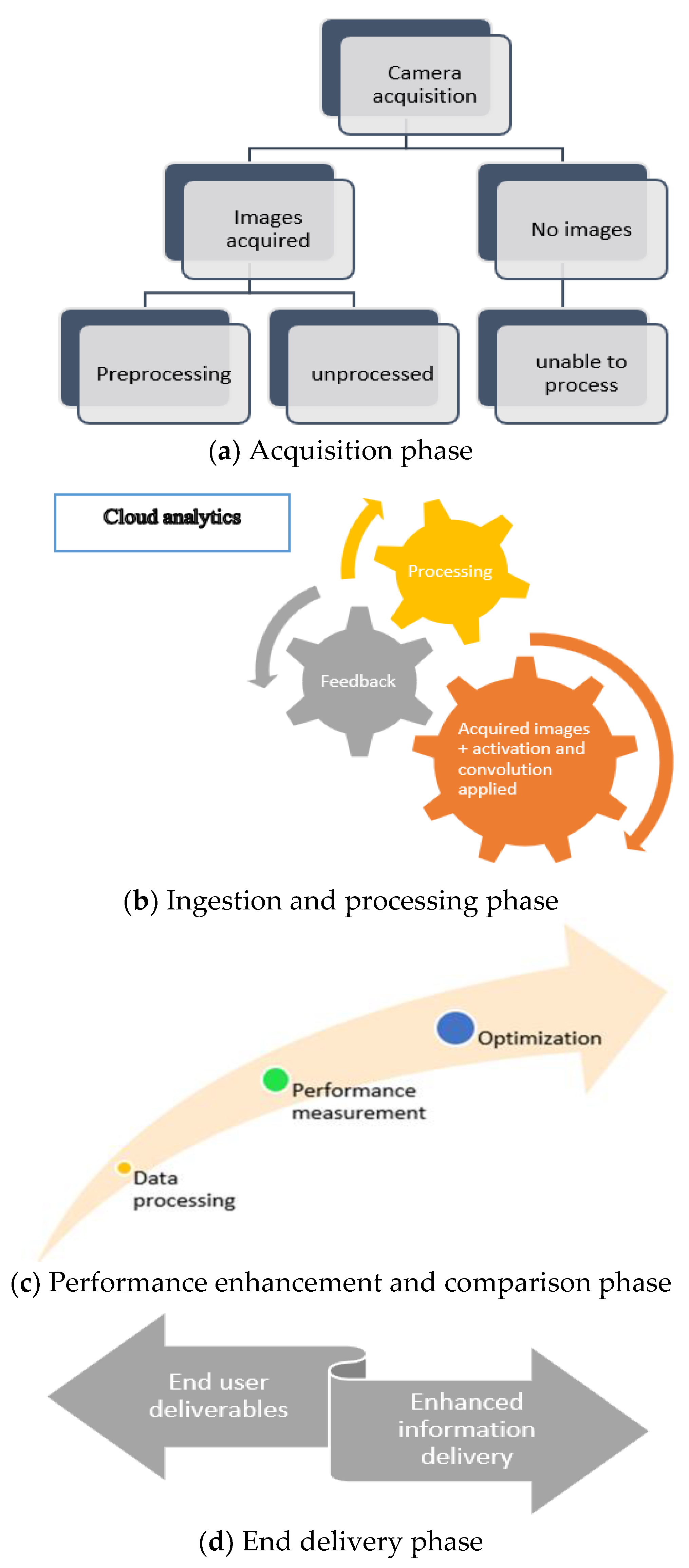
2. Methods

A weed plant is undesirable and in most situations it is “a plant in the wrong place”. Weed control is important in smart agriculture. Weed plant control is the botanical section of pest control that aims to end weeds, particularly harmful weeds, from contending with wanted flora and fauna comprising domesticated plants and livestock, and in natural situations stopping non-native species that compete with native species. Approaches for weed control comprise chemical attack with herbicides, hand cultivation with hoes, powered cultivation with cultivators, stifling with mulch or soil solarization, lethal wilting with extraordinary heat, or burning [16]. However, detection of the weed plant is necessary for weed control by herbicides [17]. This section gives an overall design for an example of a setup for weed plant classification application in the smart agriculture domain. The IOT and image analytics on the cloud model for weed plant seedling detection is presented in Figure 1. In this model, the IOT device is used to capture and transfer the image of the weed plant to the cloud using a wireless network. The image analytics is performed on the cloud and the message is communicated to the farmer.

Figure 1 shows the assembly for an IOT-enabled smart capturing system and the crop sensory system. The diagram is showing the framework for the proposed approach. The layered architecture is also shown in the figure where the analytics part ran onto the cloud environment. The actual flow sequences for the IOT-enabled framework is provided below.

AI is a subdivision of computer science that deals with how to make a computer or machine behave like a human. In Figure 2 flow graph is shown. Intelligence is an intangible concept that is composed of learning, reasoning, problem solving, perception and linguistic intelligence [18,19]. Learning is the ability to improve behavior with experience. In machine learning, we explore different algorithms to build models from the available set of data. Deep learning is a significant domain behind automated vehicles, self-navigating drones and self-driving cars, permitting them to recognize a stop sign or discriminate between a lamppost, a vehicle, and a pedestrian. DL is based on unsupervised and supervised learning methods that use artificial neural networks [20,21,22,23,24,25,26,27,28,29]. DL is a subgroup of ML that has networks proficient in learning from data that are unlabeled or unstructured. The term deep, indicates the extent of hidden layers in the neural network (NN). A normal NN has 2–3 hidden layers whereas, in a deep neural network (DNN), it can have more. To train a deep learning model, it uses a large quantity of labelled data and a neural network design. Based on the connectivity of neurons in the neural network, we can have many types of DNN, e.g., multi-layer perceptron (MLP), convolutional neural network (CNN), generative adversarial networks (GAN), recurrent neural network (RNN); these and others are changing the way we interact with the world [30,31].

2.1. Regularized Convolution Neural Network

CNN is a supervised learning-based model that is useful in the vision domain. The input layer and the intermediate hidden layer are convolution layers whereas the output layer is a fully connected network. Convolution layers consist of different filters to learn the different features. Convolution kernels perform the convolution operation. A convolution is the basic process of applying a filter to an input to produce an activation. The convolution of continuous functions f and h is given below [21].

$$\left(f*g\right)\left(t\right)={\int }_{-\infty }^{\infty }f\left(\tau \right)g\left(t-\tau \right)d\tau ={\int }_{-\infty }^{\infty }f\left(t-\tau \right)g\left(\tau \right)d\tau$$

(1)

The corresponding convolution operation for discrete functions F and G is defined as below.

$$\left(F*G\right)\left(n\right)={\sum }_{m=-\infty }^{\infty }F\left(m\right)G\left(n-m\right)={\sum }_{m=-\infty }^{\infty }F\left(n-m\right)G\left(m\right)$$

(2)

Equivalently, the above 1-D convolution operation for the 2-D convolution case is performed as below.

$$\left(F*G\right)\left(r,c\right)={\sum }_{m=-M}^M{\sum }_{n=-N}^{N}F\left(r-n,c-m\right)G\left(n,m\right)$$

(3)

The function H is referred to as a filter since it is utilized to convolve over the image function F. There are pooling layers between two consecutive convolutions layers, which is used to reduce the likelihood of overfitting. The activation function ReLU became a popular choice in deep learning and continues to produce excellent results today. It was created to overcome the previously described vanishing gradient problem. A neuron’s activation function determines whether it should be activated. It indicates that throughout the prediction step, it will employ simplified mathematical procedures to decide whether the neuron’s input to the network is essential or not. This function is defined as below [12,22].

$$f\left(x\right)=\{\begin{array}{c}0 if x<0\\ x if x\ge 0\end{array}$$

(4)

It has the gradient as provided below.

$$\frac{d}{dx}f\left(x\right)=\{\begin{array}{c}0 if x<0\\ 1 if x\ge 0\end{array}$$

(5)

Figure 3 displays the architecture of Weed-ConvNet model. The ConvNet algorithm 1 used in this work is presented below.

Algorithm 1. Regularized Deep Weed-ConvNet Model.

Input: A total of 12 weed plant species are represented by an image dataset of distinct plants.

Output: The plant species class represents one of the 12 possible categories for the input weed images.

1. Transform image $\mathit{I}\left(\mathit{x},\mathit{y}\right)$ to HSV (hue, saturation, and value) color space.

2. Resize the images $\mathbf{128}\times \mathbf{128}$ size for dimension reduction.

3. Perform data augmentations rotation, scaling, and flipping.

4. Learning-Forward Pass:

For each convolution filter apply convolution on the image matrix.

Generate feature map:

feature_map = ${\sum }_{\mathit{y} = \mathbf{0}}^{\mathit{c}\mathit{o}\mathit{l}\mathit{u}\mathit{m}\mathit{n}\mathit{s}}\left({\sum }_{\mathit{x} = \mathbf{0}}^{\mathit{r}\mathit{o}\mathit{w}\mathit{s}}\mathit{f}\mathit{i}\mathit{l}\mathit{t}\mathit{e}\mathit{r} \left(\mathit{x}-\mathit{a}, \mathit{y}-\mathit{b}\right), \mathit{I}\left(\mathit{x},\mathit{y}\right)\right)$

Univariate vector = max (feature_map(0,y))

end for

5. To build a single feature vector, combine all univariate features.

6. Apply the SoftMax operation to the feature vector attained in step 5 as follows:

${\mathit{f}}_{\mathit{j}}\left(\mathit{z}\right)=\frac{{\mathit{e}}^{{\mathit{z}}_{\mathit{j}}}}{{\sum }_{\mathit{k}}{\mathit{e}}^{{\mathit{z}}_{\mathit{k}}}}$

7. Argmax (softmax_outputs)

Learning-Back Propagation:

8. Loss function (categorical cross-entropy):

${\mathit{L}}_{\mathit{C}\mathit{E}}=-\frac{\mathbf{1}}{\mathit{N}}{\displaystyle \sum _{\mathit{i} = \mathbf{1}}^{\mathit{N}}}\mathit{l}\mathit{o}\mathit{g}\frac{{\mathit{e}}^{{\mathit{W}}_{{\mathit{y}}_{\mathit{i}}}^{\mathit{T}}{\mathit{x}}_{\mathit{i}+}{\mathit{b}}_{{\mathit{y}}_{\mathit{i}}}}}{{\sum }_{\mathit{j} = \mathbf{1}}^{\mathit{n}}{\mathit{e}}^{{\mathit{W}}_{\mathit{j}}^{\mathit{T}}{\mathit{x}}_{\mathit{i}}+{\mathit{b}}_{\mathit{j}}}}$

9. Weight update:

$w_i=w_i-\alpha \frac{\partial E}{\partial w_i}+\beta w_i-\gamma \alpha w_i$

where α is learning rate, β is momentum, and is γ weight decay.

During model learning, overfitting is the most common problem. Data generalization would be weak if a simple model is used. On training data, a complex model can perform well, but on test data, it may perform poorly. The model’s efficiency would be greatly improved if overfitting is minimized. The concept of regularization is used to eliminate overfitting and the selection of a suitable complexity model issue. Under regularization, we do certain adjustments/changes in the model so that it performs well on training as well as test data. We tune the function by incorporating the penalty term with the error function. There are multiple regularization methods. The following are some of the most used regularization methods [23,24]:

L1 Regularization (Lasso penalization): The absolute value of the coefficients is added in this approach, and the sum is applied as a penalty to the error function. As a result, some parameters are reduced to zero. For obvious reasons, L1 regularization is more robust than L2 regularization. Because L2 regularization requires the square of the weights, the cost of outliers in the data grows exponentially. Because L1 regularization uses the absolute values of the weights, the cost only grows linearly.

L2 Regularization (Ridge penalization): The most common type of regularization technique is L2 regularization, which is also known as weight decay or ridge regression. Ridge regression adds a penalty term to the loss function that is the “squared magnitude” of the coefficient. L2 regularization reduces all weights to small values, preventing the model from learning any complex concept in relation to any specific node/feature and thus avoiding overfitting.

Elastic Net: It is a mixture of L1 and L2 regularization. The sum of the square of coefficients and the sum of the absolute value of coefficients is added as a penalty to the error function.

Dropout: Dropout is a learning process in which neurons are overlooked at random. They “disappear” at random intervals. It means that during the forward pass, their support for downstream neuron activation is temporarily halted, and any weight changes are unsuccessful for the neuron during the backward pass.

Data Augmentation: Data augmentation is the simplest way to reduce overfitting. Its aim is to expand the size of the training data. In this case, you can enlarge the training image data by rotating it at a certain angle, vertically or horizontally flipping it, shrinking, scaling, moving it, and so on.

Early stopping: This is a type of cross-validation scheme where the dataset is separated into the training set, testing set, and validation set. When the performance on the validation set is found poorer, the training of the model is immediately discontinued.

Add Random Noise: Adding Gaussian (random) noise with a zero mean and defined standard deviation improves the generalization error and the structure of the mapping problem in this form.

Batch Normalization: Batch normalization normalizes the yield of a preceding activation layer by deducting the batch mean and dividing by the batch standard deviation. It is a method of increasing the speed and stability of neural networks by adding extra layers to a DNN. The new layer performs standardizing and normalizing operations on the input of a previous layer.

The convolution neural network-based classification model is an effective tool for weed plant classification [25]. The Weed-ConvNet model used in weed plant classification work employs data augmentation, batch normalization, and Gaussian dropout to develop a robust regularized weed plant classification model.

2.2. Image Data Set

A public image dataset of weed images of approximately 4234 distinct plants representing 12 weed plant species [26] is used in this work. The Aarhus University Signal Processing group collected these 12 weed plant seedling species. The sample weed images from each class of species are shown in Figure 4.

All the weed images are segmented using color image processing in the HSV space followed by morphological operations. The sample segmented weed images are shown in Figure 5.

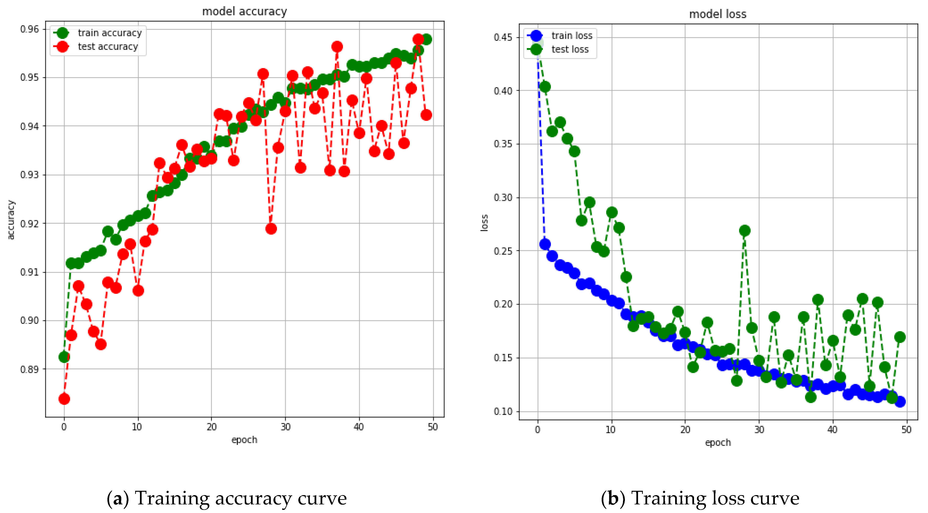
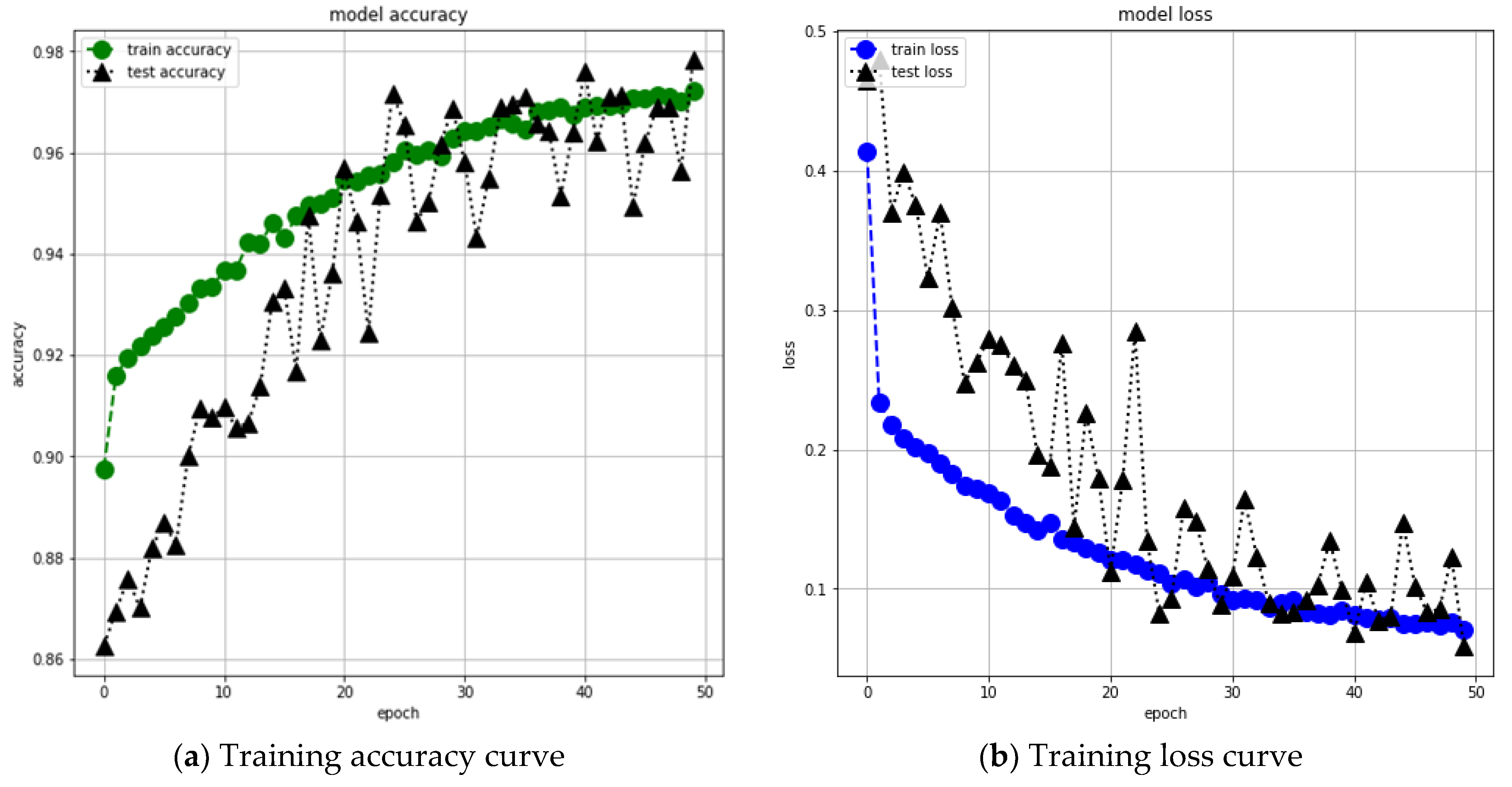
3. Experiments and Results Discussion

To implement Weed-ConvNet, the most effective architecture applies one or more stacks of convolution + pooling layers with suitable activation function, followed by a flatten layer and then finally one or two dense layers. The convolution neural network model with five convolution layers is designed for this weed plant classification problem. All these layers are followed by activation layers.

Batch normalization layers are used after activation layers. These normalization layers at each batch normalize the activations of the previous layer, i.e., converts the mean activation close to 0 and the activation standard deviation close to 1. Gaussian dropout layers are also applied after the max pooling layers. These dropout layers apply multiplicative 1-centered Gaussian noise. As it is a regularization layer, it remains active only at training time. The last layer is the dense layer with the SoftMax activation function.

Table 1. Layers of regularized Weed-ConvNet model.

Layer (Type)	Output Shape	Parameters
$\mathit{c}\mathit{o}\mathit{n}\mathit{v}\mathbf{2}\mathit{d}\_\mathbf{1} \left(\mathit{C}\mathit{o}\mathit{n}\mathit{v}\mathbf{2}\mathit{D}\right)$	$\left(\mathit{N}\mathit{o}\mathit{n}\mathit{e}, \mathbf{64}, \mathbf{64}, \mathbf{32}\right)$	$\mathbf{896}$
$\mathit{a}\mathit{c}\mathit{t}\mathit{i}\mathit{v}\mathit{a}\mathit{t}\mathit{i}\mathit{o}\mathit{n}\_\mathbf{1} \left(\mathit{R}\mathit{e}\mathit{L}\mathit{U}\right)$	$\left(\mathit{N}\mathit{o}\mathit{n}\mathit{e}, \mathbf{64}, \mathbf{64}, \mathbf{32}\right)$	$\mathbf{0}$
$\mathit{b}\mathit{a}\mathit{t}\mathit{c}\mathit{h}\_\mathit{n}\mathit{o}\mathit{r}\mathit{m}\mathit{a}\mathit{l}\mathit{i}\mathit{z}\mathit{a}\mathit{t}\mathit{i}\mathit{o}\mathit{n}\_\mathbf{1}$	$\left(\mathit{N}\mathit{o}\mathit{n}\mathit{e}, \mathbf{64}, \mathbf{64}, \mathbf{32}\right)$	$\mathbf{128}$
$\mathit{m}\mathit{a}\mathit{x}\_\mathit{p}\mathit{o}\mathit{o}\mathit{l}\mathit{i}\mathit{n}\mathit{g}\mathbf{2}\mathit{d}\_\mathbf{1}$	$\left(\mathit{N}\mathit{o}\mathit{n}\mathit{e}, \mathbf{32}, \mathbf{32}, \mathbf{32}\right)$	$\mathbf{0}$
$\mathit{g}\mathit{a}\mathit{u}\mathit{s}\mathit{s}\mathit{i}\mathit{a}\mathit{n}\_\mathit{d}\mathit{r}\mathit{o}\mathit{p}\mathit{o}\mathit{u}\mathit{t}\_\mathbf{1}$	$\left(\mathit{N}\mathit{o}\mathit{n}\mathit{e}, \mathbf{32}, \mathbf{32}, \mathbf{32}\right)$	$\mathbf{0}$
$\mathit{c}\mathit{o}\mathit{n}\mathit{v}\mathbf{2}\mathit{d}\_\mathbf{2} \left(\mathit{C}\mathit{o}\mathit{n}\mathit{v}\mathbf{2}\mathit{D}\right)$	$\left(\mathit{N}\mathit{o}\mathit{n}\mathit{e}, \mathbf{32}, \mathbf{32}, \mathbf{64}\right)$	$\mathbf{18496}$
$\mathit{a}\mathit{c}\mathit{t}\mathit{i}\mathit{v}\mathit{a}\mathit{t}\mathit{i}\mathit{o}\mathit{n}\_\mathbf{2} \left(\mathit{R}\mathit{e}\mathit{L}\mathit{U}\right)$	$\left(\mathit{N}\mathit{o}\mathit{n}\mathit{e}, \mathbf{32}, \mathbf{32}, \mathbf{64}\right)$	$\mathbf{0}$
$\mathit{b}\mathit{a}\mathit{t}\mathit{c}\mathit{h}\_\mathit{n}\mathit{o}\mathit{r}\mathit{m}\mathit{a}\mathit{l}\mathit{i}\mathit{z}\mathit{a}\mathit{t}\mathit{i}\mathit{o}\mathit{n}\_\mathbf{2}$	$\left(\mathit{N}\mathit{o}\mathit{n}\mathit{e}, \mathbf{32}, \mathbf{32}, \mathbf{64}\right)$	$\mathbf{256}$
$\mathit{m}\mathit{a}\mathit{x}\_\mathit{p}\mathit{o}\mathit{o}\mathit{l}\mathit{i}\mathit{n}\mathit{g}\mathbf{2}\mathit{d}\_\mathbf{2}$	$\left(\mathit{N}\mathit{o}\mathit{n}\mathit{e}, \mathbf{16}, \mathbf{16}, \mathbf{64}\right)$	$\mathbf{0}$
$\mathit{g}\mathit{a}\mathit{u}\mathit{s}\mathit{s}\mathit{i}\mathit{a}\mathit{n}\_\mathit{d}\mathit{r}\mathit{o}\mathit{p}\mathit{o}\mathit{u}\mathit{t}\_\mathbf{2}$	$\left(\mathit{N}\mathit{o}\mathit{n}\mathit{e}, \mathbf{16}, \mathbf{16}, \mathbf{64}\right)$	$\mathbf{0}$
$\mathit{c}\mathit{o}\mathit{n}\mathit{v}\mathbf{2}\mathit{d}\_\mathbf{3} \left(\mathit{C}\mathit{o}\mathit{n}\mathit{v}\mathbf{2}\mathit{D}\right)$	$\left(\mathit{N}\mathit{o}\mathit{n}\mathit{e}, \mathbf{16}, \mathbf{16}, \mathbf{128}\right)$	$\mathbf{73856}$
$\mathit{a}\mathit{c}\mathit{t}\mathit{i}\mathit{v}\mathit{a}\mathit{t}\mathit{i}\mathit{o}\mathit{n}\_\mathbf{3} \left(\mathit{R}\mathit{e}\mathit{L}\mathit{U}\right)$	$\left(\mathit{N}\mathit{o}\mathit{n}\mathit{e}, \mathbf{16}, \mathbf{16}, \mathbf{128}\right)$	$\mathbf{0}$
$\mathit{b}\mathit{a}\mathit{t}\mathit{c}\mathit{h}\_\mathit{n}\mathit{o}\mathit{r}\mathit{m}\mathit{a}\mathit{l}\mathit{i}\mathit{z}\mathit{a}\mathit{t}\mathit{i}\mathit{o}\mathit{n}\_\mathbf{3}$	$\left(\mathit{N}\mathit{o}\mathit{n}\mathit{e}, \mathbf{16}, \mathbf{16}, \mathbf{128}\right)$	$\mathbf{512}$
$\mathit{m}\mathit{a}\mathit{x}\_\mathit{p}\mathit{o}\mathit{o}\mathit{l}\mathit{i}\mathit{n}\mathit{g}\mathbf{2}\mathit{d}\_\mathbf{3}$	$\left(\mathit{N}\mathit{o}\mathit{n}\mathit{e}, \mathbf{8}, \mathbf{8}, \mathbf{128}\right)$	$\mathbf{0}$
$\mathit{g}\mathit{a}\mathit{u}\mathit{s}\mathit{s}\mathit{i}\mathit{a}\mathit{n}\_\mathit{d}\mathit{r}\mathit{o}\mathit{p}\mathit{o}\mathit{u}\mathit{t}\_\mathbf{3}$	$\left(\mathit{N}\mathit{o}\mathit{n}\mathit{e}, \mathbf{8}, \mathbf{8}, \mathbf{128}\right)$	$\mathbf{0}$
$\mathit{c}\mathit{o}\mathit{n}\mathit{v}\mathbf{2}\mathit{d}\_\mathbf{4} \left(\mathit{C}\mathit{o}\mathit{n}\mathit{v}\mathbf{2}\mathit{D}\right)$	$\left(\mathit{N}\mathit{o}\mathit{n}\mathit{e}, \mathbf{8}, \mathbf{8}, \mathbf{128}\right)$	$\mathbf{147584}$
$\mathit{a}\mathit{c}\mathit{t}\mathit{i}\mathit{v}\mathit{a}\mathit{t}\mathit{i}\mathit{o}\mathit{n}\_\mathbf{4} \left(\mathit{R}\mathit{e}\mathit{L}\mathit{U}\right)$	$\left(\mathit{N}\mathit{o}\mathit{n}\mathit{e}, \mathbf{8}, \mathbf{8}, \mathbf{128}\right)$	$\mathbf{0}$
$\mathit{b}\mathit{a}\mathit{t}\mathit{c}\mathit{h}\_\mathit{n}\mathit{o}\mathit{r}\mathit{m}\mathit{a}\mathit{l}\mathit{i}\mathit{z}\mathit{a}\mathit{t}\mathit{i}\mathit{o}\mathit{n}\_\mathbf{4}$	$\left(\mathit{N}\mathit{o}\mathit{n}\mathit{e}, \mathbf{8}, \mathbf{8}, \mathbf{128}\right)$	$\mathbf{512}$
$\mathit{c}\mathit{o}\mathit{n}\mathit{v}\mathbf{2}\mathit{d}\_\mathbf{5} \left(\mathit{C}\mathit{o}\mathit{n}\mathit{v}\mathbf{2}\mathit{D}\right)$	$\left(\mathit{N}\mathit{o}\mathit{n}\mathit{e}, \mathbf{8}, \mathbf{8}, \mathbf{256}\right)$	$\mathbf{295168}$
$\mathit{b}\mathit{a}\mathit{t}\mathit{c}\mathit{h}\_\mathit{n}\mathit{o}\mathit{r}\mathit{m}\mathit{a}\mathit{l}\mathit{i}\mathit{z}\mathit{a}\mathit{t}\mathit{i}\mathit{o}\mathit{n}\_\mathbf{5}$	$\left(\mathit{N}\mathit{o}\mathit{n}\mathit{e}, \mathbf{8}, \mathbf{8}, \mathbf{256}\right)$	$\mathbf{1024}$
$\mathit{g}\mathit{a}\mathit{u}\mathit{s}\mathit{s}\mathit{i}\mathit{a}\mathit{n}\_\mathit{d}\mathit{r}\mathit{o}\mathit{p}\mathit{o}\mathit{u}\mathit{t}\_\mathbf{4}$	$\left(\mathit{N}\mathit{o}\mathit{n}\mathit{e}, \mathbf{8}, \mathbf{8}, \mathbf{256}\right)$	$\mathbf{0}$
$\mathit{f}\mathit{l}\mathit{a}\mathit{t}\mathit{t}\mathit{e}\mathit{n}\_\mathbf{1} \left(\mathit{F}\mathit{l}\mathit{a}\mathit{t}\mathit{t}\mathit{e}\mathit{n}\right)$	$\left(\mathit{N}\mathit{o}\mathit{n}\mathit{e}, \mathbf{16384}\right)$	$\mathbf{0}$
$\mathit{d}\mathit{e}\mathit{n}\mathit{s}\mathit{e}\_\mathbf{1} \left(\mathit{D}\mathit{e}\mathit{n}\mathit{s}\mathit{e}\right)$	$\left(\mathit{N}\mathit{o}\mathit{n}\mathit{e}, \mathbf{1024}\right)$	$\mathbf{16778240}$
$\mathit{b}\mathit{a}\mathit{t}\mathit{c}\mathit{h}\_\mathit{n}\mathit{o}\mathit{r}\mathit{m}\mathit{a}\mathit{l}\mathit{i}\mathit{z}\mathit{a}\mathit{t}\mathit{i}\mathit{o}\mathit{n}\_\mathbf{6}$	$\left(\mathit{N}\mathit{o}\mathit{n}\mathit{e}, \mathbf{1024}\right)$	$\mathbf{4096}$
$\mathit{d}\mathit{e}\mathit{n}\mathit{s}\mathit{e}\_\mathbf{2} \left(\mathit{D}\mathit{e}\mathit{n}\mathit{s}\mathit{e}\right)$	$\left(\mathit{N}\mathit{o}\mathit{n}\mathit{e}, \mathbf{12}\right)$	$\mathbf{12300}$
$\mathit{a}\mathit{c}\mathit{t}\mathit{i}\mathit{v}\mathit{a}\mathit{t}\mathit{i}\mathit{o}\mathit{n}\_\mathbf{5} \left(\mathit{S}\mathit{o}\mathit{f}\mathit{t}\mathit{m}\mathit{a}\mathit{x}\right)$	$\left(\mathit{N}\mathit{o}\mathit{n}\mathit{e}, \mathbf{12}\right)$	$\mathbf{0}$
$\mathit{T}\mathit{r}\mathit{a}\mathit{i}\mathit{n}\mathit{a}\mathit{b}\mathit{l}\mathit{e} \mathit{p}\mathit{a}\mathit{r}\mathit{a}\mathit{m}\mathit{e}\mathit{t}\mathit{e}\mathit{r}\mathit{s}: \mathbf{17},\mathbf{329},\mathbf{804}$
$\mathit{N}\mathit{o}\mathit{n}-\mathit{t}\mathit{r}\mathit{a}\mathit{i}\mathit{n}\mathit{a}\mathit{b}\mathit{l}\mathit{e} \mathit{p}\mathit{a}\mathit{r}\mathit{a}\mathit{m}\mathit{e}\mathit{t}\mathit{e}\mathit{r}\mathit{s}: \mathbf{3},\mathbf{264}$

gives the details of each layer of the Weed-ConvNet model including output shape and parameters. Total trainable and non-trainable parameters are 17,329,804 and 3264, respectively.

To reduce the computation cost, the segmented images are cropped to size 64 × 64 from center. Data augmentation was performed over the cropped images. Over the cropped weed images, five main types of data augmentation techniques are used: image shifts with 1-pixel width and height shift range parameters, image flips with horizontal and vertical flip cases, image rotations with a 10-degree rotation range parameter, image brightness, and image zoom. The image dataset consists of total 5659 weed images. The dataset is divided into a 70% training dataset and a 30% testing dataset, i.e., 3961 and 1698 weed images in each category, respectively.

The learning parameters as provided in

Table 2. Learning parameters of Weed-ConvNet model.

Learning Parameter	Metric
Metric	$\mathrm{accuracy}$
Loss function	$\mathrm{categorical} \mathrm{cross} \mathrm{entropy}$
Optimizer	$\mathrm{adam}$

are applied to compile the model. The word metric in this table refers to how the model’s efficiency is calculated by classification accuracy. A loss function is a function that is used to calculate a loss value that the training method then attempts to reduce by adjusting the weights. The word optimizer refers to a method for determining how the network weights will be updated based on the loss function’s performance. The Adam optimization algorithm is one of the best optimization procedures available, and it works well with a variety of deep learning models.

The first step in the actual learning of the designed model is the fitting of the training data. Depending on the scale of the dataset, preparation takes up most of the time. An epoch is a complete transit of the training weed data through the learning algorithm. The algorithm’s epoch number is a significant hyperparameter. It defines the number of epochs or full passes through the algorithm’s learning phase for the training set. We partition the epoch into numerous smaller batches since one epoch is too large to provide to the computer all at once. The number of samples from the training set considered during each training iteration is referred to as the batch size. The weights are adjusted and the loss is calculated based on the batch size. The training process is completed with the total number of instances once after one epoch is finished. The validation dataset is used to evaluate the model’s learning performance. The training is repeated for the specified number of epochs. Stopping early and establishing the validation accuracy stabilization between consecutive epochs can improve this iteration. The learning hyperparameters that are used in this study are listed in

Table 3. Training hyperparameter optimization for Weed-ConvNet model.

Training Hyperparameter	Search Space	Selected Value
Learning rate	[0.1, 0.01, 0.001, 0.0001, 0.00001]	$0.001$
Epochs	[10, 20, 30, 40, 50, 60, 80, 100]	$50$
Batch size	[8, 16, 32, 64]	$32$
Early stopping	$parameter: va{l}_{loss}, patience \left[1,\mathrm{2.3.4.5}\right]$	$patience: 1$
Conv2D layer 1 channels	[8, 16, 32, 48]	[16]
Conv2D layer 2 channels	[8, 16, 32, 48]	[16]
Conv2D layer 3 channels	[16, 32, 48, 64, 128]	[32]
Conv2D layer 4 channels	[16, 32, 48, 64, 128]	[64]
Conv2D layer 5 channels	[16, 32, 48, 64, 128, 256]	[128]
Kernel size for layers	[1,2,3,4,5,6,7,8]	[8]
Padding	[0,1,2,3,4]	[0]
Conv2D stride	[1,2,3,4]	[2]
Dropout rate layer 1,2	[0.1, 0.2, 0.3, 0.4]	[0.2]
Dropout rate layer 1,2	[0.1, 0.2, 0.3, 0.4]	[0.4]

.

Two separate experiments were performed to measure the classification performance. In the first experiment, the grayscale segmented weed images are used, while in the second experiment, color segmented weed images are used. The same Weed-ConvNet model is utilized in both experiments. The training is repeated for 50 epochs in both cases. Figure 6 and Figure 7 display the training and testing accuracy and loss curves for weed plant classification with grayscale segmented weed images and color segmented weed images, respectively.

From the above curves, it is marked that there is a narrow difference between the training and the validation loss. This specifies that the network has learned the training data properly. These trained models neither overfitted nor underfitted means well regularized.

Table 4. Confusion matrix for Weed-ConvNet-based classification with grayscale segmented weed images.

Class	$\mathit{B}\mathit{l}\mathit{a}\mathit{c}\mathit{k}-\mathit{g}\mathit{r}\mathit{a}\mathit{s}\mathit{s}$	$\mathit{C}\mathit{h}\mathit{a}\mathit{r}\mathit{l}\mathit{o}\mathit{c}\mathit{k}$	$\mathit{C}\mathit{l}\mathit{e}\mathit{a}\mathit{v}\mathit{e}\mathit{r}\mathit{s}$	$\mathit{C}\mathit{o}\mathit{m}\mathit{m}\mathit{o}\mathit{n} \mathit{C}\mathit{h}\mathit{i}\mathit{c}\mathit{k}\mathit{w}\mathit{e}\mathit{e}\mathit{d}$	$\mathit{C}\mathit{o}\mathit{m}\mathit{m}\mathit{o}\mathit{n} \mathit{w}\mathit{h}\mathit{e}\mathit{a}\mathit{t}$	$\mathit{F}\mathit{a}\mathit{t} \mathit{H}\mathit{e}\mathit{n}$	$\mathit{L}\mathit{o}\mathit{o}\mathit{s}\mathit{e} \mathit{S}\mathit{i}\mathit{l}\mathit{k}\mathit{y}-\mathit{b}\mathit{e}\mathit{n}\mathit{t}$	$\mathit{M}\mathit{a}\mathit{i}\mathit{z}\mathit{e}$	$\mathit{S}\mathit{c}\mathit{e}\mathit{n}\mathit{t}\mathit{l}\mathit{e}\mathit{s}\mathit{s} \mathit{M}\mathit{a}\mathit{y}\mathit{w}\mathit{e}\mathit{e}\mathit{d}$	$\mathit{S}\mathit{h}\mathit{e}\mathit{p}\mathit{h}\mathit{e}\mathit{r}\mathit{d}\mathit{s} \mathit{P}\mathit{u}\mathit{r}\mathit{s}\mathit{e}$	$\mathit{S}\mathit{m}\mathit{a}\mathit{l}\mathit{l}-\mathit{f}\mathit{l}\mathit{o}\mathit{w}\mathit{e}\mathit{r}\mathit{e}\mathit{d} \mathit{C}\mathit{r}\mathit{a}\mathit{n}\mathit{e}\mathit{s}\mathit{b}\mathit{i}\mathit{l}\mathit{l}$	$\mathit{S}\mathit{u}\mathit{g}\mathit{a}\mathit{r} \mathit{b}\mathit{e}\mathit{e}\mathit{t}$
$Black-grass$	14	0	1	0	40	0	42	1	0	0	0	7
$Charlock$	0	123	4	0	3	2	0	0	0	0	0	6
$Cleavers$	0	7	74	0	12	5	0	0	0	8	4	4
$Common Chickweed$	0	20	10	102	1	5	0	13	3	5	1	60
$Common wheat$	0	0	2	0	62	1	2	1	1	0	0	4
$Fat Hen$	0	2	2	0	6	134	1	2	0	0	2	11
$Loose Silky-bent$	20	0	2	0	61	1	150	6	0	0	0	5
$Maize$	0	1	5	2	2	1	0	65	0	0	0	3
$Scentless Mayweed$	8	12	6	30	4	3	0	15	84	1	0	15
$Shepherd’s Purse$	0	19	2	4	3	1	0	0	4	25	0	3
$Small-flowered Cranesbill$	0	9	13	0	3	2	2	3	0	0	134	20
$Sugar beet$	0	3	0	0	6	1	0	10	0	0	1	118

presents the test results in terms of a confusion matrix for Weed-ConvNet-based classification with grayscale segmented weed images. A confusion matrix is a metric designed to assess the quality of a classification model. It is a square matrix whose dimensions the number of classes in a classifier determines. In this N × N matrix, rows denote to true classes and the columns signify the categorized class by the model.

Table 5. Confusion matrix for Weed-ConvNet-based classification with color segmented weed images.

Class	$\mathit{B}\mathit{l}\mathit{a}\mathit{c}\mathit{k}-\mathit{g}\mathit{r}\mathit{a}\mathit{s}\mathit{s}$	$\mathit{C}\mathit{h}\mathit{a}\mathit{r}\mathit{l}\mathit{o}\mathit{c}\mathit{k}$	$\mathit{C}\mathit{l}\mathit{e}\mathit{a}\mathit{v}\mathit{e}\mathit{r}\mathit{s}$	$\mathit{C}\mathit{o}\mathit{m}\mathit{m}\mathit{o}\mathit{n} \mathit{C}\mathit{h}\mathit{i}\mathit{c}\mathit{k}\mathit{w}\mathit{e}\mathit{e}\mathit{d}$	$\mathit{C}\mathit{o}\mathit{m}\mathit{m}\mathit{o}\mathit{n} \mathit{w}\mathit{h}\mathit{e}\mathit{a}\mathit{t}$	$\mathit{F}\mathit{a}\mathit{t} \mathit{H}\mathit{e}\mathit{n}$	$\mathit{L}\mathit{o}\mathit{o}\mathit{s}\mathit{e} \mathit{S}\mathit{i}\mathit{l}\mathit{k}\mathit{y}-\mathit{b}\mathit{e}\mathit{n}\mathit{t}$	$\mathit{M}\mathit{a}\mathit{i}\mathit{z}\mathit{e}$	$\mathit{S}\mathit{c}\mathit{e}\mathit{n}\mathit{t}\mathit{l}\mathit{e}\mathit{s}\mathit{s} \mathit{M}\mathit{a}\mathit{y}\mathit{w}\mathit{e}\mathit{e}\mathit{d}$	$\mathit{S}\mathit{h}\mathit{e}\mathit{p}\mathit{h}\mathit{e}\mathit{r}\mathit{d}\mathit{s} \mathit{P}\mathit{u}\mathit{r}\mathit{s}\mathit{e}$	$\mathit{S}\mathit{m}\mathit{a}\mathit{l}\mathit{l}-\mathit{f}\mathit{l}\mathit{o}\mathit{w}\mathit{e}\mathit{r}\mathit{e}\mathit{d} \mathit{C}\mathit{r}\mathit{a}\mathit{n}\mathit{e}\mathit{s}\mathit{b}\mathit{i}\mathit{l}\mathit{l}$	$\mathit{S}\mathit{u}\mathit{g}\mathit{a}\mathit{r} \mathit{b}\mathit{e}\mathit{e}\mathit{t}$
$\mathit{B}\mathit{l}\mathit{a}\mathit{c}\mathit{k}-\mathit{g}\mathit{r}\mathit{a}\mathit{s}\mathit{s}$	46	0	0	0	4	4	44	0	0	0	2	5
$\mathit{C}\mathit{h}\mathit{a}\mathit{r}\mathit{l}\mathit{o}\mathit{c}\mathit{k}$	1	130	2	0	1	2	0	0	0	0	0	2
$\mathit{C}\mathit{l}\mathit{e}\mathit{a}\mathit{v}\mathit{e}\mathit{r}\mathit{s}$	0	6	99	0	1	3	0	0	0	0	0	5
$\mathit{C}\mathit{o}\mathit{m}\mathit{m}\mathit{o}\mathit{n} \mathit{C}\mathit{h}\mathit{i}\mathit{c}\mathit{k}\mathit{w}\mathit{e}\mathit{e}\mathit{d}$	0	1	0	210	2	1	0	3	0	0	1	2
$\mathit{C}\mathit{o}\mathit{m}\mathit{m}\mathit{o}\mathit{n} \mathit{w}\mathit{h}\mathit{e}\mathit{a}\mathit{t}$	2	0	1	1	53	5	1	0	2	0	0	8
$\mathit{F}\mathit{a}\mathit{t} \mathit{H}\mathit{e}\mathit{n}$	0	0	2	1	0	154	0	0	0	0	2	1
$\mathit{L}\mathit{o}\mathit{o}\mathit{s}\mathit{e} \mathit{S}\mathit{i}\mathit{l}\mathit{k}\mathit{y}-\mathit{b}\mathit{e}\mathit{n}\mathit{t}$	35	1	1	0	5	9	185	1	0	0	3	5
$\mathit{M}\mathit{a}\mathit{i}\mathit{z}\mathit{e}$	0	0	0	0	1	0	0	77	0	0	0	1
$\mathit{S}\mathit{c}\mathit{e}\mathit{n}\mathit{t}\mathit{l}\mathit{e}\mathit{s}\mathit{s} \mathit{M}\mathit{a}\mathit{y}\mathit{w}\mathit{e}\mathit{e}\mathit{d}$	3	3	1	7	0	1	0	2	155	1	0	5
$\mathit{S}\mathit{h}\mathit{e}\mathit{p}\mathit{h}\mathit{e}\mathit{r}\mathit{d}’\mathit{s} \mathit{P}\mathit{u}\mathit{r}\mathit{s}\mathit{e}$	0	3	0	2	0	1	0	0	1	52	0	2
$\mathit{S}\mathit{m}\mathit{a}\mathit{l}\mathit{l}-\mathit{f}\mathit{l}\mathit{w}. \mathit{C}\mathit{r}\mathit{a}\mathit{n}\mathit{e}\mathit{s}\mathit{b}\mathit{i}\mathit{l}\mathit{l}$	0	2	2	0	1	1	0	0	2	0	176	2
$\mathit{S}\mathit{u}\mathit{g}\mathit{a}\mathit{r} \mathit{b}\mathit{e}\mathit{e}\mathit{t}$	0	1	0	0	0	1	0	2	0	0	3	132

presents the results in terms of a confusion matrix for Weed-ConvNet-based classification with color segmented weed images. By comparing the confusion matrices, it can be observed that the color segmented weed images give low false classifications.

Output metrics are measured using the above confusion matrices to further test the qualified models. Precision, recall, and the F1 score are all used as performance indicators. The proportion of accurate predictions to total predictions is defined as classification accuracy. Precision is described as the proportion of correct predictions to the total number of correct predictions expected. This metric assesses the classifier’s ability to predict positive outcomes. The ratio of correct positive predictions to total positive predictions is referred to as sensitivity or recall. The F1 score combines precision and recall in relation to a specific positive class. The F1 score is a weighted average of recall and precision, with one signifying the best and zero representing the worst [27]. These metrics are specified below.

$$\mathrm{Precision}=\frac{Tru{e}^{+}}{Tru{e}^{+}+Fals{e}^{+}}$$

(6)

$$\mathrm{Sensitivity}=\frac{Tru{e}^{+}}{Tru{e}^{+}+Fals{e}^{-}}$$

(7)

$$\mathrm{F}1-\mathrm{Score}=\frac{2*\mathrm{Precision}*\mathrm{Sensitivity}}{\mathrm{Precision}+\mathrm{Sensitivity}}$$

(8)

$$\mathrm{Accuracy}=\frac{Tru{e}^{+}+Tru{e}^{-}}{Tru{e}^{+}+Tru{e}^{-}+Fals{e}^{-}+Fals{e}^{+}}$$

(9)

where:

• $Tru{e}^{+}$ and $Tru{e}^{-}$ are the truly labelled positive and negative weed samples, respectively.
• $Fals{e}^{+}$ represents the no. of negative weed samples labelled incorrectly as positive.
• $Fals{e}^{-}$ denotes the no. of positive weed samples labelled incorrectly as negative.

Table 6. Performance metrics for regularized Weed-ConvNet-based classification with grayscale and color segmented weed images.

Class	Performance Measures with Grayscale Segmented Weed Images			Performance Measures with Color Segmented Weed Images
	Precision	Recall	F1 Score	Precision	Recall	F1 Score
Black-grass	0.33	0.13	0.19	0.53	0.44	0.48
Charlock	0.63	0.89	0.74	0.88	0.94	0.91
Cleavers	0.61	0.65	0.63	0.92	0.87	0.89
Common chickweed	0.74	0.46	0.57	0.95	0.95	0.95
Common wheat	0.31	0.85	0.45	0.78	0.73	0.75
Fat hen	0.86	0.84	0.85	0.85	0.96	0.9
Loose silky-bent	0.76	0.61	0.68	0.8	0.76	0.78
Maize	0.56	0.82	0.67	0.91	0.97	0.94
Scentless mayweed	0.91	0.47	0.62	0.97	0.87	0.92
Shepherd’s purse	0.64	0.41	0.5	0.98	0.85	0.91
Small-flowered cranesbill	0.94	0.72	0.82	0.94	0.95	0.94
Sugar beet	0.46	0.85	0.6	0.78	0.95	0.85
Average	0.7	0.64	0.64	0.86	0.87	0.86
Test Loss	0.169			0.059
Test Accuracy	0.942			0.978

consists of these measures. These three performance measures are higher in color segmented weed images which are 0.86, 0.87, and 0.86 respectively. The test accuracy of the Weed-ConvNet model with the color segmented weed images is 0.978, which is better than 0.942 of the Weed-ConvNet model with the grayscale segmented weed images.

Figure 8 displays the ROC curves to affirm the robustness of these weed plant classification problems. ROC analysis is a graphical method for analyzing a classifier’s performance. It characterizes a classifier’s performance using two statistics: true positive rate (TPR) and false positive rate (FPR). The x-axis of a ROC curve normally shows the FPR, while the y-axis displays the TPR. This means that the plot’s top left corner is the “ideal” point, with a TPR of one and a FPR of zero. This implies that having a larger area under the curve (AUC) is generally better. These ROC plots show that the Weed-ConvNet model with color segmented weed images outperforms greyscale segmented weed images, as indicated by the area under curves of these curves.

ROC plots are commonly used in binary classification to investigate a classifier’s performance. Binarizing the output is needed to extend the ROC plot and AUC to multi-label or multi-class problems. Micro-averaging is a binarized plot in which the ROC is plotted by treating each member of the label matrix as a binary classification. Tang et al. developed an alternative multi-class label evaluation metric that delivers the same weight to each class label (2014). As shown in these ROC curves, for the first Weed-ConvNet model, the micro-average area and macro-average area are 09.4 and 0.96, respectively. With the color segmented weed images, the metrics micro-average area and macro-average area improve to 0.99 in each case.

4. Conclusions

IOT technology-based smart farming can empower cultivators and farmers to decrease waste and improve production. With the help of an IOT-based system for monitoring the crop field, crops can be improved with the help of humidity, light, image, temperature, and moisture sensors. Out of these sensors, an image-acquisition-enabled IOT device plays a vital role. This work discussed a case study where image processing and IOT played an important role for weed plant seedling detection and classification. The early detection of weed seedling can enable farmers to use herbicides or other control mechanisms on time. The regularized Weed-ConvNet is made to classify weed images that have been colored and gray scaled. The Weed-ConvNet model’s accuracy with color segmented weed images is 0.978, which is higher than the model’s accuracy with grayscale segmented weed images of 0.942. In future, it will be vital to determine that on which crops can an IOT-enabled model be applied to, since weeds spread amongst different crops. It might not be able to distinguish some weeds from crops since they resemble them so closely. Additionally, the density of plant seeding, stage of plant development, and other aspects will have a big impact on the IOT-enabled model’s ability to identify weeds.

References

1. Gubbi, J.; Buyya, R.; Marusic, S.; Palaniswami, M. Internet of Things (IoT): A vision, architectural elements, and future directions. Future Gener. Comput. Syst. 2013, 29, 1645–1660. [Google Scholar] [CrossRef] [Green Version]
2. Lee, I.; Lee, K. The Internet of Things (IoT): Applications, investments, and challenges for enterprises. Bus. Horiz. 2015, 58, 431–440. [Google Scholar] [CrossRef]
3. Goenka, N.; Tiwari, S. AlzVNet: A volumetric convolutional neural network for multiclass classification of Alzheimer’s disease through multiple neuroimaging computational approaches. Biomed. Signal Process. Control 2022, 74, 103500. [Google Scholar] [CrossRef]
4. Litjens, G.; Kooi, T.; Bejnordi, B.E.; Setio, A.A.A.; Ciompi, F.; Ghafoorian, M.; Sánchez, C.I. A survey on deep learning in medical image analysis. Med. Image Anal. 2017, 42, 60–88. [Google Scholar] [CrossRef] [PubMed] [Green Version]
5. Lipper, L.; Thornton, P.; Campbell, B.M.; Baedeker, T.; Braimoh, A.; Bwalya, M.; Hottle, R. Climate-smart agriculture for food security. Nat. Clim. Change 2014, 4, 1068. [Google Scholar] [CrossRef]
6. Sinha, B.B.; Dhanalakshmi, R. Recent advancements and challenges of Internet of Things in smart agriculture: A survey. Future Gener. Comput. Syst. 2022, 126, 169–184. [Google Scholar] [CrossRef]
7. Adamides, G.; Edan, Y. Human–robot collaboration systems in agricultural tasks: A review and roadmap. Comput. Electron. Agric. 2023, 204, 107541. [Google Scholar] [CrossRef]
8. Gondchawar, N.; Kawitkar, R.S. IoT based smart agriculture. Int. J. Adv. Res. Comput. Commun. Eng. 2016, 5, 838–842. [Google Scholar]
9. TongKe, F. Smart agriculture based on cloud computing and IOT. J. Converg. Inf. Technol. 2013, 8, 210–216. [Google Scholar]
10. Jhuria, M.; Kumar, A.; Borse, R. Image processing for smart farming: Detection of disease and fruit grading. In Proceedings of the 2013 IEEE Second International Conference on Image Information Processing (ICIIP-2013), Shimla, India, 9–11 December 2013; pp. 521–526. [Google Scholar]
11. Bhange, M.; Hingoliwala, H.A. Smart farming: Pomegranate disease detection using image processing. Procedia Comput. Sci. 2015, 58, 280–288. [Google Scholar] [CrossRef] [Green Version]
12. Hamuda, E.; Glavin, M.; Jones, E. A survey of image processing techniques for plant extraction and segmentation in the field. Comput. Electron. Agric. 2016, 125, 184–199. [Google Scholar] [CrossRef]
13. Mekala, M.S.; Viswanathan, P. A Survey: Smart agriculture IoT with cloud computing. In Proceedings of the 2017 International Conference on Microelectronic Devices, Circuits and Systems (ICMDCS), Vellore, India, 10–12 August 2017; pp. 1–7. [Google Scholar]
14. Suma, N.; Samson, S.R.; Saranya, S.; Shanmugapriya, G.; Subhashri, R. IOT based smart agriculture monitoring system. Int. J. Recent Innov. Trends Comput. Commun. 2017, 5, 177–181. [Google Scholar]
15. Kapoor, A.; Bhat, S.I.; Shidnal, S.; Mehra, A. Implementation of IoT (Internet of Things) and Image processing in smart agriculture. In Proceedings of the 2016 International Conference on Computation System and Information Technology for Sustainable Solutions (CSITSS), Bengaluru, India, 6–8 October 2016; pp. 21–26. [Google Scholar]
16. Lottes, P.; Khanna, R.; Pfeifer, J.; Siegwart, R.; Stachniss, C. UAV-based crop and weed classification for smart farming. In Proceedings of the 2017 IEEE International Conference on Robotics and Automation (ICRA), Singapore, 29 May–3 June 2017; pp. 3024–3031. [Google Scholar]
17. Sadjadi, F.A.; Farmer, M.E. Smart Weed Recognition/Classification System. U.S. Patent No. 5,606,821, 4 March 1997. [Google Scholar]
18. Dang, M.P.; Le, H.G.; Le Chau, N.; Dao, T.P. An Optimized Design of New XYθ Mobile Positioning Microrobotic Platform for Polishing Robot Application Using Artificial Neural Network and Teaching-Learning Based Optimization. Complexity 2022, 2022, 2132005. [Google Scholar] [CrossRef]
19. Dang, M.P.; Le, H.G.; Nguyen, N.P.; Le Chau, N.; Dao, T.P. Optimization for a New XY Positioning Mechanism by Artificial Neural Network-Based Metaheuristic Algorithms. Comput. Intell. Neurosci. 2022, 2022, 9151146. [Google Scholar] [CrossRef]
20. LeCun, Y.; Bengio, Y.; Hinton, G. Deep learning. Nature 2015, 521, 436. [Google Scholar] [CrossRef] [PubMed]
21. Sharma, A.K.; Tiwari, S.; Aggarwal, G.; Goenka, N.; Kumar, A.; Chakrabarti, P.; Jasiński, M. Dermatologist-Level Classification of Skin Cancer Using Cascaded Ensembling of Convolutional Neural Network and Handcrafted Features Based Deep Neural Network. IEEE Access 2022, 10, 17920–17932. [Google Scholar] [CrossRef]
22. Tiwari, S. An analysis in tissue classification for colorectal cancer histology using convolution neural network and colour models. Int. J. Inf. Syst. Model. Des. 2018, 9, 1–19. [Google Scholar] [CrossRef]
23. Tripathi, N.; Jadeja, A. A survey of regularization methods for deep neural network. Int. J. Comput. Sci. Mob. Comput. 2014, 3, 429–436. [Google Scholar]
24. Mikołajczyk, A.; Grochowski, M. Data augmentation for improving deep learning in image classification problem. In Proceedings of the 2018 International Interdisciplinary PhD Workshop (IIPhDW), Swinoujście, Poland, 9–12 May 2018; pp. 117–122. [Google Scholar]
25. Alimboyong, C.R.; Hernandez, A.A. An Improved Deep Neural Network for Classification of Plant Seedling Images. In Proceedings of the 2019 IEEE 15th International Colloquium on Signal Processing & Its Applications (CSPA), Penang, Malaysia, 8–9 March 2019; pp. 217–222. [Google Scholar]
26. Giselsson, T.M.; Jørgensen, R.N.; Jensen, P.K.; Dyrmann, M.; Midtiby, H.S. A public image database for benchmark of plant seedling classification algorithms. arXiv 2017, arXiv:1711.05458. [Google Scholar]
27. Tiwari, S. A Pattern Classification Based approach for Blur Classification. Indones. J. Electr. Eng. Inform. 2017, 5, 162–173. [Google Scholar]
28. Ramani, P.; Pradhan, N.; Sharma, A.K. Classification Algorithms to Predict Heart Diseases—A Survey. In Computer Vision and Machine Intelligence in Medical Image Analysis. Advances in Intelligent Systems and Computing; Gupta, M., Konar, D., Bhattacharyya, S., Biswas, S., Eds.; Springer: Singapore, 2020; Volume 992. [Google Scholar]
29. Sharma, N.; Litoriya, R.; Sharma, A. Application and Analysis of K-Means Algorithms on a Decision Support Framework for Municipal Solid Waste Management. In Advanced Machine Learning Technologies and Applications. AMLTA 2020. Advances in Intelligent Systems and Computing; Hassanien, A., Bhatnagar, R., Darwish, A., Eds.; Springer: Singapore, 2021; Volume 1141. [Google Scholar]
30. Tang, K.; Wang, R.; Chen, T. Towards maximizing the area under the ROC curve for multi-class classification problems. In Proceedings of the Twenty-Fifth AAAI Conference on Artificial Intelligence, San Francisco, CA, USA, 7–11 August 2011. [Google Scholar]
31. Le Chau, N.; Tran, N.T.; Dao, T.P. Topology and size optimization for a flexure hinge using an integration of SIMP, deep artificial neural network, and water cycle algorithm. Appl. Soft Comput. 2021, 113, 108031. [Google Scholar] [CrossRef]
Figure 1. (a): A typical model of IOT-based image analytics for smart agriculture [13]. (b): Layered architecture for IOT-enabled smart agriculture consisting of a crop collection layer, sensory layer, analytical/cloud layer, and a prediction layer.
Agriengineering 05 00017 g001
Figure 2. Flow graph of the entire system.
Agriengineering 05 00017 g002
Figure 3. Architecture of the Weed-ConvNet model.
Agriengineering 05 00017 g003
Figure 4. Weed plant image dataset samples.
Agriengineering 05 00017 g004
Figure 5. Segmented weed plant image dataset samples.
Agriengineering 05 00017 g005
Figure 6. Training and testing accuracy and loss curves for weed plant classification with grayscale segmented weed images.
Agriengineering 05 00017 g006
Figure 7. Training and testing accuracy and loss curves for weed plant classification with color segmented weed images.
Agriengineering 05 00017 g007
Figure 8. Receiver operating characteristic curves: (a) experiment with grayscale segmented weed images; (b) experiment with grayscale segmented weed images.
Agriengineering 05 00017 g008