
Autonomous Vineyard Tracking Using a Four-Wheel-Steering Mobile Robot and a 2D LiDAR
by
 ,
,
Dimia Iberraken
1,* ,
,
Florian Gaurier
1,
Jean-Christophe Roux
1,
Colin Chaballier
2 and
Roland Lenain
1 1
INRAE, UR TSCF, Université Clermont Auvergne, F-63000 Clermont-Ferrand, France
2
Exxact Robotics, F-51200 Épernay, France
*
Author to whom correspondence should be addressed.
AgriEngineering 2022, 4(4), 826-846; https://doi.org/10.3390/agriengineering4040053
Submission received: 31 July 2022
/
Revised: 13 September 2022
/
Accepted: 18 September 2022
/
Published: 22 September 2022
(This article belongs to the Special Issue Selected Papers from The Ag Robotic Forum—World FIRA 2021)
Abstract
:The intensive advances in robotics have deeply facilitated the accomplishment of tedious and repetitive tasks in our daily lives. If robots are now well established in the manufacturing industry, thanks to the knowledge of the environment, this is still not fully the case for outdoor applications such as in agriculture, as many parameters are varying (kind of vegetation, perception conditions, wheel–soil interaction, etc.) The use of robots in such a context is nevertheless important since the reduction of environmental impacts requires the use of alternative practices (such as agroecological production or organic production), which require highly accurate work and frequent operations. As a result, the design of robots for agroecology implies notably the availability of highly accurate autonomous navigation processes related to crop and adapting to their variability. This paper proposes several contributions to the problem of crop row tracking using a four-wheel-steering mobile robot, which straddles the crops. It uses a 2D LiDAR allowing the detection of crop rows in 3D thanks to the robot motion. This permits the definition of a reference trajectory that is followed using two different control approaches. The main targeted application is navigation in vineyard fields, to achieve several kinds of operation, such as monitoring, cropping, or accurate spraying. In the first part, a row detection strategy based on a 2D LiDAR inclined in front of the robot to match a predefined shape of the vineyard row in the robot framework is described. The successive detected regions of interest are aggregated along the local robot motion, through the system odometry. This permits the computation of a local trajectory to be followed by a robot. In a second part, a control architecture that allows the control of a four-wheel-steering mobile robot is proposed. Two different strategies are investigated, one is based on a backstepping approach, while the second considers independently the regulation of front and rear steering axle position. The results of these control laws are then compared in an extended simulation framework, using a 3D reconstruction of actual vineyards in different seasons.
1. Introduction
Autonomous navigation of off-road robots arises as a central question for the ecological transition of agriculture in the framework of vine production. Required chemicals reduction, together with the use of bio-control products, leads to increasing the accuracy of tasks to be achieved, as well as the frequency of field interventions. The lack of manpower and the painfulness of such tasks promote the development of autonomous robots, especially those working in vineyards. Indeed, more and more agricultural robots are deployed in farms in order to relieve the work of the farmer by reducing the drudgery of certain manual tasks [1]. The role of these robots does not end there, they also allow a better agricultural yield, reduce the exposure of workers to certain chemical products sprayed on the plantations, and allow a more efficient and precise agriculture. Indeed, navigation in vineyards requires a centimeter-level accuracy with respect to the vegetation, especially on a straddle robot. Solutions that are based on Global Navigation Satellite System (GNSS) that can provide precise localization technology with real-time kinematic (RTK) corrections allows this kind of precision, as shown in previous authors’ work [2,3]. However, this implies a prior definition of a global path allowing to integrate the vineyard row information. Generating a trajectory using prior information of the environment can be performed through a collection phase of way-points along the field. The reference path is then provided as a global path created by manually surveying the field using RTK-GNSS. The absolute localization provided by the RTK-GNSS system is then considered as the ground truth [4,5]. The precise localization of the robot is derived by the fusion of the RTK-GNSS and additional sensors such as the odometry of the robot and an IMU, while using the most commonly used tool—a Kalman Filter [6,7,8], for instance. This also has the advantage of overcoming the eventual loss of GPS signal in large canopies, especially in vineyard, orchard applications, greenhouses, or when experiencing signal perturbations [9].
Line detection from row crop fields emerges as an alternative solution to RTK-GNSS navigation. This technique differs in the type of data used (e.g., point-cloud or images) and in the line-fitting algorithm (e.g., RANSAC (RANdom SAmple Consensus) [10,11] or Hough transform [12,13]), but also in the used sensor (Vision-based [14,15,16] or LiDAR-based [4,10,17,18]).
Vision sensors are often exploited in order to extract the parallel lines in the crop structure from the input data. For example, Hough transform from images is often used as a line-fitting method. However, the method is not robust to uncertainty and can extract incorrect lines that lead to navigation failure. Moreover, it is classically performed under the assumption of prior knowledge of the field such as row spacing or the number of crop rows [19,20], and it is sensitive to the environment with a significant presence of weeds or dense canopy. In an effort to increase robustness, [13] proposes an approach to detect crop row patterns in a single step instead of detecting individual lines. However, vision-based sensors come with the disadvantage of being sensitive to lighting conditions, which is a major drawback in outdoor applications. LiDAR-based navigation methods, on the other hand, overcome this drawback and also have the advantage of high resolution and large field of view, especially in outdoor applications. In [4], a multi-layer LiDAR (Ouster 16-channel) is used in order to extract the row line using Hough transform. This is performed with a parameterization based on point-cloud statistics to extract useful structure parameters such as the number of rows input to the Hough transform algorithm. However, the use of such 3D sensor appears to be costly regarding the task of structure tracking. Hybrid solutions allows to have the best of multiple sensor solutions. The solution proposed in [21] makes use of a laser range finder and RGBD device and a GPS. The laser range finder and RGBD device are used to perform reactive row following and obstacle avoidance, while GPS navigation is used for changing from row to row or field to field. In this paper, we favor the use of a less expensive sensor, a 2D-LiDAR laser scanner, as we believe it is a sufficient sensor solution for structure tracking.
Once a path is extracted with respect to crops, different control strategies are used in the framework of path following. Even when the robot is subject to perturbations such as sliding or non-ideal actuators, the motion still needs to be precisely controlled. Additionally, the robots must perform maneuvers in crowded areas with limited space and under heterogeneous terrain conditions [22]. To address this issue in the context of our application, robots equipped with four independent steering wheels (called 4WS robots) arise as a good solution to have more degrees of freedom. This allows to increase the agility and maneuverability, while controlling independently the robot position and orientation, with respect to the row. Indeed, this kind of robot offers a great range of movements and allows a reduction of the radius of curvature, especially when moving in narrow spaces such as encountered in vineyards or when carrying a tool, such as in spraying applications [23], but it also allows compensating for sideslip angles. As for the control of 4WS robots, the objective in the classical approaches for path tracking [24] is to linearize the kinematic model of the robot in order to obtain an expression of the control (i.e., the steering angle of the robot), which guarantees the convergence of the lateral deviation towards the desired one. The exact linearization approach has the advantage of providing a mathematical expression giving at any time the ideal control depending on the robot state measurement. Moreover, thanks to the integration of gains in this expression, it is possible to adjust the dynamics of the robot by defining a time or a convergence distance of the robot towards the target trajectory. This solution is efficient and accurate, but it only allows to set the time (or the distance) of convergence to the trajectory. This approach is generally sufficient when moving in an open environment; in the case of structure tracking, it can become limiting. Indeed, in order to guarantee tracking of a structure without collision with it, it can be interesting to control more efficiently the convergence of the robot towards the structure and in particular its orientation. The work in [25] investigates the possibility of accurately controlling a 4WS with respect to a path, while maintaining different desired absolute orientations with respect to the global frame and guaranteeing different desired lateral deviations. However, depending on the application, the absolute orientation is not always obtainable.
In this paper, a robust 2D LiDAR-based solution is chosen in order to navigate reactively in the vine field while allowing to account for the variability of lightning, weather conditions, and the evolution of vegetation. Indeed, we are interested in studying the generecity of a reactive LiDAR-based navigation strategy throughout the seasons. For this reason, a GPS free solution is proposed as in the proposed work field, the task is tied to the evolution of vegetation rather than to a specific positioning. The approach consists of detecting the expected structure shape of a vine in each laser scan and aggregating the successive scans into a global map, in the vicinity of the robot’s position. The accumulation of points in 3D space during the robot’s movement will then define the trajectory to follow. The proposed navigation algorithm allows a 4WS mobile robot to work on vineyards, despite the evolution of vegetation toward different seasons. In addition, it is proposed to illustrate the well-working of the navigation algorithm through two different control strategies. The first strategy presented considers a backstepping approach to independently control the longitudinal and lateral controls and thus separate the regulation of the position and the orientation of the robot. The second strategy presented considers separating control of the front axle and the rear axle, to ensure they follow the same path.
This paper is organized as follows. First, the row tracking strategy is detailed in Section 2.1. Then, the control framework is detailed in Section 2.2, where two control strategies are detailed to illustrate the path tracking. Section 3 presents the simulation results on an advanced simulation testbed (3D reconstruction of actual vineyard in different seasons) to illustrate the efficiency of the proposed structure detection algorithm as well as the two control strategies. Finally, Section 4 concludes the paper and presents some insights for future works.
2. Materials and Methods
Throughout this section, the methods used to conduct this research are detailed. First, the row tracking strategy is described in Section 2.1, involving the use of a 2D LiDAR sensor. This allows the computation of a local reference trajectory to be followed. Secondly, the used motion control strategies are detailed in Section 2.2. These strategies allow accurate tracking of lateral and angular deviation with respect to the detected structure. Lastly, the proposed control architecture is tested on an advanced simulation testbed composed of a digitized vineyard in two different field configurations related to plant growth.
2.1. Row Detection Strategy
The overall procedure is shown in Figure 1.
The row detection strategy defined in this work is firstly based on finding crop shape matching an expected model within the LiDAR framework. The idea was initiated in the author’s previous work [26] where the purpose was to detect the footprint left by tires from a previous operation on the field. In our case, the goal in this work is to follow a trajectory defined by the vineyard structure with an autonomous mobile robot, using an inclined 2D LiDAR. The LiDAR is set at the top front of the robot in order to see above the vine to limit the masking effect (cf. Figure 2 of the robot TRAXX by Exxact Robotics, available online: https://exxact-robotics.com/produit/traxx (accessed on 22 September 2022)). A pitch angle is also set on the LiDAR to extend the distance of prediction of the system.
The approach consists then of detecting the expected structure shape in each laser scan and aggregating the successive scans into a global map. The accumulation of points in 3D space during the robot’s movement will then define the trajectory to follow.
2.1.1. Pre-Processing
The objective here is to extract the set of LiDAR set-points that are the most representative for row tracking. The first step consists of reducing the field of view of the LiDAR in order to reduce the research area to the closest rows. This is performed by keeping the data that belongs to the range [−30°, 30°]. Then, ground variations are removed in order to compensate for soil inclination present in an uneven terrain of an off-road context, contrary to the expected model of the vine that is defined on a flat and even surface. Therefore, a preliminary step is to estimate the general profile of the terrain in order to compensate for the inclination of the ground. This is achieved using the RANSAC algorithm [27]. This allows the elimination of large variations in the ground and inclinations without minimizing the other variations representative of the structure of the model. Figure 3 shows an example of this correction on a simulated uneven terrain.
2.1.2. Detection Model Definition
Once the general soil inclination has been compensated, the adequate model of a single grapevine is defined. As shown in Figure 4a, when using 2D laser scanner, the vine can be approximated by a squared signal whose minimum is set to the ground. The height of such a model is defined to be the typical height of a vine. The width is tied to the density of the plant cover. Therefore, the width is smaller in a winter vineyard and larger in a summer vineyard. An example of simulated LiDAR data and its model is shown in Figure 4a.
2.1.3. Correlation Score Definition
The objective is then to find the matching shape of the vine model in the data returned by the LiDAR. To this end, a correlation between the current LiDAR scan and the previously generated model is computed. In order to find the position of an expected vine, this score is computed from a moving offset k in the point index. By denoting N the number of impact points retrieved from the laser beam, then k will move in between to , to find the offset that fits the best with the model. An example of results can be seen in Figure 5a, showing the correlation score with respect to the offset. Figure 5b shows then the superposition between the point cloud and the vine model at the index k, where the correlation score is maximal. Assuming that the model and the laser measurement have the same number of points, the correlation expression used is defined by:
With:
- is the correlation score for the offset k between LiDAR data and template;
- z represents the LiDAR measurements on the Z-axis;
- m represents the values of the model data;
- and are the mean values of, respectively, LiDAR Z-axis data and model data.
Since Equation (1) is normalized, the global maximum of the correlation can be retrieved and compared to a threshold value, empirically defined ensuring less false detection (cf. Figure 5a). Then, the correlation maximum is associated to its corresponding value in the LiDAR signal as shown on Figure 5b.
At this step, each maximum of the correlation score above the threshold (as depicted in Figure 5a) can be considered as a candidate for vine detection. At each LiDAR acquisition, one can then find zero or several candidates. In the next section, we will see how a new detected point can be classified as a good detection and aggregated with the previous set-points.
2.1.4. Vine Structure Reconstruction
The purpose of this application is to follow a trajectory defined by a structure of the vineyard with an autonomous mobile robot, thanks to LiDAR detection. The approach is then to detect the expected structure in each laser scan and aggregate the successive scans into an overall map. Points accumulation in 3D space during the movement of the robot will then define the trajectory to follow. The previously retrieved set-point in the LiDAR signal is the set-point where the model suits the best data (cf. Figure 5b). To classify it as a selected set-point for aggregation to the reference trajectory, its distance to the previously aggregated set-point has to be computed. Hence, the retrieved set-point is expressed in the global frame using the localization of the robot. In this case, robot odometry is used. The impact of the drift of such a sensor is limited by a distance removal criterion between the oldest set-point and the robot location. In fact, the drift in the use of this type of data will not affect the accuracy of the trajectory tracking, since only a local part will be used to evaluate the lateral and angular deviations. Indeed, only the data between the impact of the LiDAR and the robot’s tires are kept; this distance of a few meters is not significantly impacted by the drift of the odometry. The retrieved set-point, now expressed in the global frame, is compared to the newest set-point using the following formula:
With:
- —the lateral deviation of the retrieved point to the newest set-point in the robot frame;
- —the yaw of the robot computed with the odometry;
- and —the X and Y coordinates of the retrieved point;
- and —the X and Y coordinates of the previous aggregated set-point.
If the computed distance is low enough, the point is considered as a set-point and agglomerated with the others, as shown in Figure 6.
2.1.5. Trajectory Computation and Input Control
To match the structure of the vine row, the trajectory is computed using a mean least squares method, as shown in Figure 6. The detected points represent a local line approximation of the vine row (assuming low variation in the curvature of the vine structure). Once the reference trajectory is obtained, it is used to compute the lateral and angular deviation as inputs to the control law. The lateral and angular deviations with respect to the linear estimation of the trajectory given by the expression are computed as follows:
With:
- y—the lateral deviation with respect to the reference trajectory;
- a and b, respectively, the slope and intercept computed by the least squares method;
- and —the coordinates of the robot computed through the system odometry;
- —the angular deviation;
- —the yaw of the robot computed through the system odometry.
This allows the computed control to always be updated regarding both robot’s motion and new structure detection.
2.2. Motion Control
The control objective is to perform accurate path tracking while using both the front and rear steering angles and compensating for low grip conditions. Two different control approaches are proposed to investigate the local trajectory tracking of 4WS mobile robots in vineyards.
The first strategy presented in Section 2.2.2 considers a backstepping approach to independently control the longitudinal and lateral controls and thus separate the relative position and orientation regulation of the robot. This strategy has been successfully tested in previous authors’ work [28] through full-scale experiments while using two kinds of robots: a 25 kg skid-steering robot and a 520 kg four-wheel-steering robot.
The second strategy presented in Section 2.2.3 considers the control of the front axle and the rear axle independently, in contrast with the classical viewpoint, which expresses the relationship between the front and rear wheels. From this point of view, the purpose is to ensure that the front and the rear center of the axle follow the same path. The control laws for the rear and front axle have been initiated in previous authors’ work (with respect to time-derivatives in [29] and with regard to curvilinear abscissa in [30]). This strategy has been successfully validated and compared to a previously developed adaptive control law [31] that uses only the front steering axle. It has shown a significant increase in the accuracy of tracking especially during curves, allowing to reduce the space occupied by the robot in terms of the reference trajectory. The major contribution of this paper concerns the proposal of a navigation strategy that makes use of a 2D LiDAR sensor and a 4WS mobile robot to work on vineyards, despite the evolution of vegetation toward different seasons. The control algorithms are here to illustrate their well-working and generecity to achieve fully autonomous agricultural tasks in vineyards. In order for the paper to be self-contained, details on these strategies are given, as well as the mobile robot modeling.
2.2.1. Mobile Robot Modeling
In this paper, a 4WS mobile robot is considered. The objective is to allow the 4WS robot to follow a defined trajectory coming from a structure to follow in this case. These type of robots are generally used in order to enhance motion capability and maneuverability of vehicles, especially those operating in narrow spaces such as within warehouses or agriculture areas, such as vineyards, where the maneuver areas are small. The robot is viewed as a bicycle (i.e., the robot is reduced to two wheels), one for the front axle with a steering angle denoted and the other one for the rear axle with a steering angle called . It is perceived in the framework of path-tracking (as defined in [32]) where the robot is considered symmetric along its heading and all the wheels are in contact with the ground. The control variables linked to this kind of robot are v—the velocity at the rear axle, , and . Since this work is devoted to off-road application, where high maneuverability is an important requirement, the classical assumption of rolling without sliding, classically achieved in mobile robot control, is here not considered as satisfied. For this reason, the terms and , which are the sideslip angles, are added to the expressions of the model in order to overcome the non-ideal grip condition. They denote a front and rear angle, between the tire orientation and the current speed vector orientation at the contact points F and R. This means that the orientation of the speed vector are different then from the tire orientations. By defining = = 0, the same expression gives a command in the case where the drift angles are neglected and/or not estimated. A detailed explanation of the estimation of sideslip angles for a four-wheeled robot is proposed in [30]. Once these angles are known, the purpose is to define a path tracking control law which is able to impose the convergence of the robot with respect to the detected structure .
In this work, two control strategies are used. For each strategy, a specific model is defined with respect to the same variables. In the modeling of the first strategy (cf. Figure 7a), s is the curvilinear abscissa of the point M along . is the curvature of the trajectory at point M. y is the lateral deviation representing the difference between the middle of the rear axle R and . is the angular deviation, which is the difference between the robot’s actual heading and the orientation of the tangent to trajectory at point O.
In the second strategy (cf. Figure 7b), in addition to the lateral deviation defined at point R and denoted in this second model as , a second lateral deviation with respect to point F is considered. It is called the front lateral deviation (denoted ), and it represents the distance between F and .
From these representations, it is possible to obtain a common system equation defining the robot motion with respect to the trajectory to be followed . It can be expressed as:
with:
When considering path tracking applications, it may be relevant to impose a settling distance, in order to control explicitly the robot trajectory. A settling distance is used instead of a settling time in order to design a control strategy independent of time and speed. For this reason, the equations of motion have been rewritten w.r.t. the curvilinear abscissa s instead of w.r.t. time.
with
The variable denotes the derivative of x with respect to the curvilinear abscissa s, such as .
2.2.2. Control Strategy 1: Backstepping Position/Orientation Control
From this point of view, control aims at servoing the relative position and orientation of the robot independently. For this purpose, the outputs to be controlled are both the lateral and angular deviation . The lateral deviation must converge and be maintained to some desired lateral deviation and the angular deviation to some constant. The proposed algorithm relies on three steps. The first step allows to compute a desired speed vector orientation to be followed by a reference point on the robot (e.g., middle of the robot). The desired orientation is determined thanks to the knowledge of the error between the measured lateral deviation (obtained from the detection algorithm) and the desired one . This allows the robot to reach under a desired distance. In the second step of the algorithm, the desired orientation calculated in the previous step is used as a reference speed vector orientation to be reached thanks to the control of the front steering axle. The third step of the control architecture is actuating the rear steering angle in order to control the actual orientation of the robot w.r.t. the structure to be followed, impacting the convergence of the lateral error. These steps are detailed hereafter.
- Step 1: Computation of the target angular deviation
In the framework of path (or structure) tracking, it is more relevant to define an angular deviation allowing to reach the trajectory. The goal is to compute an objective for the orientation of the speed vector , which is denoted in the following , ensuring the convergence of the robot towards a desired lateral deviation . The error can thus be defined as the value to be canceled, after a settling distance, to ensure trajectory tracking. From the second equation in the motion model (7), the derivative of this error with respect to the curvilinear abscissa becomes:
with and defined in Equation (6). is then considered as an intermediate control variable. For the sake of simplicity, the term is here ignored. If, for this variable, the following expression is imposed:
then, the dynamic of the error in Equation (9) becomes:
where is a tuning gain that specifies the settling distance for the convergence of the robot’s lateral deviation to the desired lateral deviation . Thus, it is now possible to define the control that aims at the convergence of the intermediate control to the value , guaranteeing the convergence of the robot to the desired offset from the trajectory. This is performed by defining the following error:
The purpose of the rest of the control algorithm is to ensure the convergence of this error.
- Step 2: Control law for the front steering angle
When considering 4WS robots, changing their orientation at null longitudinal speed is not possible. For this reason, the derivative of the error is derived with respect to the curvilinear abscissa using Equation (3) in model (7) as follows:
This equation is derived while considering a slow varying compared to the yaw dynamics imposed to the robot.
A control law for the front steering angle guaranteeing the convergence of the error to zero is then defined as follows:
This expression indeed ensures the following differential equation , imposing an exponential convergence of the error to zero. The gain defines a settling distance of the convergence of the error towards zero. In order to respect the hypothesis on defined above, the settling distance of the error should be lower than the distance of convergence of the lateral error . To achieve this, we must satisfy the condition .
The expression of the front steering control law involves the rear steering angle , which is detailed in the following section. However, this expression can be used in the same way for a robot equipped with a single steering gear simply by setting to 0.
- Step 3: Control law for the rear steering angle
The expression in (14) ensures the convergence of to the desired value . However, the robot orientation stays uncontrolled without a definition of the steering angle . Therefore, this angle will be used to control the orientation of the robot towards a desired orientation by defining the error: , and by neglecting the derivative of the rear steering angle with respect to s (which can be reached by tuning the gains of this control law). The derivative of error w.r.t. s is then:
The following control law for the rear steering angle guarantees the convergence of this error to zero:
This is ensured thanks to the tuning of the gain that the angular deviation converges to the desired one .
The control of the rear steering angle allows to help the robot converge to a set-point if the robot is far from the desired lateral deviation; otherwise, the rear steering angle ensures that the robot is parallel to the structure (given that is set to be 0). In either case, this control strategy allows increasing maneuverability by controlling the orientation of the vehicle while changing the lateral deviation (which is impossible with a single steering angle). This is very convenient when considering an application in vineyards where the space for navigation is limited.
2.2.3. Control Strategy 2: Lateral Errors Regulation
The first strategy indeed permits to control the heading of a robot independently from its lateral position, however, it does not explicitly control the front axle position, which limits the control on the convergence of the position of the front and the rear axle to the reference path. The second strategy has been developed in order to reduce the space around a desired trajectory when achieving maneuvers, especially in narrow spaces. This is performed by ensuring the convergence of both the rear and the front axle to the trajectory. In this case, the robot is divided into two independent sub-systems regulating two lateral deviations with respect to the same trajectory. For this reason, an additional model for the tracking errors has to be defined.
- Step 1: Modeling of the tracking errors
As explained above, the goal is to make sure both steering axles converge to the desired trajectory. For this purpose, two models of the derivatives of the tracking errors and have to be defined from the representation shown in Figure 7b. is directly obtained from the second equation in the model (7) w.r.t. the curvilinear abscissa:
The front axle can be derived w.r.t. the curvilinear abscissa from the geometric properties of the kinematic model in Figure 7b and using the model Equation (5) as follows:
The definitions of , , and are already given in the model Equation (6). Details on how this equation is derived can be found in [30].
As one can see, the physical link between the control variables and is ensured by the computation of the front tracking error, which is deduced from the rear steering angle and the robot’s heading. In addition, Equations (17) and (18) constitute the model that will be used for the design of the control laws in the section below, as they provides the relation between the control variables and the derivatives of the tracking errors and with respect to the curvilinear abscissa.
- Step 2: Control law for the rear steering angle
The objective is to ensure the convergence of to zero. To achieve this purpose, let us come back to the model of the derivative of the tracking error defined in Equation (17). This variable is linked to the rear steering angle through the variable . The convergence can then be ensured by imposing:
with —a tuning gain defining the settling distance for the exponential convergence of to 0. The rear steering angle can be then defined by injecting the expression of the derivative of the tracking error (cf. Equation (17)) and the expression of into Equation (19) defined above, we can obtain:
In classical path tracking applications, the objective is to ensure the convergence of to zero through the control of the rear steering defined above. In this paper, the second objective is to ensure also the convergence of the front lateral error to zero.
- Step 3: Control law for the front steering angle
In order to ensure the convergence of the point F (defined in Figure 7b) to the desired trajectory , let us return to the model of the derivative of the tracking error defined in Equation (18). In this equation, the evolution of this variable is linked to the front steering angle through the variable . In this case, the convergence can be ensured by imposing:
with —a tuning gain defining the settling distance for the exponential convergence of to 0.
3. Results
In the following, the simulation results on an advanced simulation testbed (3D reconstruction of actual vineyard in different seasons) are illustrated. The efficiency of the proposed structure detection algorithm, as well as the two control strategies, is shown.
3.1. Simulation Testbed—Digitized Experimental Vineyard with Terrain Variability
To reduce the costs and risks for both robot and vineyard, an advanced simulation testbed was created. The simulated vineyard has to be representative enough of the reality to have the closest behavior of the robot in a real vineyard. The proposed autonomous navigation has been tested on different field configurations, especially related to plant growth.
Two numeric models of the vineyard have been acquired (cf. Figure 8) to be representative of the diversity and check the robustness of the vine row following algorithm. The digitized models have been recorded using a FARO focus 3D (Available online: https://www.faro.com/ (accessed on 22 September 2022)). which is a high-speed 3D laser scanner (the device is labeled “Faro Focus 3D” on Figure 8a) and provides a millimeter precision. It uses laser technology to produce detailed three-dimensional images of complex environments and geometries. These images include millions of 3D data points, known as a point cloud. The laser scanner emits a beam of infrared laser light onto a rotating mirror that effectively paints the surrounding environment with light. The scanner head rotates, scanning the laser over the object or area. Objects in the path of the laser reflect the beam back to the scanner, providing geometry that is interpreted into 3D data. In addition to distance measurement, laser scanners also capture measurements in the horizontal and vertical planes, providing a full range of measurement data. The acquisitions were performed in several scans (around nine), while positioning the Faro around the vineyard in order to cover all the views at 360°. Then, the software FARO SCENE was used in order to create and export texture meshes. Spherical white targets were placed in the environment (as can be seen on Figure 8a) in order to facilitate the detection of these locations for the software SCENE and thus allow to realign the different scans. The last step was to customize the output mesh while selecting different options such as: gap filling while controlling point densities triangles, maximum number of triangles (around 25,000), density, etc. Indeed, these options were set for a better trade-off between the quality of the mesh, the available computational power, and being compliant with the use of it within the gazebo simulator engine in the simulation framework. The result was a 3D mesh with an accuracy of 0.5 cm:
All the detailed algorithms were implemented within a ROS (Robot Operating System) framework. The simulation environment (thanks to Gazebo simulator engine) provides a realistic physical model for a straddle robot and actuators, as well as the digitized environment imported in Gazebo. A generic 4WS robot library (that is an extension of standard vehicle controllers (diff_ drive_controller, ackermann_ steering_ controller, four_ wheel_ steering_controller) is used that publishes the odometry data with reliable uncertainty computation through an associated covariance matrix and subscribes to the control messages (steering angles and linear speed). Simulating the robot’s controllers in Gazebo is accomplished through ros_control package [33] and a simple Gazebo plugin (available online: https://classic.gazebosim.org/tutorials?tut=ros_control (accessed on 22 September 2022)). LiDAR sensors are also simulated in Gazebo through open-source plugins that create a sensor interface between ROS and Gazebo. In this application, the “sick_ scan_ xd”’ driver for ROS is used to simulate a sick LMS151 - 2D LiDAR.
The used parameter input to the row tracking strategies and control laws are summarized in Table 1.
For the following experiments, the robot was set up further from the leftmost row at around 1.5 m distance. The robot was also not placed in front of the row, but with its right wheel facing the row, which leaves its center at around 0.7 m from the center of the row. This will lead the robot to first correct its position w.r.t. the row, as will be seen below in the lateral deviation errors as well as the videos. The simulation videos mentioned below, as well as other videos with different initial conditions, are available at this link: https://bit.ly/3RBgHAF (accessed on 22 September 2022).
3.2. Validation on Summer Vineyard
The first set of experiments consisted of navigation in the digitized summer vineyard. Figure 9 shows a global view of snapshots in the simulation environment. In this environment, many leaves are present, making them easy for detection. One can then see that numerous points are detected, allowing a reliable trajectory to be computed.
Two runs were performed, using each of the control strategies. The result on tracking errors (lateral and angular) and computed steering angles are reported on the Figure 10 (top for the control strategy 1, regulating directly the robot orientation; bottom for the control strategy 2, regulating independently front and rear lateral errors). In these figures, one can first see that the lateral deviations remain very close to zero and remain between ±3 cm, with respect to the estimated trajectory coming from the row detection algorithm, after the stabilization phase at the initialization where the robot has to start navigating in a blind process in order to gather enough points for the first regression. One can also see small overshoots punctually in the angular deviations caused by noise in the trajectory reconstruction. However, such perturbations do not disturb the regulation of the lateral deviations that quickly converge to zero, maintaining a high degree of accuracy.
Contrary to the control of classical car-like mobile robots, the use of a 4WS robot allows to regulate the orientation independently. This is directly achieved in strategy 1 where the desired lateral deviation is set to zero. One can see that despite small perturbation in the reconstructed trajectory, the angular deviation is well regulated around zero within an error of ±0.03 rad (i.e., 1.75) for strategy 1 and ±0.06 rad (i.e., 3.5) for strategy 2. Even if strategy 2 does not directly control the robot orientation, the fact that the front and rear wheels follow the same trajectory should cause the robot’s orientation to converge to zero. This can be checked in Figure 10b (bottom figure), since the angular error remains around zero. One can also compare the angular errors of both strategies. This can be viewed in Figure 11, which shows both angular errors superposed. It can be clearly noticed that the orientation is regulated in the first strategy (compared to the second strategy) as it stays very close to zero and in a certain constant bound (±0.03 rad).
On the other hand, if we compare the tracking errors and steering angles with (4WS) and without (2WS) the use of rear steering angle when using the control strategy 1, we can notice an important angular error (depicted in Figure 12b in brown plain line) when only using the front steering angle, especially around 30 m where the error reaches −0.15 rad. Such overshoot can also be noticed in the steering angle (depicted in Figure 12c in dashed brown line) where a strong input is used in order to reach the reference trajectory. On the contrary, when using the front and rear steering wheels, the front steering angle (depicted in a plain red line) is decreased thanks to the rear steering angle (depicted in black plain line). Even though the robot reaches the reconstructed trajectory (as can be seen in Figure 12a) where the lateral deviation converges to zero, the risk of friction with the vegetation is important (as will be seen in the simulation video available here https://shorturl.at/oCPTZ (accessed on 22 September 2022)).
These results permit the validation of the proposed control architecture to track vine rows in summer conditions, with a lot of points of detection on the vegetation, and a robot initialized close to the row. One can now analyze the results in winter conditions with the same initial configuration with respect to the vine row.
3.3. Validation on Winter Vineyard
The second set of experiments consisted of navigation in the digitized winter vineyard. Figure 13 shows a global view of snapshots in the simulation environment. For this set of experiments, the same initial condition was used for the initial robot’s position at the beginning of the vineyard. In this case, the vegetation width is less important than in the summer vine; for this reason, the model width was decreased (see Table 1). Two runs were performed, using each of the control strategies. The result on tracking errors (lateral and angular) and computed steering angles are reported in Figure 14 (top for the control strategy 1, regulating directly the robot orientation; bottom for the control strategy 2, regulating independently front and rear lateral errors).
In this environment, few leaves are present, making it harder for the detection algorithm to be efficient. Indeed, the vegetation width is important and may lead to some disparity in the maximal correlation score from one LiDAR acquisition to another. This can be seen from the noise level recorded in the following figures. One can then see in Figure 13 that lesser points are detected, which makes it more difficult then in the summer vine to have a reliable trajectory to be computed. This can be seen especially at the beginning of the simulation on the noise level due to the lack of detection, however, the more the robot advances in the vine, the easier the aggregation of points along the previous trajectory. This can be noticed in the lateral/angular deviation profiles that quickly converge around zero (after the stabilization phase) and in the snapshots presented in Figure 13 of the row tracking.
The same can be noticed regarding the regulation of the orientation in the first strategy compared to the second one. The angular deviation error when regulated when using the control strategy 1 (cf. Figure 15) remains regulated very close to zero around , while in control strategy 2, it varies with a pick at 30 m, then stabilizes thanks to the regulation of the lateral errors.
3.4. Discussion
The proposed approach shows an accuracy within a few centimeters, despite areas of vegetation loss (lack of trees within a row, no leaves in winter). It has been tested on an advanced simulation testbed, using a digitized 3D reconstruction of an actual vineyard in different seasons. This environment is yet to be improved, as some elements are not taken into account, such as modeling the reflectivity of objects (if a leaf is wet, for example) or the interactions within the environment (deformability, elasticity). In addition, some disadvantages of the 3D laser scanning device may affect the accuracy of the environment such as: the ambient light may blend with the laser and interfere with the scan’s accuracy or the line of sight; as explained earlier, the scans are taken from many different angles however, hidden or internal geometry that is not visible to the scanner is unable to be measured. Ongoing work is dedicated to the creation of more evolved, versatile environment, similar to Helios using Blender, that models the different elements composing a vine (the leaves, the trunk, the grapes) independently. Nevertheless, the present enthronement allowed us to show the robustness of the proposed approach with respect to the presence or absence of leaves, and the influence of the tuning parameters. It was found that both control strategies lead to an equivalent theoretical results, as well as in terms of computational efficiency and complexity, in this type of environment (winter/summer vineyard with straight paths). The first strategy based on backstepping position/orientation control allows direct regulation of the orientation of the robot independently from its position. This can be seen directly in Figure 11 and Figure 15 (for both environments) where the angular errors of both strategies are superposed. It can be clearly noticed that the orientation is regulated in the first strategy (compared to the second strategy). Regulating the orientation can have the advantage of being able to control with precision the work of an embedded tool, such as a sprayer, with respect to the vegetation, by controlling the orientation of the handled tool. On the other hand, the control law based on lateral errors regulation allows to ensure that the front and the rear center of the axle follow the same path. This indirectly makes the robot’s orientation converge to zero, but it also allows the convergence of the position of the front and the rear axle to the reference path. This has the advantage of leading to a significant increase in the accuracy of tracking during curves, allowing to reduce the space occupied by the robot w.r.t. the reference trajectory. A limitation appears with the tracking method regarding the minimum number of distant points required to approximate a regression, and so to compute a relevant control. This means that the robot starts first in a ”blind” process if another positioning system is not reachable. Another limitation concerns traversing between rows, which is not considered in this paper. In future work, one can consider managing the transition by collecting the start and end points using GPS, for instance, of the desired rows, in order to generate the global path that manages the transition between the rows while handling the row tracking by the local perception algorithm. This type of hybrid solution is becoming increasingly common [4,5,34] as it helps reduce the accuracy requirements of the global localization and the time invested to prepare the task (row survey).
4. Conclusions
In this paper, several contributions are proposed regarding the development of agricultural robots in a viticultural environment. In particular, the work concerns the problem of crop row tracking using a four-wheel-steering mobile robot, which straddles the crops. First, a row tracking strategy is proposed, based on a 2D LiDAR inclined in front of the robot, to match a predefined shape of the vineyard row in the robot framework. The successive detected regions of interest are aggregated along the local robot motion, through the system odometry. This permits to derive a local trajectory to be followed by the 4WS robot. Second, a control architecture is proposed that allows to control a four-wheel-steering mobile robot. In this paper, two different control strategies are illustrated. The first strategy presented considers a backstepping approach to independently control the longitudinal and lateral controls and thus separate the regulation of the position and the orientation of the robot. The second strategy presented considers separating control of the front axle and the rear axle, to ensure they follow the same path. The simulation results on an advanced simulation testbed (3D reconstruction of actual vineyard in different seasons) are then illustrated to show the efficiency of the proposed structure detection algorithm as well as the two control strategies. A limitation appears with the proposed method regarding the mandatory blind process at the beginning of navigation induced by the need of a minimum number of distant points to approximate a regression, and so to compute a relevant control. For this reason, future works are focused on the extension of the proposed algorithm in 3D space, thanks to 3D LiDAR that will eventually allow to reduce the blind process phase. Future work will also be dedicated to the control of an embedded tool, such as a sprayer, with respect to the vegetation while controlling the robot, as well as to the use of a reconstructed digital terrain model for traversability analysis, obstacle detection and avoidance through the use of 3D data. Even though validation has been performed on an advanced simulation testbed composed of a digitized vineyard, future work will also focus on experimentation on real vineyards.
Author Contributions
Conceptualization, R.L.; methodology, R.L.; software, R.L., D.I. and F.G.; validation, D.I., F.G., J.-C.R., C.C. and R.L.; formal analysis, R.L., D.I. and F.G.; investigation, D.I., F.G., J.-C.R., C.C. and R.L; resources, R.L., J.-C.R. and C.C.; data curation, J.-C.R. and C.C.; writing—original draft preparation, D.I.; writing—review and editing, R.L., D.I., F.G., J.-C.R. and C.C.; visualization, D.I., F.G. and R.L.; supervision, R.L. and C.C.; project administration, R.L. and J.-C.R.; funding acquisition, R.L. All authors have read and agreed to the published version of the manuscript.
Funding
This research was funded by the French social insurance CCMSA, dedicated to farmers. It has also received funding from Exxact Robotics.
Data Availability Statement
Data sharing is not applicable to this article as no datasets were generated or analyzed during the current study.
Conflicts of Interest
The authors declare no conflict of interest.
References
- McGlynn, S.; Walters, D. Agricultural Robots: Future Trends for Autonomous Farming. Int. J. Emerg. Technol. Innov. Res. 2019, 6, 944–949. [Google Scholar]
- Thuilot, B.; Cariou, C.; Cordesses, L.; Martinet, P. Automatic guidance of a farm tractor along curved paths, using a unique CP-DGPS. In Proceedings of the 2001 IEEE/RSJ International Conference on Intelligent Robots and Systems. Expanding the Societal Role of Robotics in the the Next Millennium (Cat. No. 01CH37180), Maui, HI, USA, 29 October–3 November 2001; Volume 2, pp. 674–679. [Google Scholar]
- Lenain, R.; Thuilot, B.; Cariou, C.; Martinet, P. Adaptive and predictive non linear control for sliding vehicle guidance: Application to trajectory tracking of farm vehicles relying on a single RTK GPS. In Proceedings of the 2004 IEEE/RSJ International Conference on Intelligent Robots and Systems (IROS) (IEEE Cat. No. 04CH37566), Sendai, Japan, 28 September–2 October 2004; Volume 1, pp. 455–460. [Google Scholar]
- Nehme, H.; Aubry, C.; Solatges, T.; Savatier, X.; Rossi, R.; Boutteau, R. LiDAR-based Structure Tracking for Agricultural Robots: Application to Autonomous Navigation in Vineyards. J. Intell. Robot. Syst. 2021, 103, 1–16. [Google Scholar] [CrossRef]
- Winterhalter, W.; Fleckenstein, F.; Dornhege, C.; Burgard, W. Localization for precision navigation in agricultural fields—Beyond crop row following. J. Field Robot. 2021, 38, 429–451. [Google Scholar] [CrossRef]
- Kaewket, P.; Sukvichai, K. Investigate GPS Signal Loss Handling Strategies for a Low Cost Multi-GPS system based Kalman Filter. In Proceedings of the 2022 19th International Conference on Electrical Engineering/Electronics, Computer, Telecommunications and Information Technology (ECTI-CON), Prachuap Khiri Khan, Thailand, 24–27 May 2022; pp. 1–4. [Google Scholar] [CrossRef]
- Ullah, I.; Shen, Y.; Su, X.; Esposito, C.; Choi, C. A localization based on unscented Kalman filter and particle filter localization algorithms. IEEE Access 2019, 8, 2233–2246. [Google Scholar] [CrossRef]
- Blok, P.M.; van Boheemen, K.; van Evert, F.K.; IJsselmuiden, J.; Kim, G.H. Robot navigation in orchards with localization based on Particle filter and Kalman filter. Comput. Electr. Agric. 2019, 157, 261–269. [Google Scholar] [CrossRef]
- Iqbal, J.; Xu, R.; Sun, S.; Li, C. Simulation of an autonomous mobile robot for LiDAR-based in-field phenotyping and navigation. Robotics 2020, 9, 46. [Google Scholar] [CrossRef]
- Reiser, D.; Miguel, G.; Arellano, M.V.; Griepentrog, H.W.; Paraforos, D.S. Crop row detection in maize for developing navigation algorithms under changing plant growth stages. In Proceedings of the Robot 2015: Second Iberian Robotics Conference, Lisbon, Portugal, 19–21 November 2015; pp. 371–382. [Google Scholar]
- Durand-Petiteville, A.; Le Flecher, E.; Cadenat, V.; Sentenac, T.; Vougioukas, S. Tree detection with low-cost three-dimensional sensors for autonomous navigation in orchards. IEEE Robot. Autom. Lett. 2018, 3, 3876–3883. [Google Scholar] [CrossRef]
- Duda, R.O.; Hart, P.E. Use of the Hough transformation to detect lines and curves in pictures. Commun. ACM 1972, 15, 11–15. [Google Scholar] [CrossRef]
- Winterhalter, W.; Fleckenstein, F.V.; Dornhege, C.; Burgard, W. Crop row detection on tiny plants with the pattern hough transform. IEEE Robot. Autom. Lett. 2018, 3, 3394–3401. [Google Scholar] [CrossRef]
- Gai, J.; Xiang, L.; Tang, L. Using a depth camera for crop row detection and mapping for under-canopy navigation of agricultural robotic vehicle. Comput. Electr. Agric. 2021, 188, 106301. [Google Scholar] [CrossRef]
- Guerrero, J.M.; Guijarro, M.; Montalvo, M.; Romeo, J.; Emmi, L.; Ribeiro, A.; Pajares, G. Automatic expert system based on images for accuracy crop row detection in maize fields. Exp. Syst. Appl. 2013, 40, 656–664. [Google Scholar] [CrossRef]
- Sharifi, M.; Chen, X. A novel vision based row guidance approach for navigation of agricultural mobile robots in orchards. In Proceedings of the 2015 6th International Conference on Automation, Robotics and Applications (ICARA), Queenstown, New Zealand, 17–19 February 2015; pp. 251–255. [Google Scholar]
- Hiremath, S.A.; Van Der Heijden, G.W.; Van Evert, F.K.; Stein, A.; Ter Braak, C.J. Laser range finder model for autonomous navigation of a robot in a maize field using a particle filter. Comput. Electr. Agric. 2014, 100, 41–50. [Google Scholar] [CrossRef]
- Debain, C.; Delmas, P.; Lenain, R.; Chapuis, R. Integrity of an autonomous agricultural vehicle according the definition of trajectory traversability. In Proceedings of the AgEng 2010, International Conference on Agricultural Engineering, Clermont-Ferrand, France, 6–8 September 2010. [Google Scholar]
- Leemans, V.; Destain, M.F. Line cluster detection using a variant of the Hough transform for culture row localisation. Image Vis. Comput. 2006, 24, 541–550. [Google Scholar] [CrossRef]
- Åstrand, B.; Baerveldt, A.J. A vision based row-following system for agricultural field machinery. Mechatronics 2005, 15, 251–269. [Google Scholar] [CrossRef]
- Guzmán, R.; Ariño, J.; Navarro, R.; Lopes, C.; Graça, J.; Reyes, M.; Barriguinha, A.; Braga, R. Autonomous hybrid GPS/reactive navigation of an unmanned ground vehicle for precision viticulture-VINBOT. In Proceedings of the Intervitis Interfructa Hortitechnica-Technology for Wine, Juice and Special Crops, Stuttgart, Germany, 27–30 November 2016; pp. 1–11. [Google Scholar]
- Prado, Á.J.; Torres-Torriti, M.; Yuz, J.; Cheein, F.A. Tube-based nonlinear model predictive control for autonomous skid-steer mobile robots with tire–terrain interactions. Control Eng. Pract. 2020, 101, 104451. [Google Scholar] [CrossRef]
- Danton, A.; Roux, J.C.; Dance, B.; Cariou, C.; Lenain, R. Development of a spraying robot for precision agriculture: An edge following approach. In Proceedings of the 2020 IEEE Conference on Control Technology and Applications (CCTA), Montreal, QC, Canada, 24–26 August 2020; pp. 267–272. [Google Scholar]
- Samson, C. Control of chained systems application to path following and time-varying point-stabilization of mobile robots. IEEE Trans. Autom. Control 1995, 40, 64–77. [Google Scholar] [CrossRef]
- Deremetz, M.; Lenain, R.; Couvent, A.; Cariou, C.; Thuilot, B. Path tracking of a four-wheel steering mobile robot: A robust off-road parallel steering strategy. In Proceedings of the 2017 European Conference on Mobile Robots (ECMR), Paris, France, 6–8 September 2017; pp. 1–7. [Google Scholar]
- Tourrette, T.; Lenain, R.; Rouveure, R.; Solatges, T. Tracking footprints for agricultural applications: A low cost lidar approach. In Proceedings of the International Conference on Intelligent Robots and Systems (IROS), Workshop “Agricultural Robotics: Learning from Industry 4.0 and Moving into the Future”, Vancouver, BC, Canada, 24–28 September 2017. [Google Scholar]
- Fischler, M.A.; Bolles, R.C. Random sample consensus: A paradigm for model fitting with applications to image analysis and automated cartography. Commun. ACM 1981, 24, 381–395. [Google Scholar] [CrossRef]
- Deremetz, M.; Couvent, A.; Lenain, R.; Thuilot, B.; Cariou, C. A Generic Control Framework for Mobile Robots Edge Following. In Proceedings of the ICINCO (2), Montreal, QC, Canada, 29–31 July 2019; pp. 104–113. [Google Scholar]
- Lenain, R.; Nizard, A.; Deremetz, M.; Thuilot, B.; Papot, V.; Cariou, C. Path Tracking of a Bi-steerable Mobile Robot: An Adaptive Off-road Multi-control Law Strategy. In Proceedings of the ICINCO (2), Porto, Portugal, 29–31 July 2018; pp. 173–180. [Google Scholar]
- Lenain, R.; Nizard, A.; Deremetz, M.; Thuilot, B.; Papot, V.; Cariou, C. Controlling Off-Road Bi-steerable Mobile Robots: An Adaptive Multi-control Laws Strategy. In Proceedings of the International Conference on Informatics in Control, Automation and Robotics, Porto, Portugal, 29–31 July 2018; pp. 344–363. [Google Scholar]
- Lenain, R.; Thuilot, B.; Guillet, A.; Benet, B. Accurate target tracking control for a mobile robot: A robust adaptive approach for off-road motion. In Proceedings of the 2014 IEEE International Conference on Robotics and Automation (ICRA), Hong Kong, China, 31 May–7 June 2014; pp. 2652–2657. [Google Scholar]
- Samson, C.; Morin, P.; Lenain, R. Modeling and control of wheeled mobile robots. In Springer Handbook of Robotics; Springer: Berlin/Heidelberg, Germany, 2016; pp. 1235–1266. [Google Scholar]
- Chitta, S.; Marder-Eppstein, E.; Meeussen, W.; Pradeep, V.; Tsouroukdissian, A.R.; Bohren, J.; Coleman, D.; Magyar, B.; Raiola, G.; Lüdtke, M.; et al. ros_control: A generic and simple control framework for ROS. J. Open Source Softw. 2017, 2, 456. [Google Scholar] [CrossRef]
- Kanagasingham, S.; Ekpanyapong, M.; Chaihan, R. Integrating machine vision-based row guidance with GPS and compass-based routing to achieve autonomous navigation for a rice field weeding robot. Prec. Agric. 2020, 21, 831–855. [Google Scholar] [CrossRef]
Figure 1.
Overall procedure for the row tracking strategy.
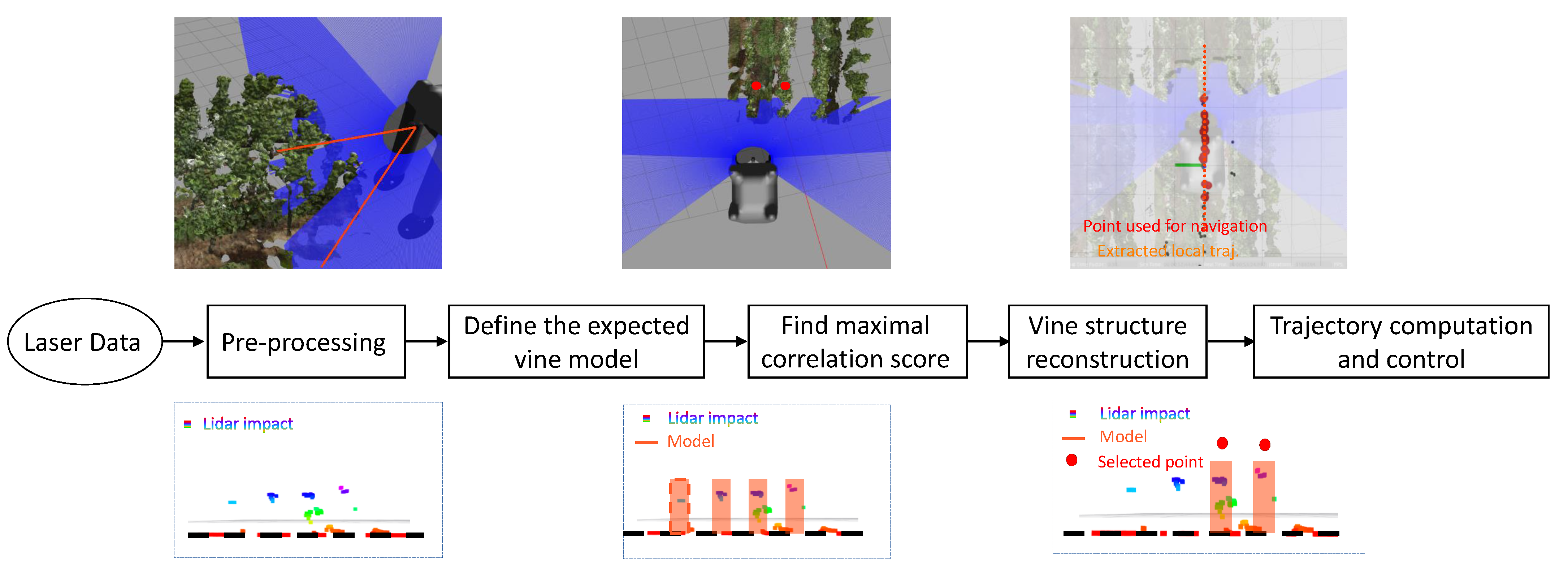
Figure 2.
TRAXX Robot and LiDAR positioning.

Figure 3.
Example of result of the ground inclination compensation in the LiDAR 2D point cloud framework.
Figure 3.
Example of result of the ground inclination compensation in the LiDAR 2D point cloud framework.

Figure 4.
Vine Model Definition in LiDAR framework. (a) Vineyard in Gazebo; (b) LiDAR measurements and corresponding vine model.
Figure 4.
Vine Model Definition in LiDAR framework. (a) Vineyard in Gazebo; (b) LiDAR measurements and corresponding vine model.

Figure 5.
Results of correlation computation and corresponding maximum value. (a) Correlation computation and maximum score; (b) Detection point in the LiDAR framework.
Figure 5.
Results of correlation computation and corresponding maximum value. (a) Correlation computation and maximum score; (b) Detection point in the LiDAR framework.

Figure 6.
Aggregated set-points along the row structure and linear approximation of the selected detecions.
Figure 6.
Aggregated set-points along the row structure and linear approximation of the selected detecions.

Figure 7.
Extended kinematic model of the robot with respect to the reference trajectory . (a) Robot Modeling for control strategy 1; (b) Robot Modeling for control strategy 2.
Figure 7.
Extended kinematic model of the robot with respect to the reference trajectory . (a) Robot Modeling for control strategy 1; (b) Robot Modeling for control strategy 2.

Figure 8.
Illustrations of the summer and winter vineyard. (a) Picture of the summer vineyard; (b) Digitized summer vineyard; (c) Picture of the winter vineyard; (d) Digitized winter vineyard.
Figure 8.
Illustrations of the summer and winter vineyard. (a) Picture of the summer vineyard; (b) Digitized summer vineyard; (c) Picture of the winter vineyard; (d) Digitized winter vineyard.

Figure 9.
Snapshots of the simulation in the summer vineyard. The simulation videos for both strategies are available at this link: https://shorturl.at/iOQ25 (accessed on 22 September 2022).
Figure 9.
Snapshots of the simulation in the summer vineyard. The simulation videos for both strategies are available at this link: https://shorturl.at/iOQ25 (accessed on 22 September 2022).

Figure 10.
Results of the control strategy 1 (top side of the figure) and 2 (bottom side of the figure) on the summer vineyard. (a) Lateral deviation results; (b) Angular deviation results; (c) Front and rear steering angles.
Figure 10.
Results of the control strategy 1 (top side of the figure) and 2 (bottom side of the figure) on the summer vineyard. (a) Lateral deviation results; (b) Angular deviation results; (c) Front and rear steering angles.

Figure 11.
Comparison of angular errors for both control strategies in a summer vineyard.

Figure 12.
Comparison of tracking errors and steering angles with and without the use of rear steering angle. (a) Lateral deviation results; (b) Angular deviation results; (c) Steering angle results.
Figure 12.
Comparison of tracking errors and steering angles with and without the use of rear steering angle. (a) Lateral deviation results; (b) Angular deviation results; (c) Steering angle results.

Figure 13.
Snapshots of the simulation in the winter vineyard. The simulation videos for both strategies are available at this link: https://shorturl.at/cfHVW (accessed on 22 September 2022).
Figure 13.
Snapshots of the simulation in the winter vineyard. The simulation videos for both strategies are available at this link: https://shorturl.at/cfHVW (accessed on 22 September 2022).
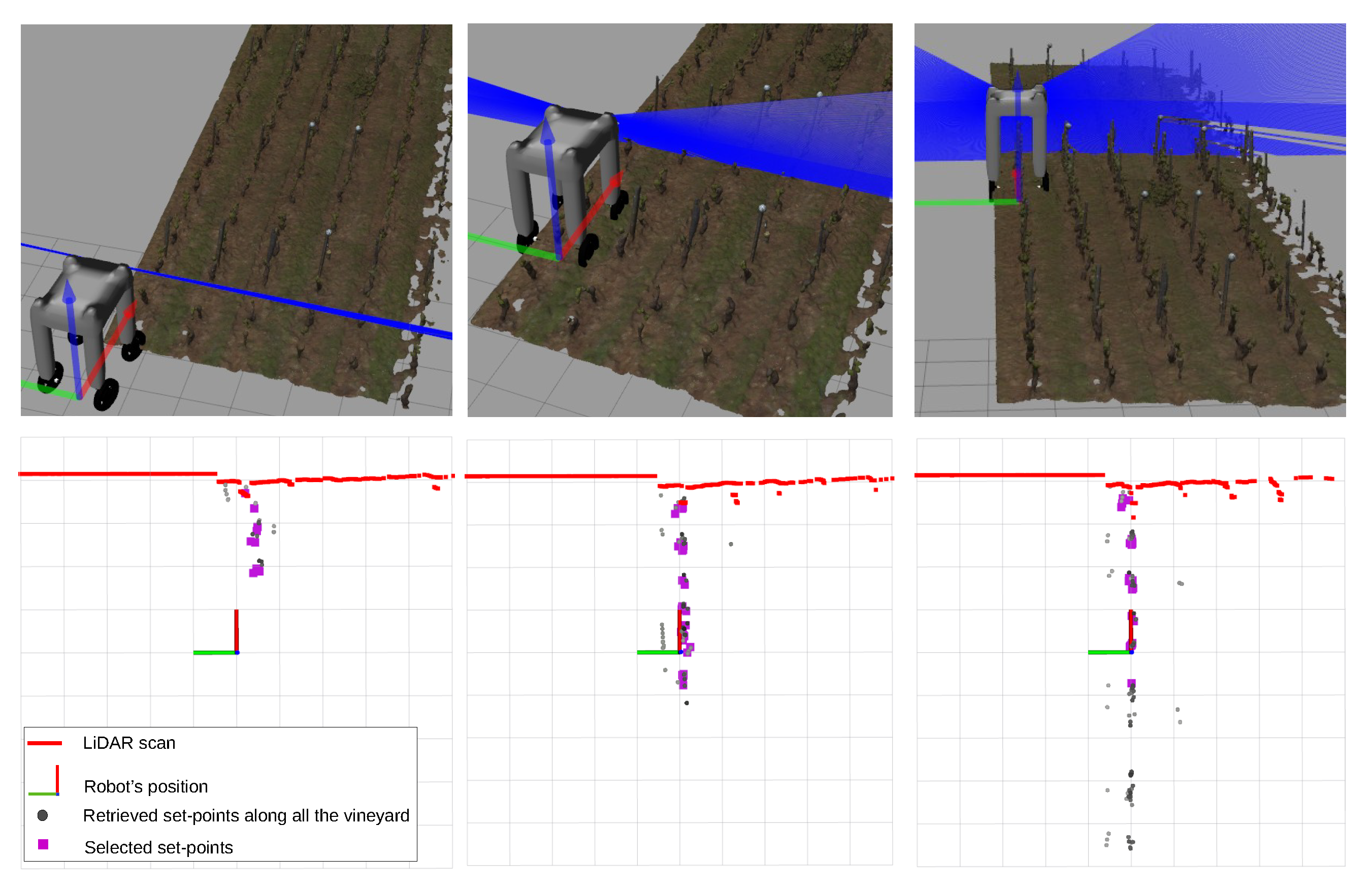
Figure 14.
Results of the control strategy 1 (top side of the figure) and 2 (bottom side of the figure) on the winter vineyard. (a) Lateral deviation results; (b) Angular deviation results; (c) Front and rear steering angles.
Figure 14.
Results of the control strategy 1 (top side of the figure) and 2 (bottom side of the figure) on the winter vineyard. (a) Lateral deviation results; (b) Angular deviation results; (c) Front and rear steering angles.

Figure 15.
Comparison of angular errors for both control strategies in winter vineyard.


Table 1.
The simulation parameters.
| Settings/Scenario | Vine Model Parameters | LiDAR Position | Control Parameters | ||||||
|---|---|---|---|---|---|---|---|---|---|
| Width (Index) | Height (m) | Corr. Threshold | x (m) | y (m) | z (m) | Strategy 1 | Strategy 2 | ||
| Summer Vineyard | 10.0 | 1.0 | 0.25 | 1.0 | 0 | 2.0 | 45 | = −0.9 = 1.0 = 1.0 | = 0.35 = 0.35 |
| Winter Vineyard | 5.0 | 1.0 | 0.25 | 1.0 | 0 | 2.0 | 45 | = −0.9 = 1.0 = 1.0 | = 0.35 = 0.35 |
Publisher’s Note: MDPI stays neutral with regard to jurisdictional claims in published maps and institutional affiliations. |
© 2022 by the authors. Licensee MDPI, Basel, Switzerland. This article is an open access article distributed under the terms and conditions of the Creative Commons Attribution (CC BY) license (https://creativecommons.org/licenses/by/4.0/).
Share and Cite
MDPI and ACS Style
Iberraken, D.; Gaurier, F.; Roux, J.-C.; Chaballier, C.; Lenain, R. Autonomous Vineyard Tracking Using a Four-Wheel-Steering Mobile Robot and a 2D LiDAR. AgriEngineering 2022, 4, 826-846. https://doi.org/10.3390/agriengineering4040053
AMA Style
Iberraken D, Gaurier F, Roux J-C, Chaballier C, Lenain R. Autonomous Vineyard Tracking Using a Four-Wheel-Steering Mobile Robot and a 2D LiDAR. AgriEngineering. 2022; 4(4):826-846. https://doi.org/10.3390/agriengineering4040053
Chicago/Turabian StyleIberraken, Dimia, Florian Gaurier, Jean-Christophe Roux, Colin Chaballier, and Roland Lenain. 2022. "Autonomous Vineyard Tracking Using a Four-Wheel-Steering Mobile Robot and a 2D LiDAR" AgriEngineering 4, no. 4: 826-846. https://doi.org/10.3390/agriengineering4040053