Assessment of RGB Vegetation Indices to Estimate Chlorophyll Content in Sugar Beet Leaves in the Final Cultivation Stage

Abstract

Estimation of chlorophyll content with portable meters is an easy way to quantify crop nitrogen status in sugar beet leaves. In this work, an alternative for chlorophyll content estimation using RGB-only vegetation indices has been explored. In a first step, pictures of spring-sown ‘Fernanda KWS’ variety sugar beet leaves taken with a commercial camera were used to calculate 25 RGB indices reported in the literature and to obtain 9 new indices through principal component analysis (PCA) and stepwise linear regression (SLR) techniques. The performance of the 34 indices was examined in order to evaluate their ability to estimate chlorophyll content and chlorophyll degradation in the leaves under different natural light conditions along 4 days of the canopy senescence period. Two of the new proposed RGB indices were found to improve the already good performance of the indices reported in the literature, particularly for leaves featuring low chlorophyll contents. The 4 best indices were finally tested in field conditions, using unmanned aerial vehicle (UAV)-taken photographs of a sugar beet plot, finding a reasonably good agreement with chlorophyll-meter data for all indices, in particular for I₂ and (R−B)/(R+G+B). Consequently, the suggested RGB indices may hold promise for inexpensive chlorophyll estimation in sugar beet leaves during the harvest time, although a direct relationship with nitrogen status still needs to be validated.

1. Introduction

In sugar beet (Beta vulgaris L.), nitrogen plays a major role in the spreading of leaves to capture sunlight. It is considered a decisive factor in the growth rate of both leaves and the storage root [1]. Nitrogen concentration in leaves increases in the first 70 days of the sugar beet’s growth cycle, and then decreases as the growth cycle progresses [2]. It is known that leaf chlorophyll content is related to N status [3], and a decrease in chlorophyll content and an acceleration of canopy senescence towards the end of the crop cycle is often reported [4]. Low levels of N result in a pale green foliage due to low chlorophyll concentration [5], although late N application increases chlorophyll concentration in leaves [6].

The determination of leaf N levels in the last stage of sugar beet’s growth cycle becomes relevant since it has been demonstrated that late N incorporations or releases from the soil decrease sucrose content [7]. Draycott et al. [5] and Malnou et al. [6] showed that, beyond an optimum level, N has a negative effect on sugar yield. Soils that release a lot of N late in the summer feature lower yields, given that polarization (i.e., the apparent sucrose content) in that growth stage develops inversely to N availability. Gordo-Ingelmo [2] reported that sugar beet reacts to N fertilization increases with a larger development of leaves and roots, which in turn cause an excessive use of sucrose and an increase of nonsugars. This mainly happens in cases of excessive organic fertilization, because part of the N is released belatedly, causing a stop of root ripeness.

This crucial importance of N to multiple aspects of sugar beet growth (and other crops) has led to the development of different methods to determine N levels, including destructive chemical analyses [8], subjective leaf color charts, fluorescence techniques (including the fluorescence excitation ratio method [9], fluorescence spectral records [10] and fluorescence kinetic records [11]) and chlorophyll monitoring methods [12,13,14]. Most of the fluorescence-based techniques either require costly instrumentation or are labor-intensive, in a similar way as chlorophyll meter use. In spite of this drawback, measurements conducted with chlorophyll meters have proven to be highly correlated with chemical analyses in the case of sugar beet [6,15].

Another accepted method for N estimation is based on the use of remote sensing image analysis [16,17]. In this technique, images captured at different scales with different types of sensors are used to calculate vegetation indices. These indices allow leaf chlorophyll content evaluation [18], yield prediction [19,20,21], nutrient status estimation [22,23], disease [24,25] and weed detection [26,27], crop management [28] or crop growth monitoring [29].

Vegetation indices based on narrow-band imaging spectrometers (also called hyperspectral sensors) have been proposed, which—in the case of sugar beet—have been shown to have great potential to remotely estimate LAI and canopy chlorophyll content (RMSE ≤ 10%) and to retrieve canopy nitrogen content (RMSE = 10%) [30]. Nonetheless, they remain expensive and create very large data volumes [31], while farmers require short-term, low-expense solutions to manage their fields. To comply with these requirements, Kawashima et al. [32] put forward a facile and low-cost diagnostic method to assess the nutrient status of plants based on the estimation of chlorophyll content of wheat and rye leaves, using a portable color video camera and a personal computer. The authors showed that leaf chlorophyll content could be estimated with sufficient accuracy using basic equipment. This research line has been continued in recent years, with the proposal of indices calculated from RGB bands of the visible light spectrum, using inexpensive, off-the-shelf cameras [12,31,33,34,35].

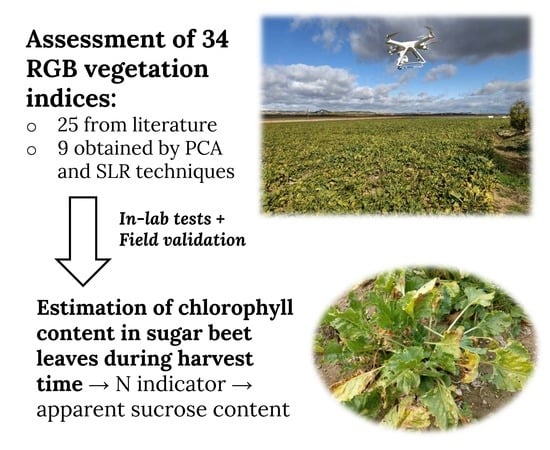
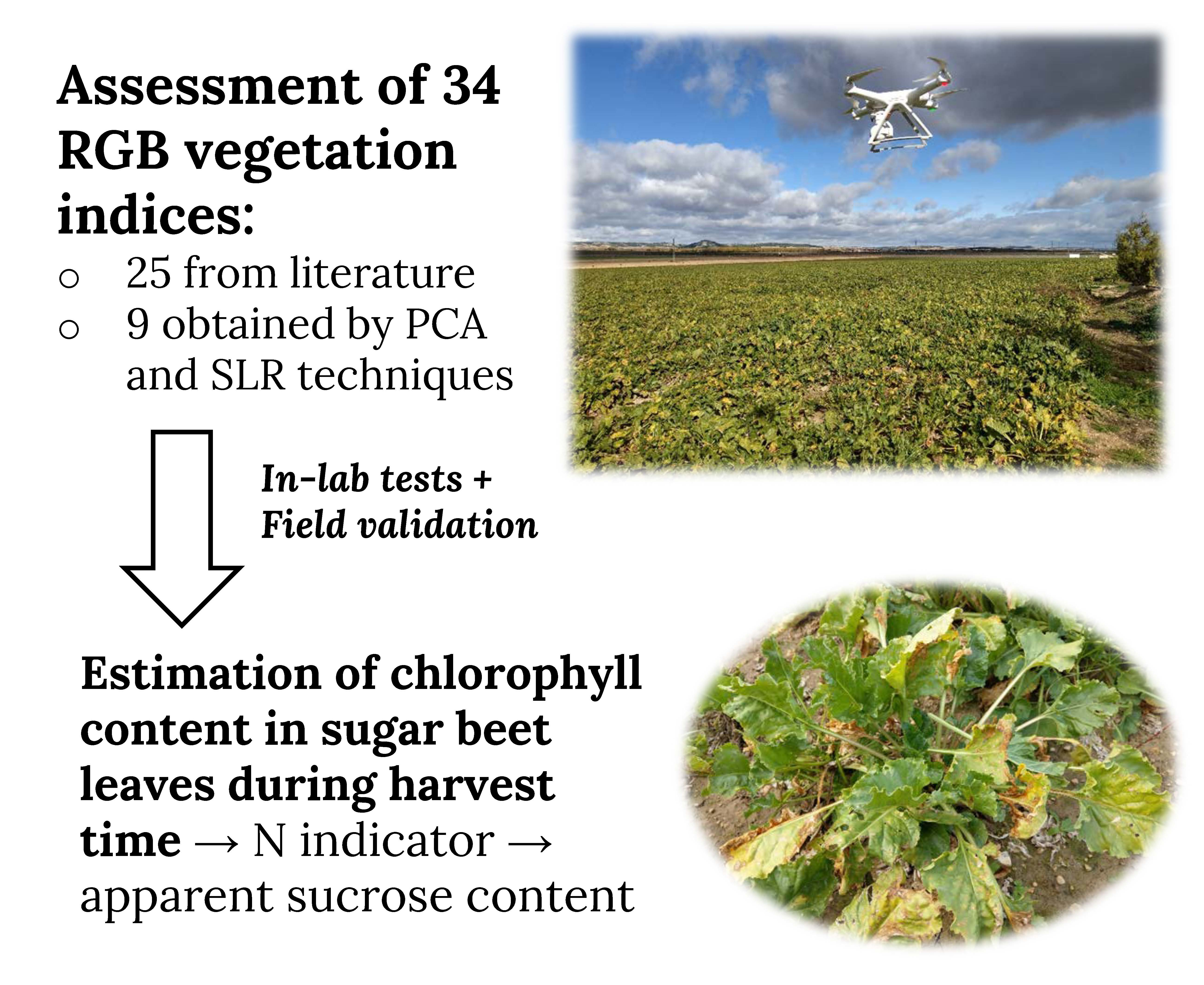
In line with aforementioned studies, the aim of the research presented herein was to verify the validity of such methodologies based on index calculation from the RGB bands of leaf images (obtained using a non-scientific-grade camera) for chlorophyll content evaluation in sugar beet leaves during the final growth stage. For this validation, in a first step, different size and color sugar beet leaves from commercial farms were collected and photographed in the laboratory, extracting RGB values. Twenty-five indices proposed in the literature were tested, and nine novel indices were proposed. In a second step, the best indices were tested in field conditions, comparing conventional chlorophyll-meter measurements with the values estimated using UAV-taken photographs of a sugar beet plot.

2. Materials and Methods

2.1. Sampling Site and Crop Management

The experiment was conducted during the sugar beet harvest season, from 18 October, 2018 until 21 October, 2018. Solar radiation conditions during the experiment (13.87, 11.29, 11.32 and 6.65 MJ·m⁻² on days 1 to 4, respectively) were obtained from an automatic weather station belonging to the SIAR (Agroclimatic Information System for Irrigation) network of the Spanish Ministry of Agriculture, Food and Environment. The leaves were taken from a commercial plantation located in Magaz de Pisuerga (41°58′1.2″N, 4°26′44.2″W, altitude 740 m.a.s.l.). A description of the experimental site is provided in previous work [36]. The sowing, delayed due to an unusually long rainfall period, was conducted on 16 April, 2018. The average population density was 125,000 plants·ha⁻¹ (considering a sowing distance of 13.7 cm and a seedling emergence of 86%). Crop management practices strictly followed the Spanish Research Association for Sugar Beet Crop Improvement (AIMCRA)’s recommendations, described in [37]. The irrigation dose was 460 mm.

Five plants of ‘Fernanda KWS’ variety were randomly selected and brought to the laboratory within 40 min.

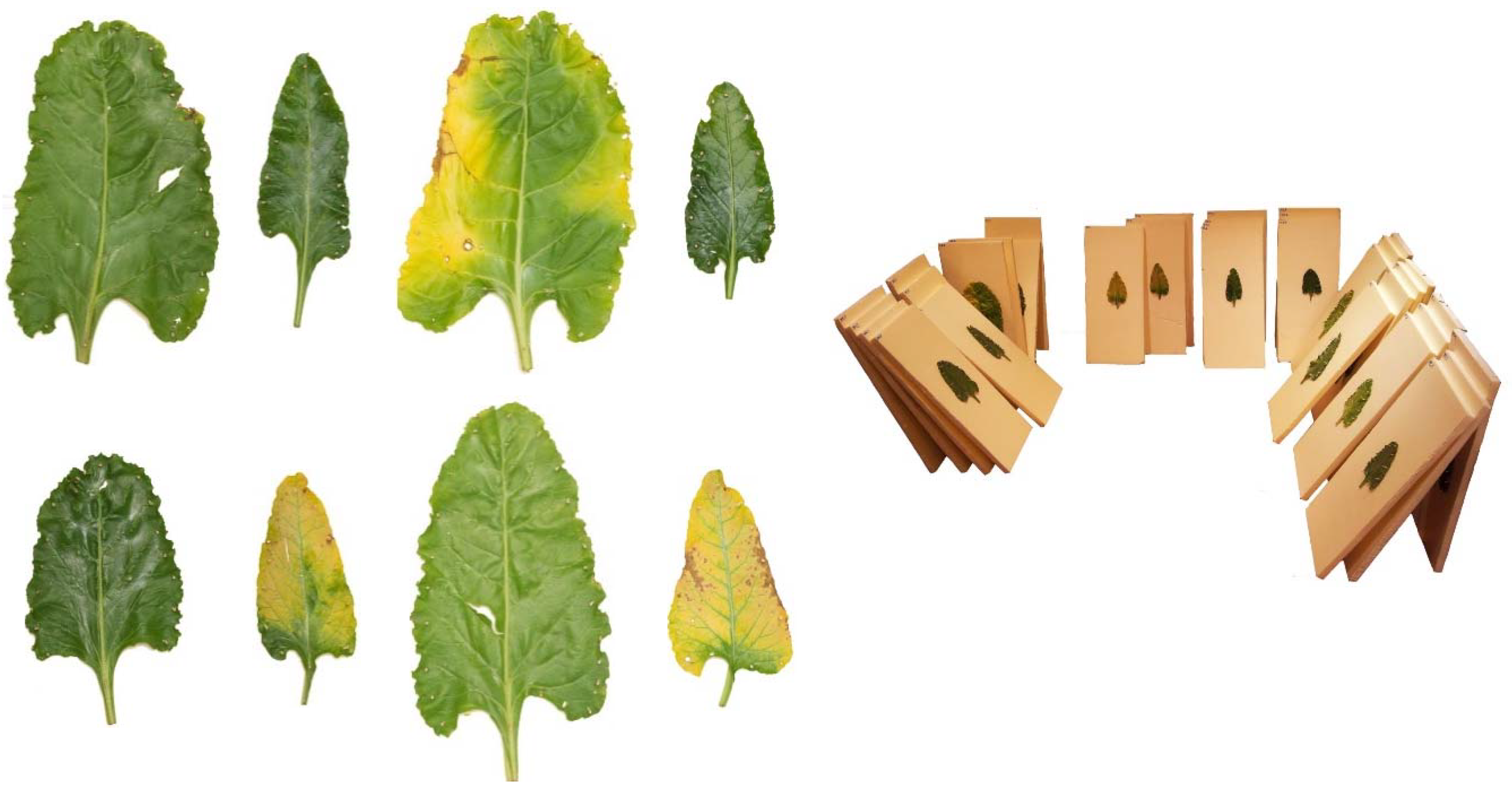
Once at the laboratory, seven leaves were randomly selected from each plant in order to obtain a representative sample in terms of sizes and colorings. Figure 1 (left) shows some of the leaves used in the experiment.

2.2. Chlorophyll Measurements

For each leaf, 10 instant and nondestructive measurements, with an area of 0.71 cm², were taken using a CCM-200 plus (Opti-Sciences; Hudson, NH, USA) optic chlorophyll meter. This apparatus measures the absorbance at λ = 653 nm and λ = 931 nm and calculates a chlorophyll concentration index (CCI) value that is proportional to the amount of chlorophyll in the sample. The average of the 10 measurements was considered as the chlorophyll content in the leaf at each moment.

2.3. RGB Data Acquisition

Each leaf was vertically and independently placed on a 50 × 30 cm polyurethane sheet (Figure 1, right), and pictures were taken during 4 days at different times (at 11:00, 13:30 and 17:00 on 18 October; at 10:00 on 19 October and 20 October; and at 10:00, 14:00 and 16:00 on 21 October) in a laboratory room, using only natural light coming from a single north-facing window covered with a thin translucent curtain. Photographs were taken in vertical position with a Sony α55 (SLT-A55V, Sony, Tokyo, Japan) camera with an APS-CCMOS sensor of 16.2 MPx resolution and a Sony SAL 55-200 mm lens. The camera was mounted on a tripod in a fixed position (1 m height and 2.5 m far from the leaf). Every picture was taken with 4912 × 3264 pixels resolution, 55 mm focal distance, ISO-1600 sensitivity setting, using the aperture-priority mode with white balance set to manual and punctual measurement of exposition. Before each photograph was taken, a grey/white Lastolite Ezybalance card (Manfrotto, Cassola, Italy) was placed in front of the leaf to be photographed and used for exposure and color correction. It should be clarified that Ezybalance works as a reflectance standard of 18% of brightness [38].

2.4. Image Processing and Color Indices Calculation

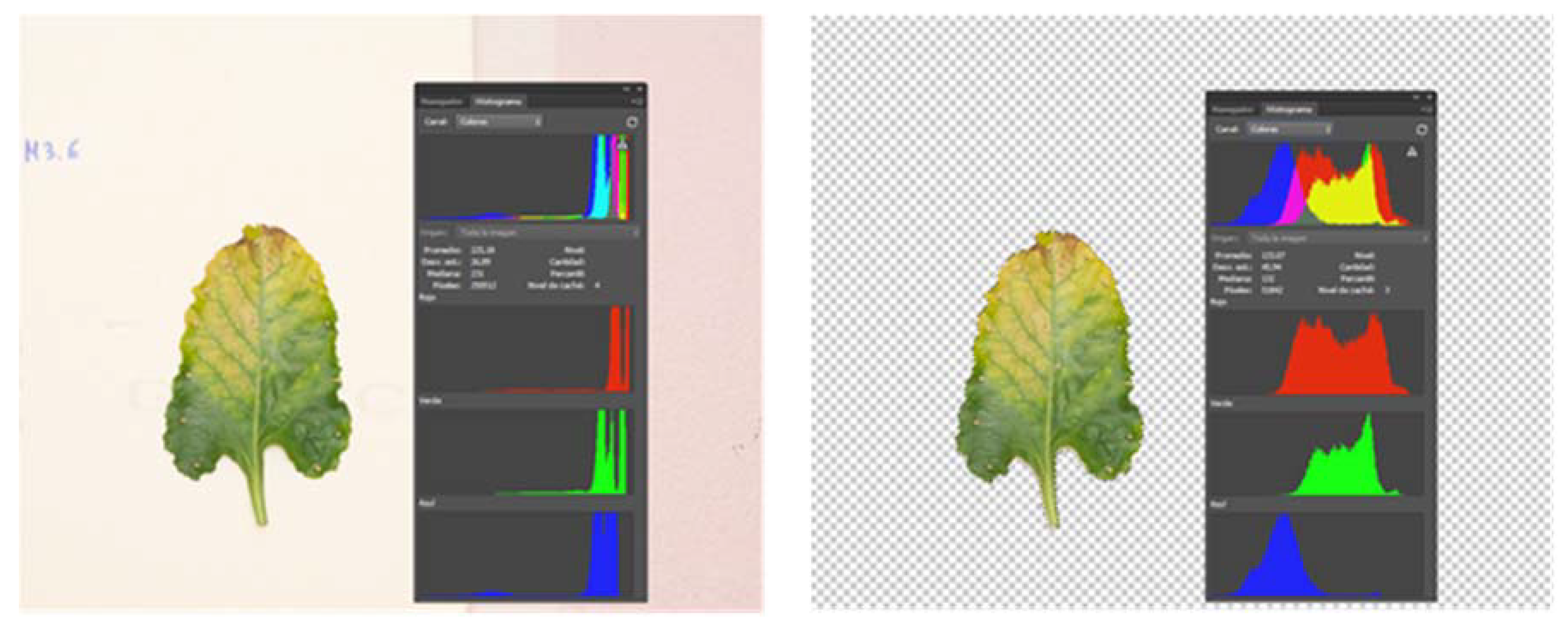
Photographs were saved in ARW format, and were analyzed using Adobe Photoshop v.14.1 (Adobe Systems Inc., San Jose, CA, USA). Besides RGB levels, this software offers a channel for the brightness scale in the histogram tool. A routine was designed to remove the background of each photograph, using several functionalities of the program to keep only the leaf pixels. The average RGB value for the total surface of each leaf was calculated by means of the histogram tool (Figure 2). Accordingly, each leaf presented specific RGB coordinates per shoot, based on which the different color indices were calculated.

Pictures were analyzed according to three main groups of vegetation indices: indices reported in the literature (subdivided into those previously studied by Kawashima et al. [32] and those from other sources), new indices obtained by means of stepwise linear regression (SLR) and new indices obtained by principal component analysis (PCA) (

Table 1. List of the color vegetation indices considered in study, including their equations and sources.

Index	Definition	Reference
R	red (0–255)	[32]
G	green (0–255)	[32]
B	blue (0–255)	[32]
r	R/(R+G+B)	[32]
g	G/(R+G+B)	[32]
b	B/(R+G+B)	[32]
R−G		[32]
R−B		[32]
G−B		[32]
(R−G)/(R+G)		[32,39]
(R−B)/(R+B)		[32]
(G−B)/(G+B)		[32]
(R−G)/(R+G+B)		[26,32]
(R−B)/(R+G+B)		[32]
(G−B)/(R+G+B)		[26,32]
RGRI	R/G	[12]
GLI	(2G−R−B)/(2G+R+B)	[40]
VARI	(G−R)/(G+R−B)	[41]
IPCA	0.994|R−B| + 0.961|G−B| + 0.914|G−R|	[12]
ExR	1.4r − g	[42,43]
ExB	1.4b − g	[43]
ExG	2g – r − b	[26,43]
ExGR	ExG − ExR	[42,43]
Gray	0.2898r + 0.5870g + 0.1140b	[44]
CIVE	0.441r − 0.811g + 0.385b + 18.78	[45]
PCA1	−0.977b + 0.916((G−B)/(G+B)) + 0.995((R−B)/(R+B)) + 0.771 ((R−G)/(R+G))	This work
PCA2	0.999|R−B| + 0.92|G−B| + 0.886|R−G|	This work
I1	R + G − 2B	This work
SLR1	−60430 − 0.7316B + 69680b + 112800g + 28270((G−B)/(G+B)) − 23890((R−B)/(R+B)) + 68380((R−G)/(R+G))	This work
SLR2	−46240 − 2.678B + 1.05G + 52570b + 87420g + 20720((G−B)/(G+B)) − 18240((R−B)/(R+B)) + 52500((R−G)/(R+G))	This work
SLR3	−25373 + 30106b + 46539g + 12776((G−B)/(G+B)) − 10507((R−B)/(R+B)) + 28821((R−G)/(R+G))	This work
SLR4	−44312 + 51689b + 81995g + 21751((G−B)/(G+B)) − 18156((R−B)/(R+B)) + 50425((R−G)/(R+G))	This work
SLR5	−41048 + 46964b + 76841g + 19998((G−B)/(G+B)) − 17173((R−B)/(R+B)) + 47162((R−G)/(R+G))	This work
I2	0.55 + 11.4((G−B)/(G+B)) − 12.5((R−B)/(R+B)) + 9((R−G)/(R+G))	This work

). The indices were calculated for different datasets: for each shoot, for all the shoots taken on the same day and for the mean of daily shoots. They were also calculated for three global datasets: for all the eight shoots together, for the means of all days and, finally, for the mean of the darkest shoot (18 October 2018, 17:00) and for the brightest one (21 October 2018, 14:00). Besides this, the entire dataset was divided into two subdatasets for validation purposes, as discussed below.

New Indices and Validation

In order to explore the possibility of obtaining new indices, PCA and SLR methodologies were used. In a previous step, to ensure an appropriate validation of the calculated indices, the dataset was divided into two subdatasets, the first one was used to generate the parameters of the new indices and the second one was used to estimate the statistical error. Subdatasets were defined by choosing shoots alternately. Thus, the first subdataset included shoots #1 and #3 from 18 October, shoot #1 from 20 October and shoot #2 from 21 October; the second subdataset consisted of photographs from shoot #2 from 18 October, shoot #1 from 19 October, and shoots #1 and #3 from 21 October.

PCA indices: PCA multivariate procedure was conducted with IBM SPSS Statics 21 (IBM Corp., Armonk, NY, USA). PCA1 and PCA2 indices (Table 1) were obtained as the values of eigenvectors associated with the highest eigenvalues, i.e., the principal components (PC₁) of the datasets, which explained the largest amount of variance in the data, according to the procedure described by Saberioon et al. [12]. Results from the PCA analysis for PCA1 and PCA2 are presented in the supporting information file. I₁ index was derived from the other PCA indices.

SLR indices: the SLR functionality in R software (v.2.15.3, R Development Core Team, Vienna, Austria [46]) was used as an alternative procedure to obtain new indices. Some literature indices were considered as inputs, and resultant indices were calculated by adding and removing variables one by one [44], using AIC (Akaike Information Criterion) method for variable selection [47]. Indices SLR1 to SLR5 and I₂ (Table 1) were obtained using this procedure.

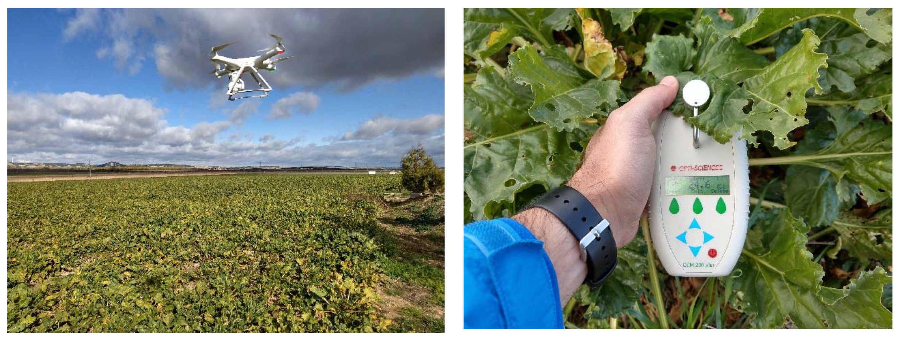
2.5. Field Test

After the in-lab assessment of the 34 RGB indices, the 4 vegetation indices for which the best performance was found were tested in real field conditions, in a sugar beet plot located in Soto de Cerrato, Palencia, Spain (41°56′23″N, 4°26′78″W, altitude 730 m.a.s.l.) on 8 November, 2019. Images were captured with a low-cost Xiaomi Mi Drone (1080P version), with f/2.6 aperture and a 1/2.3 inches CMOS sensor (Figure 3, left).

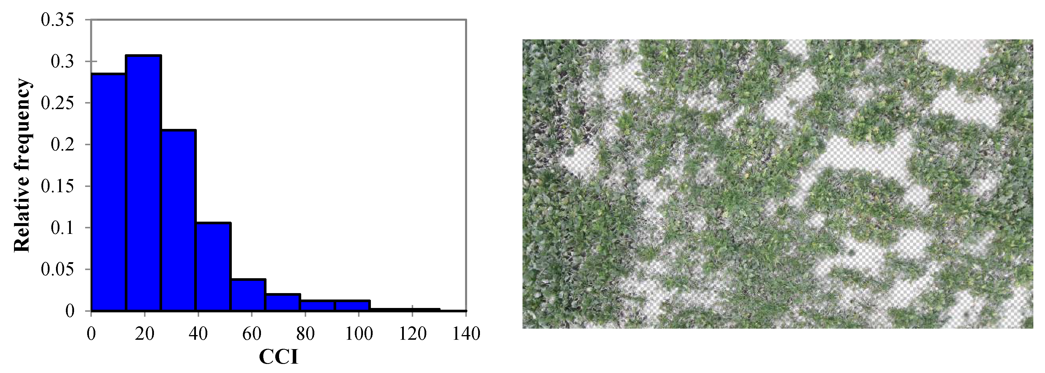
The soil was removed using Adobe Photoshop (in a similar fashion to the background removal in the in-lab photographs), and average RGB values of photographs taken at different heights were used for the calculation of the indices.

For comparison purposes, 500 chlorophyll measurements were randomly conducted in the same sugar beet plot with the CCM-200 plus chlorophyll meter (Figure 3, right).

2.6. Statistical Analysis

STATISTICA v. 8.0 (TIBCO, Palo Alto, CA, USA) was used for descriptive analysis, including maximum, minimum, mean, standard error and coefficients of variation (CV) of the different chlorophyll concentrations and for all the indices. Correlation matrices—with Pearson correlation coefficients (R) and p-values for each index—were also calculated for each shoot, for all the shoots in a day, for the mean of daily shoots and, finally, for three global subdatasets (i.e., for all the eight shoots together, for the means of each day together, and for the means of one shoot of the first day and one shoot of the last day).

Graphs to allow comparisons between different indices and chlorophyll concentrations were also plotted, including regression equations and coefficients of determination (R²).

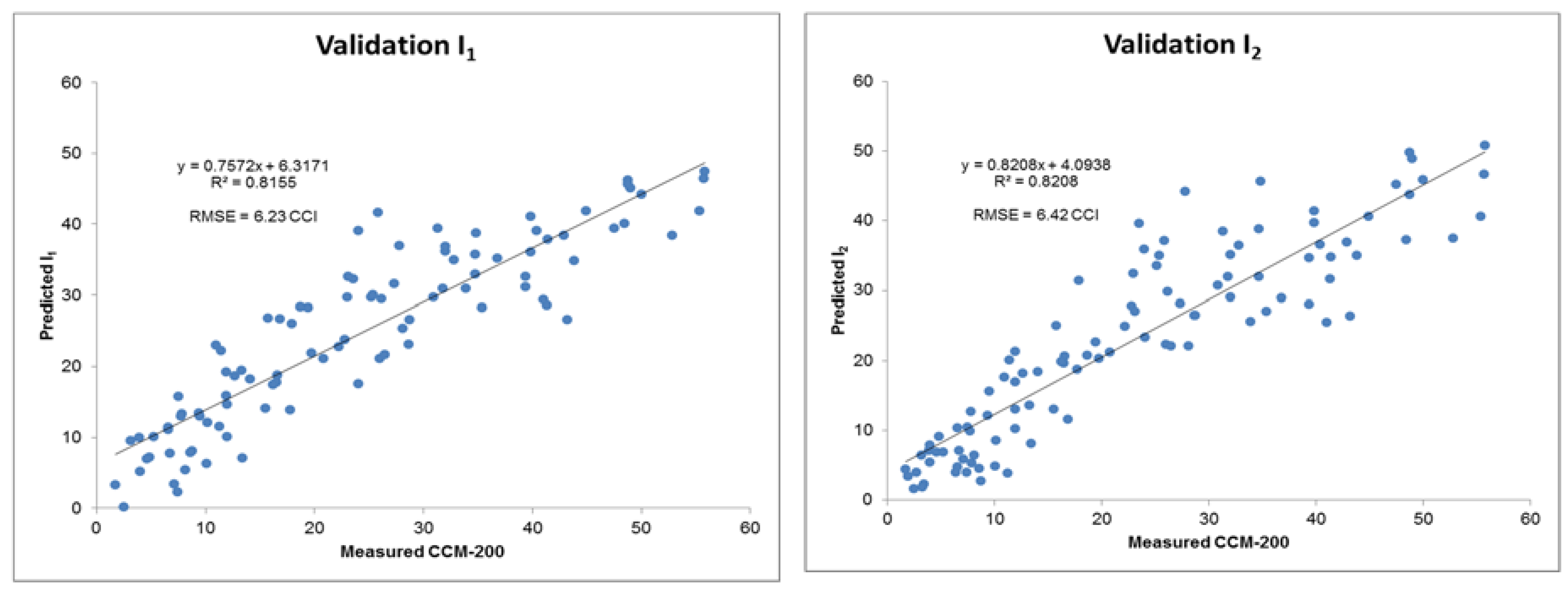
For validation of the new indices, the root-mean-square error (RMSE) was calculated as follows:

$$\mathrm{RMSE}=\sqrt{\frac{1}{\mathrm{n}}{\displaystyle \sum }_{\mathrm{i}=1}^{\mathrm{n}}{\left(\mathrm{Mi}-\mathrm{Pi}\right)}^2}$$

(1)

where M_i = measurement with CCM-200, P_i = predicted by index, and n = number of observations. Units are CCI.

3. Results and Discussion

3.1. Chlorophyll Content Measurements

From the summary of descriptive statistics for the CCM-200 measurements shown in

Table 2. Summary of descriptive statistics for chlorophyll measurements: minimum, maximum, mean, standard error and coefficient of variation (CV).

Day	Min	Max	Mean	Std. Error	CV
1	2.76	55.82	24.49	2.55	61.60
2	2.51	55.71	23.37	2.52	63.91
3	2.00	55.48	21.78	2.64	71.80
4	1.74	55.36	21.07	2.73	75.57
Overall	1.74	55.82	22.57	1.29	67.74

, one can see how chlorophyll content decreased over time, evidencing chlorophyll deterioration in the leaves as time went by. The high values of the coefficient of variation (CV) would be due to the heterogeneity of the samples, since diverse coloring and a wide size range were purposefully part of the sampling process. This fact was also evidenced in the calculated vegetation indices (Table S1), which showed a wide variance of coefficients because of the heterogeneity of the samples.

3.2. Correlation of Chlorophyll Measurements and Color Indices

Pearson correlation coefficients for each index are discussed according to previously defined groups of indices. It is worth noting that indices with high R values were found in all the groups, which in good agreement with other studies in the literature that found close correlations between chlorophyll content and RGB values, e.g., for potato and soybean leaves [34,48].

3.2.1. Indices Studied by Kawashima and Nakatani

The results obtained for this group of indices (

Table 3. Correlation coefficients for indices studied by Kawashima et al. [32]. Results are given for each individual shoot, for daily values on days #1 and #4 (taking into account the three shoots altogether or the mean values of the three shoots) and for global datasets. The latter include data from all the days using the eight shoots, data from all the days using mean values for days #1 and #4 and mean values between extreme shoots (the darkest shoot from day #1 and the brightest shoot from day #4). The highest R-values are highlighted in bold typeface. Significance levels: ** (p < 0.01) and * (p < 0.05).

Index	Day 1					Day 2	Day 3	Day 4					Global
	Shoot 1	Shoot 2	Shoot 3	3 Shoots Together	Mean of Shoots	Shoot 1	Shoot 1	Shoot 1	Shoot 2	Shoot 3	3 Shoots Together	Mean of Shoots	8 Shoots Together	Means of Shoots	Extreme Shoots
R	−0.8357 **	−0.8079 **	−0.8156 **	−0.818 **	−0.8705 **	−0.8215 **	−0.7431 **	−0.8532 **	−0.8536 **	−0.9213 **	−0.8613 **	−0.9094 **	−0.798 **	−0.8449 **	−0.7632 **
G	−0.8161 **	−0.7823 **	−0.8011 **	−0.7969 **	−0.9038 **	−0.7662 **	−0.6498 **	−0.7764 **	−0.7366 **	−0.8744 **	−0.7621 **	−0.8815 **	−0.7411 **	−0.8471 **	−0.6947 **
B	0.2616 ns	0.349 *	0.2934 ns	0.2981 **	0.4271 **	0.0835 ns	−0.0296 ns	−0.119 ns	−0.0249 ns	−0.4242 *	−0.1592 ns	−0.2232 ns	−0.0036 ns	0.0079 ns	0.086 **
r	−0.9019 **	−0.9007 **	−0.8904 **	−0.897 **	−0.8969 **	−0.8915 **	−0.8678 **	−0.9024 **	−0.904 **	−0.9062 **	−0.8986 **	−0.9086 **	−0.8786 **	−0.8824 **	−0.8788 **
g	−0.4695 ns	−0.4684 ns	−0.4589 **	−0.4632 **	−0.4771 **	−0.084 ns	0.1786 ns	0.4043 **	0.4538 **	0.507 **	0.4528 **	0.4651 **	0.0611 ns	0.0539 ns	0.0501 **
b	0.9243 **	0.9151 **	0.9091 **	0.914 **	0.9205 **	0.8997 **	0.8463 **	0.864 **	0.8241 **	0.8597 **	0.8325 **	0.868 **	0.8535 **	0.8696 **	0.8496 **
R-G	−0.6707 **	−0.6682 **	−0.6603 **	−0.6662 **	−0.6645 **	−0.749 **	−0.7179 **	−0.7934 *	−0.8142 **	−0.8 **	−0.8016 **	−0.8036 **	−0.7227 **	−0.7186 **	−0.7236 **
R-B	−0.9102 **	−0.9156 **	−0.8963 **	−0.9071 **	−0.9114 **	−0.8879 **	−0.8648 **	−0.9186 **	−0.9188 **	−0.932 **	−0.918 **	−0.9289 **	−0.8879 **	−0.8977 **	−0.8802 **
G-B	−0.9151 **	−0.9332 **	−0.9082 **	−0.9183 **	−0.931 **	−0.8824 **	−0.8506 **	−0.9043 **	−0.8381 **	−0.8813 **	−0.8639 **	−0.8905 **	−0.8678 **	−0.8858 **	−0.8527 **
(R-G)/(R+G)	−0.7399 **	−0.7353 **	−0.7341 **	−0.7362 **	−0.7359 **	−0.8034 **	−0.7632 **	−0.8376 **	−0.8437 **	−0.8482 **	−0.8418 **	−0.8449 **	−0.7666 **	−0.7609 **	−0.7549 **
(R-B)/(R+B)	−0.9276 **	−0.9201 **	−0.9123 **	−0.9183 **	−0.9226 **	−0.9068 **	−0.8752 **	−0.9004 **	−0.8823 **	−0.9037 **	−0.8827 **	−0.9081 **	−0.8813 **	−0.8941 **	−0.8809 **
(G-B)/(G+B)	−0.9034 **	−0.8891 **	−0.8849 **	−0.8895 **	−0.8996 **	−0.8699 **	−0.7511 **	−0.7438 **	−0.6626 **	−0.7164 **	−0.6888 **	−0.7334 **	−0.7766 **	−0.7957 **	−0.765 **
(R-G)/(R+G+B)	−0.7167 **	−0.711 **	−0.7096 **	−0.7122 **	−0.7118 **	−0.7899 **	−0.753 **	−0.8297 **	−0.8369 **	−0.8409 **	−0.8344 **	−0.8377 **	−0.7549 **	−0.7492 **	−0.7435 **
(R-B)/(R+G+B)	−0.9288 **	−0.9238 **	−0.9151 **	−0.9212 **	−0.9241 **	−0.909 **	−0.8845 **	−0.9088 **	−0.8981 **	−0.9125 **	−0.8958 **	−0.9165 **	−0.8908 **	−0.9015 **	−0.8916 **
(G-B)/(R+G+B)	−0.8748 **	−0.8604 **	−0.8584 **	−0.8614 **	−0.8733 **	−0.8223 **	−0.6454 **	−0.6046 **	−0.4875 **	−0.5178 **	−0.5206 **	−0.5603 **	−0.6894 **	−0.7075 **	−0.6753 **

ns: not significant

) were consistent with the findings of Kawashima et al. [32]. (G−B) and (R−B) (i.e., the corrected values for R and G based on B) showed several of the highest correlation values in different shoots, although (R−B)/(R+G+B) was the index with the highest overall values, performing better when the eight shoots were analyzed, for the average of the first and the last day, or of the two shoots with the greatest difference in brightness. Actually, (G−B) showed high correlation values (above 0.90) in measurements conducted on day #1 but showed a rather irregular behavior on the rest of days. On the other hand, (R−B) showed a more regular behavior, although its correlation indices decreased when global data were analyzed. The higher correlation coefficients for (R−B) and (G−B) than for R and G alone may be explained because taking B as the base value decreases the bias noise in R, G and B, as noted by [12,32].

In this experiment, (R−B)/(R+G+B) would have a similar role to that of (R−B)/(R+B) in [32], which is consistent with the fact that both indices, in both studies, have very close results in their correlation indices with chlorophyll content (see Figure S1).

3.2.2. Indices from Other Sources

In this group, it could be observed how the I_PCA index developed by Saberioon et al. [12] attained the best results (

Table 4. Correlation coefficients for indices studied for different researchers. Results are given for each individual shoot, for daily values on days #1 and #4 (taking into account the three shoots altogether or the mean values of the three shoots) and for global datasets. The latter include data from all the days using the eight shoots, data from all the days using mean values for days #1 and #4 and mean values between extreme shoots (the darkest shoot from day #1 and the brightest shoot from day #4). The highest R-values are highlighted in bold typeface. Significance levels: ** (p < 0.01) and * (p < 0.05).

Index	Day 1					Day 2	Day 3	Day 4					Global
	Shoot 1	Shoot 2	Shoot 3	3 Shoots Together	Mean of Shoots	Shoot 1	Shoot 1	Shoot 1	Shoot 2	Shoot 3	3 Shoots Together	Mean of Shoots	8 Shoots Together	Means of Shoots	Extreme Shoots
RGRI	−0.7385 **	−0.7324 **	−0.732 **	−0.7341 **	−0.733 **	−0.7981 **	−0.7576 **	−0.8288 **	−0.8356 **	−0.8377 **	−0.8325 **	−0.8358 **	−0.7619 **	−0.7563 **	−0.7514 **
GLI	−0.4712 *	−0.47 **	−0.4598 **	−0.4647 **	−0.4788 **	−0.0836 ns	0.1829 ns	0.4074 *	0.4564 **	0.5089 **	0.4553 **	0.465 **	0.0646 ns	0.0563 ns	0.0541 **
VARI	0.781 **	0.7776 **	0.776 **	0.7781 **	0.7772 **	0.8261 **	0.7806 **	0.851 **	0.8549 **	0.8599 **	0.8539 **	0.8569 **	0.7867 **	0.781 **	0.7746 **
IPCA	−0.9205 **	−0.929 **	−0.9058 **	−0.9181 **	−0.928 **	−0.888 **	−0.8607 **	−0.9057 **	−0.9001 **	−0.9165 **	−0.9008 **	−0.9143 **	−0.8907 **	−0.9066 **	−0.8855 **
ExR	−0.7866 **	−0.7842 **	−0.7784 **	−0.7829 **	−0.7814 **	−0.8254 **	−0.7896 **	−0.853 **	−0.8594 **	−0.8611 **	−0.8557 **	−0.86 **	−0.7969 **	−0.7929 **	−0.789 **
ExB	0.8913 **	0.8779 **	0.8751 **	0.8785 **	0.8883 **	0.8497 **	0.7106 **	0.6938 **	0.5945 **	0.6364 **	0.6232 **	0.6642 **	0.7411 **	0.7587 **	0.729 **
ExG	−0.4695 **	−0.4684 **	−0.4589 **	−0.4632 **	−0.4774 **	−0.084 ns	0.1786 ns	0.4043*	0.4538 **	0.507 **	0.4528 **	0.4624 **	0.0611 ns	0.0525 ns	0.0501 **
ExGR	0.233 ns	0.2095 ns	0.2313 ns	0.2236 *	0.2244 *	0.547 **	0.5606 **	0.7027 **	0.7169 **	0.7382 **	0.7184 **	0.7227 **	0.5188 **	0.5093 **	0.4966 **
GREY	−0.8345 **	−0.8189 **	−0.818 **	−0.8204 **	−0.8336 **	−0.7501 **	−0.4969 **	−0.3947 *	−0.2603 ns	−0.2537 ns	−0.294 **	−0.3165 ns	−0.5713 **	−0.5869 **	−0.5921 **
CIVE	0.382 *	0.386 *	0.3732 *	0.3786 *	0.3909 *	−0.0358 ns	−0.253 ns	−0.4693 **	−0.5095 **	−0.5577 **	−0.5101 **	−0.5191 **	−0.145 *	−0.1364 ns	−0.1679 ns

ns: not significant

), behaving in a stable manner throughout all the experiment. RGRI [12], VARI [41] and ExR [42] indices also showed high correlations (above 0.75). These last two indices have been used for vegetation extraction and artificial vision in agriculture [44]. The relationship of ExR and I_PCA with the chlorophyll measurements during the experiment are shown in Figure S2. It may be inferred that I_PCA exhibited a better performance, with higher R² and lower dispersion.

3.2.3. Indices Calculated via PCA

This group included the indices calculated ex novo via PCA. The three new indices (detailed in Table 1) showed a similar behavior to that of I_PCA (see

Table 5. Correlation coefficients for new indices obtained by PCA process. Results are given for each individual shoot, for daily values on days #1 and #4 (taking into account the three shoots altogether or the mean values of the three shoots) and for global datasets. The latter include data from all the days using the eight shoots, data from all the days using mean values for days #1 and #4 and mean values between extreme shoots (the darkest shoot from day #1 and the brightest shoot from day #4). The highest R-values are highlighted in bold typeface. Significance level: ** (p < 0.01).

Index	Day 1					Day 2	Day 3	Day 4					Global
	Shoot 1	Shoot 2	Shoot 3	3 Shoots Together	Mean of Shoots	Shoot 1	Shoot 1	Shoot 1	Shoot 2	Shoot 3	3 Shoots Together	Mean of Shoots	8 Shoots Together	Means of Shoots	Extreme Shoots
PCA1	−0.9277 **	−0.9198 **	−0.912 **	−0.918 **	−0.9227 **	−0.906 **	−0.8703 **	−0.894 **	−0.8724 **	−0.8964 **	−0.8742 **	−0.9015 **	−0.8775 **	−0.8913 **	−0.8768 **
PCA2	−0.9205 **	−0.9289 **	−0.9058 **	−0.918 **	−0.9278 **	−0.8881 **	−0.8608 **	−0.9059 **	−0.9006 **	−0.9168 **	−0.9011 **	−0.9146 **	−0.8908 **	−0.9065 **	−0.8855 **
I1	−0.9183 **	−0.9291 **	−0.9072 **	−0.9178 **	−0.9254 **	−0.892 **	−0.8729 **	−0.929 **	−0.9152 **	−0.9328 **	−0.9183 **	−0.9346 **	−0.8924 **	−0.9061 **	−0.8831 **

). PCA2 used the three bands, as did I_PCA. PCA1 used the same bands as I_PCA, but normalized by the sum of two channels and with the addition of normalized blue. Finally, I₁ removed the (R−G) difference, resulting in a simplified R+G−2B.

All shoots considered, PCA2 and I₁ showed the best correlations, which would be in agreement with the research conducted by Saberioon et al. [12]. The inclusion of (R−G) did not provide a significant improvement. The relationships between PCA2 and I₁ indices and the chlorophyll content are shown in Figure S3. Both indices showed a good performance, with high R values and similar linear regressions, suggesting that they would be equivalent. Hence, from these three indices, the simplest one (I₁) was chosen in order to examine its performance in more detail.

3.2.4. Indices calculated via SLR

The six new indices calculated via SLR are detailed in Table 1. SLR1 and SLR2 indices obtained the highest correlation values for every single shoot and also for grouped datasets (

Table 6. Correlation coefficients for new indices obtained by SLR process. Results are given for each individual shoot, for daily values on days #1 and #4 (taking into account the three shoots altogether or the mean values of the three shoots) and for global datasets. The latter include data from all the days using the eight shoots, data from all the days using mean values for days #1 and #4 and mean values between extreme shoots (the darkest shoot from day #1 and the brightest shoot from day #4). The highest R-values are highlighted in bold typeface. Significance level: ** (p < 0.01).

Index	Day 1					Day 2	Day 3	Day 4					Global
	Shoot 1	Shoot 2	Shoot 3	3 Shoots Together	Mean of Shoots	Shoot 1	Shoot 1	Shoot 1	Shoot 2	Shoot 3	3 Shoots Together	Mean of Shoots	8 Shoots Together	Means of Shoots	Extreme Shoots
SLR1	0.9349 **	0.9391 **	0.9191 **	0.9304 **	0.9478 **	0.8823 **	0.8406 **	0.9365 **	0.9221 **	0.9416 **	0.9269 **	0.9517 **	0.9084 **	0.943 **	0.9139 **
SLR2	0.9424 **	0.9241 **	0.9229 **	0.929 **	0.9458 **	0.9008 **	0.8892 **	0.9403 **	0.9319 **	0.9511 **	0.9334 **	0.9513 **	0.917 **	0.9406 **	0.9094 **
SLR3	0.9391 **	0.935 **	0.9334 **	0.9347 **	0.9375 **	0.9207 **	0.9165 **	0.928 **	0.9319 **	0.9427 **	0.9242 **	0.9428 **	0.9138 **	0.9236 **	0.9155 **
SLR4	0.9356 **	0.927 **	0.9234 **	0.9267 **	0.9341 **	0.9086 **	0.8955 **	0.9132 **	0.9187 **	0.9291 **	0.9087 **	0.9364 **	0.9079 **	0.9276 **	0.9146 **
SLR5	0.9301 **	0.9204 **	0.9154 **	0.9204 **	0.9266 **	0.9099 **	0.9019 **	0.9061 **	0.9088 **	0.9308 **	0.9032 **	0.9312 **	0.9061 **	0.9238 **	0.9091 **
I2	0.9254 **	0.9216 **	0.9169 **	0.9204 **	0.9221 **	0.9147 **	0.9123 **	0.9434 **	0.9487 **	0.9567 **	0.9414 **	0.9523 **	0.9001 **	0.9033 **	0.897 **

). It is worth noting that they also had the highest CVs, similar to those of chlorophyll measurements, thus suggesting a behavior more sensitive to chlorophyll content changes.

Nevertheless, many authors have warned about the potential problems of this automatic process [49], since this method will not necessarily produce the best model if there are redundant predictors (and it may frequently fail when applied to new datasets, as noted by Judd [50]). In the same line, Derksen et al. [51] affirmed that the degree of correlation between the predictor variables affected the final model.

Therefore, in order to avoid or to minimize these problems, SLR3, SLR4, SLR5 and I₂ indices were developed. SLR1 (Figure S4) used B band and its b standardized value, among other elements, whereas SLR2 used not only B and G channels, but also their corresponding standardized values. Considering that this could be a source of collinearity, the next step was to avoid the simultaneous use of a band and its standardized value in the analysis, thus obtaining SLR3, SLR4 and SLR5. Finally, I₂ was the result of removing from the process single bands and only evaluating the (G−B), (R−B) and (R−G) differences, in line with the I_PCA index, but in this case dividing each term by the sum of the corresponding channels, i.e., by (G+B), (R+B) and (R+G), respectively.

Through this refinement process, R and R² values slightly decreased. Nevertheless, all these indices showed very high correlation values with the chlorophyll content (over 0.9, see Table 6), for separate shoots and for the global data, and R² values were reasonably high (Figure S4).

Among the indices proposed in this group, I₂ = 0.55 + 11.4((G−B)/(G+B)) − 12.5((R−B)/(R+B)) + 9((R−G)/(R+G)) was chosen, given that it was the simplest and that it used the same bands than I_PCA index, albeit normalized.

3.3. Validation of the New RGB Indices

Figure 4 shows a comparison of predicted and measured CCI for I₁ and I₂ indices. The graphs correspond only to the index validation subdataset. It may be observed that both indices predicted CCI with a high degree of reliability. The RMSE values for I₁ and I₂, when applied to the control subdataset, were 6.23 and 6.42 CCI, respectively.

3.4. Analysis of Indices Performance

3.4.1. Hourly Evolution

The dispersion graphs of the (R-B)/(R+G+B), I_PCA, I₁ and I₂ indices in the three shoots of the first and the last experiment days are shown in Figures S5–S8, together with the coefficient of determination for the average measurements. In general, in both days, very close values were obtained for the three shoots for every cited index, thus suggesting a good tolerance of the indices to the differences produced by changes in solar elevation over time, and to the changeable sky conditions.

On the first day (plots on the left in Figures S5–S8), minimal changes between shoots were observed for every index, which presented almost identical gradient values and intercepts. On the last day (plots on the right in Figures S5–S8), a slight variation was found for all indices, more pronounced in comparison with the first day. However, the changes in the intercept did not exceed 5% in any case. As for gradients, (R-B)/(R+G+B) and I₂ indices showed almost parallel straight lines, while I_PCA and I₁ had slightly different slopes in the second shot.

This small difference between shoots in both days may be due to sky conditions, given that the first day of the experiment was a cloudy, rainy day and—according to the literature—those would be the best conditions for shooting. However, in light of the results, the variations between shoots in the apparently less favorable conditions of the last day of the experiment (a cloudless day) were minimal.

3.4.2. Daily Evolution

The relationship between (R−B)/(R+G+B) (similar to (R−B)/(R+B)), I_PCA, I₁ and I₂ indices and the chlorophyll content for the validation subdataset are shown in Figures S9 and S10. As noted above, chlorophyll content gradually decreased (Table 2), and this trend was reflected on all index values (

Table 7. Summary of descriptive statistics for (R−B)/(R+G+B), I_PCA, I₁ and I₂ indices for daily values: minimum, maximum, mean, standard error and coefficient of variation (CV).

Index	Day	Max	Min	Mean	Std. Error	CV
(R−B)/(R+G+B)	1	0.28	0.08	0.18	0.01	31.58
	2	0.30	0.11	0.20	0.01	27.49
	3	0.31	0.12	0.21	0.01	22.12
	4	0.29	0.13	0.21	0.01	20.18
IPCA	1	250.89	72.08	151.88	7.99	31.11
	2	246.64	82.54	157.64	8.15	30.59
	3	255.08	90.17	175.74	7.38	24.86
	4	263.98	104.01	179.17	7.03	23.21
I1	1	243.33	63.33	144.50	8.57	35.07
	2	243.13	73.41	150.69	8.48	33.31
	3	244.87	82.44	168.86	7.20	25.22
	4	245.33	96.00	172.41	6.52	22.39
I2	1	0.49	0.03	0.26	0.02	56.42
	2	0.44	0.02	0.22	0.02	60.60
	3	0.40	0.01	0.19	0.02	56.40
	4	0.38	0.03	0.18	0.02	53.31

), regardless of the changeable conditions during the experiment (cloudless, rainy, cloudy days, etc.). An analysis of the evolution of the four indices showed a negative correlation with CCI for (R−B)/(R+G+B), I_PCA and I₁ and a positive correlation for I₂.

It could be observed that the regression lines were closer to each other, and even overlapped, at low chlorophyll contents. This responds to the fact that leaves with initial low chlorophyll content do not deteriorate at the same rate than those in which the initial content was higher. In general, for all the indices, the regression lines separated from each other, reflecting the gradual degradation, in such a way that the differences were larger between extreme days (days #1 and #4) and smaller between consecutive days (days #1 and #2).

(R−B)/(R+G+B) index was apparently less accurate when analyzing the evolution of the leaves in which the initial chlorophyll content was low: in this case, the lines of the different days would overlap until 20 CCI, approximately. The same applied to I₂, but the range would be limited to the first 10 CCI. This problem was almost absent in case of I_PCA and I₁.

The new calculated indices improved the already good performance of the two indices selected from the literature, given that the coefficient of determination of the new indices for the validation subdataset was slightly higher than those of the other indices. I₁ was simpler than I_PCA and increased its R², while preserving its good performance for low chlorophyll contents. Regarding I₂, it offered the highest global R² and improved (R−B)/(R+G+B) performance for leaves with low chlorophyll contents.

3.5. Analysis of Leaf RGB Data Acquisition Procedure

Problems in the image-taking process associated with the use of natural light have been reported in the literature. For instance, Kawashima et al. [32] reported difficulties in the discrimination of leaf color under clear lighting conditions with direct solar radiation and only used pictures taken on cloudy days, El-Faki et al. [52] recommended to take the images under dim illumination, and Kazmi et al. [44] concluded that shooting under a shade should be preferred.

In order to avoid these problems, some authors have photographed leaves using LED light [12] or incandescent light [34]. Nonetheless, such approach would hamper applicability in real field conditions.

Another issue observed in the literature is the directional reflectance effect caused by direct solar radiation as leaves orientate at different angles within the canopy [53,54]. In this study, this effect was minimized by photographing standing leaves with the same orientation in relation to the camera and the source of light, avoiding the influence of direct sunlight on the object.

Murphy et al. [38] reported that varying solar illumination and indirect reflections from surrounding objects may cause variable brightness, even when using identical camera settings. Thereby, when shooting in natural light with clear sky conditions, they performed a band-by-band calibration process using two standard reflectors of 15% and 18% brightness to avoid the brightness differences caused by different lighting and camera-exposure times. In this study, as noted above, a single grey/white card that reflected 18% of the incoming light was used instead.

Regarding the images’ white balance, in the same study, Murphy et al. [38] noted that digital cameras modify the relative contributions of red, green and blue in the photograph so that white objects in the image appear white to human eye. Therefore, using the camera’s automatic white balance may change relative contributions of red, green and blue depending on the lightning conditions and the color of the target. Some authors addressed this problem by setting the white balance to a single setting [55], but we can also find studies in which the white balance was set to automatic mode [34]. In this study, aforementioned grey/white card was used as a reference, in addition to manually adjusting the color temperature in each photograph, so as to obtain colors closer to the real scene under any lightning conditions.

The results showed that the procedure worked well to estimate the chlorophyll concentration in leaves at different hours and days with different light conditions during the harvest time. Moreover, the evolution of indices along the 4 days of the study reproduced the chlorophyll degradation process even under different light conditions.

3.6. Field Test

The CCI determined with CCM-200 plus chlorophyll meter (n = 500) was 26.22 ± 19.18 (see histogram in Figure 5, left). On the basis of RGB photographs taken at different heights using a UAV (see Figure 5, right), after soil background removal, average values of R, G and B were 125, 133 and 64, respectively. The CCI values estimated by (R−B)/(R+G+B), I_PCA, I₁ and I₂ indices were 23.55, 34.12, 32.95 and 24.09, respectively. Thus, in this first test in nonoptimized conditions, I₂ would be the most accurate, followed by (R−B)/(R+G+B). Further tests in different plots and in different lighting conditions would be needed to confirm this claim.

3.7. Comments on Applicability and Limitations

Although in this study the N status was not directly measured, other works have shown that the chlorophyll content of sugar beet leaves can accurately reflect their N status [13,23], which—as noted above—is associated with sucrose content decrease in the senescence period [7]. Hence, in terms of applicability, the proposed RGB vegetation indices may hold promise to obtain indirect N status and sucrose content estimations before the harvest. Moreover, the suggested indices may also be useful to monitor the physiological status of crops in other growth stages (but this application was not covered in this study). As in other studies that involve the use of digital consumer cameras for nondestructive detection of leaf chlorophyll content and N nutrition status (e.g., Baresel et al. [56] in the case of wheat), the suggested approach can feature advantages over chlorophyll-meter-based measurements in terms of low costs and labor requirements.

Costs could be further reduced by using ground-based imaging instead of aerial sensing. The former has already been successfully used on sugar beet for nematode infestation differentiation and stress diagnosis [57,58,59]. Pictures taken from the side of the plot at a height of approximately 1.5 m above the ground resulted in reasonably good CCI estimations, albeit worse than those attained with the UAV-taken photographs.

In relation to the main limitations of this method, it should be noted that it would be merely informative, since there would be no agronomic operations to change the N status after such observation. The same drawback would affect other methods previously reported in the literature that cover this ultimate phase of sugar beet cultivation, based on thermal imaging [60], two active-optical sensors [20,61] or Landsat data [62]. Finally, it should be taken into consideration that chlorophyll content is known to be influenced by the sugar beet variety, as shown by Pulkrábek et al. [63] and Soler Rovira et al. [64]. Hence, further work is needed to validate the applicability of the results obtained herein for ‘Fernanda KWS’ to other cultivars in order to assess the robustness of the proposed indices.

4. Conclusions

Thirty-four RGB vegetation indices were evaluated for chlorophyll content estimation in spring-sown sugar beet leaves at the final stage of the cultivation period. Based on correlations with spectroscopically determined chlorophyll contents over four days, two indices from the scientific literature, i.e., (R−B)/(R+G+B) and I_PCA, and two novel indices, I₁ and I₂, were selected as the most suitable choices. The four selected indices showed a good performance for estimating the chlorophyll content on the basis of RGB information from photographs taken in the laboratory under natural light in different conditions, allowing to compare measurements conducted at different hours in a day and on different days. However, the new proposed RGB indices (I₁ and I₂) were found to improve the already good performance of the two vegetation indices selected from the literature, especially for leaves with low chlorophyll contents. In a first field validation, conducted in nonoptimized conditions, I₂ index obtained the best estimation of chlorophyll content from UAV-taken photographs, followed by (R−B)/(R+G+B). The feasibility of this kind of analysis for sugar beet, which involves inexpensive, conventional off-the-shelf cameras and commonly used image-processing software, was confirmed. The proposed method can pave the way to estimate in an indirect manner the N status and the sucrose content decrease in the senescence period in a facile manner, although further studies are needed to confirm this point.

References

1. Grzebisz, W.; Szczepaniak, W.; Pepliński, K.; Barłóg, P.; Cyna, K. Impact of nitrogen concentration variability in sugar beet plant organs throughout the growing season on dry matter accumulation patterns. J. Elemntol. 2012, 15, 493–507. [Google Scholar] [CrossRef]
2. Gordo-Ingelmo, L.F. Composición Química y Control Agrícola de los no-Azúcares en la Remolacha Azucarera; Caja de Ahorros Municipal de Burgos: Burgos, Spain, 1994; p. 205. [Google Scholar]
3. Hunt, E.R.; Doraiswamy, P.C.; McMurtrey, J.E.; Daughtry, C.S.T.; Perry, E.M.; Akhmedov, B. A visible band index for remote sensing leaf chlorophyll content at the canopy scale. Int. J. Appl. Earth Obs. Geoinf. 2013, 21, 103–112. [Google Scholar] [CrossRef] [Green Version]
4. Manderscheid, R.; Pacholski, A.; Weigel, H.-J. Effect of free air carbon dioxide enrichment combined with two nitrogen levels on growth, yield and yield quality of sugar beet: Evidence for a sink limitation of beet growth under elevated CO2. Eur. J. Agron. 2010, 32, 228–239. [Google Scholar] [CrossRef]
5. Draycott, A.P.; Christenson, D.R. Nutrients for Sugarbeet Production: Soil-Plant Relationships; CABI Publishing: Oxfordshire, UK, 2003; p. 242. [Google Scholar]
6. Malnou, C.S.; Jaggard, K.W.; Sparkes, D.L. Nitrogen fertilizer and the efficiency of the sugar beet crop in late summer. Eur. J. Agron. 2008, 28, 47–56. [Google Scholar] [CrossRef]
7. Pocock, T.O.; Milford, G.F.J.; Armstrong, M.J. Storage root quality in sugarbeet in relation to nitrogen uptake. J. Agric. Sci. 1990, 115, 355. [Google Scholar] [CrossRef]
8. Bruuinsma, J. The quantitative analysis of chlorophylls a and b in plant extracts. Photochem. Photobiol. 1963, 2, 241–249. [Google Scholar] [CrossRef]
9. Cartelat, A.; Cerovic, Z.G.; Goulas, Y.; Meyer, S.; Lelarge, C.; Prioul, J.L.; Barbottin, A.; Jeuffroy, M.H.; Gate, P.; Agati, G.; et al. Optically assessed contents of leaf polyphenolics and chlorophyll as indicators of nitrogen deficiency in wheat (Triticum aestivum L.). Field Crop. Res. 2005, 91, 35–49. [Google Scholar] [CrossRef]
10. Yang, J.; Sun, J.; Du, L.; Chen, B.; Zhang, Z.; Shi, S.; Gong, W. Effect of fluorescence characteristics and different algorithms on the estimation of leaf nitrogen content based on laser-induced fluorescence lidar in paddy rice. Opt. Express 2017, 25, 3743. [Google Scholar] [CrossRef]
11. Živčák, M.; Olšovská, K.; Slamka, P.; Galambošová, J.; Rataj, V.; Hb, S.; Brestič, M. Application of chlorophyll fluorescence performance indices to assess the wheat photosynthetic functions influenced by nitrogen deficiency. Plant Soil Environ. 2014, 60, 210–215. [Google Scholar] [CrossRef] [Green Version]
12. Saberioon, M.M.; Amin, M.S.M.; Anuar, A.R.; Gholizadeh, A.; Wayayok, A.; Khairunniza-Bejo, S. Assessment of rice leaf chlorophyll content using visible bands at different growth stages at both the leaf and canopy scale. Int. J. Appl. Earth Obs. Geoinf. 2014, 32, 35–45. [Google Scholar] [CrossRef]
13. Ghasemi, H.; Esmaeili, M.A.; Mohammadian, R. Effects of nitrogen on chlorophyll fluorescence and the relationship between chlorophyll content and SPAD values in sugar beet (Beta Vulgaris L.) under drip-tape system. J. Agric. Biol. Sci. 2017, 12, 117–122. [Google Scholar]
14. Ač, A.; Malenovský, Z.; Olejníčková, J.; Gallé, A.; Rascher, U.; Mohammed, G. Meta-analysis assessing potential of steady-state chlorophyll fluorescence for remote sensing detection of plant water, temperature and nitrogen stress. Remote Sens. Environ. 2015, 168, 420–436. [Google Scholar] [CrossRef] [Green Version]
15. Gholizadeh, A.; Amin, M.; Anuar, A.; Aimrun, W.; Saberioon, M. Temporal variability of SPAD chlorophyll meter readings and its relationship to total nitrogen in leaves within a Malaysian paddy field. Aust. J. Basic Appl. Sci. 2011, 5, 236–245. [Google Scholar]
16. Meisinger, J.J.; Schepers, J.; Raun, W. Crop nitrogen requirement and fertilization. In Nitrogen in Agricultural Systems, Schepers, J.S.; Raun, W.R., Ed.; ASA-CSSA-SSSAJ: Madison, WI, USA, 2008; pp. 563–612. [Google Scholar]
17. Maltese, A.; Neale, C.M.; Kopeika, N.S.; Dudai, M.; Shlevin, E.; Sarig, S.; Ben Asher, J.; Zilberman, A. Applicability of digital color imaging for monitoring nitrogen uptake and fertilizer requirements in crops. In Proceedings of the Remote Sensing for Agriculture, Ecosystems, and Hydrology XX, Berlin, Germany, 10–13 September 2018. [Google Scholar]
18. Croft, H.; Chen, J.M.; Zhang, Y.; Simic, A.; Noland, T.L.; Nesbitt, N.; Arabian, J. Evaluating leaf chlorophyll content prediction from multispectral remote sensing data within a physically-based modelling framework. Isprs J. Photogramm. Remote Sens. 2015, 102, 85–95. [Google Scholar] [CrossRef]
19. Clevers, J.G.P.W. A simplified approach for yield prediction of sugar beet based on optical remote sensing data. Remote Sens. Environ. 1997, 61, 221–228. [Google Scholar] [CrossRef]
20. Bu, H.; Sharma, L.K.; Denton, A.; Franzen, D.W. Comparison of Satellite Imagery and Ground-Based Active Optical Sensors as Yield Predictors in Sugar Beet, Spring Wheat, Corn, and Sunflower. Agron. J. 2017, 109, 299–308. [Google Scholar] [CrossRef] [Green Version]
21. Launay, M.; Guerif, M. Assimilating remote sensing data into a crop model to improve predictive performance for spatial applications. Agric. Ecosyst. Environ. 2005, 111, 321–339. [Google Scholar] [CrossRef]
22. Link, A.; Reusch, S. Implementation of Site-Specific Nitrogen Application-Status and Development of the YARA N-Sensor. In Proceedings of the NJF seminar 390, Precision Technology in Crop Production Implementation and Benefits, Lillehammer, Norway, 7–8 November 2006; pp. 37–41. [Google Scholar]
23. Jay, S.; Baret, F.; Dutartre, D.; Malatesta, G.; Héno, S.; Comar, A.; Weiss, M.; Maupas, F. Exploiting the centimeter resolution of UAV multispectral imagery to improve remote-sensing estimates of canopy structure and biochemistry in sugar beet crops. Remote Sens. Environ. 2019, 231, 110898. [Google Scholar] [CrossRef]
24. Mahlein, A.K.; Rumpf, T.; Welke, P.; Dehne, H.W.; Plümer, L.; Steiner, U.; Oerke, E.C. Development of spectral indices for detecting and identifying plant diseases. Remote Sens. Environ. 2013, 128, 21–30. [Google Scholar] [CrossRef]
25. Hillnhütter, C.; Mahlein, A.K.; Sikora, R.A.; Oerke, E.C. Remote sensing to detect plant stress induced by Heterodera schachtii and Rhizoctonia solani in sugar beet fields. Field Crop. Res. 2011, 122, 70–77. [Google Scholar] [CrossRef]
26. Woebbecke, D.M.; Meyer, G.E.; Von Bargen, K.; Mortensen, D.A. Color Indices for Weed Identification Under Various Soil, Residue, and Lighting Conditions. Trans. Asae 1995, 38, 259–269. [Google Scholar] [CrossRef]
27. Garcia-Ruiz, F.J.; Wulfsohn, D.; Rasmussen, J. Sugar beet (Beta vulgaris L.) and thistle (Cirsium arvensis L.) discrimination based on field spectral data. Biosys. Eng. 2015, 139, 1–15. [Google Scholar] [CrossRef]
28. Seelan, S.K.; Laguette, S.; Casady, G.M.; Seielstad, G.A. Remote sensing applications for precision agriculture: A learning community approach. Remote Sens. Environ. 2003, 88, 157–169. [Google Scholar] [CrossRef]
29. Sakamoto, T.; Shibayama, M.; Kimura, A.; Takada, E. Assessment of digital camera-derived vegetation indices in quantitative monitoring of seasonal rice growth. Isprs J. Photogramm. Remote Sens. 2011, 66, 872–882. [Google Scholar] [CrossRef]
30. Jay, S.; Maupas, F.; Bendoula, R.; Gorretta, N. Retrieving LAI, chlorophyll and nitrogen contents in sugar beet crops from multi-angular optical remote sensing: Comparison of vegetation indices and PROSAIL inversion for field phenotyping. Field Crop. Res. 2017, 210, 33–46. [Google Scholar] [CrossRef] [Green Version]
31. Hunt, E.R.; Daughtry, C.S.T.; Eitel, J.U.H.; Long, D.S. Remote Sensing Leaf Chlorophyll Content Using a Visible Band Index. Agron. J. 2011, 103. [Google Scholar] [CrossRef] [Green Version]
32. Kawashima, S.; Nakatani, M. An Algorithm for Estimating Chlorophyll Content in Leaves Using a Video Camera. Ann. Bot. 1998, 81, 49–54. [Google Scholar] [CrossRef] [Green Version]
33. Li, Y.; Chen, D.; Walker, C.N.; Angus, J.F. Estimating the nitrogen status of crops using a digital camera. Field Crop. Res. 2010, 118, 221–227. [Google Scholar] [CrossRef]
34. Vollmann, J.; Walter, H.; Sato, T.; Schweiger, P. Digital image analysis and chlorophyll metering for phenotyping the effects of nodulation in soybean. Comput. Electron. Agric. 2011, 75, 190–195. [Google Scholar] [CrossRef]
35. Lee, K.-J.; Lee, B.-W. Estimation of rice growth and nitrogen nutrition status using color digital camera image analysis. Eur J. Agron. 2013, 48, 57–65. [Google Scholar] [CrossRef]
36. Sánchez-Sastre, L.F.; Martín-Ramos, P.; Navas-Gracia, L.M.; Hernández-Navarro, S.; Martín-Gil, J. Impact of Climatic Variables on Carbon Content in Sugar Beet Root. Agronomy 2018, 8, 147. [Google Scholar] [CrossRef] [Green Version]
37. AIMCRA. Recomendaciones de Cultivo: Zona Norte. Available online: http://www.aimcra.es/Recomendaciones/RecomendacionesNorte.aspx (accessed on 8 January 2020).
38. Murphy, R.J.; Underwood, A.J.; Jackson, A.C. Field-based remote sensing of intertidal epilithic chlorophyll: Techniques using specialized and conventional digital cameras. J. Exp. Mar. Biol. Ecol. 2009, 380, 68–76. [Google Scholar] [CrossRef]
39. Tucker, C.J. Red and photographic infrared linear combinations for monitoring vegetation. Remote Sens. Environ. 1979, 8, 127–150. [Google Scholar] [CrossRef] [Green Version]
40. Louhaichi, M.; Borman, M.M.; Johnson, D.E. Spatially Located Platform and Aerial Photography for Documentation of Grazing Impacts on Wheat. Geocarto Int. 2008, 16, 65–70. [Google Scholar] [CrossRef]
41. Gitelson, A.A.; Kaufman, Y.J.; Stark, R.; Rundquist, D. Novel algorithms for remote estimation of vegetation fraction. Remote Sens. Environ. 2002, 80, 76–87. [Google Scholar] [CrossRef] [Green Version]
42. Meyer, G.E.; Mehta, T.; Kocher, M.F.; Mortensen, D.A.; Samal, A. Textural Imaging and Discriminant Analysis for Distinguishingweeds for Spot Spraying. Trans. Asae 1998, 41, 1189–1197. [Google Scholar] [CrossRef]
43. Mao, W.; Wang, Y.; Wang, Y. Real-time Detection of Between-row Weeds Using Machine Vision. In Proceedings of the 2003 ASAE Annual International Meeting, American Society of Agricultural and Biological Engineers, Las Vegas, NV, USA, 27–30 July 2003; p. 031004. [Google Scholar]
44. Kazmi, W.; Garcia-Ruiz, F.J.; Nielsen, J.; Rasmussen, J.; Jørgen Andersen, H. Detecting creeping thistle in sugar beet fields using vegetation indices. Comput. Electron. Agric. 2015, 112, 10–19. [Google Scholar] [CrossRef] [Green Version]
45. Kataoka, T.; Kaneko, T.; Okamoto, H.; Hata, S. Crop growth estimation system using machine vision. In Proceedings of the 2003 IEEE/ASME International Conference on Advanced Intelligent Mechatronics (AIM 2003), Kobe, Japan, 20–24 July 2003; pp. b1079–b1083. [Google Scholar]
46. R Development Core Team, R. A Language and Environment for Statistical Computing, 3.3.1; R Foundation for Statistical Computing: Vienna, Austria, 2016. [Google Scholar]
47. Yamashita, T.; Yamashita, K.; Kamimura, R. A Stepwise AIC Method for Variable Selection in Linear Regression. Commun. Stat. Theory Methods 2007, 36, 2395–2403. [Google Scholar] [CrossRef]
48. Yadav, S.P.; Ibaraki, Y.; Dutta Gupta, S. Estimation of the chlorophyll content of micropropagated potato plants using RGB based image analysis. Plant Celltissue Organ Cult. 2009, 100, 183–188. [Google Scholar] [CrossRef]
49. Singer, J.D.; Willett, J.B. Applied Longitudinal Data Analysis: Modeling Change and Event Occurrence; Oxford University Press: Oxford, UK; New York, NY, USA, 2003; 644p. [Google Scholar]
50. Judd, C.M.; McClelland, G.H.; Ryan, C.S. Data Analysis: A Model Comparison Approach, 2nd ed.; Routledge: New York, NY, USA, 2009; 328p. [Google Scholar]
51. Derksen, S.; Keselman, H.J. Backward, forward and stepwise automated subset selection algorithms: Frequency of obtaining authentic and noise variables. Br. J. Math. Stat. Psychol. 1992, 45, 265–282. [Google Scholar] [CrossRef]
52. El-Faki, M.S.; Zhang, N.; Peterson, D.E. Weed Detection Using Color Machine Vision. Trans. Asae 2000, 43, 1969–1978. [Google Scholar] [CrossRef]
53. Kimes, D.S. Dynamics of directional reflectance factor distributions for vegetation canopies. Appl. Opt. 1983, 22. [Google Scholar] [CrossRef] [PubMed]
54. Pinter, P.J.; Jackson, R.D.; Susan Moran, M. Bidirectional reflectance factors of agricultural targets: A comparison of ground-, aircraft-, and satellite-based observations. Remote Sens. Environ. 1990, 32, 215–228. [Google Scholar] [CrossRef]
55. Goddijn, L.M.; White, M. Using a digital camera for water quality measurements in Galway Bay. Estuar. Coast. Shelf Sci. 2006, 66, 429–436. [Google Scholar] [CrossRef]
56. Baresel, J.P.; Rischbeck, P.; Hu, Y.; Kipp, S.; Hu, Y.; Barmeier, G.; Mistele, B.; Schmidhalter, U. Use of a digital camera as alternative method for non-destructive detection of the leaf chlorophyll content and the nitrogen nutrition status in wheat. Comput. Electron. Agric. 2017, 140, 25–33. [Google Scholar] [CrossRef]
57. Joalland, S.; Screpanti, C.; Gaume, A.; Walter, A. Belowground biomass accumulation assessed by digital image based leaf area detection. Plant Soil 2015, 398, 257–266. [Google Scholar] [CrossRef]
58. Joalland, S.; Screpanti, C.; Liebisch, F.; Varella, H.V.; Gaume, A.; Walter, A. Comparison of visible imaging, thermography and spectrometry methods to evaluate the effect of Heterodera schachtii inoculation on sugar beets. Plant Methods 2017, 13. [Google Scholar] [CrossRef]
59. Joalland, S.; Screpanti, C.; Varella, H.; Reuther, M.; Schwind, M.; Lang, C.; Walter, A.; Liebisch, F. Aerial and Ground Based Sensing of Tolerance to Beet Cyst Nematode in Sugar Beet. Remote Sens. 2018, 10, 787. [Google Scholar] [CrossRef] [Green Version]
60. Quebrajo, L.; Perez-Ruiz, M.; Pérez-Urrestarazu, L.; Martínez, G.; Egea, G. Linking thermal imaging and soil remote sensing to enhance irrigation management of sugar beet. Biosys. Eng. 2018, 165, 77–87. [Google Scholar] [CrossRef]
61. Bu, H.; Sharma, L.K.; Denton, A.; Franzen, D.W. Sugar Beet Yield and Quality Prediction at Multiple Harvest Dates Using Active-Optical Sensors. Agron. J. 2016, 108, 273–284. [Google Scholar] [CrossRef] [Green Version]
62. Humburg, D.S.; Thanapura, P.; Ren, C.; Clay, D.E. Sugarbeet Quality Correlation to Landsat Canopy Data from a Large Gis Database. Trans. Asabe 2006, 49, 775–782. [Google Scholar] [CrossRef]
63. Pulkrábek, J.; Jozefyová, L.; Famera, O.; Sroller, J.; Stepanek, P. Differences in chlorophyll content in leaves of sugar beet. Rostl. Vyrob. 2001, 47, 241–246. [Google Scholar]
64. Soler Rovira, J.; Arroyo Sanz, J.M.; Conde Marcos, H.; Sanz Zudaire, C.; Mesa Moreno, A. Chlorophyll content variability in different sugarbeet crop cultivars. In Proceedings of the 16th Nitrogen Workshop Connecting Different Scales of Nitrogen Use in Agriculture, Turín, Italy, 6 January 2010. [Google Scholar]
Figure 1. (Left) Some of the 35 leaves used in the experiment, with sizes in the 15–25 cm range. The leaves were selected to provide a representative sample of the leaf size and coloring in commercial plots during the harvest season. (Right) Leaves vertically arranged in individual polyurethane sheets for the photo shooting.
Agriengineering 02 00009 g001
Figure 2. (Left) Nonprocessed photograph. Histogram shows RGB levels of the entire photograph. (Right) Same photograph after background removal. The histogram only shows the leaf RGB levels.
Agriengineering 02 00009 g002
Figure 3. (Left) Unmanned aerial vehicle used for field data collection; (right) measurement with CCM-200 chlorophyll meter.
Agriengineering 02 00009 g003
Figure 4. Comparison of chlorophyll concentration index (CCI) measured with CCM-200 chlorophyll meter vs. CCI predicted with (left) I1 and (right) I2 RGB indices for the validation subdataset.
Agriengineering 02 00009 g004
Figure 5. (Left) Histogram of CCI values (n = 500); (right) example of UAV-taken photograph after soil background removal.
Agriengineering 02 00009 g005