Effective Job Accessibility: Bicycles/E-Bikes vs. Cars Within the Smart City and Countryside (A Digital Model of England and Wales)

Highlights

What are the main findings?

• While e-bikes offer the highest level of job accessibility for many individuals, cars are the superior option for the higher-wage earners with sufficient available time.
• If car ownership is a prerequisite (i.e., no fixed costs are accounted for), driving becomes the most expedient choice for many.

What are the implications of the main findings?

• The concept of the effective speed should always be incorporated into any accessibility evaluations to account for the working hours required to cover commuting expenses.
• The time efficiency of commuting by e-bike should be highlighted, while addressing any barriers to cycling and any structural conditions that render car ownership a de facto prerequisite for participation in society needs to be carefully addressed.

Abstract

Background: Despite a growing awareness of the obvious disadvantages of car travel for drivers (e.g., cost and health) and society (e.g., external costs and infrastructure maintenance), commuting by car to work is the prevailing mode of transport in the UK. Methods: A digital model of work and home locations in England and Wales using OSRM was created to compare the effective accessibility of e-bikes and cars for those working in an office five days a week. This accessibility metric is extended by the effective speed concept. The latter accounts for time spent travelling alongside the time spent working to offset commuting costs. Results: s-pedelecs offer, in various settings, the highest effective accessibility scores. Commuting by car is only advisable for individuals with a higher wage and time availability. If only the variable cost of the car commute is considered, then driving becomes the most expedient choice for many. Conclusions: Commuting by car is undoubtedly the fastest option for wealthy individuals. Whereas those less affluent in terms of time and money may opt for an e-bike, as commuting by car may not yield the commonly anticipated savings.

1. Introduction

Connecting individuals to employment opportunities is a core responsibility of any transport system [1]—both in the smart city and in the wider countryside. With the negative effects of commuting by car becoming increasingly visible in both urban and rural regions, policymakers and scholars are seeking alternative options for the two-thirds of employees still commuting by car in the UK [2]. Accessibility of jobs largely depends on the combination of three subsystems: (i) the transport system, (ii) the location of the employee’s home, and (iii) their workplace [1]. Through closer alignment between home and work, the impact of both these location components may be mitigated by, for example, relocating workplaces closer to people’s houses (e.g., co-working spaces [3]) or vice versa [4]. However, with reference to the transport system itself, evidence from previous studies on job accessibility often suggests a more sombre trajectory for change: Many authors have documented the superiority of cars in promoting access to destinations [5,6,7,8]. However, several scholarly analyses have disproven the time-saving potential of car travel [9]. Beyond the journey itself, car drivers invariably spend time at work to offset the commuting expenses—an often invisible temporal burden—that commonly escapes all drivers’ awareness [10]. When both times are considered, the speed advantage of cars is significantly reduced. This phenomenon disproportionately affects those with modest hourly wages [11]. Commuters’ habitual underestimation of the economic costs associated with owning and operating a car [12,13,14] further exacerbates this dilemma.

The concept of accounting for both temporal components (i.e., commuting and working) is commonly referred to as the ‘effective speed’. Its origins can be attributed to the book ‘Walden’ written by Henry David Thoreau in 1854 [10]. According to him, railway travel conferred little advantage to those with modest means, as the necessity of spending a day working to afford the fare negates the time-related advantages, compared with walking to a nearby town within a day [15]. This work inspired various researchers throughout the last century and more recently (e.g., Ivan Illich [11] and Tranter et al. [16]) to apply this concept in the context of today’s car dependence. Vale [17] integrated the effective speed concept into their job accessibility evaluation of Lisbon, Portugal.

Building on Vale’s [17] work, this study contrasts the ‘effective job accessibility’ for those commuting by car, bicycle, e-bike, and s-pedelec in England and Wales. This model visualises office-based commuting under the spatial structure prevalent before hybrid working. The affective job accessibility score has been calculated as defined in Schnieder [18], who compared L6e and L7e quadricycles with cars. By doing so, the present study reveals that cycling to work may not be as slow as it first appears.

The study focuses on the following research questions:

RO1: How does the effective accessibility score differ between bicycles, e-bikes, and s-pedelecs for over 7000 areas (i.e., MSOAs) in England and Wales?

RO2: What effect do the area type (i.e., rural/urban classification), average speed variations (due to, e.g., traffic congestion or limited physical fitness), and changes in the cost structure (e.g., omission of fixed costs) have on the effective accessibility score?

2. Literature Review

2.1. Overview

Accessibility—the ease of reaching destinations, which are spatially dispersed (e.g., jobs, healthcare, shopping, and schools) [8]—serves as a foundational concept in performance measures of land use and transport infrastructure [19,20,21]. Accessibility is commonly defined as “[…] the extent to which land-use and transport systems enable (groups of) individuals to reach activities or destinations by means of a (combination of) transport mode(s)” [22], p. 128. Across academic and policy-related endeavours alike, the framework has been widely adopted [22,23]. The usefulness of accessibility in planning stems from its broader scope, enabling the alignment and assessment of goals related to employment, equity, liveability, sustainability and environment [20,24] or the integration of land use and transport planning principles [23]. The academic discourse increasingly asserts the indispensability of embedding accessibility measures as a fundamental instrument for urban and transport planning [24,25]. This practice has already been implemented in cities such as London, Paris, Sydney and Atlanta [23]. In a complementary strategy (i.e., the 15 min city), residents can reach everyday amenities within a 15 min time span. With the aim of curbing the reliance on privately owned cars [26], many other cities pursue related notions (e.g., X minute city) such as Melbourne, Singapore, Beijing, Norway, Kilkenny, Tralee, Carlow, Ennis, Hayward, Kalamazoo, and Portland [26].

Going back to Hansen [27], the notion of accessibility has been part of the land use and transport discussion for over six decades [24]. Hansen has often been credited as the originator of this concept [23,28]. Throughout those years, the extensive literature has encompassed, for instance, conceptual and methodological contributions as well as the definition of policy recommendations [28]. Owing to the heterogeneity of research aims and inherent multi-dimensionality [20], a myriad of accessibility metrics, tools and methodologies have been devised, with no distinct pre-eminent method emerging [29].

2.2. Job Accessibility

Access to job opportunities remains the predominant focus in the scholarly community [1,23,28,30], although accessibility evaluations of social facilities (e.g., education, healthcare services, and recreation), food (e.g., supermarkets), parks and natural resources have been repeatedly conducted [20,28,31]. Various rationales underpinning the emphasis on employment opportunities have also been illuminated, such as (i) being the link between urban planning and economic development [28], (ii) alleviating rush hour traffic and congestion [30], (iii) its pivotal role in mitigating unemployment [19], (iv) analysing the spatial mismatch of jobs and housing [1], (v) owing to the essential nature of commuting [30], (vi) enabling the commute between house and home is a transport system’s key task [1], and (vii) the workplace being the leading destination outside one’s residence [23].

Over two decades ago, the Social Exclusion Unit of the UK Government stressed that employers ought to recognise and address the transport-related challenges encountered when pursuing or retaining employment opportunities [32]. Despite a growing cognisance of the challenges amongst researchers and policymakers, to date, tangible solutions remain relatively modest [32].

A variety of studies have also examined visible disparities in job accessibility by public transport between the general population and marginalised groups (e.g., individuals with a physical disability [19] or vulnerable residents in low-income jobs [23]). Parallel research streams contrasted employment accessibility across different transport systems (e.g., public transport vs. ride-hailing [30] or vs. private cars [20]).

2.3. Bicycle and E-Bike-Based Job Accessibility

Despite the abundance of scholarly work on transport accessibility, research on the impact of e-bikes on job accessibility remains scant [33]. One example is Louro et al. [33], who calculated the cumulative accessibility to employment by e-bikes in São Paulo and Rio de Janeiro, Brazil, for different times and physical effort thresholds. Although the study was set within the X minute notion, Knap et al. [34] evaluated the share of individuals in the Utrecht region who can reach at least one destination within each of the nine destination types, using a conventional bicycle or e-bike. In terms of bicycle accessibility, Kosmidis et al. [6] and Spierenburg et al. [35] proposed integrating bicycles into public transport. While the former case study, situated in a mid-sized urban region in Norway, demonstrated some efficacy, it could not match the accessibility offered by private vehicles [6]. In a case study based in Germany, Neumeier [36] also highlighted the much lower accessibility levels and even inaccessibility of paediatric care in rural regions, especially for those relying on bicycle, foot or public transport.

Amongst the academic community, e-bikes are often seen as an inclusive mobility option for all, including individuals with disabilities or older age groups [37]. They may support a healthier and more sustainable future for personal mobility in rural regions [38].

2.4. Accessibility and Transport Equality

Accessibility evaluations are frequently employed within the ‘transportation equity notion’, given that increased accessibility has been shown to reduce the risk of social exclusion, lower unemployment rates or durations, and reduce the time spent commuting [23]. A myriad of accessibility studies have focused on vulnerable populations such as the economically deprived [19,23], those with physical disabilities [19], or job seekers at risk of social exclusion [32]. While such a focus is undoubtedly honourable, this paper includes individuals of a wide income spectrum. Reducing the time spent commuting, or earning the money to pay for it, is beneficial for every income group.

2.5. Methodological Contribution

In terms of methodological contributions, the present study builds on the work of Vale [17], who proposed the effective accessibility concept. They integrated the effective speed concept into their job accessibility evaluation of Lisbon, Portugal. The study highlights that ‘time-based accessibility’ measures exaggerate accessibility by as much as threefold. Findings from their case study indicated that car travel becomes effectively prohibitive for those on low income (i.e., effective accessibility of zero), as financing their commute would consume more than 20% of their working hours. The present study applies the ‘effective accessibility score’, which converts Vale’s [17] effective accessibility measure into a score that can be used to compare vastly different areas in any country and not just areas within a city. The score was partially inspired by a measure known as the Walk Score, as illustrated in [39]. The second major methodological contribution of this paper is therefore to apply this score not just to a couple of cities but to the entirety of England and Wales. Analysing just one or a few cities may provide a detailed insight for local policymakers. However, this study provides a more comprehensive perspective encompassing the full spectrum of economic, demographic, geographic, and infrastructural variations across the landscape of two nations to truly assess the potential of e-bikes in providing an alternative to commuting by car.

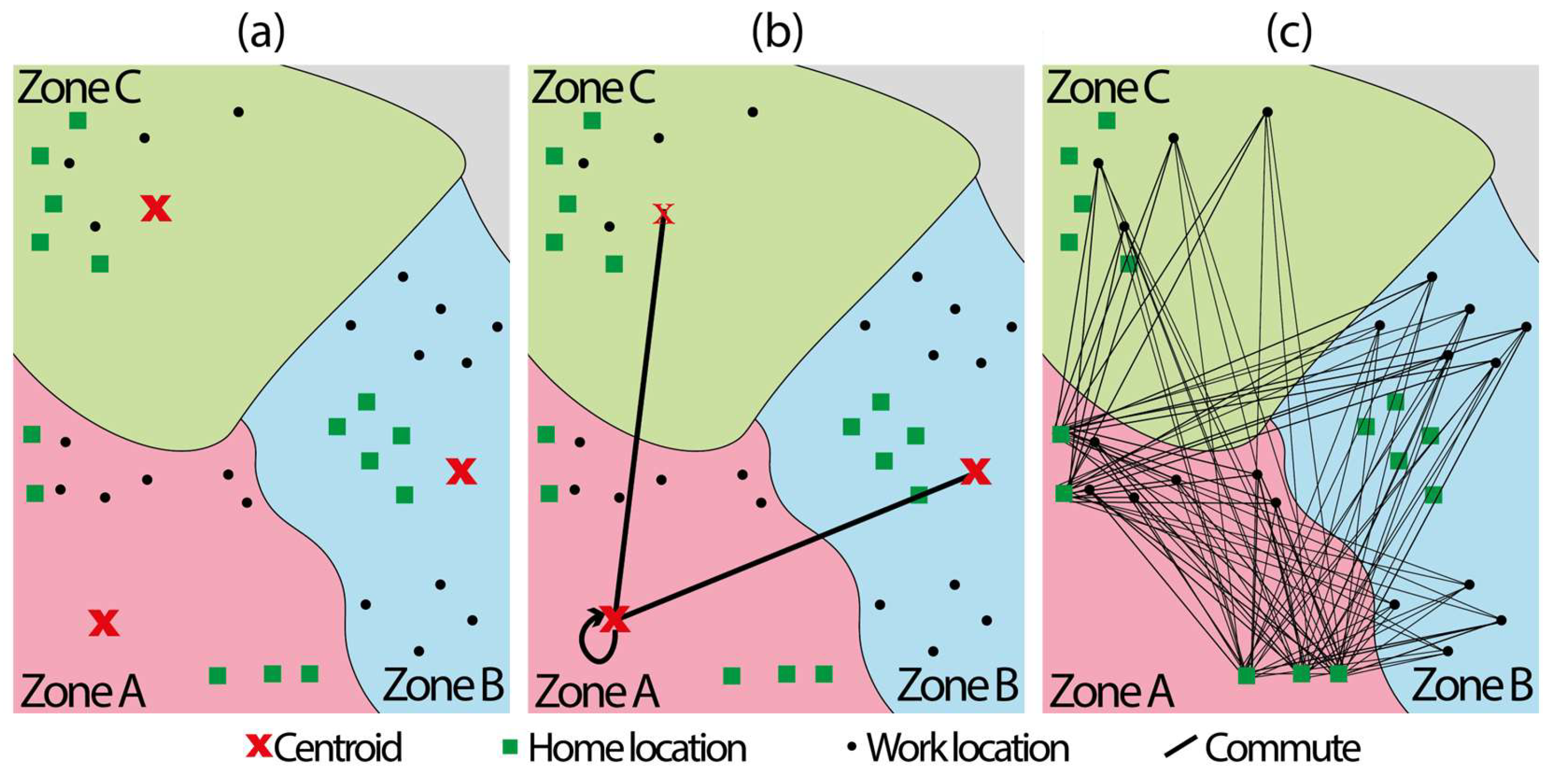
Studies on accessibility commonly calculate the travel time between the centroids of zones (e.g., census tracts and traffic zones), as in, for example, [17,19,23,24,30]. While centroids might be a valuable approximation, their location can substantially influence travel time, particularly within public transport systems. A centroid placed within a transport hub may result in an underestimation of the travel times required to most Points of Interest (POI) within a neighbourhood. A centroid less conveniently located may require a walk or a bus ride to reach the destination, thereby overestimating the travel duration to most POIs in the neighbourhood. Using centroids also raises the question of whether to locate these where most people live, instead of the geographical centre. To avoid any of this, the study uses the travel duration between the exact coordinates of both home and work locations. Hu et al. [28] raised similar concerns, stating that the zones commonly used in accessibility studies were predominantly designed for census purposes, which may not represent the actual distribution of employment opportunities correctly. They also bemoan that the job accessibility levels are likely to change just by reshaping zone boundaries and dimensions. They also criticise the use of centroids, as these assume that all workers would work and live in a zone’s core—leading to significant errors in larger zones [28]. They applied an ‘areal interpolation method’, named dasymetric mapping, to redistribute their count data (i.e., aggregated by traffic zones) to a much finer 500 m grid using auxiliary data, such as population density [28]. While the present study uses a much finer grid (i.e., 30 m), the underlying principle stays the same. In earlier work, various authors have voiced their concerns about aggregation errors and the impact of altering the special unit of reference on the results (e.g., [40,41]). Further details on how the accessibility calculation has been modified and the rationale for it have been provided in Section 3.1 and Section 3.5.

3. Materials and Methods

3.1. Workplaces and Home Locations

This study uses a commuter flow dataset, like various other scholars (e.g., [19,23,24]). To determine the number of employment opportunities within each MSOA (i.e., Middle Layer Super Output Area), this study aggregates the 2011 commuting dataset [42]. The dataset splits England and Wales into more than 7000 MSOAs. Each MSOA has between 2000 and 6000 households [43]. Since this study assumes that individuals commute to their office on working days, those working from home or overseas, etc., were removed from this dataset. The number of workplaces within each MSOA was divided by 100 to reduce processing power required for routing. This denominator ensured that sufficient workplaces remain even in predominantly residential or rural MSOAs. The distribution of the population within each MSOA was determined based on the High-Resolution Population Density Maps [44], which have an arc-second block resolution. This corresponds roughly to a 30 m grid [45,46]. The population density was inferred using computer vision algorithms to identify buildings on satellite imagery in conjunction with the best available census datasets [45]. In short, this paper aggregates the commuting dataset to determine the number of job opportunities within each MSOA. The geographic distribution of jobs in this study, therefore, aligns with the 2011 spatial arrangement (i.e., a time when working from home was less prevalent). The high-resolution map served primarily to link coordinates to built-up areas within each MSOA. The exact location of each workplace was generated by randomly choosing a grid coordinate located within the MSOA. Sampling with replacement was applied, and the probability of each grid coordinate was weighted by the population distribution [44]. The population density data were mapped to each MSOA using a shapefile [47]. The rationale for this approach is explained in Section 2.5 and Section 3.5.

Five home locations were randomly selected within each MSOA, assigning higher probabilities to more densely populated arc second blocks. It was not necessary to use a figure that closely resembles the actual number of people residing within each MSOA, as this study quantifies the reachable employment opportunities. Five locations were deemed sufficient to create a representative sample of start locations of each MSOA. The sensitivity analysis in this paper confirms that this approximation has only limited effect on the results.

The process was inspired by the creation of work and home locations illustrated in Schnieder [48] (focused on parcel deliveries) as well as Schnieder [3] and Kelly et al. [49] (remote working hubs/co-working spaces) [48]. Python 3.13 and a vast selection of libraries has been utilised, including Pandas [50], GeoPandas [51], matplotlib-map-utils [52], Matplotlib [53], matplotlib_scalebar [54], Seaborn [55], NumPy [56], Shapely [52,54,57], and SciPy [58].

3.2. Scenarios

The effective accessibility scores for a bicycle, e-bike, s-pedelec and two cars (i.e., at different affordable price points) are compared in this study (

Table 1. Definitions.

Vehicle	Definition
Bike	A conventional bicycle only propelled by pedals and only powered by a human.
e-bike	An Electrically Assisted Pedal Cycle (EAPC) that is commonly referred to as an ‘e-bike’ or ‘e-cycle’ in the UK markets [59] or as a pedelec in, for example, Germany [60]. Equipped with pedals [59]. Electric motor up to 250 W [59]. Electrical assistance up to 15.5 mph [59]. No insurance, registration, or tax required [59].
s-pedelec	A bicycle with pedal support of up to 45 km/h.
Car	A car cost that is equivalent to the average motoring outlay in the UK.
Car 2	A car priced at a level comparable to the motoring budget by those in the lowest income decile.

). The concept and legal definition of an e-bike are subject to a level of divergence across national contexts and regulatory frameworks. With the study taking place in the United Kingdom, the terminology which prevails in the context of the UK has been adopted. The only exception to this is the lesser-known term s-pedelec (in the UK).

3.3. Travel Distance and Duration

The daily commute from each home location to every workplace has been computed. The roundtrip travel duration and distance were determined using an Open Source Routing Machine (OSRM) [61] instance (hosted locally). The street network was provided by OpenStreetMap (OSM) [62]. The OSRM bike profile has been used for all types of bicycles and the car profile for both types of cars [63]. In line with the findings of a naturalistic cycling study in Germany (17,000 km recorded), the average speed of an e-bike was increased by 2 km/h and for an s-pedelec by 9 km/h [60]. The time required to park a car was not included, as finding a secure parking spot for an expensive s-pedelec might also present a challenge in certain areas.

3.4. Cost of the Commute

It is inherently troublesome to define representative values for the cost of commuting by car or bicycle. Individual expenditure markedly differs, reflecting the role of social or prestige motivations, gathered alongside economic constraints. Selecting the most cost-effective car or bicycle will not be representative of the actual amount paid, while the average expenditure greatly overestimates the true costs that less affluent individuals can afford. The economic burden may also be influenced by certain tax incentives or other financial mechanisms available to eligible employees (e.g., commuter allowance and company cars). To navigate this inherent difficulty, the applied costs were informed by various sources to ensure alignment with the prevailing consensus and statistics compiled by the relevant literature. International currencies were converted using the current exchange rate. An amount of £35 per month (i.e., around 40 €), split across 21 working days per month, was assumed to be the total operating cost of commuting by bicycle. This financial expenditure exceeds those commonly reported in scholarly discourse (e.g., 475 € per year [17] or 1 € per day [64]). This was implemented to avoid the perception of only favouring this mode of transport.

The median retail value of an e-bike, purchased under the Cycle to Work scheme, was £750 [65]. Those paying the basic tax rate had a median spend of £650, compared with £1000 by higher rate taxpayers [65]. Due to the low energy consumption, the cost to charge an e-bike is negligible in light of other expenses [66]. Synthesising these values, the study assumes a fixed monthly cost of £48 per month for e-bikes. As this monthly cost enables a post-warranty replacement, the consideration of maintenance was deemed unnecessary. With the expected and reported operational life of e-bikes and their batteries generally exceeding 2 years, this value should represent, or slightly overestimate, the costs that can reasonably be expected to operate a socially appropriate e-bike. It is certainly the case, given that employees can potentially save 32% to 47% on the loan of an e-bike using the previously referenced Cycle to Work scheme [65]. Appraising the cost of an s-pedelec is markedly more intricate since the higher acquisition costs render the Cycle to Work scheme more lucrative [65]. The financial remittance offered by these schemes depends on the individual’s personal income. To circumvent any bias, two cost levels were compared (i.e., £96 and £192 per month).

The cost of car ownership was taken from Schnieder [4]. The fuel costs are assumed to be £0.075/km, informed by the current average UK retail (‘pump’) prices [67] and the average fuel consumption [68]. The cost to operate a car was set as £269.80 per calendar month plus £0.16 per km, guided by [69,70,71]. As this value might not be representative of the most reasonably priced car, affordable to the less affluent, the outlay was simply halved to represent this option. Thereby, the costs assumed closely resemble the UK household motoring expenditure for those owning a car and belonging to the lowest decile income group [69]. With the average expenditure amongst the highest-income group being £155.90 per week [69], this cost halving represents a significant underestimation of motoring expenditure by the average UK household.

Table 2. Costs.

Vehicle	Costs Per Month	Cost Per km
Bike	£35 per month
e-bike	£48 per month
s-pedelec	£96 per month
Expensive s-pedelec	£192 per month
Car	£269.80 per month	£0.16 per km
Car 2 (reasonably priced)	£134.90 per month	£0.08 per km

lists the operating costs assumed in this study. Since income is usually earned on working days, the monthly costs are split only across an assumed 21 working days per month. While these costs may not be representative of the expenditure in Europe, they correspond to the following EUR-equivalent values, converted using the average exchange rate over the last year according to the European Central Bank [72]: Bike €40.29, e-bike €55.25, s-pedelec €110.50, expensive s-pedelec €221.00, Car €310.55 per month and €0.21 per km, Car 2 (reasonably priced) €155.27 per month and €0.11 per km.

3.5. Calculation of the Effective Accessibility Score

A more detailed explanation of the calculation of the effective accessibility score can be found in Schnieder [18]. In short, the score measures the ease of reaching nearby employment opportunities using a specific mode of transport [19,23]. While cumulative opportunity measures, as used in this study, are often praised for being readily comprehensible, treating all destinations within a time or distance threshold as equal may inadequately represent perceived opportunities [24]. A gravity-based measure can mitigate this limitation by discounting the value of destinations based on their distance [24]. Owing to the strong correlation between both measures [19,23], the cumulative accessibility was implemented in this study.

The cumulative opportunity measure version of this score is calculated in line with the academic consensus using the Equation (1) (i.e., the Hansen equation) and Equation (2) as published in Mann et al. [73]:

$$A_i=\sum _j{O}_{j}f\left(C_{ij}\right)$$

(1)

$$f\left(C_{ij}\right)=1 if C_{ij}\le t, else f\left(C_{ij}\right)=0$$

(2)

where

$A_i$—Accessibility for location i;

$O_j$—Number of jobs or other opportunities at destination j;

$C_{ij}$—Travel costs (i to j);

$f\left(C_{ij}\right)$ —Impedance function.

While the above equations were used exactly as they are in this study, there are two distinct deviations from the usual academic approach, in which the novelty contribution of this paper lies:

First, $C_{ij}$ is in many academic studies equal to the time spent travelling. This study, however, applies the effective speed concept and uses the combination of travel duration and work hours needed to offset those expenses. The overwhelming advantages of accounting for both time components are highlighted in [9,15,16,17,74]. Five hourly wages were used (i.e., £10, £12.21, £15, £20, and £30) to convert the transport costs into the work duration required to earn these. While a value below the minimum wage may appear counterintuitive, it can represent an opportunity cost, or a value of time [4]. Second, as explained in Section 2.5 [17,19,23,24,30], this study uses exact coordinates of both home and work locations, as shown in Figure 1, to calculate the time spent commuting. After this, the accessibility values $A_i$ of the five home locations within each MSOA are aggregated. Since there is only one workplace at each workplace $O_j$ is always equal to one in this study.

To capture individuals’ experiences lived more closely, a logarithmic scale was applied, and the raw score was normalised between 0 and 100, as illustrated in Equation (3). As a result, increasing the number of employment opportunities one can reach from an under-served location—even by a few—may be apposite. However, the same increase might be considered irrelevant in neighbourhoods where jobs are plentiful. The logarithmic transformation was applied to the raw score plus 1 to ensure that 0 reachable jobs will not raise an error as suggested in [75]. The minimum–maximum normalisation provides a linear transformation while keeping the relationship among the original data [76]. Despite the [0, 1] interval being commonly used in academic research, a [0, 100] interval was chosen, as it appears more intuitive. The equation was first published in Schnieder [18].

$$X_i={\displaystyle \frac{\mathrm{l}\mathrm{o}\mathrm{g}(x_i+1)-\log (x_{min}+1)}{\log (x_{max}+1)-\log (x_{min}+1)}}\ast 100$$

(3)

where

$X_i$—Final effective accessibility score for MSOA i;

$x_i$—Raw effective accessibility score for MSOA i (i.e., the $A_i$ values of all five home locations per MSOA combined);

$x_{min}$—Smallest raw effective accessibility score;

$x_{max}$—Largest raw effective accessibility score.

While there are distinct differences, some may notice that the logarithmic scale and the normalisation were partly adopted from the Walk Score (see [39] for reference).

3.6. The Study’s Limitations

The 2011 commuting data were chosen, as the following census, 10 years later, was impacted by the COVID-19 pandemic. Also, several recently published papers still use the same data as this study: Tengilimoglu et al. [77] evaluated the suitability of the current infrastructure for autonomous vehicles, and Shen [77,78] proposed the ‘Relative Accessibility Gain’ measure. To estimate the time-saving benefits and mode shifts encouraged by improvements in sustainable modes of transport, Ma et al. [79] used the 2011 data as a baseline. The paper submitted by Liu et al. [80] in December 2025 still relied on this dataset.

The rise of hybrid working arrangements holds relatively minimal pertinence in this study, since the focus is on a comparative evaluation of (electric) bicycles and cars. The increased prevalence of working from home leads to a reduction in both (i) the availability of office-based jobs and employment opportunities and (ii) the number of individuals for whom this study is relevant (i.e., only those working 5 days a week in the office). Note: Hybrid working or working from home accounted for 38% in April 2025 in the UK [81]. It is entirely plausible that the current geographic distribution of workplaces has changed and may no longer fully represent a scenario in which employees commute to the office 5 days per week. As the simulation is designed to reflect the latter scenario, 2011 may be more appropriate (i.e., 10.3% home or hybrid working arrangements [82]). Nevertheless, other datasets used in this study are more recent (e.g., the population density data). The routing was also performed on the latest OSM street network data.

Furthermore, any subjective times (i.e., searching for a parking spot) that would negatively affect commuting by car more than by bicycle were not considered. This ensures that bicycles are not unduly favoured in this analysis.

Analogous to many studies, all occupied jobs are considered (i.e., attraction-accessibility measure) [83]. In practice, the educational background, personal preferences, and job market shape the prospect of employment opportunities for an individual [84]. This is not a significant limitation, as this study analyses the accessibility levels offered by bicycles, e-bikes, s-pedelecs, and cars—rather than examining social inequalities.

In short, the objective of this paper is to compare e-bikes with cars for those who always commute to the office (i.e., no hybrid working). The objective is not to illustrate the current commuting conditions, social inequalities, or the labour market.

4. Results

4.1. Job Accessibility (Travel-Time Based)

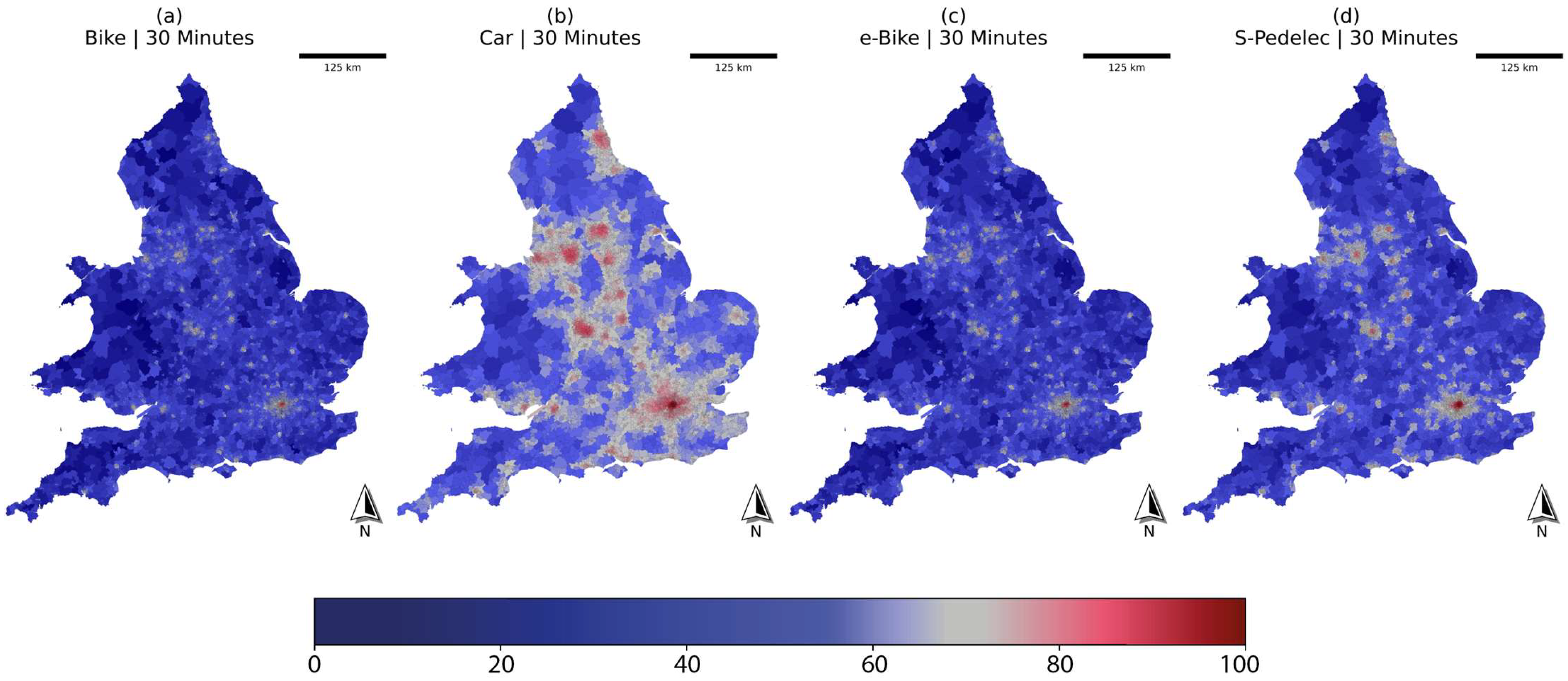
Figure 2 visualises the ‘job accessibility’ score (travel-time based) for a 30 min roundtrip. It therefore visualises the jobs reachable within the 15 min context. The inherent expedience of commuting in private cars is obvious when only the time behind the wheel is accounted for. The distinctions between bicycles and e-bikes are rather subtle, while s-pedelecs provide a discernible gain.

Metropolitan areas stand out due to their high levels of accessibility, while the limited opportunities in peripheral regions may indicate spatial inequalities. However, those residing in densely populated areas may face increased competition for jobs compared with those in less crowded areas. For the reader unfamiliar with the UK, the size of each MSOA (i.e., geographical unit) corresponds with the population density, to a certain degree, given that each includes between 2000 and 6000 households [43].

4.2. Effective Accessibility Score

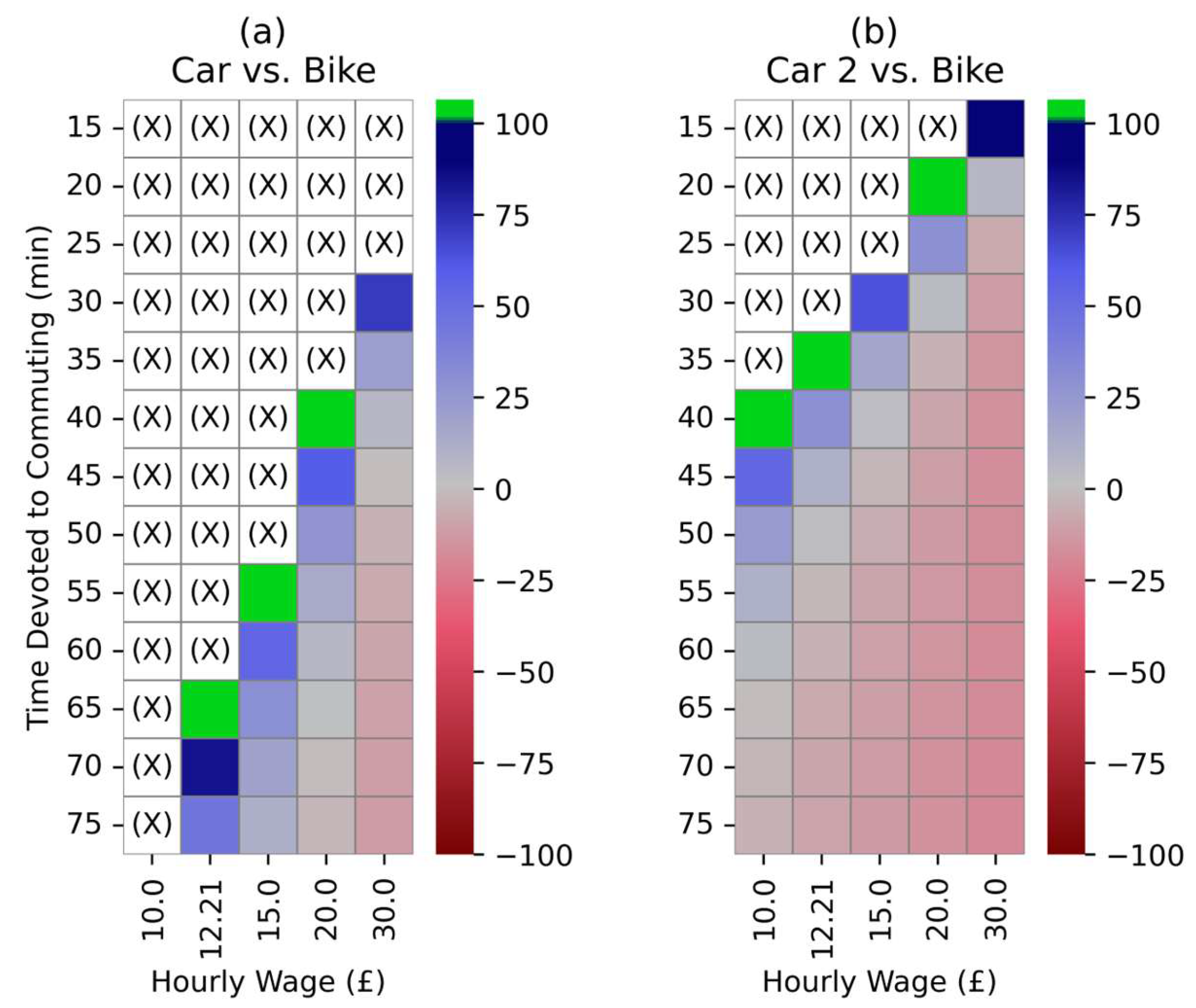
Figure 3a depicts a comparison of the effective accessibility scores of bicycles with those of cars for different hourly wages and time thresholds. The score also considers the time at work to finance the commute. The figure visualises relative percentage changes, with cells in red representing the superiority of cars and blue denoting the bicycles’ leading position. An (X) indicates the unattainability of employment opportunities by cars, as the duration necessary to accrue the required funds outstrips the available time. A green cell in the figure signals an increase above 100%. Commuting by bicycle can exceed the score of cars by multiple folds if only a few minutes are available to drive. This is especially pertinent for lower time and income thresholds. However, these income and time combinations are somewhat sensitive towards the assumptions made, as shown in the sensitivity analysis, and therefore the exact increase should be considered with a degree of caution. Individuals with an hourly rate of £10 or below are unable to reach any job by car within 75 min due to an inability to acquire the funds in that specific timeframe. With individuals at an hourly rate of £20 or £30, the effective accessibility scores become comparable (less than a 5% difference) for time thresholds of 65 min and 45 min, respectively.

When opting to buy a reasonably priced car, commuting becomes notably more competitive, even for those on a low income, if they are willing to spend enough time commuting or working (Figure 3b). In this comparison, thresholds of 25 to 65 min enable cars to stay competitive depending on the driver’s income. Note: The expenses associated with car commuting in this comparison are underrepresentative of the broader population in England and Wales. It is only characteristic of the lowest income decile, which own a car.

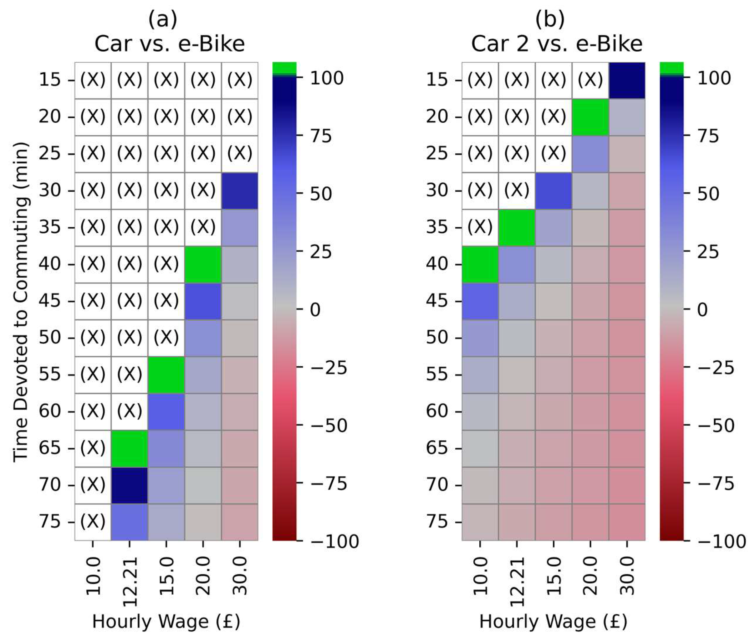
Figure 4 contrasts the effective accessibility scores for an e-bike with those for a car. Although the outcomes resemble Figure 3 (bike vs. car), the point at which cars reach competitive levels occurs at a slightly higher threshold (up to 5 min).

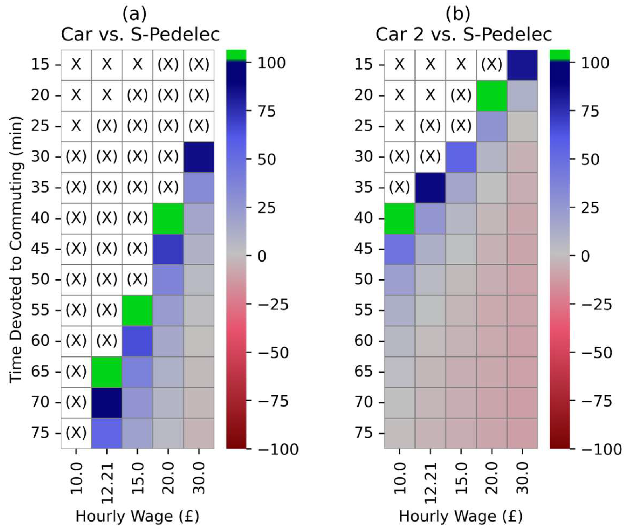
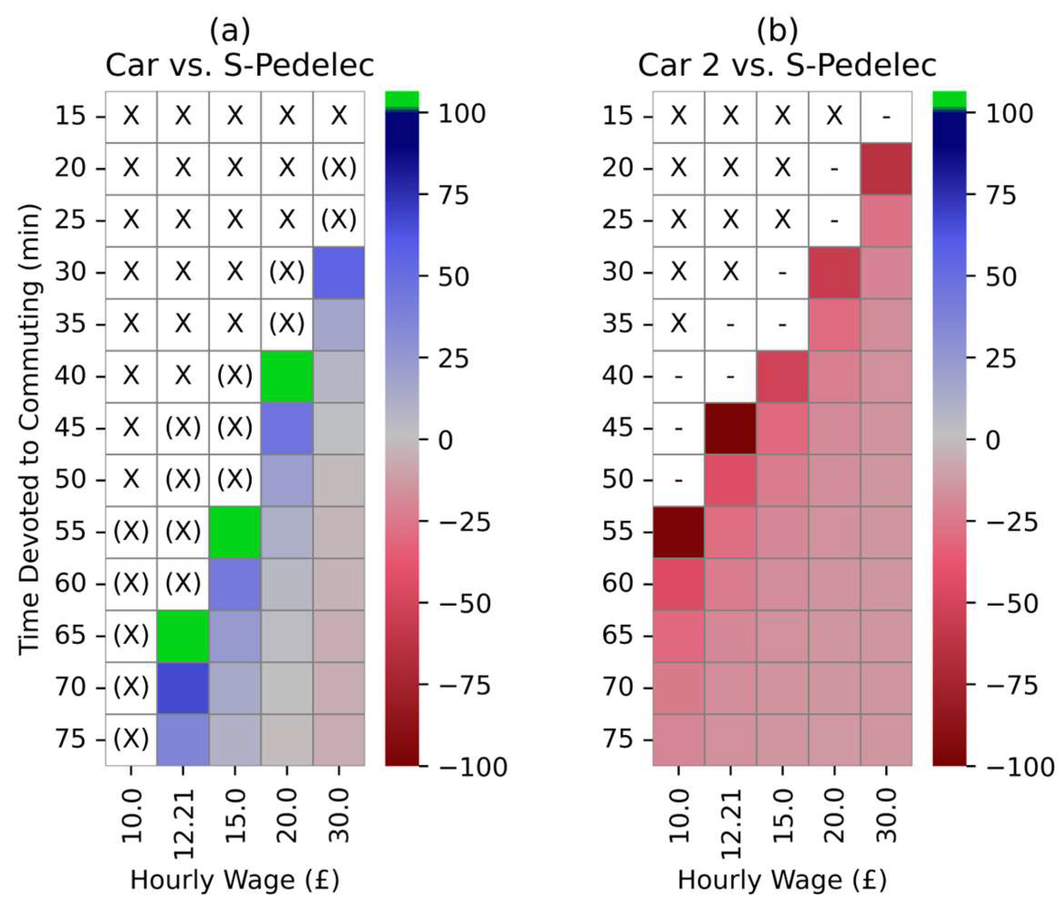
This trend is even more pronounced in Figure 5, which juxtaposes s-pedelecs with cars. Cars only ever achieve competitiveness when the threshold reaches 60 min for those with a £30 hourly wage. For all remaining combinations of time thresholds and income levels considered in this study, s-pedelecs attain higher effective accessibility scores.

Even if cyclists opt to purchase a rather expensive s-pedelec (£192 per month), cars only attain competitiveness for individuals earning £20 ph with over an hour at their disposal or for those earning £30 ph with at least 45 min available (Figure 6). The reason lies in the limited speed advantage of cars relative to s-pedelecs, especially in urban environments. Expensive s-pedelecs are unable to match the effective accessibility levels offered by reasonably priced private vehicles.

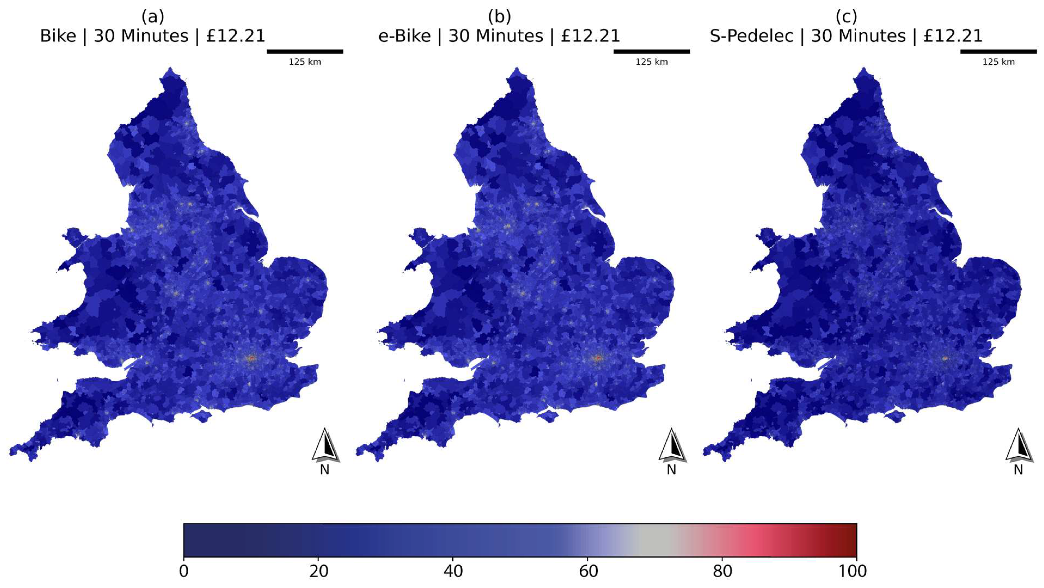
Figure 7, Figure 8 and Figure 9 highlight the geographic differences in the effective accessibility scores. For those with an exceptionally constrained time budget (i.e., 30 min), s-pedelecs may not offer an advantage over bicycles or e-bikes. In Figure 7, London once more emerges in the geographic comparison as a major hub for employment opportunities. Notwithstanding that, the competitive pressure for jobs may be more pronounced here.

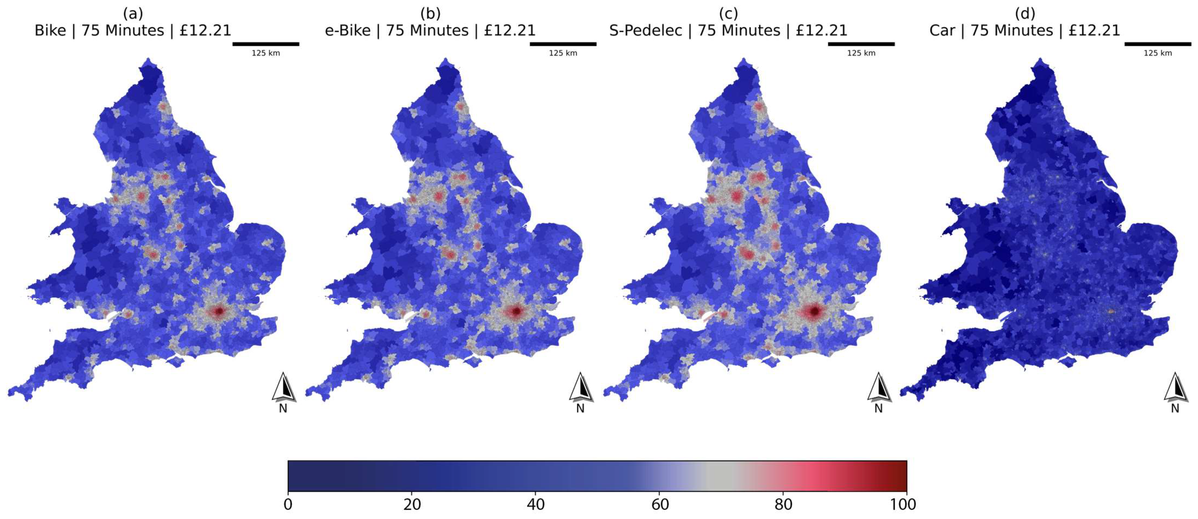
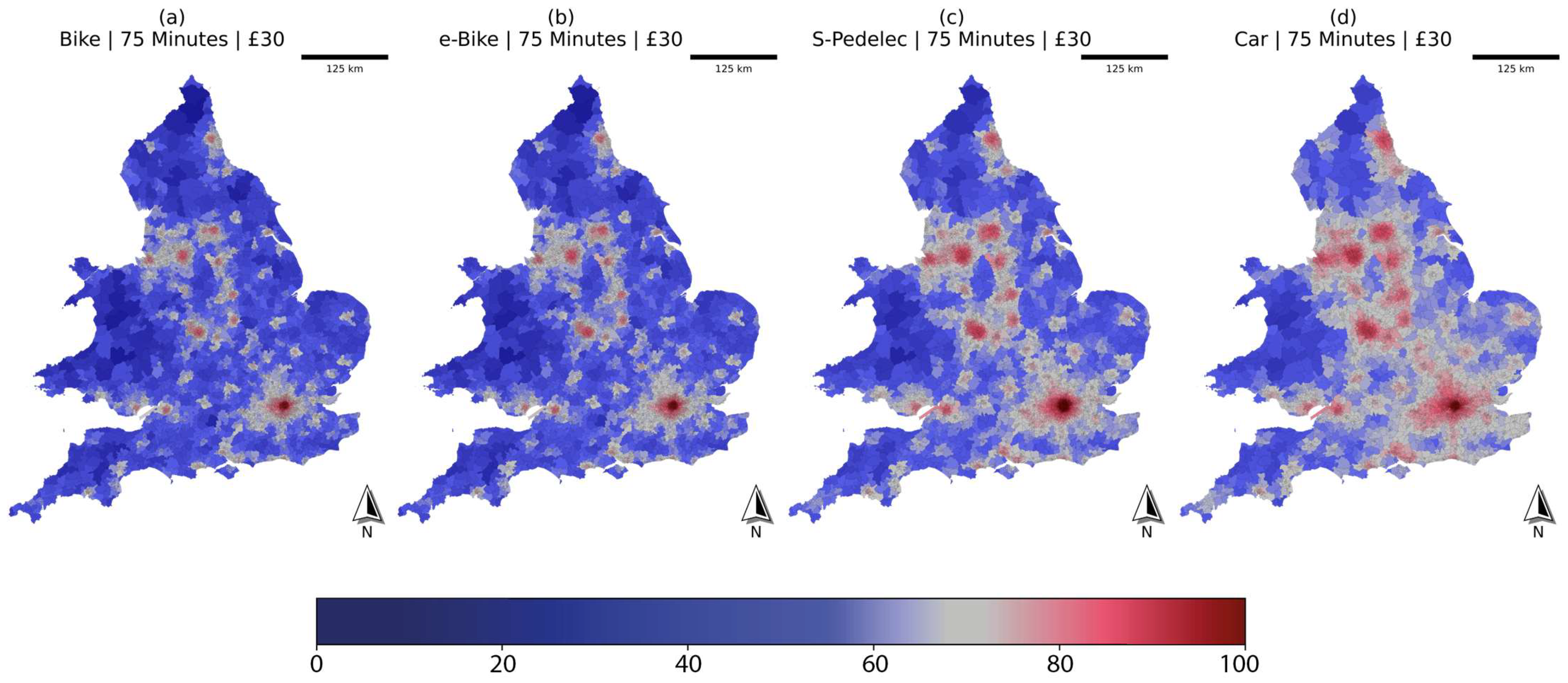
With the time budget prolonged to 75 min (Figure 8), nearly all major urban agglomerations attain high effective accessibility scores—if active modes of transport are utilised instead of cars.

Raising the hourly wage to £30 results in universally high effective accessibility scores in urban areas (Figure 9). For a more detailed geographic comparison, the reader is referred to the box plots after these maps.

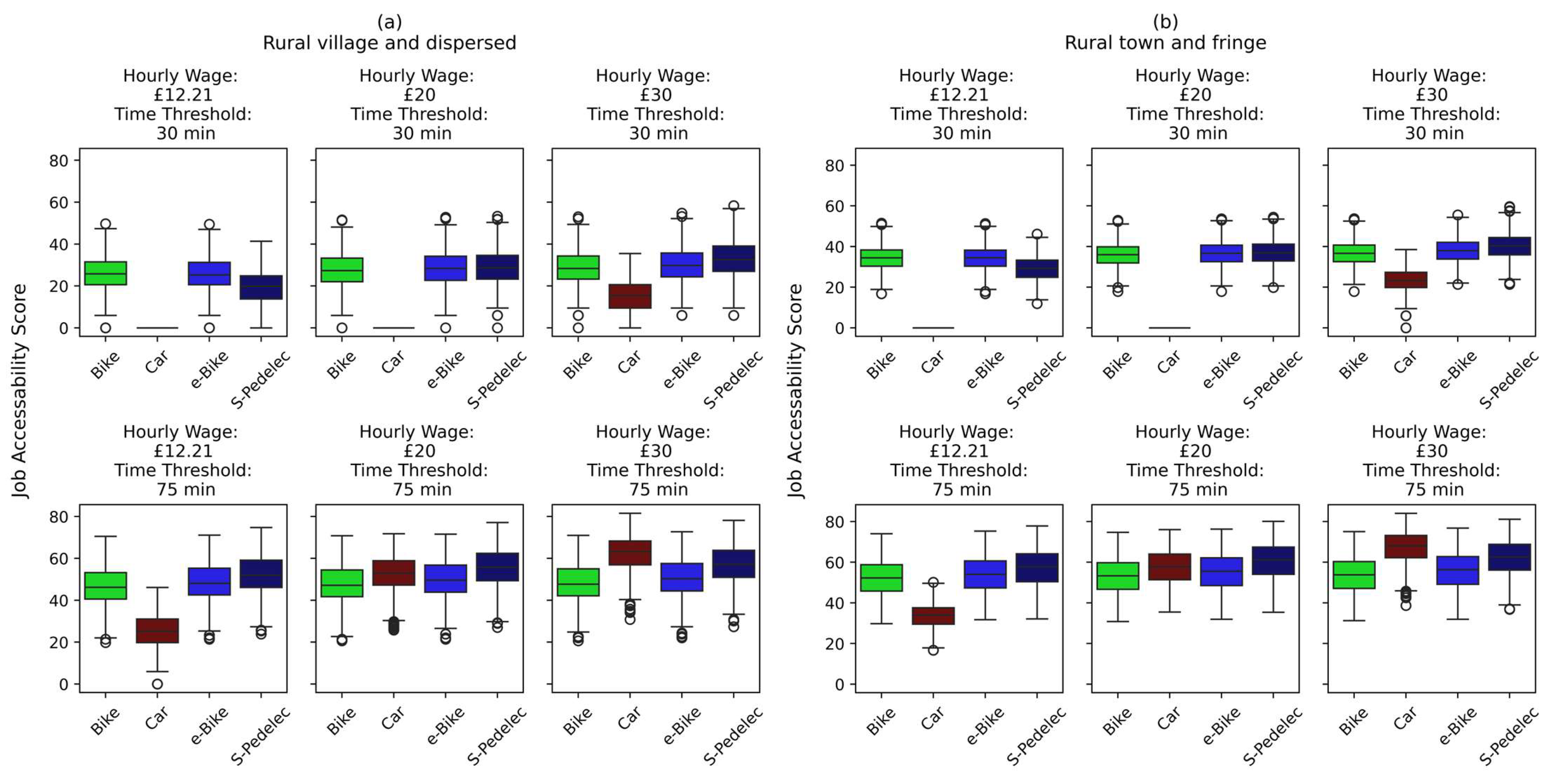
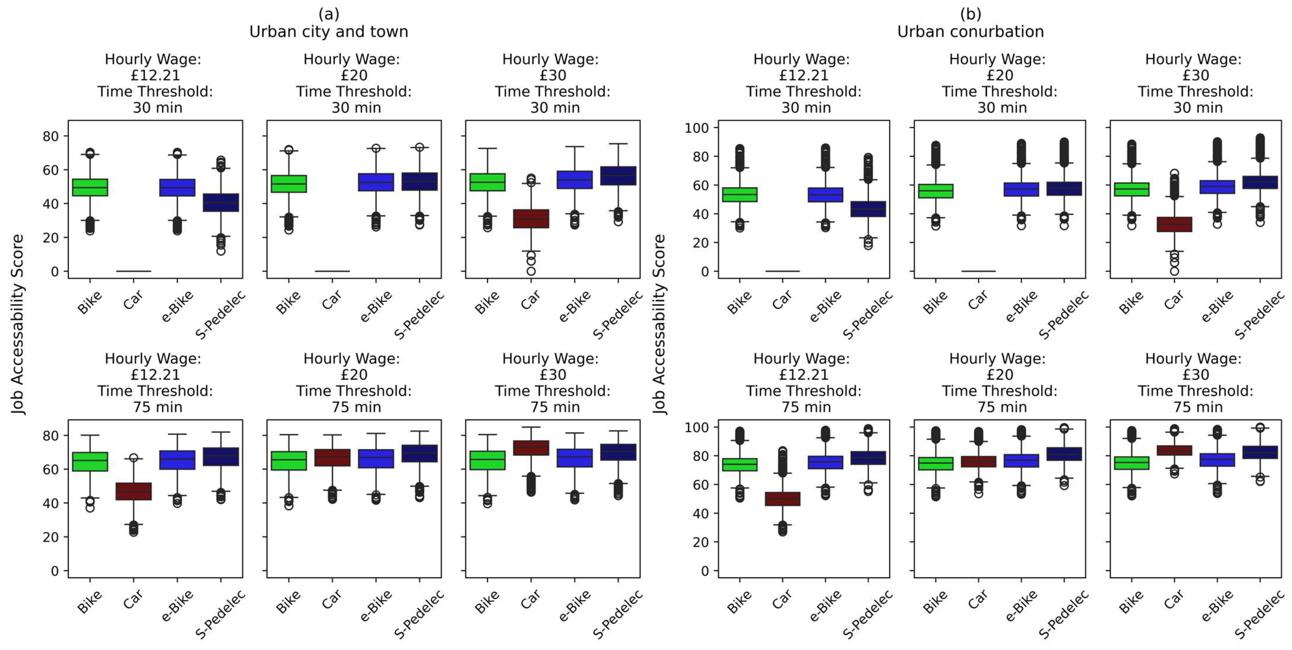
Figure 10 and Figure 11 visualise the effective accessibility scores for four different area types ranging from rural to urban. The dataset [85] provided by the ONS was utilised for the classifications of the MSOA. To reduce the number of figures, two area types were grouped together. The figures highlight the stability of the results across different area classifications. Those with the highest income and available time may wish to drive a car. Conventional bicycles and e-bikes are most suitable for those earning minimum wage and with limited available time. S-pedelecs are the most suitable option for all other groups of people.

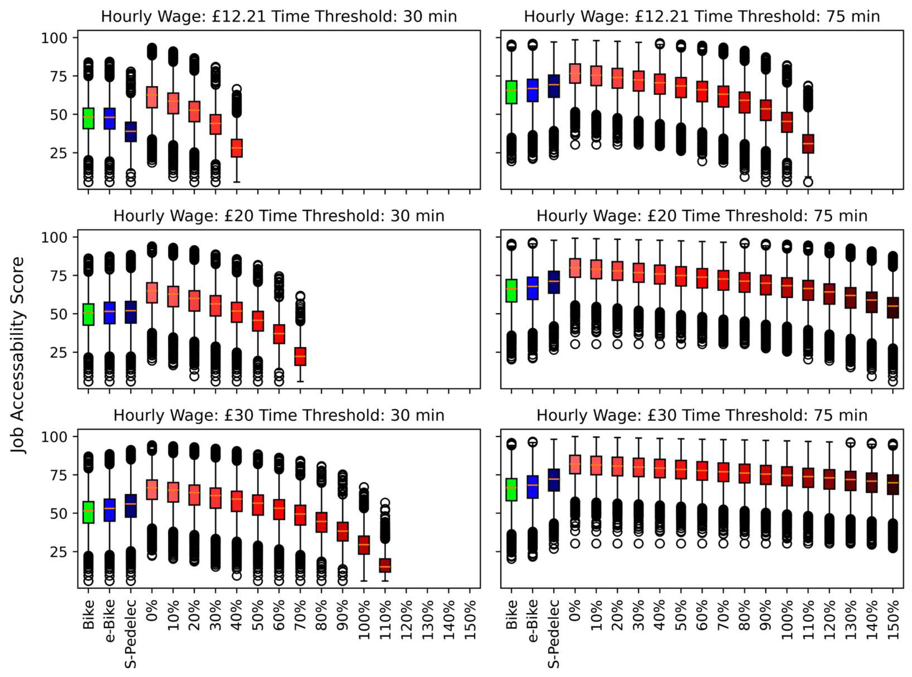
Across all previous analyses reported in this paper, the entirety of cars’ fixed costs have been taken into account. In reality, a more nuanced consideration may be warranted: (i) individuals borrowing a vehicle from a friend may only cover the variable costs (e.g., fuel, wear and tear); (ii) an accounting of 5/7 of the fixed costs may be appropriate when the vehicle is used by the owner’s partner/relatives on weekends; (iii) excessive parking fees in certain areas may render the ‘statistical average outlay on motoring needs in the UK’ a gross underrepresentation. To account for the variation in fixed costs, Figure 12 illustrates the effective accessibility scores for a varying share of fixed costs being considered. This figure underscores the critical role of removing any car ownership requirements. If car ownership is a prerequisite (i.e., no (or a fraction of) the fixed costs are accounted for), commuting by car becomes the most expedient choice for many individuals.

4.3. Sensitivity Analysis

A sensitivity analysis was conducted to evaluate the influence of the exact locations (i.e., homes and workplaces) as well as cost and speed assumptions on the output of the digital model.

The exact coordinates of individuals’ homes, as well as employment opportunities, have a degree of randomness, as explained in the methods. The simulation was repeated twice (in addition to the reference run) to evaluate the extent to which the results are influenced by random variations rather than by a consistent underlying pattern.

The variability across the simulation runs is generally minimal across all combinations of income and hourly wage. For cars (

Table 3. Analysis of the digital model’s sensitivity (cars).

Hourly Rate	Available Time	Comparison	R2	Pearson	NRMSE
£12.21	75 min	1 vs. 2	0.9086	r = 0.955, p < 0.001	0.0389
		1 vs. 3	0.9087	r = 0.954, p < 0.001	0.0389
£20	45 min	1 vs. 2	0.8380	r = 0.920, p < 0.001	0.0544
		1 vs. 3	0.8324	r = 0.916, p < 0.001	0.0554
£20	75 min	1 vs. 2	0.9803	r = 0.990, p < 0.001	0.0202
		1 vs. 3	0.9807	r = 0.990, p < 0.001	0.0200
£30	30 min	1 vs. 2	0.7526	r = 0.876, p < 0.001	0.0714
		1 vs. 3	0.7467	r = 0.872, p < 0.001	0.0722
£30	45 min	1 vs. 2	0.9493	r = 0.975, p < 0.001	0.0277
		1 vs. 3	0.9531	r = 0.977, p < 0.001	0.0266
£30	75 min	1 vs. 2	0.9894	r = 0.995, p < 0.001	0.0147
		1 vs. 3	0.9899	r = 0.995, p < 0.001	0.0144

), the alignment is lowest for an hourly wage of £20 and 45 min, as well as for £30 and 30 min. Due to the high cost of car ownership, only a limited time is available to drive in these instances. Hence, the precise location of a home or a place of work does matter for those cases. However, once the time threshold is increased, the high R² values and Pearson correlations, combined with a low NRMSE, highlight the model’s robustness.

A similar pattern can be observed in the sensitivity analysis of the commuting by bicycle simulation (

Table 4. Analysis of the digital model’s sensitivity (bicycle).

Hourly Rate	Available Time	Comparison	R2	Pearson	NRMSE
£12.21	30 min	1 vs. 2	0.9273	r = 0.963, p < 0.001	0.0366
		1 vs. 3	0.9205	r = 0.960, p < 0.001	0.0383
	45 min	1 vs. 2	0.9541	r = 0.977, p < 0.001	0.0296
		1 vs. 3	0.9556	r = 0.978, p < 0.001	0.0291
	75 min	1 vs. 2	0.9770	r = 0.988, p < 0.001	0.0228
		1 vs. 3	0.9768	r = 0.988, p < 0.001	0.0229
£20	30 min	1 vs. 2	0.9368	r = 0.968, p < 0.001	0.0338
		1 vs. 3	0.9310	r = 0.965, p < 0.001	0.0353
	45 min	1 vs. 2	0.9576	r = 0.979, p < 0.001	0.0293
		1 vs. 3	0.9591	r = 0.979, p < 0.001	0.0288
	75 min	1 vs. 2	0.9785	r = 0.989, p < 0.001	0.0222
		1 vs. 3	0.9780	r = 0.989, p < 0.001	0.0225
£30	30 min	1 vs. 2	0.9391	r = 0.969, p < 0.001	0.0329
		1 vs. 3	0.9354	r = 0.967, p < 0.001	0.0339
	45 min	1 vs. 2	0.9593	r = 0.980, p < 0.001	0.0286
		1 vs. 3	0.9603	r = 0.980, p < 0.001	0.0283
	75 min	1 vs. 2	0.9792	r = 0.990, p < 0.001	0.0218
		1 vs. 3	0.9787	r = 0.989, p < 0.001	0.0221

).

A second sensitivity analysis was conducted to evaluate the effect of changing the costs or travel duration. The effective accessibility scores remain relatively insensitive to a 20% increase or reduction in the travel duration, with changes of less than ±3 score points across all vehicles.

Altering the cost by 20% tends to produce only marginal variations. For bicycles and e-bikes, the score is changed by less than ± 1.5 effective accessibility score points. The score of s-pedelecs in most cases changed by less than ±2.3 score points, apart from the situation where the hourly wage is £12.21 and the time threshold is 30 min. Like before, this exception of a high sensitivity appears in instances with limited travel time due to the increased costs. The same applies to both car variants, where the score is usually changed by less than ±5 score points. However, for combinations where car commuters can only reach a few jobs, the score changes by just over ±10 score points.

Previously, no employment opportunities could be reached with a reasonably priced car, a time budget of 30 min, and an hourly wage of £12.21. Through an additional 20% reduction in expenses, some employment opportunities could be attained.

Both sensitivity analyses highlight that the combination of income with limited available time to travel is rather sensitive to the randomness in the placement of locations, as well as the cost and speed values chosen. This indicates that these instances should be seen with caution. A detailed figure highlighting this can be found in Schnieder [18].

5. Discussion

This research paper undertook a comparative analysis of the ‘access to employment opportunities’ in England and Wales, offered by bicycles, e-bikes, s-pedelecs and cars, using the concept of the effective speed. The latter extends the calculation of the average speed beyond the commute itself by considering the working hours necessary to earn the income required to finance the journey. S-pedelecs and, to a lesser extent, e-bikes and conventional bicycles offer, in various settings, the highest effective accessibility scores. Cars should only be considered by those with sufficient hourly income and a willingness to devote sufficient time towards commuting or earning the money to fund it. The results of this study highlight significant regional differences in the effective accessibility scores. However, the results require careful consideration, considering the increased competition for jobs in densely populated urban agglomerations.

The conclusions drawn from these evaluations stand in stark contrast to those commonly drawn by accessibility studies, apart from Vale [17] and Schnieder [18]. Evidence from previous studies on job accessibility often suggests a sombre trajectory. For example, Mocanu et al. [5] proclaimed that commuting by public transport is not a competitive alternative for all regions in Germany, given that travel durations last almost three times longer. Similar conclusions were drawn by Kosmidis et al. [6] in Nord-Jæren (Norway), Pritchard et al. [7] in São Paulo (Brazil) and Zini et al. [8] in Rome and Turin (Italy) [6].

Beyond the context of accessibility studies, the research on the effective speed concept has extensively documented that the time efficacy of travelling by car is often overvalued [9]. The temporal burden of spending time at work to offset commuting expenses is somewhat invisible and commonly eludes the drivers’ full awareness [10]. When accounting for the time at work, the car’s speed advantage is significantly diminished [11]. Consequently, this research seeks to advocate the integration of the effective speed concept into accessibility evaluations, reflecting the approach proposed by Vale [17].

6. Policy Recommendations

With the need to reduce emissions and fuel consumption, many technologies and policies have been proposed to achieve this goal. However, these strategies often increase costs (e.g., new technologies), are more time-consuming (e.g., different modes of transport), or prompt consumers to forgo or change travel plans (e.g., not flying on holiday or to business meetings) [9]. The implementation of such strategies may pose a challenge in cost, quality- and time-driven societies [9]. However, this paper provides a solution to this problem by highlighting the potential that commuting by bicycle may not be as slow as it seems. By simply combining the costs (i.e., the duration to earn the funds) and the time spent commuting into the equation, more affordable modes of transport like bicycles become faster—from an effective speed perspective. Hence, the first policy recommendation from this paper is to spread the word of the effective speed concept and use this concept to guide policy decisions (policy recommendation 1). Some academics go even further by advocating the ‘social effective speed’ which also considers the external costs of a mode of transport [74].

Admittedly, the realisation of any recommendations encouraged by this study hinges on the removal of barriers restricting bicycle usage. A fully integrated and well-structed bicycle network and secure parking constitute a pre-requisite to successful implementation [86] (policy recommendation 2). Additional impediments, including physical exertion, sharing roads with a motor vehicle [87], health conditions that prevent cycling [88], steep hills [88], long trip distances and weather conditions [89], necessitate targeted interventions to address these obstacles. Any pre-requisite for car ownership must be addressed (policy recommendation 3), as the associated fixed expenses, such as the initial purchase, become inherently unavoidable. In such circumstances, individuals might only account for fuel costs or other variable expenses. If only the fuel costs are considered, then cars become the most attractive option inherently.

It is never just the physical barriers in the cycling world which need to be addressed. The concerns surrounding e-bike safety (policy recommendation 4) and the social stigma associated with ‘requiring electrical assistance’ (policy recommendation 5) may require targeted interventions to form the basis of new policies, as illustrated in Lee et al. [37]. In the Netherlands, rural regions are often characterised by a high car dependency due to the longer distances being travelled [38]. However, a study in Denmark concluded that individuals in rural regions are less likely to cycle to work or educational opportunities, despite commuting the same distance as city dwellers [90]. This might indicate that further components are at play that determine the likelihood of someone choosing to cycle.

However, it is a flawed initiative to focus only on transport-related policies that solely address the way people move around the city or countryside [91]. Since the commute largely depends on the location of people’s homes and workplaces, moving the workplace closer to people’s home [3] or vice versa [4] (policy recommendation 6) may also constitute a pragmatic remedy to mitigate emissions by the transport sector. Also, several job accessibility studies have highlighted the benefits of increased accessibility in terms of environmental, social, and economic outcomes [92]. Bicycles may also not be suitable for every commuter; hence, other vehicles should be included in this comparison, such as microcars, specifically L6e and L7e quadricycles (policy recommendation 7) (e.g., [18]).

In short, policymakers should plan infrastructure in cities and manage the countryside in a way that enables all citizens to select a vehicle that provides the fastest ‘effective speed’ given their specific financial situation.

7. Conclusions and Future Work

The effective accessibility scores offered by bicycles, e-bikes, s-pedelecs, and cars have been compared in this study. Note: the electrically assisted pedal cycle (EAPC), designated as an e-bike in this study, may be more widely recognised as a pedelec outside of the UK.

In this study, the accessibility metric not only considers the commuting time but also the hours and effort necessary to acquire the income to cover these costs. The metric is referred to as the ‘effective accessibility score’ and builds on the work of Vale [17].

S-pedelecs, followed by e-bikes and conventional bicycles, tend to achieve the highest effective accessibility scores for many individuals in this study. Only those exceptionally constrained by time and income should opt for a conventional bicycle or e-bike, while private car use is only advisable for individuals possessing sufficient disposable income and time. However, if no fixed costs of car ownership are accounted for, driving becomes the most expedient choice for many. Hence, for car owners, it is generally not time-effective to purchase an s-pedelec for the commute unless they forgo car ownership. To enable a car-free lifestyle, policymakers ought to carefully address any structural conditions that render car ownership a de facto prerequisite for participation in society.

Albeit with some local variations, this conclusion does hold true regardless of the area type (i.e., rural villages and towns or urban cities or conurbations). The paper highlights significant regional differences in the effective accessibility scores, with densely populated areas having significantly higher accessibility scores across all vehicles compared with rural areas. However, the implications should be weighed up with respect to the elevated levels of employment competition in densely populated agglomerations.

Future work should perhaps replicate this study across different regions to disseminate, increase, and strengthen the conclusions drawn here. Especially, the effect of the proliferation of hybrid working should be assessed since the model used in this study visualises office-based commuting under a pre-hybrid-working spatial structure. Thereby, academics would increase the proliferation of the effective speed concept (or here, the effective accessibility)—doing so is the main objective and societal contribution of this study. By accounting for both the time spent commuting and working to pay for it, policymakers might be encouraged to adjust the infrastructure in a way that everyone can choose the option that is the most expedient for them—be it a car or a bike. E-bikes and bicycles may not be the only solution available to mitigate the external effects of the growing transport sector. Other solutions such as demand-responsive transport, ride-hailing, and microcars (e.g., [18]) can be investigated using the effective speed or the effective accessibility concept. While a lack of appreciation for the time efficacy of commuting by bicycle may hinder their adoption, all well-documented impediments to cycling must be addressed before the recommendations of this paper can become fruitful.

To build on the methodological contribution of this paper, which addresses three common limitations of accessibility studies, academics may choose to replicate the methodology in other contexts to expand its proliferation or further enhance it.

References

1. Cheng, J.; Bertolini, L. Measuring urban job accessibility with distance decay, competition and diversity. J. Transp. Geogr. 2013, 30, 100–109. [Google Scholar] [CrossRef]
2. GOV.UK. Transport Statistics Great Britain: 2024 Domestic Travel; Department for Transport: London, UK, 2025. Available online: https://www.gov.uk/government/statistics/transport-statistics-great-britain-2025/transport-statistics-great-britain-2024-domestic-travel (accessed on 8 February 2026).
3. Schnieder, M. Visualising the Environmental Effects of Working near Home: Remote Working Hubs and Co-Working Spaces in England and Wales. Environments 2025, 12, 375. [Google Scholar] [CrossRef]
4. Schnieder, M. Transport Affordability vs. Housing Affordability: An Indicator to Highlight the Economic Efficiency of Sustainable Modes of Transport. Sustainability 2026, 18, 1208. [Google Scholar] [CrossRef]
5. Mocanu, T.; Joshi, J.; Winkler, C. A data-driven analysis of the potential of public transport for German commuters using accessibility indicators. Eur. Transp. Res. Rev. 2021, 13, 54. [Google Scholar] [CrossRef] [PubMed]
6. Kosmidis, I.; Müller-Eie, D. Reducing inequalities in job accessibility through bike-transit synergy. J. Transp. Geogr. 2025, 128, 104350. [Google Scholar] [CrossRef]
7. Pritchard, J.P.; Tomasiello, D.B.; Giannotti, M.; Geurs, K. Potential impacts of bike-and-ride on job accessibility and spatial equity in São Paulo, Brazil. Transp. Res. Part A Policy Pract. 2019, 121, 386–400. [Google Scholar] [CrossRef]
8. Zini, A.; Roberto, R.; Corrias, P.; Felici, B.; Noussan, M. Accessibility Measures to Evaluate Public Transport Competitiveness: The Case of Rome and Turin. Smart Cities 2024, 7, 3334–3354. [Google Scholar] [CrossRef]
9. Schnieder, M. Effective Speed: Can Cost Effective Transportation Be Sustainable (Reducing Emissions and External Costs)? Environments 2023, 10, 111. [Google Scholar] [CrossRef]
10. Tranter, P.J.; May, M. Questioning the need for speed: Can ‘effective speed’ guide change in travel behaviour and transport policy? In Proceedings of the 28th Australasian Transport Research Forum, Sydney, Australia, 28–30 September 2005. [Google Scholar]
11. Illich, I. Energy and Equity; Harper & Row: New York, NY, USA, 1974. [Google Scholar]
12. Gössling, S.; Kees, J.; Litman, T. The lifetime cost of driving a car. Ecol. Econ. 2022, 194, 107335. [Google Scholar] [CrossRef]
13. Fitschen, P.; Merfeld, K.; Klein, J.F.; Henkel, S. Understanding the urban mobility challenge: Why shared mobility providers fail to attract car drivers. Transp. Policy 2024, 158, 104–111. [Google Scholar] [CrossRef]
14. Andor, M.A.; Gerster, A.; Gillingham, K.T.; Horvath, M. Running a car costs much more than people think—Stalling the uptake of green travel. Nature 2020, 580, 453–455. [Google Scholar] [CrossRef] [PubMed]
15. Tranter, P. Effective Speeds: Car Costs are Slowing Us Down; Australian Greenhouse Office: Canberra, Australia, 2004; Available online: https://citeseerx.ist.psu.edu/document?repid=rep1&type=pdf&doi=616342a78d237767c1e2462c648cb62961ebbb6b (accessed on 7 April 2023).
16. Tranter, P.J. Effective speed: Cycling because it’s faster. City Cycl. 2012, 57, 74. [Google Scholar]
17. Vale, D. Effective accessibility: Using effective speed to measure accessibility by cost. Transp. Res. D Transp. Environ. 2020, 80, 102263. [Google Scholar] [CrossRef]
18. Schnieder, M. Effective Job Accessibility: Lightweight Urban Electric Microcars and Quadricycles in England and Wales. Sustainability 2026, 18, 5932. [Google Scholar] [CrossRef]
19. Grisé, E.; Boisjoly, G.; Maguire, M.; El-Geneidy, A. Elevating access: Comparing accessibility to jobs by public transport for individuals with and without a physical disability. Transp. Res. Part A Policy Pract. 2019, 125, 280–293. [Google Scholar] [CrossRef]
20. Gumina, K.; García Guzmán, J.G.; Barrio Reyes, E.B.; Chacón Tanarro, A.C. Mapping Service Accessibility Through Urban Analytics: A Linked Open Data Approach in the Lazio Region (Italy). Smart Cities 2026, 9, 20. [Google Scholar] [CrossRef]
21. Yassine, Z.; Deakin, E.; Martin, E.W.; Shaheen, S.A. Driving Equity: Can Electric Vehicle Carsharing Improve Grocery Access in Underserved Communities? A Case Study of BlueLA. Smart Cities 2025, 8, 104. [Google Scholar] [CrossRef]
22. Geurs, K.T.; van Wee, B. Accessibility evaluation of land-use and transport strategies: Review and research directions. J. Transp. Geogr. 2004, 12, 127–140. [Google Scholar] [CrossRef]
23. Deboosere, R.; El-Geneidy, A. Evaluating equity and accessibility to jobs by public transport across Canada. J. Transp. Geogr. 2018, 73, 54–63. [Google Scholar] [CrossRef]
24. Kapatsila, B.; Palacios, M.S.; Grisé, E.; El-Geneidy, A. Resolving the accessibility dilemma: Comparing cumulative and gravity-based measures of accessibility in eight Canadian cities. J. Transp. Geogr. 2023, 107, 103530. [Google Scholar] [CrossRef]
25. Cascetta, E. Transportation Systems Analysis. In Springer Optimization and Its Applications; Springer: Boston, MA, USA, 2009; Volume 29. [Google Scholar] [CrossRef]
26. Ferrer-ortiz, C.; Marquet, O.; Mojica, L.; Vich, G. Barcelona under the 15-Minute City Lens: Mapping the Accessibility and Proximity Potential Based on Pedestrian Travel Times. Smart Cities 2022, 5, 146–161. [Google Scholar] [CrossRef]
27. Hansen, W.G. How Accessibility Shapes Land Use. J. Am. Plan. Assoc. 1959, 25, 73–76. [Google Scholar] [CrossRef]
28. Hu, Y.; Downs, J. Measuring and visualizing place-based space-time job accessibility. J. Transp. Geogr. 2019, 74, 278–288. [Google Scholar] [CrossRef]
29. Siddiq, F.; Taylor, B.D. Tools of the Trade?: Assessing the Progress of Accessibility Measures for Planning Practice. J. Am. Plan. Assoc. 2021, 87, 497–511. [Google Scholar] [CrossRef]
30. de Oliveira Souza, C.; Vitorino Guimarães, G.; da Cruz Saldanha, L.E.; Almeida Corrêa do Nascimento, F.; Floriano dos Santos, T.; Vieira da Silva, M.A. Analysis of job accessibility promoted by ride hailing services: A proposed method. J. Transp. Geogr. 2021, 93, 103048. [Google Scholar] [CrossRef]
31. Mishina, M.; Mityagin, S.; Belyi, A.; Khrulkov, A.; Sobolevsky, S. Towards Urban Accessibility: Modeling Trip Distribution to Assess the Provision of Social Facilities. Smart Cities 2024, 7, 2741–2762. [Google Scholar] [CrossRef]
32. Calvert, T.; Crawford, F.; Parkhurst, G.; Parkin, J. Perceived accessibility of employment sites by jobseekers and the potential relevance of employer-subsidised demand responsive transport to enhance the commute. Cities 2022, 130, 103872. [Google Scholar] [CrossRef]
33. Louro, T.V.; Grigolon, A.B.; Cunha, A.L.; Geurs, K.T. E-bikes’ impact on job accessibility and equity in São Paulo and Rio. Transp. Res. D Transp. Environ. 2025, 149, 105072. [Google Scholar] [CrossRef]
34. Knap, E.; Ulak, M.B.; Geurs, K.T.; Mulders, A.; van der Drift, S. A composite X-minute city cycling accessibility metric and its role in assessing spatial and socioeconomic inequalities—A case study in Utrecht, the Netherlands. J. Urban Mobil. 2023, 3, 100043. [Google Scholar] [CrossRef]
35. Spierenburg, L.; van Lint, H.; van Oort, N. Synergizing cycling and transit: Strategic placement of cycling infrastructure to enhance job accessibility. J. Transp. Geogr. 2024, 116, 103861. [Google Scholar] [CrossRef]
36. Neumeier, S. Pediatric Care Proximity in Germany: A Comparative Study of Regional Accessibility. KN J. Cartogr. Geogr. Inf. 2024, 74, 185–204. [Google Scholar] [CrossRef]
37. Lee, K.; Sener, I.N. E-Bikes Toward Inclusive Mobility: A Literature Review of Perceptions, Concerns, and Barriers; Elsevier Ltd.: Amsterdam, The Netherlands, 2023. [Google Scholar] [CrossRef]
38. Plazier, P.; Weitkamp, G.; van den Berg, A. E-bikes in rural areas: Current and potential users in the Netherlands. Transportation 2023, 50, 1449–1470. [Google Scholar] [CrossRef]
39. Carr, L.J.; Dunsiger, S.I.; Marcus, B.H. Walk ScoreTM as a global estimate of neighborhood walkability. Am. J. Prev. Med. 2010, 39, 460–463. [Google Scholar] [CrossRef] [PubMed]
40. Apparicio, P.; Abdelmajid, M.; Riva, M.; Shearmur, R. Comparing alternative approaches to measuring the geographical accessibility of urban health services: Distance types and aggregation-error issues. Int. J. Health Geogr. 2008, 7, 7. [Google Scholar] [CrossRef] [PubMed]
41. Hewko, J.; Smoyer-Tomic, K.E.; Hodgson, M.J. Measuring neighbourhood spatial accessibility to urban amenities: Does aggregation error matter? Environ. Plan. A 2002, 34, 1185–1206. [Google Scholar] [CrossRef]
42. Office for National Statistics (ONS). 2011 Special Workplace Statistics—MSOA Level (England and Wales)—Open Government License. Available online: https://statistics.ukdataservice.ac.uk/dataset/wu03ew-2011-msoamsoa-location-usual-residence-and-place-work-method-travel-work (accessed on 16 December 2023).
43. Office for National Statistics. Statistical Geographies. Available online: https://www.ons.gov.uk/methodology/geography/ukgeographies/statisticalgeographies (accessed on 19 November 2025).
44. Facebook Connectivity Lab and Center for International Earth Science Information Network—CIESIN—Columbia University. High Resolution Settlement Layer (HRSL). Source Imagery for HRSL © 2016 DigitalGlobe. Available online: https://data.humdata.org/dataset/united-kingdom-high-resolution-population-density-maps-demographic-estimates (accessed on 16 December 2023).
45. Meta. Methodology: High Resolution Population Density Maps and Demographic Estimates. Available online: https://ai.meta.com/ai-for-good/docs/methodology-high-resolution-population-density-maps/ (accessed on 28 January 2026).
46. Hawker, L.; Uhe, P.; Paulo, L.; Sosa, J.; Savage, J.; Sampson, C.; Neal, J. A 30 m global map of elevation with forests and buildings removed. Environ. Res. Lett. 2022, 17, 024016. [Google Scholar] [CrossRef]
47. Office for National Statistics; National Records of Scotland; Northern Ireland Statistics and Research Agency; UK Data Service. 2011 Census: Digitised Boundary Data (England and Wales; Scotland; Northern Ireland). Available online: https://statistics.ukdataservice.ac.uk/dataset/2011-census-geography-boundaries-middle-layer-super-output-areas-and-intermediate-zones (accessed on 16 December 2023).
48. Schnieder, M. Visualising Carrier Consolidation and Alternative Delivery Locations: A Digital Model of Last-Mile Delivery in England and Wales. Logistics 2024, 8, 77. [Google Scholar] [CrossRef]
49. Kelly, J.A.; Kelleher, L.; Guo, Y.; Deegan, C.; Larsen, B.; Shukla, S.; Collins, A. Assessing preference and potential for working from anywhere: A spatial index for Ireland. Environ. Sustain. Indic. 2022, 15, 100190. [Google Scholar] [CrossRef]
50. Mckinney, W. Data Structures for Statistical Computing in Python. In Proceedings of the 9th Python in Science Conference, Austin, TX, USA, 28 June–3 July 2010; Volume 445, pp. 51–56. [Google Scholar]
51. Jordahl, K.; Van den Bossche, J.; Fleischmann, M.; Wasserman, J.; McBride, J.; Gerard, J.; Leblanc, F. Geopandas/Geopandas, Version v0.8.1; Zenodo: Geneva, Switzerland, 2020. [Google Scholar]
52. Mossxyz. Matplotlib_Map_Utils. 2026. Available online: https://pypi.org/project/matplotlib-map-utils/ (accessed on 29 March 2026).
53. Hunter, J.D. Matplotlib: A 2D graphics environment. Comput. Sci. Eng. 2007, 9, 90–95. [Google Scholar] [CrossRef]
54. Pinard, P. Matplotlib-Scalebar. 2025. Available online: https://pypi.org/project/matplotlib-scalebar/ (accessed on 29 March 2026).
55. Waskom, M. Seaborn: Statistical data visualization. J. Open Source Softw. 2021, 6, 3021. [Google Scholar] [CrossRef]
56. Harris, C.R.; Millman, K.J.; van der Walt, S.J.; Gommers, R.; Virtanen, P.; Cournapeau, D.; Wieser, E.; Taylor, J.; Berg, S.; Smith, N.J.; et al. Array programming with NumPy. Nat. Res. 2020, 585, 357–362. [Google Scholar] [CrossRef] [PubMed]
57. Gillies, S.; van der Wel, C.; Van den Bossche, J.; Taves, M.W.; Arnott, J.; Ward, B.C. Shapely, Version 2.1.2; Zenodo: Geneva, Switzerland, 2025. [Google Scholar] [CrossRef]
58. Virtanen, P.; Gommers, R.; Oliphant, T.E.; Haberland, M.; Reddy, T.; Cournapeau, D.; Burovski, E.; Peterson, P.; Weckesser, W.; Bright, J.; et al. SciPy 1.0: Fundamental Algorithms for Scientific Computing in Python. Nat. Methods 2020, 17, 261–272. [Google Scholar] [CrossRef] [PubMed]
59. GOV.UK. Guidance EAPC Standards and Legal Requirements. Available online: https://www.gov.uk/government/publications/electrically-assisted-pedal-cycles-eapcs/electrically-assisted-pedal-cycles-eapcs-in-great-britain-information-sheet#:~:text=To%20be%20classified%20as%20an%20EAPC%20under,15.5%20miles%20per%20hour%20(%20mph%20) (accessed on 11 February 2026).
60. Schleinitz, K.; Petzoldt, T.; Franke-Bartholdt, L.; Krems, J.; Gehlert, T. The German Naturalistic Cycling Study—Comparing cycling speed of riders of different e-bikes and conventional bicycles. Saf. Sci. 2017, 92, 290–297. [Google Scholar] [CrossRef]
61. Luxen, D.; Vetter, C. Real-Time Routing with OpenStreetMap Data. In Proceedings of the 19th ACM SIGSPATIAL International Conference on Advances in Geographic Information Systems, in GIS ’11, Chicago, IL, USA, 1–4 November 2011; Association for Computing Machinery: New York, NY, USA, 2011; pp. 513–516. [Google Scholar] [CrossRef]
62. OpenStreetMap Contributors. Planet Dump. Available online: https://planet.openstreetmap.org (accessed on 1 July 2023).
63. OSRM. OSRM API Documentation. Available online: https://project-osrm.org/docs/v5.23.0/api/#nearest-service (accessed on 28 March 2026).
64. Müller, J.; Straub, M.; Richter, G.; Rudloff, C. Integration of Different Mobility Behaviors and Intermodal Trips in MATSim. Sustainability 2022, 14, 428. [Google Scholar] [CrossRef]
65. UK, G.O.V. Evaluation of the Cycle to Work Scheme: Quantitative and Qualitative Research; HM Revenue & Customs: London, UK, 2025. Available online: https://www.gov.uk/government/publications/evaluation-of-the-cycle-to-work-scheme/evaluation-of-the-cycle-to-work-scheme-quantitative-and-qualitative-research (accessed on 20 February 2026).
66. Matyja, T.; Stanik, Z.; Kubik, A. Energy Efficiency Assessment of Electric Bicycles. Energies 2025, 18, 3525. [Google Scholar] [CrossRef]
67. Department for Energy Security and Net Zero. Weekly Road Fuel Prices. Available online: https://www.gov.uk/government/statistics/weekly-road-fuel-prices (accessed on 9 October 2025).
68. Department for Transport. Transport Energy and Environment: Data Tables (ENV). Available online: https://www.gov.uk/government/statistical-data-sets/energy-and-environment-data-tables-env (accessed on 19 August 2025).
69. Office for National Statistics. Household Expenditure on Motoring for Households Owning a Car, UK: Financial Year Ending 2021. Data and Analysis from Census 2021 Household. Available online: https://www.ons.gov.uk/peoplepopulationandcommunity/personalandhouseholdfinances/expenditure/adhocs/15088householdexpenditureonmotoringforhouseholdsowningacarukfinancialyearending2021 (accessed on 9 September 2025).
70. GOV.UK. Vehicle Mileage and Occupancy. Available online: https://www.gov.uk/government/statistical-data-sets/nts09-vehicle-mileage-and-occupancy (accessed on 19 August 2025).
71. GOV.UK. Advisory Fuel Rates. Available online: https://www.gov.uk/guidance/advisory-fuel-rates (accessed on 19 August 2025).
72. European Central Bank. Pound Sterling (GBP). Available online: https://www.ecb.europa.eu/stats/policy_and_exchange_rates/euro_reference_exchange_rates/html/eurofxref-graph-gbp.en.html (accessed on 24 June 2026).
73. Mann, I.; Levinson, D.M. Access-based cost-benefit analysis. J. Transp. Geogr. 2024, 119, 103952. [Google Scholar] [CrossRef]
74. Meira, L.H.; de Mello, C.A.; Castro, Y.M.; Oliveira, L.K.; Nascimento, C.d.O.L. Measuring social effective speed to improve sustainable mobility policies in developing countries. Transp. Res. D Transp. Environ. 2020, 78, 102200. [Google Scholar] [CrossRef]
75. Prasad, M.; Srikanth, T. Clustering Accuracy Improvement Using Modified Min-Max Normalization Technique. Preprints 2024, 2024110486. [Google Scholar] [CrossRef]
76. Noel, D.D. Normality Assessment of Several Quantitative Data Transformation Procedures. Biostat. Biom. Open Access J. 2021, 10, 053–067. [Google Scholar] [CrossRef]
77. Tengilimoglu, O.; Carsten, O.; Wadud, Z. The effects of infrastructure quality on the usefulness of automated vehicles: A case study for Leeds, UK. J. Transp. Geogr. 2024, 121, 104042. [Google Scholar] [CrossRef]
78. Shen, Y. Relative accessibility gain: Local linkages between multi-occupational segregation and job accessibility differentials. Cities 2026, 169, 106538. [Google Scholar] [CrossRef]
79. Ma, M.; Jin, Y. Estimating time-saving benefits and mode shifts from improvements of sustainable transport modes in Cambridge, UK. Case Stud. Transp. Policy 2024, 15, 101127. [Google Scholar] [CrossRef]
80. Liu, Z.; Kandt, J.; Lopane, F.D.; Morphet, R.; Batty, M. Assessing agglomeration impacts of large-scale transport infrastructure. J. Transp. Geogr. 2026, 134, 104681. [Google Scholar] [CrossRef]
81. Statista. Share of People Working Remotely, Hybrid Working, or at Work in the United Kingdom from May 2020 to June 2025. Available online: https://www.statista.com/statistics/1207746/coronavirus-working-location-trends-britain/ (accessed on 13 August 2025).
82. Wroth-Smith, J. Understanding Commuting Patterns from Census 2021; Office for National Statistics: London, UK, 2022. Available online: https://blog.ons.gov.uk/2022/12/08/understanding-commuting-patterns-from-census-2021/ (accessed on 13 August 2025).
83. Åslund, O.; Östh, J.; Zenou, Y. How Important is Access to Jobs? Old Question—Improved Answer. IZA Discuss. Pap. Ser. 2006, 2051, 389–422. [Google Scholar]
84. Pan, Q.; Jin, Z.; Liu, X. Measuring the effects of job competition and matching on employment accessibility. Transp. Res. D Transp. Environ. 2020, 87, 102535. [Google Scholar] [CrossRef]
85. Office for National Statistics. Rural Urban Classification (2011) of MSOAs in EW. Available online: https://www.data.gov.uk/dataset/5ef3a6bc-c5c5-4498-8236-a545cba40cf4/rural-urban-classification-2011-of-msoas-in-ew (accessed on 12 February 2026).
86. Wolniak, R. European Union Smart Mobility–Aspects Connected with Bike Road System’s Extension and Dissemination. Smart Cities 2023, 6, 1009–1042. [Google Scholar] [CrossRef]
87. Shaheen, S.; Wolfe, B.; Cohen, A. Pedal Power: Operational Models, Opportunities, and Obstacles of Bike Lending in North America. Smart Cities 2025, 8, 185. [Google Scholar] [CrossRef]
88. Wolniak, R.; Turoń, K. Between Smart Cities Infrastructure and Intention: Mapping the Relationship Between Urban Barriers and Bike-Sharing Usage. Smart Cities 2025, 8, 124. [Google Scholar] [CrossRef]
89. Dyason, D.; Coetzee, C.E.; Kleynhans, E. The Role of Spatial Variability in Developing Cycling Cities: Implications Drawn from Geographically Weighted Regressions. Smart Cities 2025, 8, 133. [Google Scholar] [CrossRef]
90. Schmidt, T.; Klein-Wengel, T.T.; Christiansen, L.B.; Elmose-Østerlund, K.; Schipperijn, J. Identifying the potential for increasing cycling in Denmark: Factors associated with short-distance and long-distance commuter cycling. J. Transp. Health 2024, 38, 101870. [Google Scholar] [CrossRef]
91. Claire, P.; Dupont-Kieffer, A.; Palmier, P. Potential accessibility to the workplace by public transit and its social distribution in Lille, France: A scenario-based equity appraisal. Transp. Policy 2022, 125, 256–266. [Google Scholar] [CrossRef]
92. Bastiaanssen, J.; Johnson, D.; Lucas, K. Does transport help people to gain employment? A systematic review and meta-analysis of the empirical evidence. Transp. Rev. 2020, 40, 607–628. [Google Scholar] [CrossRef]
Figure 1. Illustration of the commute duration calculation of zone A to B and C using (b) centroids or (c) coordinates; (a) illustration of the zones (Note: A significantly greater number jobs are located within an MSOA in England and Wales than illustrated in this figure).
Smartcities 09 00119 g001
Figure 2. Map of ‘job accessibility’ scores (travel-time based) for (a) bike, (b) cars, (c) e-bikes, and (d) s-pedelecs (30 min roundtrip).
Smartcities 09 00119 g002
Figure 3. Comparison of the effective accessibility score between a bicycle and (a) normally priced car and (b) reasonably priced car (i.e., car 2) (green: increase larger than 100%; (X): no employment opportunities are reachable by car).
Smartcities 09 00119 g003
Figure 4. Comparison of the effective accessibility score between an e-bike and (a) normally priced car and (b) reasonably priced car (i.e., car 2) (green: increase larger than 100%; (X): no employment opportunities are reachable by car).
Smartcities 09 00119 g004
Figure 5. Comparison of the effective accessibility score between an s-pedelec and (a) normally priced car and (b) reasonably priced car (i.e., car 2) (green: increase larger than 100%; (X): no employment opportunities are reachable by car, X: no accessible jobs).
Smartcities 09 00119 g005
Figure 6. Comparison of the effective accessibility score between an expensive s-pedelec and (a) normally priced car and (b) reasonably priced car (i.e., car 2) (green: increase larger than 100%, (X): no employment opportunities are reachable by car; X: no accessible jobs,—no jobs reachable by an expensive s-pedelec).
Smartcities 09 00119 g006
Figure 7. Effective accessibility scores across England and Wales for (a) bike, (b) e-bike, and (c) s-pedelec (£12.21 per hour; 30 min).
Smartcities 09 00119 g007
Figure 8. Effective accessibility scores across England and Wales for (a) bike, (b) e-bike, (c) s-pedelec and (d) car (£12.21 per hour; 75 min).
Smartcities 09 00119 g008
Figure 9. Effective accessibility scores across England and Wales for (a) bike, (b) e-bike, (c) s-pedelec and (d) car (£30 per hour; 75 min).
Smartcities 09 00119 g009
Figure 10. Effective accessibility scores for different area types (rural areas).
Smartcities 09 00119 g010
Figure 11. Effective accessibility scores for different area types (urban areas).
Smartcities 09 00119 g011
Figure 12. Effect of the share of a car’s fixed cost being considered on the effective accessibility scores (a missing box indicates that the time required to accumulate the necessary funds exceeds the available time).
Smartcities 09 00119 g012