


Highlights
What are the main findings?
- A physics-guided GLS detector for multiplicative under-registration on a single smart meter achieves high precision, with bootstrap confidence intervals, on open data with injected under-registration events
- Against external baselines (change-point, Isolation Forest, autoencoder, LSTM, gradient boosting, Buzau-style GBM) on four open datasets (Low Carbon London, Mendeley, WPuQ, OPSD), the GLS detector uniquely combines selectivity under lawful confounders (photovoltaic export, EV charging, heat-pump and vacation events) with label-free operation and frozen cross-dataset transfer
What are the implications of the main findings?
- For utility AMI deployments in smart cities, a narrow physics-guided detector with explicit shape and spectral gates may be more useful than a broader anomaly detector, since the geometric distinction between scale-only attacks and shape-changing lawful events helps avoid false positives
- The proposed protocol with a device-disjoint device split, multiplicative attack injection across a prevalence/strength grid, separate lawful-change specificity benchmarks with both synthetic and real overlays, and a shape-aware adversarial probe is reproducible from open data and can serve as a public reference benchmark for future single-meter NTL detectors
Abstract
Smart-city advanced metering infrastructure enables utility-scale remote analytics, but some forms of under-registration closely resemble lawful changes in demand and are hard to model as anomalies. We study a narrow, physically motivated event family at the single-meter level, namely multiplicative under-registration with unknown onset (a shunt-like attack), in which recorded active energy is approximately scaled by a factor after a change-point while the daily-profile structure and spectral shape remain invariant. We formalize the problem and develop a physics-guided detector family based on weighted daily-profile regression (GLS) and its robust variant (RGLS), with quality-control filters, spectral-consistency checks, and an optional reactive-channel gate, designed to stay selective under confounders such as rooftop photovoltaics, electric-vehicle charging, and heat-pump onsets. On a device-disjoint Low Carbon London benchmark (487 households) the preferred GLS detector attains precision , recall , and at while keeping the non-theft suspected rate near ; a cross-dataset check on Open Power System Data with real EV/PV/heat-pump overlays yields zero false alarms on all 72 cases, and Mendeley and WPuQ benchmarks add a second large family and a reactive-channel test. We compare against external baselines (classical change-point detection, Isolation Forest, autoencoder, LSTM, gradient boosting, and a supervised statistical pipeline) on the same protocol: generic anomaly detectors fail on this shape-preserving attack, and supervised models match the detector only in-distribution while, unlike it, failing to transfer to real lawful confounders. All metrics carry bootstrap confidence intervals, and a full reproducibility bundle accompanies the submission.
1. Introduction
Smart-city energy systems increasingly rely on high-resolution smart-meter telemetry for operational monitoring, billing, demand response, and resilience analytics [1,2,3]. At the same time, urban electricity demand has become more heterogeneous because of rooftop photovoltaic (PV) systems, prosumer export, electric vehicle (EV) charging, electrified heating, demand-response programs, and tariff-sensitive scheduling [1,4,5]. This shift makes remote detection of suspicious meter behavior both more important and more difficult: a useful detector must flag fraudulent under-registration while avoiding false alarms on legitimate (and sometimes dramatic) changes in customer loads.
Non-technical losses (NTL) caused by meter tampering, billing irregularities, or cyber manipulation of metering data remain a longstanding operational problem for utilities because inspections are expensive, labels are scarce and biased toward what was previously inspected, and adversaries can adapt their behavior to mimic plausible consumption patterns [6,7,8,9]. Approaches used in research literature typically fall within three broad families of approaches:
- (i)
- Supervised customer-level classification based on historical inspection labels [10,11,12,13,14,15];
- (ii)
- Unsupervised or semi-supervised anomaly detection, typically evaluated by injecting synthetic attacks into public “benign” smart-meter datasets [16,17,18];
- (iii)
- Grid-physics or measurement-mismatch methods based on state estimation, transformer balancing, or voltage sensitivities [19,20,21,22].
Each family has its own deployment limitations, including label scarcity, cross-utility generalization gaps, and strong prerequisites.
In this work, we focus on a narrower question that is underrepresented in most existing literature: can we construct a single-meter detector that is specifically selective for multiplicative under-registration with unknown onset and that remains robust under realistic smart-city confounders? Physically, this event family corresponds to shunt-like or gain-scaling manipulations of the metering chain, which scale recorded active energy by an approximately constant factor after an unknown change-point while preserving the underlying daily usage profile shape and the spectral structure of the load (consumption naturally remains stochastic throughout). We do not claim that this is the most prevalent NTL mechanism overall; rather, it is a recognized, recurring, and operationally important class of meter-side manipulation that is also particularly hard for generic anomaly detectors, and we make the case for its practical importance and delineate it from neighboring attack classes in Section 3.2.
The motivation is both theoretical and operational. Theoretically, the shape-preserving nature of a multiplicative attack makes this event family especially hard for generic anomaly detectors, because the post-event signal still looks like a plausible household or small business load. Operationally, under-registration of this type is precisely what many modern AMI alarms and billing correction pipelines need to localize; in particular, this work has grown out of a practical project where an electric company has met with exactly this kind of electricity theft. However, the corresponding detection problem is rarely considered separately, and is usually simply bundled together with generic theft detection in literature.
We claim five primary contributions in this work.
- 1.
- A precise formulation of the multiplicative under-registration change-point problem at the single-meter level, together with a physics-guided detector family that exploits the shape and spectral invariances of the attack.
- 2.
- A reproducible public benchmark for this exact problem, built on four open smart-meter datasets (Low Carbon London [23,24], WPuQ German households [5], Open Power System Data household series [25], and the Mendeley 1000-household active/reactive release [26]), with controlled multiplicative attacks and explicit lawful-change stress tests.
- 3.
- Empirical evidence across two public main attack families and two lawful-change stress tests that the proposed GLS-based detector is the most selective operating point overall, whereas a relaxed robust variant preserves recall only at the cost of unacceptable false-alarm rates and the simpler profile-based baseline can remain competitive only for low values of the scaling parameter .
- 4.
- Public stress tests for two operational extensions: the optional reactive-channel gate and a shape-aware adversarial perturbation benchmark. On WPuQ, the reactive gate removes the residual false positives of the plain profile baseline, whereas on Mendeley, it mainly trades precision against recall and leaves the preferred detector essentially unchanged. On the adversarial probe, the preferred detector remains stable under moderate smooth slot distortions and degrades only gradually at the strongest tested perturbations.
- 5.
- A comparison against external baselines spanning the main NTL method families—a classical change-point detector, an Isolation Forest, a reconstruction autoencoder, a supervised LSTM, a gradient-boosting classifier, and a Buzau-style supervised pipeline—all adapted to the same single-meter protocol. Generic anomaly and representation detectors either miss the shape-preserving attack or conflate it with lawful change; supervised models match or exceed the proposed detector only in-distribution and, unlike it, fail to transfer to real PV/EV/heat-pump confounders under frozen cross-dataset evaluation.
Note that the intended scope is deliberately narrow: the proposed detector is not a universal NTL classifier and is not designed to detect all possible adversarial behaviors. Instead, it targets a specific, common, and under-studied family of meter-side manipulations that is particularly challenging for generic anomaly detectors because it leaves the load shape approximately intact. In practice, our proposed detectors can and should be combined with other methods targeting different theft behaviors. We return to the question of why this narrow scope is in fact an asset rather than a limitation, with empirical support, in Section 7.
The remainder of the paper is organized as follows. Section 2 surveys related work on non-technical loss detection, smart-meter analytics, and change-point detection, and positions our contribution against four method families. Section 3 formalizes the multiplicative under-registration change-point problem. Section 4 describes the four-stage detector pipeline, including the GLS and robust GLS variants, the spectral and reactive gates, and the calibration protocol. Section 5 presents the public and industrial benchmark families and the attack-injection protocol. Section 6 reports the experimental results, covering the internal QC-filtered benchmark, the main Low Carbon London and Mendeley attack benchmarks, the lawful-change specificity benchmarks on Low Carbon London and OPSD, and the WPuQ reactive-channel validation. Section 7 discusses the narrow-scope design argument, the score-sweep sensitivity analysis, and the shape-aware adversarial probe. Section 8 lists the main limitations and threats to validity, and Section 9 concludes.
2. Related Work
There exists a large body of literature on electricity theft and broader NTL detection, and there have been good surveys of this literature in the past [6,7,8,9,27,28]. We note four families of methods that are closest to our setting.
2.1. Supervised Customer-Level Detection
In most research works, NTL detection is framed as a supervised classification problem in which a model ranks customers or meters based on engineered features, and the top-ranked ones are scheduled for on-site inspection [10,11,12,15]. Production-oriented studies on large, imbalanced real-world datasets highlight severe class imbalance and changing prevalence across time and across regions as the most important practical obstacles [13]. There have been many works on feature-rich pipelines that combine consumption histories with meter alarms, electrical magnitudes, and static covariates (contracted power, customer type, geographical region) in utility settings, typically based on gradient-boosted trees or hybrid LSTM + MLP architectures [10,11,18], and provider-independent feature engineering as a route to cross-utility generalization [14]. But the core limitation remains the same: inspection labels are expensive, biased by prior inspection policy, and typically do not transfer across providers or across time without recalibration [7,9]. Our work is complementary to this line of research: we do not require inspection labels, we do not target universal theft detection, and we deliberately restrict the hypothesis space to one physically motivated event family.
2.2. Unsupervised and Semi-Supervised Anomaly Detection
Since public datasets with verified theft labels are scarce, a large body of work evaluates unsupervised or semi-supervised detectors by injecting synthetic theft patterns into publicly available “benign” smart-meter datasets, e.g., the Irish CER trials or the Low Carbon London release [16,17,23,29]. Such studies typically rely on statistical feature engineering, classical outlier detection, or representation learning via autoencoders, and report standard classification metrics on synthetic attack scenarios. Our benchmark protocol (device-split calibration, multiplicative injection grid, and explicit lawful-change negatives) uses the “inject into public benign data” strategy of this line, but differs in two important ways. First, we restrict the hypothesis space to multiplicative under-registration and explicitly evaluate specificity on lawful smart-city confounders, whereas many anomaly detectors conflate theft with PV adoption, EV charging, occupancy changes, and demand response. Second, we use physically meaningful statistics such as a scale estimate , profile-shape correlation, and power spectral density (PSD) consistency score that can be inspected and audited at deployment time, while approaches based on representation learning produce more abstract alarms that are harder to interpret and justify to field engineers [16].
2.3. Meter-Based Evidence and Multi-Sensor Fusion
Smart meters can provide high-precision evidence through tamper sensors and standardized event logs, for example under the DLMS/COSEM and IEC 62056 families [30,31,32]. Intrusion detection systems for AMI have demonstrated that fusing consumption data with meter audit logs of physical and cyber events can significantly reduce false-positive rates compared with either source alone [33,34,35]. However, event semantics and availability vary across meter models and jurisdictions, and interoperability depends on protocol and data model standards and on consistent operational practices for retaining tamper evidence. Our method is designed to work when such meter-native evidence is absent or unreliable: it uses only the half-hourly active-energy channel and an optional reactive-energy channel, and is therefore complementary to systems based on tampering logs.
2.4. Grid-Physics and Measurement Mismatch
An alternative family of methods detects NTL by enforcing physical consistency across the distribution network. Approaches based on state estimation and variance analysis generate suspect lists and quantitative evidence of metering problems from the mismatch between measured and estimated quantities [19]. Statistical process monitoring combined with explicit localization procedures (e.g., control charts, path search, or GIS visualization) can pinpoint suspicious endpoints in the distribution network [20]. Recent “model-less” techniques estimate network sensitivities directly from smart-meter voltage measurements and infer the true consumption without requiring a complete network model [21]. Hybrid tools combine smart-meter features with digital twin analysis based on voltage deviations [22]. These methods can be more interpretable and less label-dependent than pure machine learning approaches, but typically require stronger instrumentation prerequisites (topology, transformer measurements, or multi-channel meter telemetry) than purely customer-level consumption analytics. Our method addresses a different operating regime: it runs on a single meter’s active (and optionally reactive) energy channel, and therefore remains available when topology and transformer-level measurements are unavailable. We view grid physics and single-meter detection as complementary rather than competitive.
2.5. Change-Point and Time-Series Anomaly Detection
Our formulation is closely related to the broader change-point detection literature [36,37] and to anomaly detection in time series in general [38]. Two properties distinguish our setting from generic change-point detection. First, the hypothesis we test is parametric and physically motivated, with a specific assumption of multiplicative scaling. Second, the natural confounders in smart-city data are not well described by stochastic noise; instead, they are structured lawful behavior changes such as PV onset, EV charging, heat-pump installation, or prolonged vacations. We therefore evaluate our detectors against both synthetic and real lawful overlays rather than against unstructured baseline perturbations only.
2.6. Positioning
The main contribution of this work is therefore a physics-guided single-meter detector for multiplicative under-registration with change-point localization, evaluated using a reproducible public protocol that explicitly stress-tests specificity under lawful smart-city behavior changes. Most prior work either targets universal NTL classification with supervised inspection labels, uses generic unsupervised anomaly detection without stress-testing under lawful negatives, or relies on grid-physics assumptions that require broader instrumentation than a single meter. Our method is placed at the intersection of a narrow, physically grounded hypothesis space and a smart-city-aware evaluation protocol.
3. Problem Formulation
3.1. Notation and Formal Definitions
Let denote active import energy for a single smart meter; to be definite, we consider 30 min sampling intervals, so that there are half-hour slots per day. Write for the slot index of timestamp t. We model the observed series as
where is an unknown change-point and is a noise term with zero mean intended to capture measurement noise, minor post-event behavior drift, and irregularities of the metering pipeline. A detector must produce a binary decision , optional point estimates of the change-point and of the scaling factor, and ideally an interpretable score that quantifies how well the post-event signal matches a pure scaled copy of the pre-event signal. Smaller corresponds to a more severe attack: the meter records only the fraction of true consumption, so conceals of the energy (a strong attack) while conceals (a comparatively mild one). We refer to the relative under-registration as the drop, and use “strong” and “weak” for attacks accordingly throughout.
Equation (1) encodes two physical assumptions that we use throughout the paper. First, the relationship between the pre-event and post-event daily profiles and is approximately a single scale parameter, independently of the slot index: for informative slots s,
Second, the power spectral density (PSD) of the post-event window should be approximately a scaled copy of the pre-event PSD, so that their ratio is approximately flat along the frequency axis up to a log-scale shift .
This formulation is deliberately narrow. It is designed for attacks that approximately preserve shape while reducing level and deliberately excludes time-shifting, selective zeroing, patterned clipping, and other shape-changing manipulations. In return, it admits interpretable gates that can distinguish genuine multiplicative under-registration from legitimate smart-city load-shape changes (such as EV charging, PV export, heat-pump operation, or vacation-induced shutdowns), which are the most common false-positive drivers in production deployments.
3.2. Physical Mechanisms and Scope of the Attack Model
In this section, we make explicit which physical tampering mechanisms produce a multiplicative signature, and how this class relates to the broader space of NTL mechanisms, since the value of a narrow detector depends on how often its target class actually occurs in the field.
Mechanisms that scale the recorded level. Several common meter-side manipulations reduce recorded active energy by an approximately constant factor while leaving the temporal pattern of consumption intact. Partial current-transformer (CT) shunting or shorting diverts a fixed fraction of the load current around the metering element, so the meter sees a constant fraction of the true current at every instant. Under-ratioed or miswired CTs, a partially bridged shunt resistor, and certain magnetic-tampering and gain-biasing manipulations of the measurement front end have the same effect: they act as a multiplicative gain on the measured quantity. Because the manipulation is a property of the metering chain rather than of the load, the daily usage rhythm, the weekday/weekend structure, and the spectral fingerprint of the household are all preserved up to the scale factor—which is exactly the invariance our detector exploits, and exactly what makes the attack hard for generic anomaly detectors that key on shape or level alone. This is the mechanism our industrial partner repeatedly encountered, which motivated the present study.
Mechanisms outside our scope. Other NTL mechanisms violate the multiplicative assumption and are deliberately left to complementary detectors: (i) a full bypass drives recorded energy toward zero and is better described as a level collapse than a scale change (our post-activity gates reject the degenerate “drop to zero” case so it is not confused with a moderate scaling attack); (ii) time-shifting or load-shifting moves consumption between slots and therefore changes the daily-profile shape; (iii) selective-slot suppression zeroes or clips specific (e.g., peak) intervals and again alters the shape and spectrum; (iv) additive or cyber/data-injection manipulation of the metered stream need not preserve either shape or spectrum. We make no claim of detecting these classes, and we evaluate the robustness of our scope boundary against shape-distorting and time-selective perturbations explicitly in Section 7.5.
On prevalence. We deliberately avoid specifying a single prevalence figure since public, labeled, mechanism-resolved theft statistics do not exist, and reported NTL breakdowns vary widely across utilities and jurisdictions. What we do claim is weaker and defensible: multiplicative, shape-preserving under-registration is a recognized and recurring meter-side mechanism, it is operationally important precisely because it survives naive level/shape checks, and it is under-served by the existing literature, which typically folds it into generic theft detection. A detector specialized to this class is therefore best understood as one member of a portfolio of complementary detectors (Section 7.2), not as a universal NTL classifier.
Figure 1 illustrates the geometry of the problem on real public data. Panel (a) shows a real LCL household active import trace into which we injected a multiplicative attack with at a synthetic change-point : the post-event values are smaller, but the daily structure is preserved. Panels (b–d) compare the pre-event and post-event 48-slot daily profiles for three event families: a multiplicative attack as in panel (a), a lawful PV onset built from a real OPSD donor feed, and a lawful vacation. The slotwise ratio overlaid on each panel summarizes the geometric distinction the detector is built to exploit: under a true multiplicative attack, the ratio is approximately constant at across all informative slots, whereas PV breaks the ratio at midday and a vacation collapses it to zero. The detector gates in Section 4 are designed to admit the first geometry and reject the other two.
Figure 1.
The geometry of multiplicative under-registration vs. lawful smart-city confounders. (a) A real LCL household (MAC000009) with a synthetic multiplicative attack () injected at : the post-event level drops but the daily structure is preserved. (b) Daily-profile view of the same attack: the slotwise ratio is approximately flat at . (c) Lawful PV onset (post-event profile built from the same recipient minus a real OPSD PV donor feed): the ratio drops at midday when PV cancels demand and is ∼1 at night. (d) Lawful vacation: the post-event profile collapses to zero, so the slotwise ratio is degenerate. Our detector targets geometry (b) and rejects (c,d) via spectral and post-activity gates. In all panels, blue marks the pre-event daily profile; the post-event profile is shown in red for the attack (panel b), green for the PV onset (panel c), and purple for the vacation (panel d); and the dotted gray curve is the slotwise ratio on the right-hand axis.
4. Method
The detector family that we introduce in this work can be summarized as a four-stage pipeline: (i) quality-control filtering and candidate-split generation; (ii) daily-profile regression with scale estimation and shape-similarity scoring; (iii) spectral-consistency scoring with optional reactive-channel agreement; and (iv) decision logic with a two-regime policy for strong drops.
4.1. Quality Control and Candidate Splits
For each device, we scan candidate change-points on a regular grid with minimum pre-event and post-event window lengths (in our implementation, at least 14 days each). Before scoring any candidate, we reject low-information cases by requiring:
- Missing fraction below a threshold (default );
- The longest zero run shorter than a multi-week threshold (default 28 days);
- The non-zero fraction of the series above a minimum (default );
- A minimum pre-event daily-energy baseline.
In our internal benchmarking, these filters have proven to be critical because low-load and highly irregular meters proved to be the dominant source of false positives under profile-based detectors; we show the experimental side of this effect in Section 6.1.
4.2. Daily-Profile Regression (GLS/RGLS)
For each candidate split , we compute the slotwise averages and over the 48 half-hour slots as in (3), (4). A lower-quantile filter removes low-information slots (by default, we discard slots with below the quantile or with fewer than 8 surviving samples). The GLS (generalized least-squares) estimator solves a weighted regression
where the weights combine a signal-strength term proportional to with a stability term that penalizes slots with high pre-event variation. The residual coefficient of variation of the slotwise ratios measures how close the post-event profile is to a pure scaled copy of the pre-event profile, and the Pearson correlation measures the similarity of profile shapes. The change-point is localized by exhaustive enumeration: we evaluate every candidate split on the regular grid of Section 4.1 (step , default half-hour slots, subject to the minimum pre- and post-event window lengths), recompute the GLS fit (5) and the associated statistics at each candidate, and retain the split that maximizes a combined detection score built from the estimated drop , the shape similarity , and the residual consistency . The scan is therefore a deterministic grid search rather than a greedy or gradient-based search; for a series of length N, it costs candidate evaluations per device, each dominated by the slotwise regression and the Welch periodogram of the pre/post windows. With and a one-year half-hourly series, this is a few thousand candidate evaluations per meter, which runs in well under a second per meter on a single CPU core (Section 6.9); a coarser grid trades localization granularity for speed without changing the operating point materially, because the detection tolerance is days.
The RGLS (robust generalized least-squares) variant replaces the squared loss in (5) with a Huber loss
where the tuning constant c controls the transition between the quadratic (inlier) and linear (outlier) penalty regions; we use the standard value , which gives asymptotic efficiency under Gaussian residuals. The RGLS estimator solves
by iteratively reweighted least squares (IRLS): given the current residuals , the weights are updated to
and the next scale estimate is the closed-form weighted least-squares update
The iteration is initialized at and converges within a few steps in practice; the slot filter is identical to the one used by GLS. As shown in Section 6, RGLS retains higher recall on noisy devices but, in our experiments, pays a large false-positive cost compared to GLS.
The core profile baseline uses the median slotwise ratio instead of a weighted regression; this baseline is simpler and more robust to outlying slots than a naive mean, but it lacks the statistical gating that makes GLS selective under lawful-change negatives.
4.3. Spectral Consistency and Reactive-Channel Gate
Pure multiplicative scaling should preserve PSD shape up to a scale. We estimate the PSDs and on the pre-event and post-event windows by Welch averaging and compute two scores:
- (i)
- Sample variance of the log-ratioover informative frequencies;
- (ii)
- The Jensen–Shannon divergence (JSD) between the normalized PSDs.
A candidate split is admitted only if both and the JSD are below calibrated thresholds. These gates are particularly important for rejecting lawful behavior changes that alter spectral shape rather than level, such as heat-pump onsets that introduce low-frequency cycling or PV export that distorts mid-frequency structure.
When a meter also provides reactive-energy measurements, we optionally check whether the reactive channel implies a compatible scale: if exceeds a tolerance (default ), the candidate is rejected. This reactive gate is a meaningful extra check under IEC 62056/DLMS-compliant meters that report both channels.
4.4. Decision Logic and the Two-Regime Policy
For each device, the best candidate split is passed through four threshold gates that enforce:
- (i)
- Minimum estimated scale: (equivalently a minimum relative drop );
- (ii)
- Profile-shape similarity ;
- (iii)
- Residual consistency ;
- (iv)
- Spectral consistency as in Section 4.3.
Additional post-activity gates enforce a minimum post-event daily energy and a maximum allowed increase in zero runs, in order to reject vacation-type events that look like a “scale drop to zero”.
Finally, we retain a two-regime policy from our internal benchmark: if the estimated scale is very strong (, default ), the shape and CV gates are relaxed to the values and , respectively. The rationale is that near-zero post-event windows inherently inflate the relative dispersion of slotwise ratios, and a strict shape-similarity threshold would penalize exactly the strongest attacks.
4.5. Calibration Protocol
Thresholds are calibrated once per dataset on a calibration split of devices that is disjoint from the evaluation split. The calibration procedure injects multiplicative attacks across an grid on calibration devices, and chooses thresholds at pre-specified quantiles of the per-device statistics such that:
- (i)
- No attack at is missed on the calibration split;
- (ii)
- The baseline false-positive rate on uninjected calibration devices stays below a target (default ).
The evaluation split is untouched during calibration, and the same thresholds are then applied to every reported benchmark in Section 6.
We emphasize what constitutes the “baseline false-positive rate” in criterion (ii). The uninjected calibration devices are unmodified real meter series: they retain all of their natural, legitimate load variation, including seasonality, weekday/weekend structure, weather-driven swings, occupancy changes, and ordinary metering noise and gaps. No attack is injected into them, so by construction, every alarm raised on such a device is a false positive driven entirely by genuine consumption behavior. Calibrating the operating point so that no more than ∼1% of these unmodified devices are flagged is therefore a direct constraint on how often the detector mistakes lawful variation for under-registration; it is the calibration-set analogue of the lawful-change specificity benchmarks of Section 6.4 and Section 6.5, which additionally inject structured lawful events (profile changes, vacations, and real PV/EV/heat-pump overlays) that the calibration negatives do not contain. The exact calibrated threshold values, together with a sensitivity analysis around them, are reported in Section 6.8.
4.6. External Baselines and the Comparison Protocol
To place the proposed detector against the wider literature, we implement a panel of external baselines spanning the method families that reviewers and prior surveys identify as the principal alternatives, and we adapt each to the same single-meter detection protocol so that the comparison is fair. The baselines are:
- (i)
- A classical change-point detector on the daily-energy series (a downward-mean-shift/PELT scan [36,39]), representing the change-point literature;
- (ii)
- An Isolation Forest [40] on engineered pre/post split features, representing classical unsupervised outlier detection;
- (iii)
- A reconstruction autoencoder trained on benign daily profiles, representing deep representation/reconstruction anomaly detection [16,41];
- (iv)
- A supervised LSTM classifier on the daily-energy sequence, representing supervised deep NTL detection [42];
- (v)
- A supervised gradient-boosting classifier on the same physics-guided split features used by our detector (, profile correlation, residual dispersion, spectral and JSD);
- (vi)
- A Buzau-style supervised pipeline [10,11] that feeds a rich set of customer-level statistical descriptors (means, quantiles, autocorrelations, weekend/peak/night ratios, monthly trends) to a gradient-boosted classifier, representing production-style supervised NTL.
The supervised and representation baselines (ii)–(vi) are trained on the calibration split only, with positives generated by injecting multiplicative attacks across the same grid and negatives drawn from the clean calibration meters; scikit-learn 1.3 [43] and PyTorch 2.0 implementations are used. Every baseline emits a per-device suspicion score and a localized change-point, and its decision threshold is set to the same matched false-positive budget (1% of held-out clean meters) used for our detector, so that no method is advantaged by an arbitrary operating point.
We report the comparison three ways, to separate ranking power from calibration and from generalization: (a) threshold-free, by pooled average precision (AP) and ROC-AUC from the per-device scores; (b) at the matched 1% false-positive operating point, by attack recall and, crucially, by the false-alarm rate on lawful-change events; and (c) under cross-dataset transfer, by freezing each method (model and threshold) on Low Carbon London and applying it unchanged to the real PV/EV/heat-pump overlays of OPSD, exactly as we do for the proposed detector. Results are in Section 6.7.
5. Datasets and Benchmark Design
We base the public evaluation on four open smart-meter datasets that span three countries, two resolutions, and four distinct collection protocols. All datasets are converted into a common half-hourly active-energy format and (where available) a reactive channel in the same units.
5.1. Low Carbon London (LCL, 4TU Refactored)
The primary public dataset is the 4TU refactored release of the Low Carbon London smart-meter data [23,24]: 4443 London households, half-hourly kWh for 2013, CC BY 4.0. We draw a random sample of 512 households and apply the quality-control filter of Section 4.1, retaining 487 devices. These are split into a calibration pool of 244 households and an evaluation pool of 243 households. LCL is our main benchmark because it is large, public, and free of known commercial restrictions.
5.2. Open Power System Data (OPSD) Household Series
OPSD household data [25] contains multi-year multi-channel residential submetering, including explicit PV, EV, and heat-pump feeds. After trimming leading and trailing zero blocks that arose from unequal recording intervals, we retain six trimmed residential recipient households and four donor households with PV/EV/heat-pump feeds. OPSD is small, but it is our only public source of real lawful-change overlays, and we use it exclusively as a cross-dataset specificity stress test with frozen thresholds transferred from the LCL calibration.
5.3. WPuQ (Wind-PV-Heat-Pump)
The WPuQ dataset [5] provides high-resolution active and reactive electrical quantities for 38 German single-family homes across 2018–2020. After resampling 15 min data to 30 min and running the same quality-control filter, 35 households survive. The device split is 18 calibration and 17 evaluation households. WPuQ is a second, smaller household family, but its key role is as a direct reactive-channel test: it is the only public benchmark in this paper that carries explicit reactive power alongside active power, and therefore enables a head-to-head comparison of the base detector and the reactive-gate variant.
5.4. Mendeley 1000 Active/Reactive
The Mendeley 1000-household release [26] provides 15 min active and reactive power for 1000 anonymized Slovak households. We sample 512 households, convert average power to half-hour energy, and retain 509 after the quality-control filter. The device split is 254 calibration and 255 evaluation households. In this work, Mendeley serves as a second large public attack family and as the largest public test of the optional reactive gate. The current reported slice for this dataset focuses on the low- regime (, ), but it is already large enough to function as a meaningful second main benchmark.
5.5. Internal Benchmark (QC-Filtered Industrial Subset)
This work originated in an industrial project for a private commercial AMI partner. While we cannot release the actual industrial data from this partner, we report our results on the internal benchmark on two quality-control-filtered industrial subsets that we call group10 (stable) and group1 (noisy). This internal run is presented as context for the public benchmark rather than as the primary scientific contribution, but we believe that results on real data in a very different environment are also important and interesting.
We are explicit about the evidentiary status of each data source, since the two should not be conflated. No claim in the abstract, the contributions, or the conclusions of this paper depends on the private data: every headline number is computed on the open datasets, and the internal subsets serve only to corroborate, on real industrial meters, the qualitative ranking established publicly. Conversely, the public attack benchmarks use synthetic multiplicative injection into benign open data—the standard NTL evaluation methodology given the scarcity of verified public theft labels—and we do not present them as validation on confirmed real theft. The real-world grounding of the deployment motivation comes from two places that we keep distinct from the synthetic attack metrics: the industrial project in which this attack family was repeatedly encountered, and the real PV/EV/heat-pump lawful overlays of OPSD (Section 6.5), which test specificity against genuine, not simulated, confounders. We accordingly phrase deployment expectations in terms of behavior under controlled injection and real lawful confounders, and we flag the absence of a confirmed-theft public benchmark as a limitation (Section 8).
For attack benchmarks, we inject multiplicative attacks on a device-level prevalence grid and an attack-strength grid; the exact ranges depend on the family. The main LCL benchmark uses , , and two independent repeats. The current Mendeley and WPuQ attack runs use the low- slice , , and one repeat. Our headline metric is device-level detection: a true positive is an injected meter that is flagged as suspected, in line with standard customer-level NTL evaluation. Because our detector additionally localizes the onset, we separately report localization accuracy, defined as the fraction of detected thefts whose estimated change-point falls within a tolerance window of half-hour steps ( days) of the injected onset; on the Low Carbon London benchmark, this localization accuracy is at the headline operating point. We keep the two notions separate so that the device-level metrics are comparable to customer-level baselines that do not localize in time.
Each repeat uses a deterministic random seed (the run-spec seed offset by the repeat index), so that the set of attacked devices, the change-point onset times, and the attack strength assignments are reproducible from the configuration files alone; we describe the exact assignment protocol in the released benchmark code. Unless stated otherwise, we report precision, recall, and aggregated over repeats. For lawful-change specificity benchmarks, we inject only “change” (profile swap) and “vacation” (long zero block) events, or real EV/PV/heat-pump overlays from OPSD donor feeds, with no theft injection, so that every alarm is by definition a false alarm.
6. Experimental Results
6.1. Internal QC-Filtered Benchmark: Stable vs. Noisy Subsets
Table 1 summarizes our primary internal benchmark, the QC-filtered industrial subsets group10 (stable) and group1 (noisy). On group10, the preferred GLS detector attains perfect precision and recall at and degrades sharply as the attack weakens; recall drops to at and to zero at , while precision remains clean because the surviving alarms are all true positives. On the noisier subset group1, the detector remains highly precise but recall is already limited to even at the strongest tested attacks, confirming that the GLS detector is strongest when the pre-event load pattern is sufficiently stable and sufficiently strong.
Table 1.
QC-filtered industrial subsets group10 (stable) and group1 (noisy) at attack prevalence . Best per metric within each (subset, ) row pair is shown in bold. At the RGLS rows would coincide with the values and are omitted.
The relaxed RGLS variant preserves recall but pays a very large false-positive cost on the noisy subset (52 FP across 2 true positives). Figure 2 shows the -versus- curves side by side; the RGLS curves are nearly flat in because the method flags an approximately constant fraction of all devices regardless of attack strength, which inflates recall while leaving precision uniformly low.
Figure 2.
versus scaling factor (smaller = stronger attack) for the preferred profile_gls detector (blue) and the relaxed robust variant profile_rgls (green) on the two QC-filtered internal industrial subsets, at attack prevalence .
This benchmark clarifies that on our internal data, the preferred detector is clearly GLS: the robust RGLS variant preserves recall on group10 only by producing eleven false alarms out of six true positives, and on group1, it produces 52 false alarms for two true positives, which is not a plausible operating point for a utility alert pipeline. These observations drive all subsequent public-benchmark comparisons.
6.2. Public Main Benchmark: Low Carbon London sample512
Table 2 reports the public device-split benchmark on the LCL sample512 evaluation pool of 243 households. We report point estimates here and, to address the reliability of the comparison, accompany the headline operating points with 95% confidence intervals obtained by bootstrap resampling of the evaluation meters (2000 resamples, pooled over repeats); the same procedure underlies every interval quoted in this section, and the full per-setting intervals are included in the released analysis outputs. The preferred GLS detector attains the strongest precision–recall tradeoff against strong-to-moderate under-registration (small ): precision (95% CI ), recall (), () at , , and precision , recall , at , . These intervals overlap the plain profile baseline’s interval at (, ) at the lower end only marginally, so the GLS advantage at the calibrated operating point is consistent though not large. The plain profile baseline is competitive at the easiest operating point but is already clearly weaker by . The robust variant RGLS preserves recall but pays an overwhelming false-positive cost: 123 FPs across the evaluation pool at for every tested , corresponding to a suspected rate of ∼27% on non-theft devices. Figure 3 compares the three detectors directly at the recommended operating point (, ).
Table 2.
Public device-split benchmark on the LCL sample512 evaluation pool (243 households). Thresholds are calibrated once on the disjoint 244-household calibration split and frozen for this table. Best per metric within each row group is shown in bold.
Figure 3.
Public Low Carbon London sample512 device-split results. (Left panel): Precision, recall, and for the three detectors at the recommended operating point (, ). (Right panel): How the preferred detector’s score degrades as the scaling factor grows (i.e., as the attack weakens) at the two tested prevalence levels.
Both the plain and the GLS profile detectors collapse at and because the stricter shape and spectral gates do not admit weak attacks in which the post-event signal is dominated by noise and legitimate behavior drift. In this regime, the robust variant still preserves recall (e.g., at , ), but only at the same ∼27% non-theft suspected rate, which is not a deployable operating point. We therefore view as the operating range in which our proposed approach is useful, and leave broader ranges to follow-up work.
6.3. Second Public Attack Family: Mendeley Active/Reactive sample512
Table 3 reports an attack benchmark on the Mendeley active/reactive family. The evaluation pool contains 255 households and 17 injected thefts at each tested attack strength. Unlike Low Carbon London, this family does not show a clear dominance of the GLS detector over the simpler profile baseline in the low- regime. In the main variant, profile slightly outperforms profile_gls at ( vs. ) because it produces one fewer false positive, while profile_gls slightly outperforms profile at ( vs. ) by recovering the final missed theft. The robust variant remains too false-positive-heavy to be deployable, with 94 false positives at each alpha.
Table 3.
Results on the Mendeley active/reactive sample512 split (255-household evaluation pool). Best per metric within each (variant, ) row group is shown in bold.
The Mendeley result shows the effect of the optional reactive gate. On this larger reactive-capable family, the gate is not a free improvement. For the plain profile baseline, it reduces the false-positive count from 6 to 2 at both tested attack strengths, but it also rejects several true attacks, dropping recall from to at and to at . For the preferred GLS detector, the gate has no measurable effect in this run. Thus, reactive agreement is an option that can boost precision and may be useful for conservative baseline configurations, but it is not itself the source of the strongest results on this benchmark.
6.4. Public Lawful-Change Specificity on Low Carbon London
One of our primary contributions is that the proposed detector remains selective on lawful smart-city changes. Table 4 reports the specificity benchmark on the same device-disjoint sample512 split, with “change” and “vacation” events injected and no theft. Every alarm is by construction a false alarm. The GLS detector keeps the non-theft suspected rate at at (four alarms out of 486 cases) and at at . On the subset of lawful events only, the GLS detector fires on 0 of 48 cases at and on 1 of 96 cases at . The plain profile baseline is significantly weaker, and the robust variant raises alarms on roughly one in four non-theft devices across both prevalence settings, again showing a preference for GLS. Figure 4 visualizes the per-event specificity.
Table 4.
Lawful-change specificity on the LCL sample512 evaluation pool with zero theft injection. Lower is better; best per metric within each prevalence setting is shown in bold (ties bolded jointly).
Figure 4.
Public lawful-change specificity benchmark on the LCL sample512 device split at event prevalence . The preferred GLS detector (blue, almost invisible at this scale because the values are below on every event group) remains selective on non-event baseline devices, profile-change events, and vacation events, whereas the robust variant (green) flags roughly one in four non-theft devices across every event category.
6.5. Cross-Dataset Specificity: Real EV/PV/Heat-Pump Overlays on OPSD
To broaden the lawful-change evidence beyond synthetic “change” and “vacation” negatives, we ran a cross-dataset specificity benchmark on OPSD. Six trimmed residential recipients receive lawful overlays from four donor households with real PV, EV, and heat-pump feeds. Thresholds are frozen from the LCL calibration and transferred unchanged to OPSD. There is no theft injection; every alarm is a false alarm. Table 5 shows that the preferred GLS detector fires on non-theft cases and lawful-event cases aggregated across prevalence settings . The plain profile detector and the robust variant each generate eight false alarms across the same 72 cases. The event-level breakdown is degenerate enough that we report it inline rather than as a figure: across both prevalence settings, the false alarms fall on 0 of 13 EV overlays, 0 of 14 heat-pump overlays, and 8 of 15 PV overlays. EV and heat-pump onsets therefore produce zero alarms on every method, whereas PV-style onsets are the only lawful event family that trips the plain and robust baselines.
Table 5.
OPSD cross-dataset specificity benchmark with real PV, EV, and heat-pump overlays and frozen LCL thresholds. Lower is better; best per metric within each prevalence setting is shown in bold.
We make two observations here. First, the same GLS detector that was calibrated on LCL transfers unchanged to OPSD: we did not retune it, did not change the thresholds, and still obtained zero false alarms on the cross-dataset lawful panel. This supports our hypothesis that multiplicative scale consistency is generalizable across public household families. Second, the residual false-positive driver for the weaker baselines is PV rather than EV or heat-pump. This matches the intuitive analysis in Section 4.3: PV export can flip the sign of a subset of slotwise profile values and therefore looks like a multiplicative scale drop in active import, while EV and heat-pump onsets reshape mid-band and low-band spectral content and are therefore caught by the spectral gates. The detector’s physical structure predicts this pattern.
6.6. Reactive-Channel Support: WPuQ
WPuQ is our only public benchmark in which the evaluation pool is small enough that individual households dominate the metrics, and is also the family on which the reactive-agreement gate behaves most clearly. With 17 evaluation households, each injected attack contains exactly one theft, so we treat WPuQ as a reactive-support benchmark rather than as a large-scale headline family.
Table 6 reports the main and reactive-gate variants at , . The preferred GLS detector attains perfect scores with and without the gate. Adding the reactive gate removes the remaining false positives of the plain profile baseline, turning it from a operating point into a operating point without any change in recall. The robust variant does not improve in this configuration, and still produces plenty of false positives. Figure 5 shows the resulting reactive-gate effect side by side with the corresponding Mendeley numbers from Section 6.3.
Table 6.
Three-year WPuQ household reactive-channel benchmark, 17 evaluation households. The RGLS rows at are omitted because they coincide with the values. Best per metric within each (variant, ) row group is shown in bold; ties are bolded jointly.
Figure 5.
Reactive-gate effect on the two public reactive-capable benchmarks at , . (Left panel): WPuQ; (right panel): Mendeley.
6.7. Comparison with External Baselines
We now compare the proposed detector against the external baseline panel of Section 4.6, using the three-part protocol described there. Table 7 reports the results on Low Carbon London together with the cross-dataset transfer to real OPSD overlays; note that Table 7 shows results at the matched-FP point, so its profile_gls column is not directly comparable to calibrated Table 2 and Table 6. We read the comparison in three steps, because the headline message is not that one detector dominates everywhere, but that ranking power, calibration, and generalization come apart in an informative way.
Table 7.
External baseline comparison on Low Carbon London (243-household evaluation pool) and frozen cross-dataset transfer to the real OPSD PV/EV/heat-pump overlays. AP is the threshold-free pooled average precision (prevalence ); recall is reported at a matched false-positive budget on held-out clean meters; “LCL law.” is the false-alarm rate on synthetic lawful-change events at that operating point; “OPSD real” is the number of false alarms among the 72 real-overlay cases when each method is frozen on LCL and transferred unchanged. Best value per column in bold. The proposed profile_gls is the only method that combines competitive attack recall, low lawful false alarms, and zero false alarms under frozen transfer to real confounders.
Generic anomaly and representation detectors do not solve this problem. The reconstruction autoencoder ranks multiplicative under-registration essentially at chance (AP , below prevalence): a model of “normal” consumption finds a uniformly scaled load entirely in-distribution, so the attack is invisible to it. The Isolation Forest does only a little better on attacks (AP ) and, importantly, raises false alarms on of lawful LCL events and real OPSD overlays, which means it ranks lawful behavior changes as more anomalous than the attacks it is supposed to find. The supervised LSTM on the raw daily-energy sequence is mediocre (AP , recall at ). These three outcomes are exactly the motivation for a physics-guided approach: detectors that do not encode the shape- and spectrum-preserving structure of the attack either miss it or confuse it with lawful change.
Supervised classifiers on physics-aware features are, by construction, strong in-distribution. The gradient boosting classifier trained on the same split features our detector uses is the best in-distribution ranker by a wide margin (AP ) and, at matched false positives, even recovers the weak attacks at which our gated detector collapses (recall at versus for profile_gls). This is expected: a classifier with access to the exact attack model as labeled training data can match or exceed a hand-calibrated detector on the distribution it was trained on. This is the well-known optimistic regime of supervised NTL evaluation on synthetic attacks, and it depends on three things our method does not require: labeled attacks (here available only because we know the injection model), an opaque decision in place of an auditable , and the assumption that training and deployment distributions coincide.
Generalization separates the methods decisively. The last column of Table 7 freezes each method on Low Carbon London and applies it unchanged to the OPSD overlays built from real PV, EV, and heat-pump feeds; this is the same frozen transfer test that our detector passes with zero false alarms (Section 6.5). Every baseline fails it, in one of two ways. The strong in-distribution learners do not transfer: the gradient-boosting classifier flags real-overlay cases, including half of the real PV overlays and half of the heat-pump overlays, because it never saw such confounders in its LCL training set; the Isolation Forest and autoencoder flag and because OPSD is out of their training distribution; the change-point detector fires on PV-induced level changes. The remaining supervised baselines (the LSTM and the Buzau-style classifier) transfer in the opposite, equally useless direction: their LCL-calibrated thresholds are never exceeded on OPSD, so they go silent ( alarms but also no detections). The proposed profile_gls is the only method that transfers usefully since it encodes the attack physics rather than learning a dataset-specific decision boundary, so the frozen detector keeps zero false alarms on real confounders while retaining its attack recall. The same qualitative picture holds on the second large public family: on Mendeley, the physics-feature rankers (the plain profile baseline, gradient boosting, and the Buzau-style classifier) lead on average precision while the generic representation and outlier baselines again fail (autoencoder AP , Isolation Forest ).
These results are consistent with our design philosophy. The value of the proposed detector is not that it is the most accurate ranker on any single in-distribution benchmark, and we see that a supervised model on the same features can be even better. But profile_gls requires no attack labels, produces interpretable and localized evidence, and transfers across datasets and to real lawful confounders without retraining or recalibration, and the baselines that match it in-distribution do not have any of these properties. Figure 6 visualizes this separation: it (a) ranks the methods by in-distribution average precision, and (b) plots that ranking power against the number of false alarms each method raises on the real OPSD overlays under frozen transfer, with the proposed detector alone occupying the high-precision, zero-transfer-false-alarm corner.
Figure 6.
External-baseline comparison. (a) Pooled attack average precision on Low Carbon London with 95% bootstrap confidence intervals; the dotted line marks the theft prevalence. (b) The selectivity frontier: in-distribution ranking power (attack AP, vertical) versus the number of false alarms on the real OPSD PV/EV/heat-pump overlays under frozen cross-dataset transfer (horizontal, out of 72 cases). The proposed profile_gls detector is the only method in the high-precision, zero-transfer-false-alarm region; the supervised gradient-boosting model attains higher in-distribution AP but false alarms on many real overlays, and the generic detectors fail on both axes. In both panels, the proposed physics-guided detectors are drawn in color (the preferred GLS detector in blue and its two profile-based variants in green), while the external baselines are in gray; in panel (b) the proposed detectors are filled circles and the baselines are gray crosses, and the gray arrow indicates the direction of better performance (higher average precision with fewer transfer false alarms).
6.8. Calibrated Thresholds and Threshold Sensitivity
For full reproducibility and to address the concern that the operating points might be overfit to the chosen datasets, Table 8 lists the actual calibrated thresholds used for the Low Carbon London benchmark (the values in the released threshold files); the same files are transferred unchanged to OPSD. There are two arguments against overfitting here. First, the cross-dataset transfer of Section 6.5 and Section 6.7: the LCL-calibrated thresholds produce zero false alarms on the real OPSD overlays, whereas every baseline frozen the same way fails. Second, a local sensitivity analysis around each calibrated threshold (perturbing the scale, shape-correlation, and residual-dispersion gates by one at a time and re-running the LCL evaluation) shows that the headline operating point is stable rather than balanced on a knife edge: perturbing each of the three principal gates (scale, shape correlation, and residual dispersion) by one at a time leaves the preferred detector’s precision, recall, and at , unchanged (none of the six perturbations alters a single device decision), so the calibrated thresholds sit well inside a stable region of the decision space. Sensitivity naturally grows nearer the detection boundary, which is exactly the regime we already flag as the edge of the detector’s reliable range.
Table 8.
Calibrated decision thresholds for the Low Carbon London benchmark, frozen and transferred unchanged to OPSD. Quantiles are taken over the per-device statistics of the disjoint calibration split under attack injection (scale, dispersion, spectral) or on uninjected calibration meters, following the protocol of Section 4.5.
6.9. Runtime and Scalability
We measured the per-meter runtime of the detector on a single CPU core on the real Low Carbon London meters (one year of half-hourly data, ∼17,500 samples each). The cost is dominated by the exhaustive candidate scan of Section 4.2, so it is governed by the scan step . At the fine benchmark grid (), the detector takes ∼54 s per meter; at a deployment-oriented coarse grid (, a daily candidate spacing), it takes ∼1.2 s per meter. The coarse grid is the natural deployment choice because the detection tolerance is days, so a daily candidate spacing does not change the operating point materially while running more than an order of magnitude faster.
At the deployment grid, a fleet of one million meters is a routine periodic batch: roughly ∼330 core-hours, i.e., about ∼21 h of wall-clock on a single 16-core server, for a full re-scan of an entire smart city. In practice, the detector would be run incrementally (monthly or quarterly) rather than continuously, and it is completely parallel across meters. The external baselines have comparable or lower per-meter cost (the engineered-feature classifiers score a single candidate split in milliseconds once trained, while the change-point and reconstruction baselines are within the same order of magnitude as the coarse-grid GLS detector), so runtime is not a differentiator among the methods. Memory is negligible: the detector holds one meter’s series at a time and a handful of 48-vector profiles, so the working set is a few megabytes per worker. The method requires only the half-hourly active-energy channel (and optionally a reactive channel); it needs no network topology, transformer telemetry, or cross-customer features, so it integrates as a per-meter scoring stage on the data a utility already collects.
6.10. Summary of the Experimental Results
Taken together, the five public benchmarks and the external-baseline comparison produce a consistent picture, but not a perfectly uniform one. On strong-to-moderate multiplicative under-registration (low ) at the single-meter level, the preferred GLS detector is clearly strongest on Low Carbon London and dramatically more selective than the robust variant on every family. On the larger Mendeley active/reactive family, however, the plain profile baseline remains competitive with GLS in the low- regime, which means that detector ranking can be family-dependent once the data are reactive-capable and shape-stable. The external baselines (Section 6.7) add a second axis to this picture: generic anomaly and representation detectors do not solve the problem at all, while supervised models on physics-aware features can outrank our detector in-distribution yet fail to transfer to real lawful confounders. The decisive distinction is therefore not raw in-distribution accuracy but the combination of label-free operation, interpretability, time localization, and cross-dataset transfer that the proposed detector uniquely provides.
On lawful-change negatives, the GLS detector is still the only credible option of the three; PV-style onsets are the hardest lawful confounder for the weaker baselines, and are correctly rejected by the preferred detector. On reactive-capable meters, reactive agreement should be viewed as a policy lever rather than an always-on policy: on WPuQ, it significantly improves the plain baseline, whereas on Mendeley, it trades precision for recall and leaves GLS unchanged. These observations support a specific, physically grounded deployment pattern for smart-city AMI: use the preferred GLS detector as the primary detector, use the plain profile baseline only when its simpler behavior is necessary for some reason, and enable the reactive gate only when the resulting precision/recall trade-off matches deployment policy.
7. Discussion and Further Analysis
7.1. Advantages of the Proposed Approach
Above, we have presented experimental evidence in favor of our proposed GLS approach across a number of public benchmarks and a private industrial dataset. In this section, we discuss several important properties of our proposed approach.
First, we believe that the narrow scope is an asset rather than a limitation. A detector that targets a specific, physically motivated event family is often perceived as a narrower contribution than a universal NTL classifier. In the smart-city setting, we argue the opposite. The overwhelming majority of real false positives in smart-city NTL pipelines come from legitimate load-shape changes (PV, EV, heat pumps, tariff switches). A narrow hypothesis whose geometry is exactly opposite to these confounders (shape-preserving, spectrum-preserving, scale-only) gives the detector a principled way to reject them. The empirical results in Section 6.4 and Section 6.5 show that this is not merely a theoretical advantage: the preferred detector keeps non-theft alarm rates near or below one percent on LCL and zero on OPSD, whereas broader detectors (RGLS) do not have a natural way to exclude lawful negatives and therefore over-flag the same events at rates one to two orders of magnitude higher. The external-baseline comparison of Section 6.7 reinforces this: detectors that do not encode the shape- and spectrum-preserving structure of the attack either miss it or, like the Isolation Forest, rank lawful changes as more anomalous than the attacks themselves.
Second, our proposed approach is interpretable and easily auditable. Each alarm from the preferred detector is accompanied by an estimated scale , a profile-shape correlation , a residual dispersion , a PSD-shape score, and an estimated change-point . These are all physical or near-physical quantities that can be shown to a field engineer and defended in a billing dispute.
These outputs also carry quantified uncertainty rather than being bare point estimates, which directly addresses the reliability of the alarm evidence. The weighted regression (5) yields not only but its standard error from the slotwise residuals, and the decision logic of Section 4.4 can additionally gate on the one-sided upper limit rather than on alone, so a noisy fit with a wide interval is not allowed to trigger an alarm on the strength of a low point estimate. This uncertainty propagates to the operationally relevant quantity, the estimated under-registered energy over a post-event window of D days, , whose confidence interval follows from and the spread of the pre-event daily energy . An alarm can therefore be reported as “scale , onset , estimated unbilled energy with a 95% interval,” which is far more defensible in an inspection or dispute than an opaque anomaly score. Section 6 further reports bootstrap confidence intervals for every headline metric, so that differences between detectors can be judged for statistical significance rather than read from point estimates alone. By contrast, deep supervised models on engineered or learned features [10,11,16,18] typically are hard to interpret and cannot produce such an audit trail. We view interpretability as an important operational requirement for smart-city NTL pipelines, because disputes over meter reads must survive legal and regulatory scrutiny and because most utilities still require a human inspection before billing corrections are applied.
Third, our approach is complementary to grid-physics approaches such as [19,20,21,22]. The latter typically require topology and transformer-level measurements, and localize suspicious activity in the network rather than in time. Our method operates on a single meter and localizes in time via . These two viewpoints are complementary: a multiplicative under-registration attack that does not move energy across the network boundary can still be visible at the feeder level, while a bypass attack that does move energy may not show up at all in the metered active-energy channel but will be detected by a transformer balance. In a realistic smart-city AMI pipeline, both kinds of detectors should run side by side.
7.2. Deployment as a Bank of Complementary Detectors
A natural question always arises about narrow detectors: if the proposed detector targets one mechanism, how is it combined with other detectors in practice, and does specializing to a mechanism imply re-engineering a new detector (or a separate research project) for every new theft scenario, which would be impractical at the utility scale? These points determine whether the proposed narrow-scope philosophy is viable in practice.
A bank of detectors. The intended deployment is a bank (ensemble) of narrow, interpretable detectors running in parallel on the same AMI feed, followed by a lightweight triage/fusion layer. Each detector emits a calibrated suspicion flag together with its own interpretable evidence (for our detector, the estimated scale with a confidence interval, the change-point , the shape correlation , the residual dispersion , and the spectral score), and the triage layer routes each candidate to the inspection queue with the mechanism hypothesis attached. The advantages over a single “universal” classifier are as follows:
- (i)
- Each detector can be calibrated to its own false-positive budget against the confounders relevant to its mechanism, so a precision-critical mechanism need not inherit the false-alarm rate of a noisier one;
- (ii)
- The union of detectors increases coverage without diluting per-mechanism precision, because a device is flagged with a specific, auditable reason rather than a single opaque score;
- (iii)
- A field engineer and, ultimately, a billing-dispute process receive a mechanism-specific evidence packet rather than a black-box alarm.
The reactive-channel gate (Section 6.6) is a small instance of this composition: it is an optional second check that a utility enables when it improves the precision/recall trade-off for its meter fleet.
The alternative to “one detector per scenario”. The narrow scope refers to the hypothesis each detector tests, not to a separate software system per scenario. The part that is actually expensive to build and validate can be shared across mechanisms: the four-stage pipeline (quality control, candidate-split scan, gating, calibration), the calibration protocol that turns a target false-positive budget into thresholds, and the reproducible public benchmark with attack injection and lawful-change stress tests. Specializing to a new mechanism amounts to supplying a new physically motivated score function and recalibrating and does not require rederiving a new system or running a new research project each time. In this sense, our contribution is a framework and protocol for building narrow, auditable detectors, instantiated here for multiplicative under-registration; adding a second mechanism (for example, a time-shifting or selective-suppression detector) reuses the same scaffolding and the same evaluation methodology. This is what makes a portfolio of narrow detectors practical rather than a proliferation of one-off tools.
7.3. Operational Guidance for the Reactive-Channel Gate
The optional reactive-channel gate (Section 4.3) checks that the scale implied by the reactive channel agrees with the active-channel estimate, , and is the clearest example of a tunable second check in the detector bank. Its public results (Section 6.3 and Section 6.6) show that it is not a free improvement but a precision/recall lever whose value depends on the meter fleet, so we give concrete guidance.
When to enable it. The gate helps when the baseline detector’s residual false positives are driven by devices whose reactive channel does not scale together with the active channel—the situation on WPuQ, where the gate converts the plain profile baseline from an operating point into a perfect one by removing its lone false positive, while leaving the already-clean GLS detector unchanged. It should be left off, or set loose, when reactive metering is noisy or when genuine shunt-type attacks are expected to scale both channels together (so that the agreement check would mainly reject true positives)—the situation on Mendeley, where enabling the gate trades several true detections for a few fewer false positives and lowers recall from to – on the baseline while again not affecting GLS. As a default we therefore recommend running the GLS detector without the gate as the primary configuration, and enabling the gate only as a precision-boosting option for conservative baseline configurations on fleets with trustworthy reactive metering.
Tolerance and measurement quality. The tolerance (default ) directly sets how much active/reactive disagreement is permitted before a candidate is rejected; a tighter tolerance rejects more candidates (higher precision, lower recall), a looser tolerance approaches the no-gate behavior. Because the gate compares two independently measured channels, its usefulness degrades with reactive measurement quality: under poor reactive resolution or quantization, the reactive scale estimate is itself unreliable, the disagreement term is dominated by measurement error rather than by the attack, and the gate should be widened or disabled. This is why we treat reactive agreement as an optional, fleet-specific policy rather than a default component of the detector.
7.4. Score-Sweep Sensitivity and Operating Points
A natural concern to our main results is that the fixed operating points in Table 2, Table 3 and Table 6 might look cherry-picked. We therefore also report true score-sweep PR curves directly from the per-device detector scores for every completed public attack benchmark, pooling all settings for each family into a single aggregate curve per detector.
Figure 7 summarizes the results. On LCL, the three pooled PR curves almost overlap, and the preferred GLS detector only slightly leads in average precision (AP = 0.797) over the robust variant (AP = 0.788) and the plain baseline (AP = 0.779). On Mendeley, by contrast, the pooled PR curve clearly favors the simpler profile baseline (AP = 0.876) over the GLS detector (AP = 0.666) and RGLS (AP = 0.669), which is consistent with the low- fixed-threshold tie in Section 6.3.
Figure 7.
Pooled score-sweep PR curves reconstructed directly from per-device detector scores, aggregated across all settings in each benchmark family. (Left): LCL sample512; (right): Mendeley sample512.
Therefore, the preferred GLS detector is selected because its calibrated operating point is the most selective on LCL and on the lawful-change negatives in Section 6.4 and Section 6.5, and its raw scores do not dominate every other score on every family.
7.5. Adversarial Shape-Aware Perturbations
Our detector explicitly assumes that the attack is approximately shape-preserving, so another obvious line of critique is how brittle that assumption is under deliberate within-day perturbations. We therefore ran an adversarial probe on the LCL sample512 evaluation split in which the post-change segment is multiplied not by a pure scalar , but by , where is a mean-one 48-slot daily distortion field. To address the natural concern that a single smooth distortion is unrealistic, we test three distortion families: a smooth (low-frequency) field as originally, a non-smooth (independent per-slot, high-frequency) field, and a time-selective field that concentrates the distortion on the evening-peak slots (modeling selective suppression of peak intervals). This is intended as a controlled stress test of the detector’s dependence on shape preservation; it is not a white-box, score-aware, or GAN-based evasion study, for which the evasion-attack literature [41,44] provides the appropriate framework and which we leave to future work.
Figure 8 shows the smooth curves, and the results here are more encouraging than purely theoretical limitations might suggest. The preferred GLS detector is numerically unchanged through at ( throughout) and through at ( throughout). At the strongest tested perturbation , GLS still remains the best method, dropping only to at and at . By contrast, the plain profile baseline degrades much earlier, falling to and already at , and to and at .
Figure 8.
versus smooth slotwise distortion strength on the LCL sample512 evaluation split at , with separate curves for (solid) and (dashed).
We interpret this as evidence that the proposed detector is robust to moderate smooth within-day distortions; at the same time, we do not claim general adversarial robustness since this stress test does not optimize directly against the detector score.
The non-smooth and time-selective families tell a consistent story shown in Figure 9; here, we report recall on the 21 injected meters under a separate reduced-gate configuration, so absolute values are not comparable to the calibrated figures of Figure 8. In a unified probe that applies all three distortion families to the injected meters under a common reduced-gate configuration, the non-smooth field degrades detection no faster than the smooth field (recall on injected meters vs. at ), whereas the time-selective peak-suppression field is the most damaging (recall at and at ), since concentrating the distortion on the evening-peak slots most strongly breaks the constant-ratio assumption the detector relies on; the false-alarm rate is -independent at the main benchmark baseline (4/243 on this split). As the distortion grows, all three families eventually erode detection, but the degradation is gradual rather than catastrophic, and a sufficiently strong non-smooth or time-selective distortion increasingly violates the multiplicative hypothesis itself, at which point the event is by design out of scope and a complementary detector (Section 7.2) would be the appropriate instrument. We therefore read the adversarial evidence as a boundary condition on the shape-preservation assumption, not as a claim of robustness against an adaptive adversary.
Figure 9.
Recall on the injected meters versus within-day distortion strength for the three distortion families on the LCL sample512 split at : smooth (low-frequency), non-smooth (independent per-slot), and time-selective (evening-peak suppression).
As for deployment scope, our benchmark protocol uses attack prevalences , which are realistic upper bounds for production smart-city deployments. Operational precision at very low prevalence (e.g., ) was also tested in internal history comparisons, but the aggregate statistics at these levels are degenerate (often one injected theft per setting across two repeats) and therefore do not produce statistically significant effects. In Section 8, we explain how this affects the claims we make about expected alert precision at low event prevalence.
7.6. Responsible Use, Privacy, and Operational Considerations
Because the method flags individual customers as suspected under-registration cases, it carries the same ethical and operational obligations as any system that can trigger an inspection, a billing correction, or a fraud allegation.
False positives at scale. Selectivity that looks excellent as a rate can still be costly in absolute terms. On a smart-city fleet of, say, one million meters with a true under-registration prevalence of a few percent, a false-positive rate on the honest majority still produces on the order of ten thousand incorrect candidates. This is why we treat the lawful-change false-alarm rate, rather than attack recall alone, as the primary design objective, why we calibrate to an explicit false-positive budget, and why we report specificity against structured lawful confounders separately from attack recall. It is also why the detector is intended to produce a ranked, evidence-bearing candidate list for human triage, not an automated billing action: the estimated scale with its confidence interval, the change-point , and the shape and spectral scores are meant to let an analyst prioritize and a field crew verify before any consequence is imposed on a customer.
Human-in-the-loop and customer protection. We recommend that a confirmed physical inspection or an equivalent independent check remain a prerequisite for any billing correction or sanction, that customers retain a clear avenue to contest an alarm, and that the interpretable evidence trail be disclosable in such disputes. Customer vulnerability safeguards (for example, avoiding punitive disconnection on the basis of an unverified algorithmic flag) should be enforced by policy outside the detector. The detector’s interpretability is an asset here precisely because an alarm can be explained and audited rather than just asserted.
Privacy. The method operates on the active-energy channel (and optionally a reactive channel) of a single meter, which is personal data revealing of occupancy and behavior. It requires no demographic covariates, no cross-customer features, and no inspection-history labels, so it can run within the utility’s existing AMI data-protection boundary; its outputs are per-meter physical statistics rather than learned customer embeddings. Standard AMI data-governance practice (purpose limitation, access control, retention limits, and aggregation where possible) applies unchanged.
Regulatory and legal constraints. Metering accuracy, tamper handling, and the evidentiary standard required to act on a suspected manipulation are governed by jurisdiction-specific metrology and consumer-protection regulation. We do not claim that an algorithmic flag meets any particular evidentiary threshold; we claim only that the method narrows where to look and supplies physically interpretable evidence to support a regulated, human-supervised process. Equity of inspection effort (avoiding disproportionate targeting of particular neighborhoods or tariff classes) should be monitored at the triage layer, since the detector itself uses no such attributes.
8. Limitations
While we believe our results support the case for GLS being a useful electricity theft detector in practical settings, there are several limitations of the present study that are worth listing explicitly.
First, GLS collapses at on both the internal QC-filtered subsets and on LCL. This means the detector is most reliable for strong-to-moderate multiplicative under-registration (low ) and should not be used as the sole instrument for weak (high-) or heavily noised attacks. Realistic shunt-based attacks in the field typically have , and often substantially so: a manipulation that reduces recorded consumption by only 50– offers limited financial incentive and is comparatively easy to detect in aggregate billing analysis. This limitation is therefore less severe than it may appear, but we do not claim coverage of the full range. We probed two ways of extending the range and report them here. Lengthening the pre/post windows does not help: varying the minimum window from 14 to 28 days leaves recall on weak () attacks unchanged, because the obstacle is statistical confusability with benign drift rather than insufficient data. The range can be extended by spending the false-positive budget: a variant with relaxed gates reaches a recall of at but at roughly false positives (more than twice the calibrated budget), and the supervised gradient-boosting baseline of Section 6.7 recovers weak-attack recall almost fully in-distribution ( at ) but, as shown there, does not transfer to real lawful confounders. The weak-attack regime is thus reachable only by trading away the low false-alarm rate or the cross-dataset transfer that motivate our design, which is why we keep as the recommended operating range.
Second, while we do include a shape-aware adversarial probe on LCL, and the result is favorable for the preferred detector, this is still not a full evasion study. We did not test white-box score-aware attacks, time-shifting attacks, selective slot suppression, or jointly optimized active/reactive manipulations. The adversarial evidence should therefore be read as a useful boundary condition, not as a blanket robustness claim.
Third, the LCL lawful-change benchmark uses synthetic “change” and “vacation” events drawn from a realistic but controlled augmentation pipeline, and only the OPSD benchmark uses real EV/PV/heat-pump overlays. Mendeley contributes a second large attack family with reactive channels, but it is not a real-lawful overlay benchmark. Expanding the set of real lawful overlays across additional climate zones and tariff regimes therefore remains an important validation for the proposed algorithms.
Fourth, the internal QC-filtered subsets come from a private commercial AMI partner and cannot be released. We therefore treat the internal benchmark as context for the public results rather than a primary scientific contribution.
Fifth, on the Mendeley benchmark, the simpler profile baseline achieves a higher pooled average precision (AP = 0.876) than profile_gls (AP = 0.666), which means that on this particular family, the calibrated GLS operating point is not the score-rank winner. We continue to recommend profile_gls as the primary detector because it is the only configuration that combines competitive attack recall on Mendeley with the near-zero lawful-change false-alarm rates on LCL and OPSD, but on a deployment whose data look more like Mendeley than like LCL—shape-stable, reactive-capable, and with a simpler confounder profile—the plain profile baseline may be the better operating point. We do not claim that profile_gls is uniformly best across all smart-meter families.
Sixth, while we now compare against an external baseline panel adapted to the same protocol (Section 6.7), two caveats remain. The supervised baselines were trained on synthetic injected attacks, because real localized theft labels are not available; their strong in-distribution accuracy therefore partly reflects access to the exact attack generator, and we have shown that this advantage does not survive frozen cross-dataset transfer to real confounders. A truly label-driven comparison on confirmed field theft would be valuable but requires labels that the public-data setting does not provide. We also do not compare against grid-physics methods [19,20,21], which solve a different problem and require feeder- or transformer-level instrumentation that the single-meter setting deliberately excludes; we regard them as complementary (Section 7.2) rather than competing, and a joint single-meter-plus-grid-physics evaluation remains for future work.
9. Conclusions
In this work, we have introduced a physics-guided, single-meter detector for multiplicative under-registration with change-point localization, and evaluated it against a reproducible public benchmark built on four open smart-meter datasets. The preferred GLS-based detector is precise and recall-complete on strong-to-moderate attacks (low ) on a device-split Low Carbon London sample512 benchmark (precision , recall , at , ), is almost perfectly selective on lawful smart-city confounders including synthetic profile changes, vacations, and real PV/EV/heat-pump overlays, and remains competitive on a second large active/reactive Mendeley family where the simpler profile baseline is also strong in the low- regime. The public reactive-channel results show that reactive gating is useful but dataset-dependent: it removes the residual false positives of the plain baseline on WPuQ, but on Mendeley, it mainly exchanges false positives for missed detections and leaves the preferred GLS detector unchanged.
The proposed detector targets one physically motivated event family and excels on that family; it is not a universal fraud detector. In a smart-city deployment where lawful load-shape changes are the dominant source of false positives, this narrow and physically grounded scope is precisely what makes the detector useful. A comparison against external baselines makes the case more compelling: generic anomaly and representation detectors fail on this shape-preserving attack, and supervised models that match our detector in-distribution do so only with attack labels and without interpretability, and fail to transfer to real PV/EV/heat-pump confounders under frozen cross-dataset evaluation, where our physics-guided detector keeps zero false alarms. An adversarial probe, extended in this revision to non-smooth and time-selective perturbations, further suggests that the preferred detector is not immediately broken by moderate shape-aware perturbations, although a full white-box or GAN-based evasion study remains open for future research. We believe that this kind of narrow detectors, especially for widely popular theft profiles such as multiplicative shunt-like intrusion, is an underdeveloped line of work, and we hope that this work will also motivate researchers to consider other important families of theft scenarios.
Funding
This work was supported by the Ministry of Economic Development of the Russian Federation (Agreement No. 139-15-2025-007, dated 16 April 2025; ID: 000000C313925P3O0002).
Data Availability Statement
The public datasets used in this study are available from the respective public repositories cited in the bibliography: the 4TU refactored Low Carbon London release [23,24], the WPuQ German household dataset [5], the OPSD Household Data package [25], and the Mendeley 1000-household active/reactive release [26]. The industrial AMI subsets used for the internal QC-filtered benchmark were obtained from a commercial partner and are not publicly available because they contain proprietary and commercially sensitive smart-meter time-series data. The complete source code for the detector family, the external-baseline suite, the calibration protocol, the attack injectors (including the realistic adversarial variants), the public-benchmark and lawful-change runners, and the analysis pipelines, together with the exact calibrated threshold files, the per-run configuration files, and the fixed random seeds needed to regenerate every public-benchmark number, table, and figure in this paper from the openly available datasets, are openly available under the MIT license at https://doi.org/10.5281/zenodo.21063752 (accessed on 12 April 2026). The internal-benchmark results obtained on the proprietary industrial subsets are reported for context only and are not reproducible from the public release.
Acknowledgments
Frontier LLMs (Claude Opus 4.7 and 4.8, GPT 5.5) were used as coding assistants in the experiments and for proofreading the paper; the author takes full responsibility for the final text and results.
Conflicts of Interest
The author declares no conflicts of interest.
References
- Wang, Y.; Chen, Q.; Hong, T.; Kang, C. Review of smart meter data analytics: Applications, methodologies, and challenges. IEEE Trans. Smart Grid 2019, 10, 3125–3148. [Google Scholar] [CrossRef] [Scilit]
- Kabalci, Y. A survey on smart metering and smart grid communication. Renew. Sustain. Energy Rev. 2016, 57, 302–318. [Google Scholar] [CrossRef] [Scilit]
- Avancini, D.B.; Rodrigues, J.J.P.C.; Martins, S.G.B.; Rabêlo, R.A.L.; Al-Muhtadi, J.; Solic, P. Energy meters evolution in smart grids: A review. J. Clean. Prod. 2019, 217, 702–715. [Google Scholar] [CrossRef] [Scilit]
- Bourdeau, M.; Zhai, X.Q.; Nefzaoui, E.; Guo, X.; Chatellier, P. Modeling and forecasting building energy consumption: A review of data-driven techniques. Sustain. Cities Soc. 2019, 48, 101533. [Google Scholar] [CrossRef] [Scilit]
- Schlemminger, M.; Ohrdes, T.; Schneider, E.; Knoop, M. Dataset on electrical single-family house and heat pump load profiles in Germany. Sci. Data 2022, 9, 56. [Google Scholar] [CrossRef] [Scilit] [PubMed]
- Depuru, S.S.S.R.; Wang, L.; Devabhaktuni, V. Electricity theft: Overview, issues, prevention and a smart meter based approach to control theft. Energy Policy 2011, 39, 1007–1015. [Google Scholar] [CrossRef] [Scilit]
- Xia, X.; Xiao, Y.; Liang, W.; Cui, J. Detection methods in smart meters for electricity thefts: A survey. Proc. IEEE 2022, 110, 273–319. [Google Scholar] [CrossRef] [Scilit]
- Chuwa, M.G.; Wang, F. A review of non-technical loss attack models and detection methods in the smart grid. Electr. Power Syst. Res. 2021, 199, 107415. [Google Scholar] [CrossRef] [Scilit]
- Glauner, P.; Meira, J.A.; Valtchev, P.; State, R.; Bettinger, F. The challenge of non-technical loss detection using artificial intelligence: A survey. Int. J. Comput. Intell. Syst. 2017, 10, 760–775. [Google Scholar] [CrossRef] [Scilit]
- Buzau, M.M.; Tejedor-Aguilera, J.; Cruz-Romero, P.; Gómez-Expósito, A. Detection of non-technical losses using smart meter data and supervised learning. IEEE Trans. Smart Grid 2019, 10, 2661–2670. [Google Scholar] [CrossRef] [Scilit]
- Buzau, M.M.; Tejedor-Aguilera, J.; Cruz-Romero, P.; Gómez-Expósito, A. Hybrid deep neural networks for detection of non-technical losses in electricity smart meters. IEEE Trans. Power Syst. 2020, 35, 1254–1263. [Google Scholar] [CrossRef] [Scilit]
- Nizar, A.H.; Dong, Z.Y.; Wang, Y. Power utility nontechnical loss analysis with extreme learning machine method. IEEE Trans. Power Syst. 2008, 23, 946–955. [Google Scholar] [CrossRef] [Scilit]
- Glauner, P.O.; Boechat, A.; Dolberg, L.; State, R.; Bettinger, F.; Rangoni, Y.; Duarte, D. Large-scale detection of non-technical losses in imbalanced data sets. In Proceedings of the IEEE PES Innovative Smart Grid Technologies (ISGT), Minneapolis, MN, USA, 6–9 September 2016; IEEE: New York, NY, USA, 2016. [Google Scholar] [CrossRef] [Scilit]
- Meira, J.A.; Glauner, P.; State, R.; Valtchev, P.; Dolberg, L.; Bettinger, F.; Duarte, D. Distilling provider-independent data for general detection of non-technical losses. In Proceedings of the IEEE Power and Energy Conference at Illinois (PECI), Champaign, IL, USA, 23–24 February 2017; IEEE: New York, NY, USA, 2017. [Google Scholar] [CrossRef] [Scilit]
- Jokar, P.; Arianpoo, N.; Leung, V.C.M. Electricity theft detection in AMI using customers’ consumption patterns. IEEE Trans. Smart Grid 2016, 7, 216–226. [Google Scholar] [CrossRef] [Scilit]
- Li, J.; Wang, F. Non-Technical Loss Detection in Power Grids with Statistical Profile Images Based on Semi-Supervised Learning. Sensors 2020, 20, 236. [Google Scholar] [CrossRef] [Scilit] [PubMed]
- Gupta, T.; Bhatia, R.; Sharma, S.; Reddy, C.R.; AboRas, K.M.; Mobarak, W. A data-driven ensemble technique for the detection of false data injection attacks in the smart grid framework. Front. Energy Res. 2024, 12, 1366465. [Google Scholar] [CrossRef] [Scilit]
- Khattak, A.; Bukhsh, R.; Aslam, S.; Yafoz, A.; Alghushairy, O.; Alsini, R. A Hybrid Deep Learning-Based Model for Detection of Electricity Losses Using Big Data in Power Systems. Sustainability 2022, 14, 13627. [Google Scholar] [CrossRef] [Scilit]
- Lo, Y.-L.; Huang, S.-C.; Lu, C.-N. Non-technical loss detection using smart distribution network measurement data. In Proceedings of the IEEE PES Innovative Smart Grid Technologies, Tianjin, China, 21–24 May 2012; IEEE: New York, NY, USA, 2012; p. 226. [Google Scholar] [CrossRef] [Scilit]
- Leite, J.B.; Mantovani, J.R.S. Detecting and locating non-technical losses in modern distribution networks. IEEE Trans. Smart Grid 2018, 9, 1023–1032. [Google Scholar] [CrossRef] [Scilit]
- Pengwah, A.B.; Razzaghi, R.; Andrew, L.L.H. Model-less non-technical loss detection using smart meter data. IEEE Trans. Power Deliv. 2023, 38, 3469–3479. [Google Scholar] [CrossRef] [Scilit]
- Bludszuweit, H.; Yurusen, N.Y.; López Pérez, P.; Martínez-López, D. INTERPRETER tools for non-technical losses detection. arXiv 2022, arXiv:2212.03769. [Google Scholar] [CrossRef] [Scilit]
- Tindemans, S.H. Low Carbon London Smart Meter Data (Refactored); Dataset, CC BY 4.0; UK Power Networks: London, UK, 2023. [Google Scholar] [CrossRef]
- Schofield, J.R.; Carmichael, R.; Tindemans, S.H.; Bilton, M.; Woolf, M.; Strbac, G. Low Carbon London Project: Data from the Dynamic Time-of-Use Electricity Pricing Trial, 2013; Technical Report SN 7857, UK Data Service; UK Power Networks: London, UK, 2015. [Google Scholar]
- Open Power System Data. Data Package, Version 2020-04-15. Open Power System Data: Household Data. 2020. Available online: https://data.open-power-system-data.org/household_data/ (accessed on 12 April 2026).
- Cenký, M.; Bendík, J.; Cintula, B.; Janiga, P.; Eleschova, Z.; Belan, A. Dataset of 15-minute values of active and reactive power consumption of 1000 households during single year. Data Brief 2023, 50, 109588. [Google Scholar] [CrossRef] [Scilit]
- Messinis, G.M.; Hatziargyriou, N.D. Review of non-technical loss detection methods. Electr. Power Syst. Res. 2018, 158, 250–266. [Google Scholar] [CrossRef] [Scilit]
- Viegas, J.L.; Esteves, P.R.; Melicio, R.; Mendes, V.M.F.; Vieira, S.M. Solutions for detection of non-technical losses in the electricity grid: A review. Renew. Sustain. Energy Rev. 2017, 80, 1256–1268. [Google Scholar] [CrossRef] [Scilit]
- Commission for Energy Regulation (Ireland). Electricity Customer Behaviour Trial, 2009–2010. Irish Social Science Data Archive. 2012. Available online: https://github.com/wwzjustin/CER-Smart-Meter-Project-by-Irish-Social-Science-Data-Archive (accessed on 12 April 2026).
- IEC 62056-6-1; Electricity Metering Data Exchange–DLMS/COSEM Object Identification System (OBIS). International Electrotechnical Commission: Geneva, Switzerland, 2023. Available online: https://webstore.iec.ch/en/publication/67916 (accessed on 12 April 2026).
- IEC 62351; Power Systems Management and Associated Information Exchange–Data and Communications Security. International Electrotechnical Commission: Geneva, Switzerland, 2023. Available online: https://webstore.iec.ch/en/publication/6912 (accessed on 12 April 2026).
- National Institute of Standards and Technology. Guidelines for Smart Grid Cybersecurity (NISTIR 7628 Revision 1). 2014. Available online: https://nvlpubs.nist.gov/nistpubs/ir/2014/nist.ir.7628r1.pdf (accessed on 12 April 2026).
- McLaughlin, S.E.; Holbert, B.; Fawaz, A.; Berthier, R.; Zonouz, S. A multi-sensor energy theft detection framework for advanced metering infrastructures. IEEE J. Sel. Areas Commun. 2013, 31, 1319–1330. [Google Scholar] [CrossRef] [Scilit]
- Jiang, R.; Lu, R.; Wang, Y.; Luo, J.; Shen, C.; Shen, X. Energy-theft detection issues for advanced metering infrastructure in smart grid. Tsinghua Sci. Technol. 2014, 19, 105–120. [Google Scholar] [CrossRef] [Scilit]
- Aoufi, S.; Derhab, A.; Guerroumi, M. Survey of false data injection in smart power grid: Attacks, countermeasures and challenges. J. Inf. Secur. Appl. 2020, 54, 102518. [Google Scholar] [CrossRef] [Scilit]
- Truong, C.; Oudre, L.; Vayatis, N. Selective review of offline change point detection methods. Signal Process. 2020, 167, 107299. [Google Scholar] [CrossRef] [Scilit]
- Aminikhanghahi, S.; Cook, D.J. A survey of methods for time series change point detection. Knowl. Inf. Syst. 2017, 51, 339–367. [Google Scholar] [CrossRef] [Scilit] [PubMed]
- Blázquez-García, A.; Conde, A.; Mori, U.; Lozano, J.A. A review on outlier/anomaly detection in time series data. ACM Comput. Surv. 2021, 54, 1–33. [Google Scholar] [CrossRef] [Scilit]
- Killick, R.; Fearnhead, P.; Eckley, I.A. Optimal Detection of Changepoints with a Linear Computational Cost. J. Am. Stat. Assoc. 2012, 107, 1590–1598. [Google Scholar] [CrossRef] [Scilit]
- Liu, F.T.; Ting, K.M.; Zhou, Z.H. Isolation Forest. In Proceedings of the 2008 Eighth IEEE International Conference on Data Mining (ICDM), Pisa, Italy, 15–19 December 2008; IEEE: New York, NY, USA, 2008; pp. 413–422. [Google Scholar] [CrossRef] [Scilit]
- Takiddin, A.; Ismail, M.; Zafar, U.; Serpedin, E. Robust Electricity Theft Detection Against Data Poisoning Attacks in Smart Grids. IEEE Trans. Smart Grid 2021, 12, 2675–2684. [Google Scholar] [CrossRef] [Scilit]
- Hasan, M.N.; Toma, R.N.; Nahid, A.A.; Islam, M.M.M.; Kim, J.M. Electricity Theft Detection in Smart Grid Systems: A CNN-LSTM Based Approach. Energies 2019, 12, 3310. [Google Scholar] [CrossRef] [Scilit]
- Pedregosa, F.; Varoquaux, G.; Gramfort, A.; Michel, V.; Thirion, B.; Grisel, O.; Blondel, M.; Prettenhofer, P.; Weiss, R.; Dubourg, V.; et al. Scikit-learn: Machine Learning in Python. J. Mach. Learn. Res. 2011, 12, 2825–2830. [Google Scholar]
- Badr, M.M.; Mahmoud, M.M.E.A.; Abdulaal, M.; Aljohani, A.J.; Alsolami, F.; Balamsh, A. A Novel Evasion Attack Against Global Electricity Theft Detectors and a Countermeasure. IEEE Internet Things J. 2023, 10, 11038–11053. [Google Scholar] [CrossRef] [Scilit]
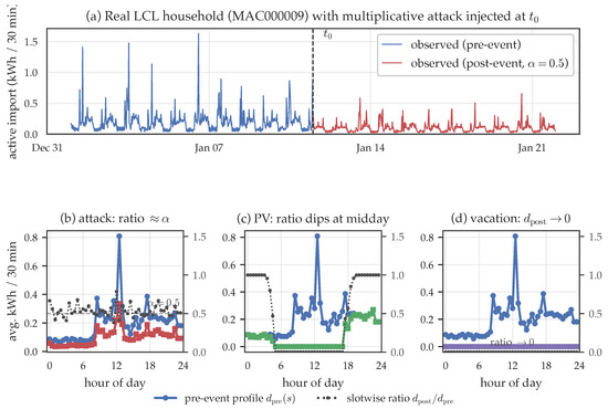
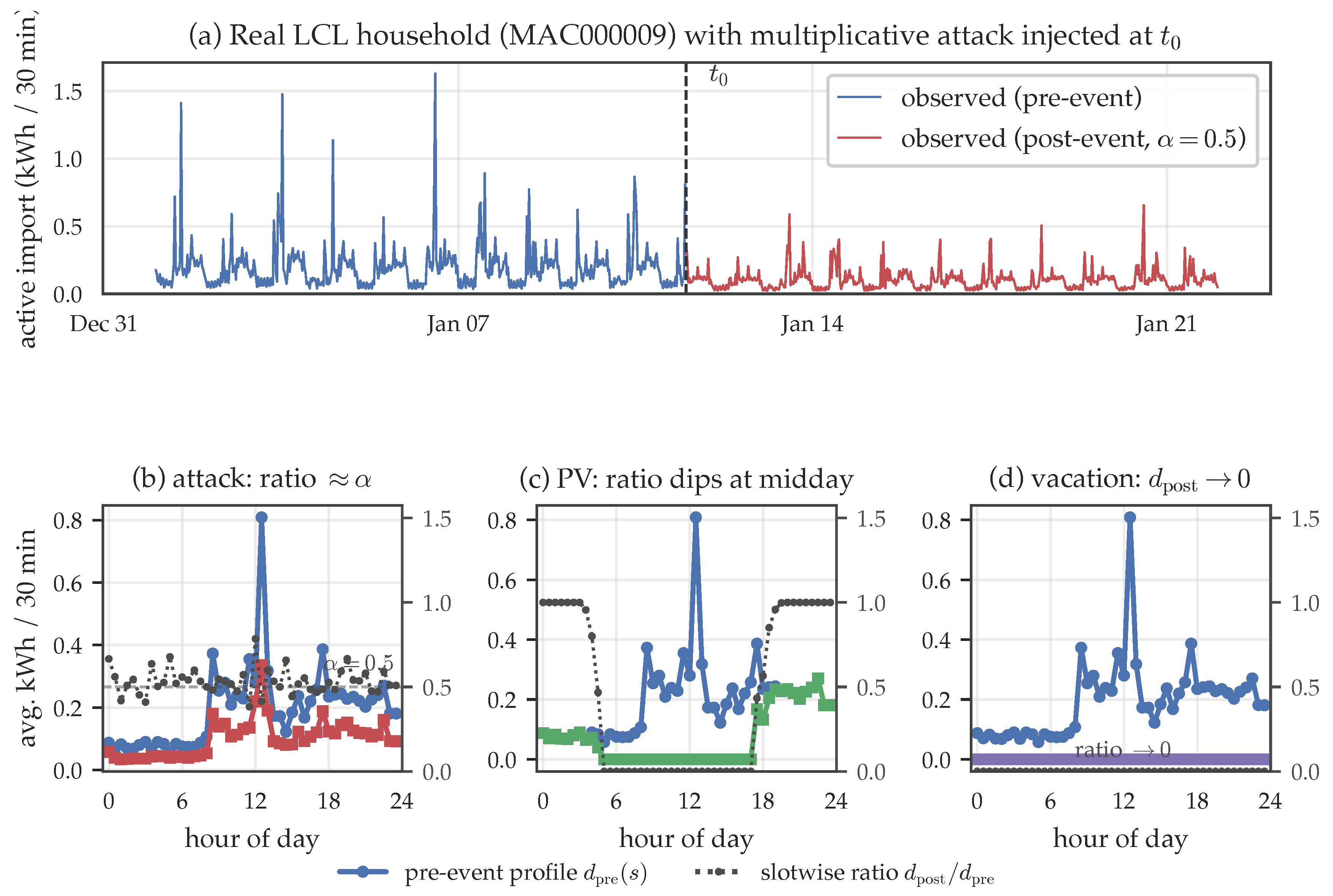
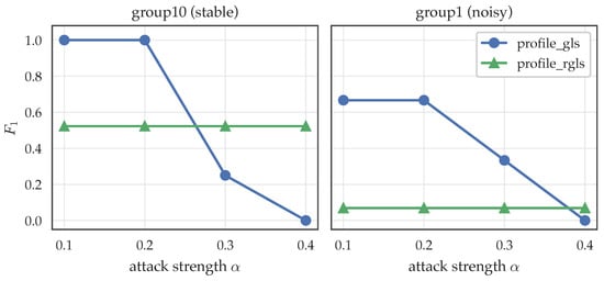
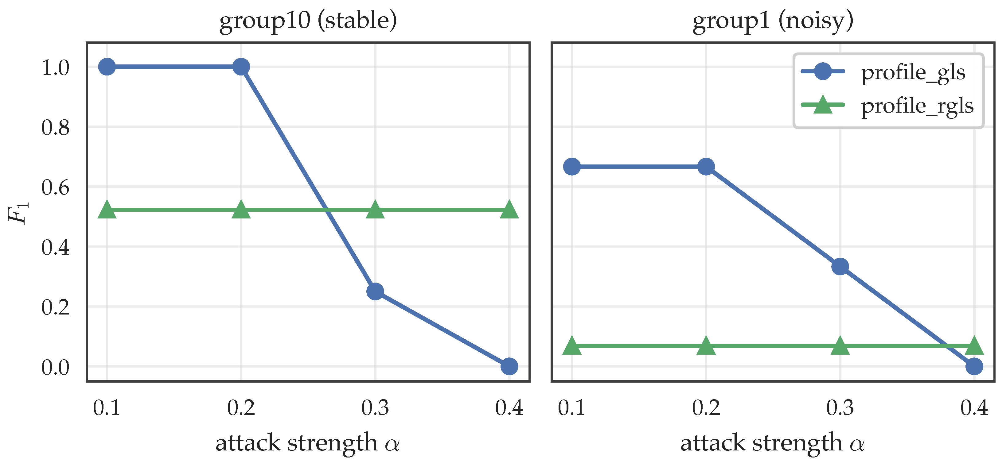
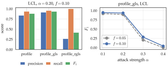
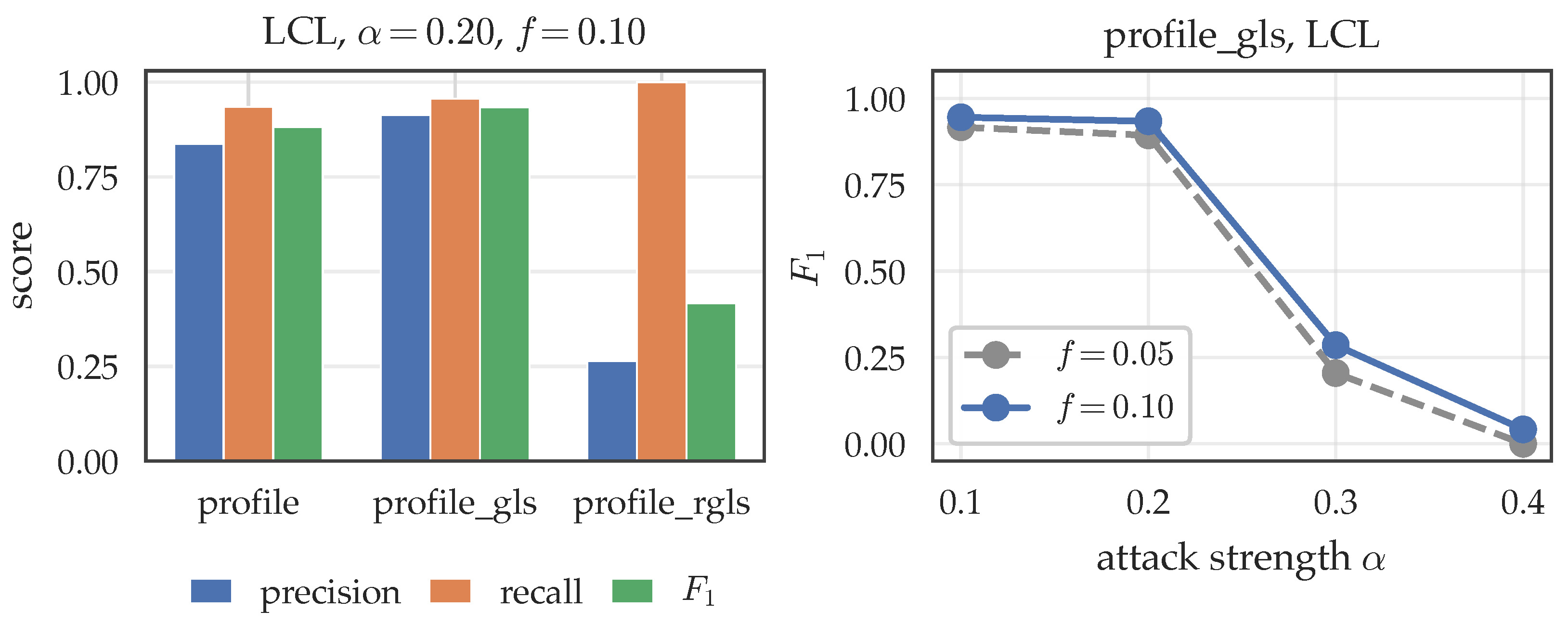
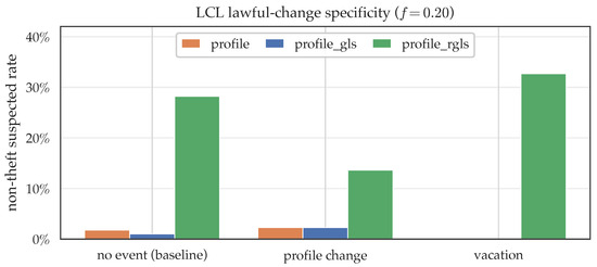
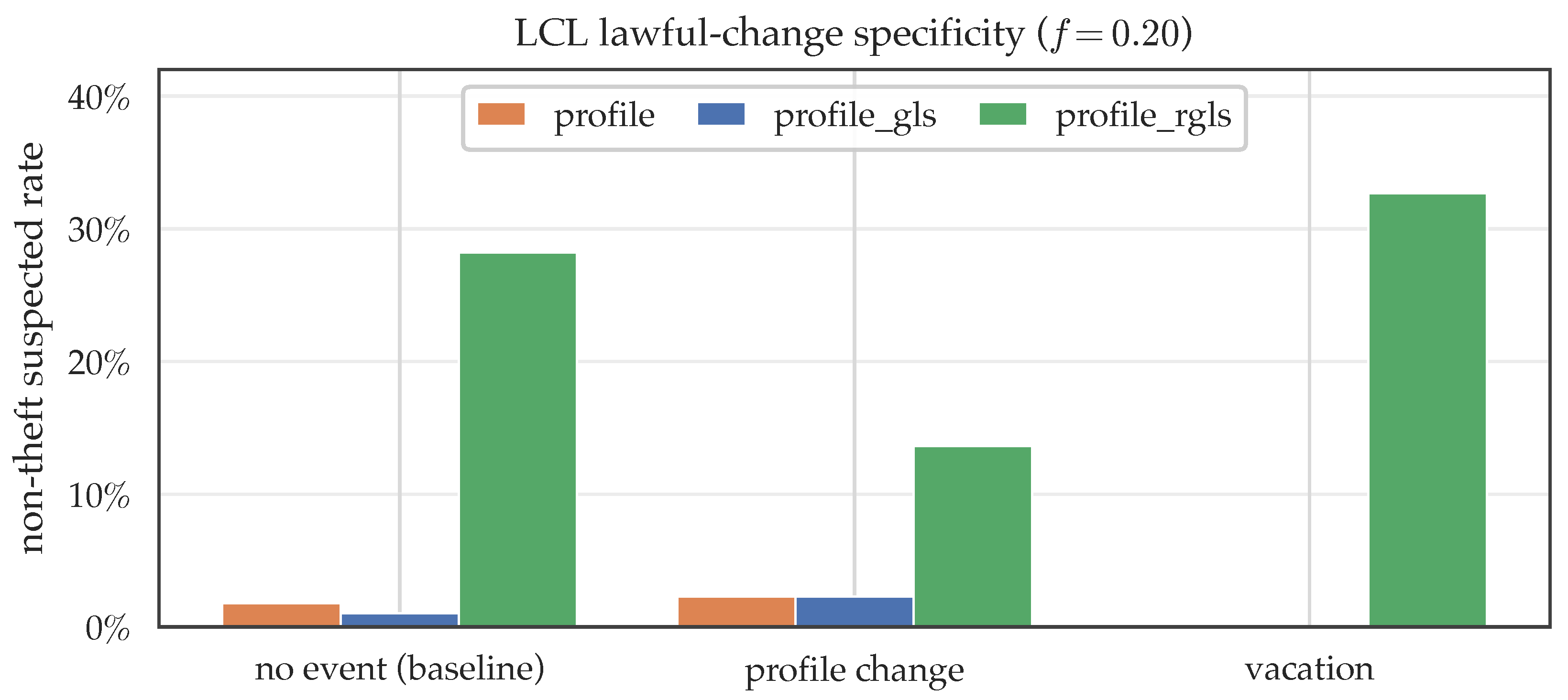
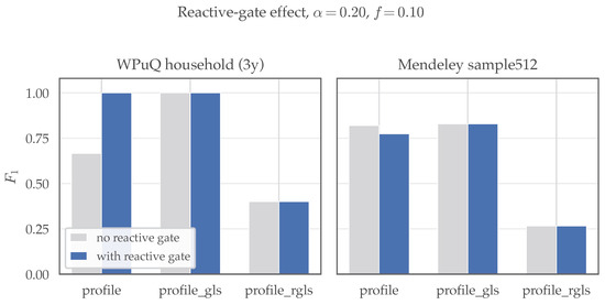
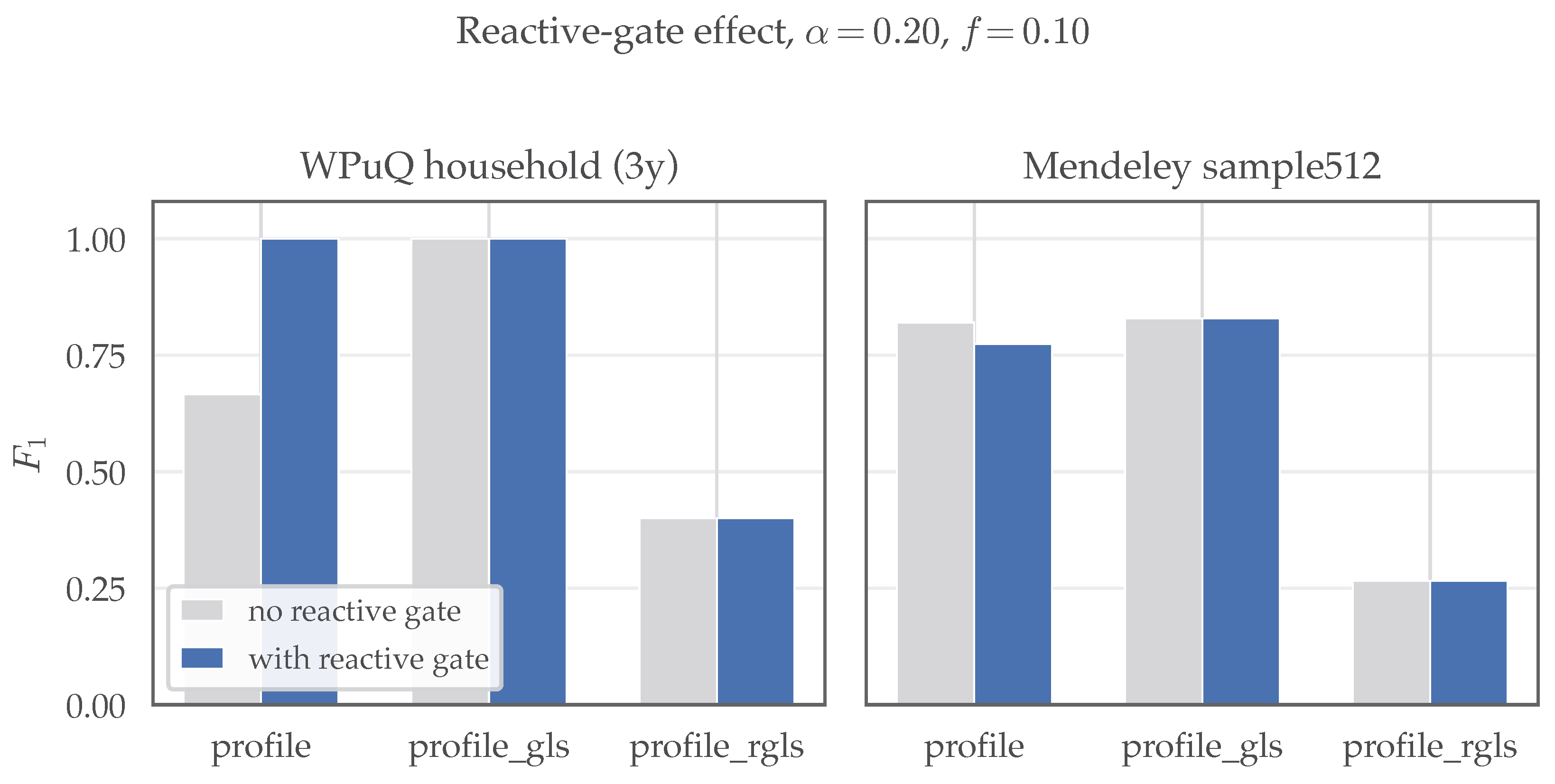
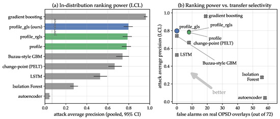
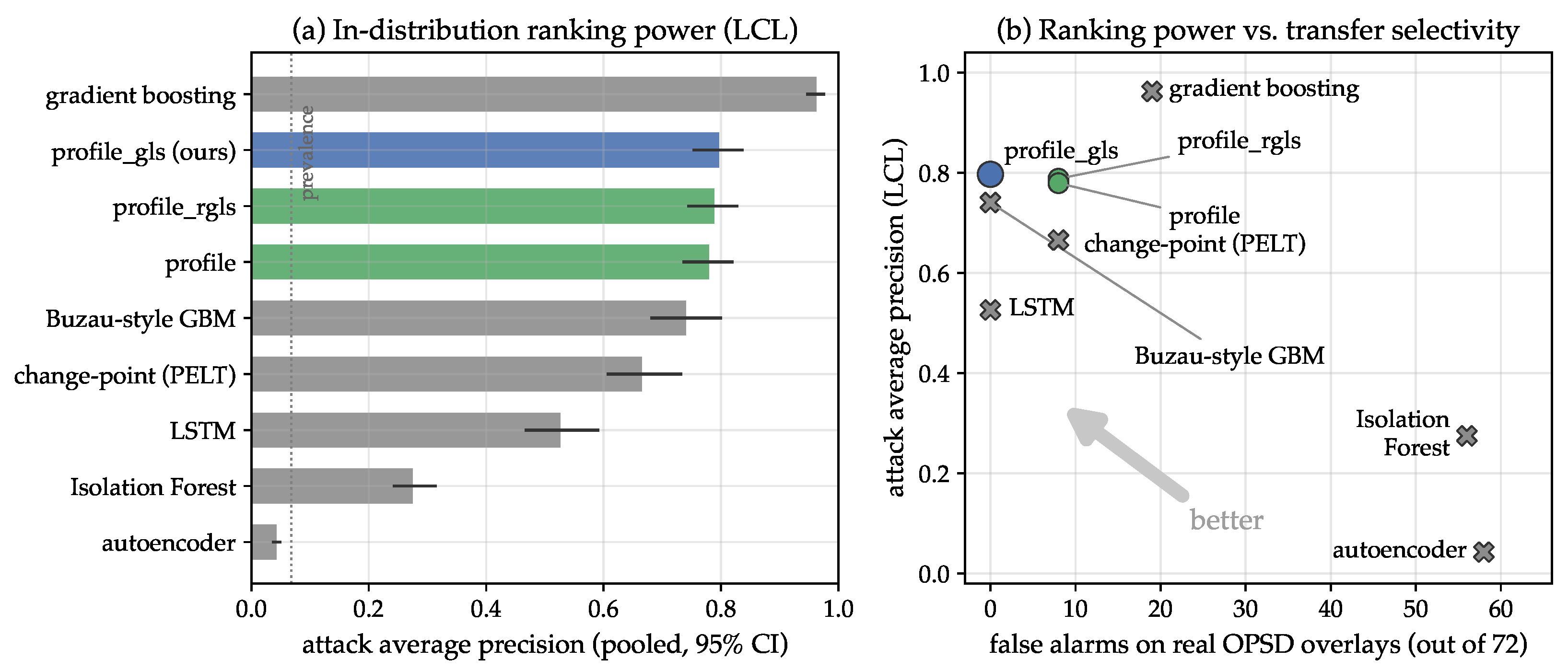
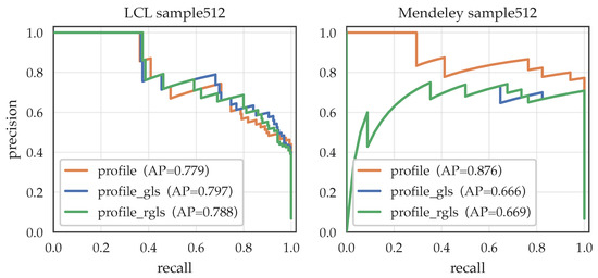
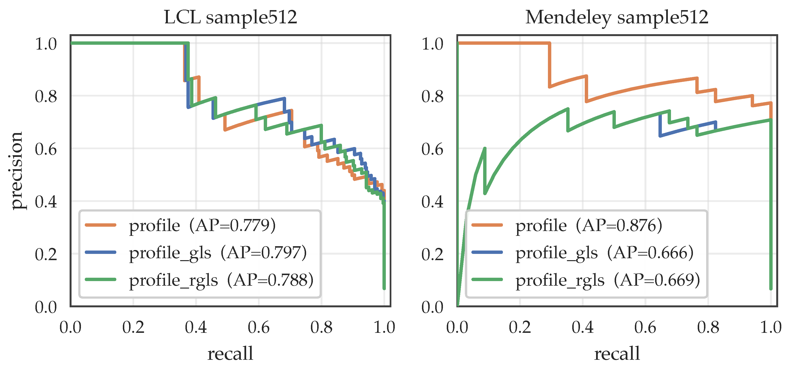
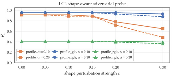
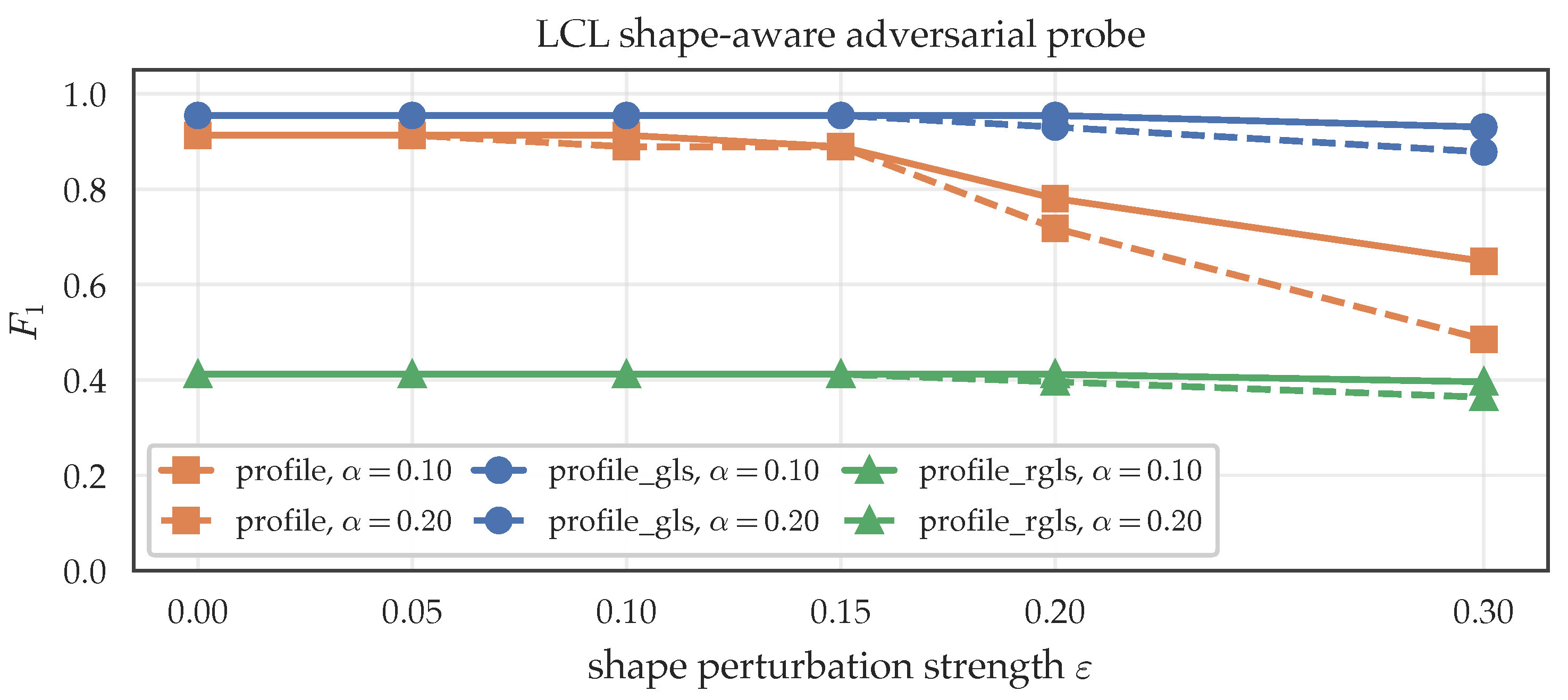
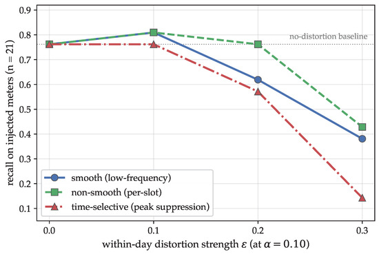
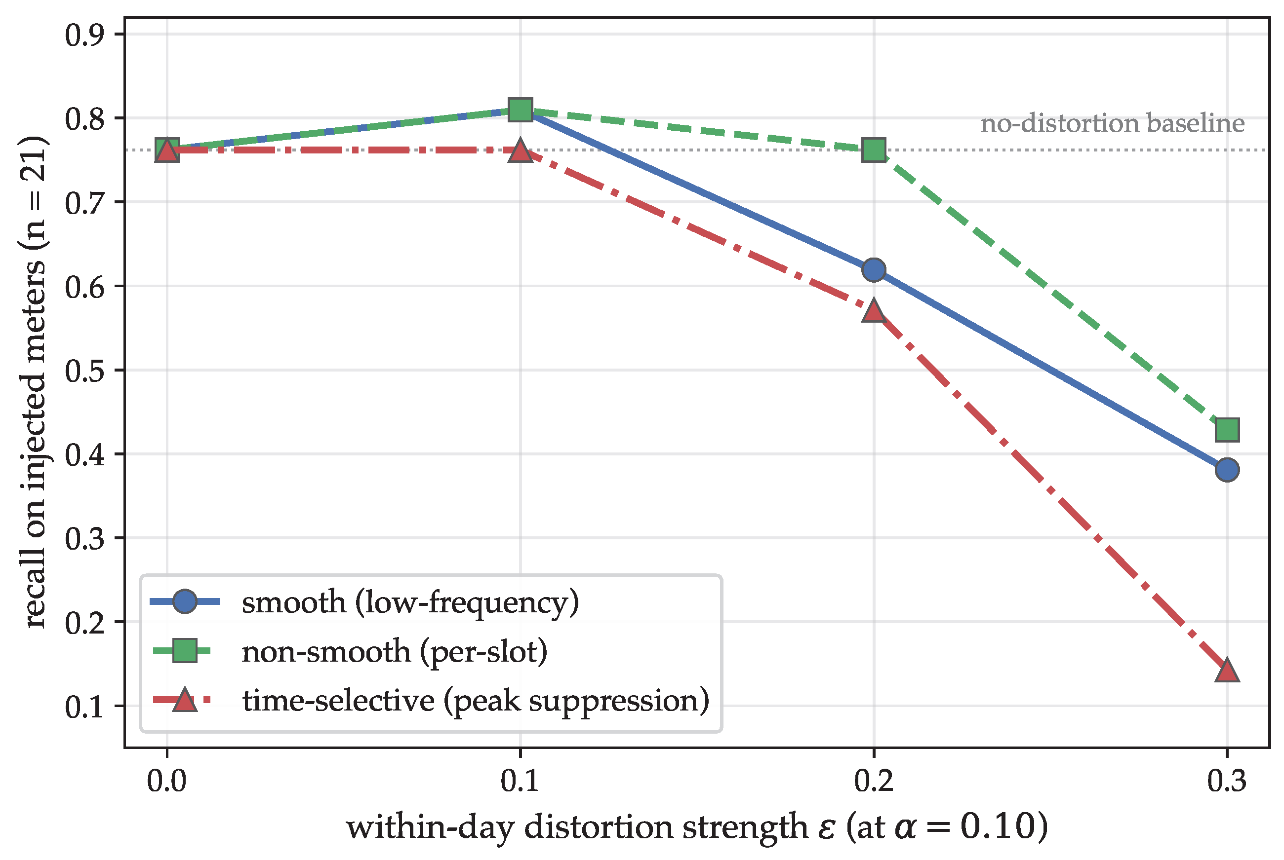

Disclaimer/Publisher’s Note: The statements, opinions and data contained in all publications are solely those of the individual author(s) and contributor(s) and not of MDPI and/or the editor(s). MDPI and/or the editor(s) disclaim responsibility for any injury to people or property resulting from any ideas, methods, instructions or products referred to in the content. |
© 2026 by the author. Licensee MDPI, Basel, Switzerland. This article is an open access article distributed under the terms and conditions of the Creative Commons Attribution (CC BY) license.