Universal Robust Vehicle Identification System for Monitoring Using YOLOv12 and DeepSORT

Highlights

What are the main findings?

• A semi-automated synthetic dataset generation technique significantly reduced manual annotation requirements while improving model robustness across varying camera viewpoints.
• The integrated YOLOv12–DeepSORT framework achieved 96.67% accuracy for vehicle counting, 90% for seven-category vehicle-type prediction, and up to 97% for public/private vehicle class prediction.

What are the implications of the main findings?

• The universal approach enables system application across different locations without extensive location-specific retraining.
• The system demonstrates feasibility for deployment in real-world intelligent transportation systems for traffic monitoring and policy formulation in the Philippines.

Abstract

Persistent traffic congestion and the need for efficient traffic monitoring have increased the demand for automated vehicle-analysis systems based on CCTV footage. This study presents a CCTV-based vehicle monitoring system that integrates vehicle detection, tracking, counting, public/private vehicle class prediction, seven-category vehicle-type prediction, vehicle-color recognition, and traffic-state estimation using YOLOv12 and DeepSORT. To reduce manual annotation effort during the initial training stage, a semi-automated method for generating synthetic composite road scenes was developed by combining cropped vehicle images and road-background images. The detector was first trained on 10,000 synthetic images and then sequentially fine-tuned on real CCTV data. Four real-world traffic video clips from Metro Manila were used in the study. Three 5 min clips were used within the staged refinement workflow: the first two for iterative refinement and the third for final post-refinement evaluation of the adapted model. A separate fourth CCTV clip was reserved exclusively for blind evaluation without on-the-fly retraining. The final system achieved average accuracies of 97% for public/private vehicle class prediction, 90% for seven-category vehicle-type prediction, 82% for vehicle-color recognition, and 96.67% for vehicle counting on the final evaluation video. The results show that synthetic pretraining combined with limited real-world fine-tuning can improve performance in CCTV-based vehicle monitoring while reducing the amount of manually labeled real-world data required. The study also discusses the limitations of the current evaluation protocol and the need for broader multi-location testing.

1. Introduction

Metro Manila’s major issue is traffic congestion. Persistent delays continue to affect mobility, productivity, and traffic management. According to the 2025 TomTom Traffic Index for Manila, the metropolitan area recorded an average congestion level of 57%, an average travel time of 31 min 45 s for a 10 km trip, and 143 h of time lost during rush hour over the year. These conditions motivate the need for scalable and automated vehicle-monitoring systems that can operate on existing CCTV infrastructure.

Numerous studies have applied image processing and machine learning for vehicle detection and classification. Approaches such as Faster R-CNN, SSD (Single-Shot Detector), and YOLO (You Only Look Once) have demonstrated varying degrees of accuracy in object detection tasks. Prior work typically focuses on one or two specific features—such as vehicle classification, color recognition, or traffic flow estimation—but rarely integrates all these capabilities into a single comprehensive system. For instance, ref. [1] developed a CNN-based system that quantifies vehicles and classifies them as public or private (with subcategories), but it did not incorporate color detection or traffic congestion level estimation. Ref. [2] achieved vehicle color recognition using histogram back-projection and SVM, but did not classify vehicle types or count vehicles. Other researchers have addressed vehicle brand recognition [3], license plate recognition and speed estimation [4,5], multi-camera vehicle identification [6], and toll classification using ensemble classifiers [7]. Some have achieved very high accuracy for their specific tasks—e.g., ref. [7] reported 99.03% for vehicle type classification, and methods like DenseNet-CMP [8] have achieved 98% accuracy in fine-grained model classification. However, these studies typically do not combine all functionalities (counting, class, type, color detection, and traffic state recognition) into a single system. Moreover, many systems are trained and tested on particular datasets (sometimes from limited viewpoints or specific locations) and may not generalize well to new environments without retraining.

Recent studies have shown that synthetic and hybrid real–synthetic datasets can improve object-detection performance when manually labeled real data are limited, although these approaches remain subject to domain-gap and realism constraints [9,10]. Accordingly, the contribution of the present study is not the concept of synthetic data itself, but a practical and low-cost composite-data workflow tailored to fixed CCTV intersections, coupled with staged refinement on limited real-world footage and integrated deployment for vehicle detection, tracking, counting, color attribution, and traffic-state estimation. While prior traffic-monitoring studies have combined detection, classification, or tracking modules in various ways, the contribution of the present work lies in the specific integration strategy adopted for fixed CCTV surveillance. First, the study uses a low-cost semi-automated compositing workflow to generate scene-aware synthetic training images that reduce the dependence on extensive manual annotation. Second, the detector is refined through staged adaptation on limited real CCTV footage rather than being retrained from scratch for each deployment scenario. Third, the resulting system combines vehicle detection, tracking, counting, local vehicle categorization, color attribution, and traffic-state estimation in a single operational pipeline designed for practical traffic monitoring under the tested conditions.

More recent literature has continued to explore both integrated detection–tracking pipelines and improved detection backbones for intelligent traffic monitoring. For example, recent work has examined YOLO–DeepSORT integration for real-time vehicle detection and tracking, improved YOLOv5s–DeepSORT variants for better detection and tracking robustness, and broader deep-learning-based tracking pipelines for intelligent transportation surveillance. In parallel, recent reviews have emphasized the importance of standardized datasets, evaluation metrics, and deployment-oriented benchmarks in traffic-monitoring research. These developments position the present work within an active research area focused not only on detection accuracy, but also on adaptation, operational robustness, and deployment practicality [11,12,13,14].

This paper aims to address these gaps by developing a robust CCTV-based vehicle monitoring system capable of vehicle detection, tracking, counting, classification (public vs. private and further by vehicle category), color recognition, and traffic-state estimation from video feeds. The proposed system leverages YOLOv12 for object detection and DeepSORT for multi-object tracking, creating a pipeline that can tag and follow multiple vehicles in real time. A semi-automated synthetic-data generation workflow is used to reduce manual labeling effort during initial model development, after which the detector is refined using limited real-world CCTV footage. In this way, the study focuses on practical staged adaptation and integrated deployment rather than treating synthetic-data usage or object tracking alone as the main novelty. Throughout this paper, vehicle class refers to the binary public/private grouping, vehicle type refers to the seven-category detector taxonomy, and vehicle color refers to the auxiliary attribute-recognition task.

2. Materials and Methods

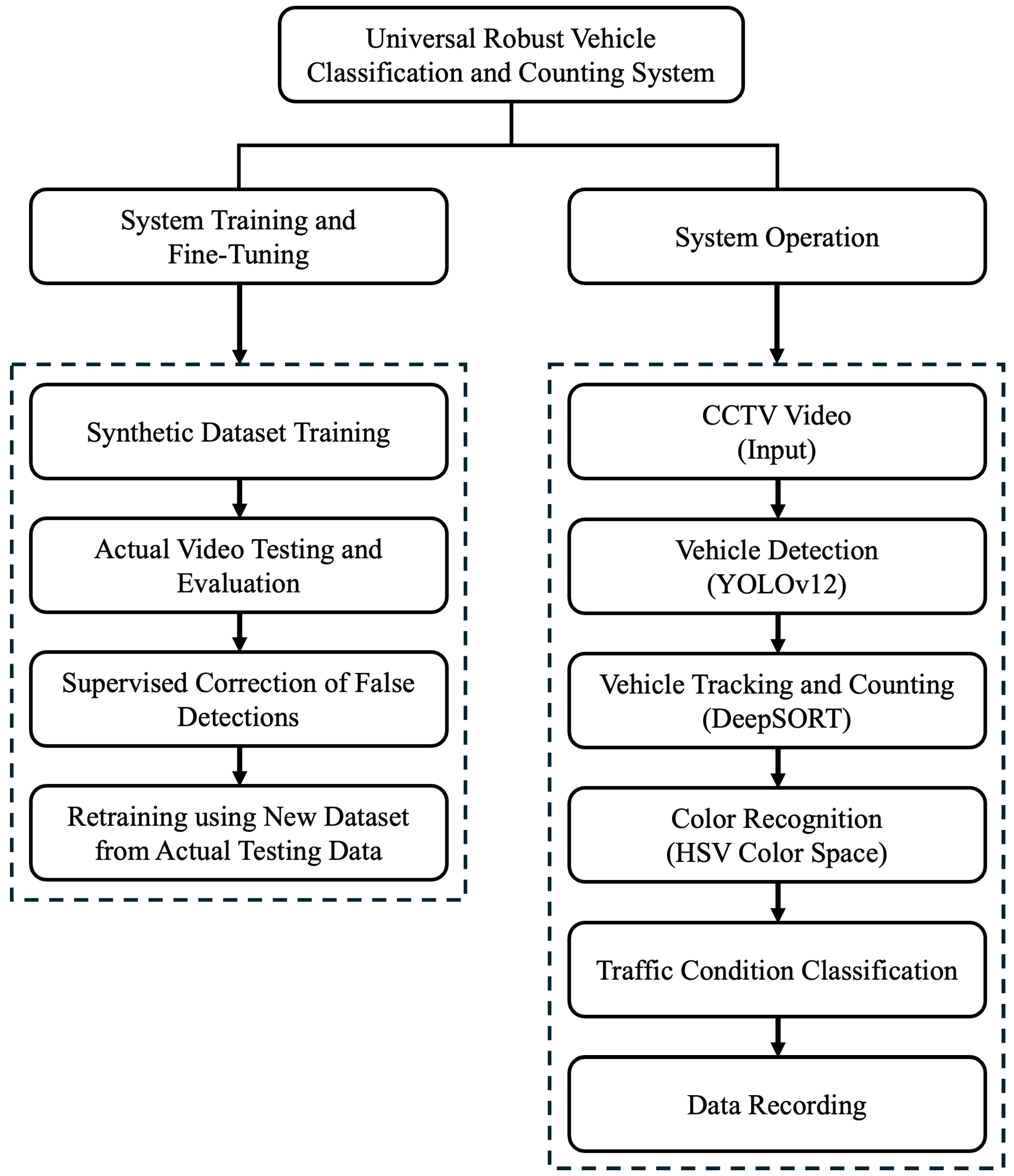
Figure 1 shows the overall system architecture of the proposed vehicle monitoring system. The system consists of two main stages. The first stage focuses on detector development, including synthetic-data generation, initial training, and staged real-world refinement. The second stage focuses on deployment, in which the trained model processes CCTV video frame by frame using YOLOv12 for vehicle detection, DeepSORT for tracking and counting, HSV-based color attribution, and rule-based traffic-state estimation.

2.1. System Training and Fine-Tuning

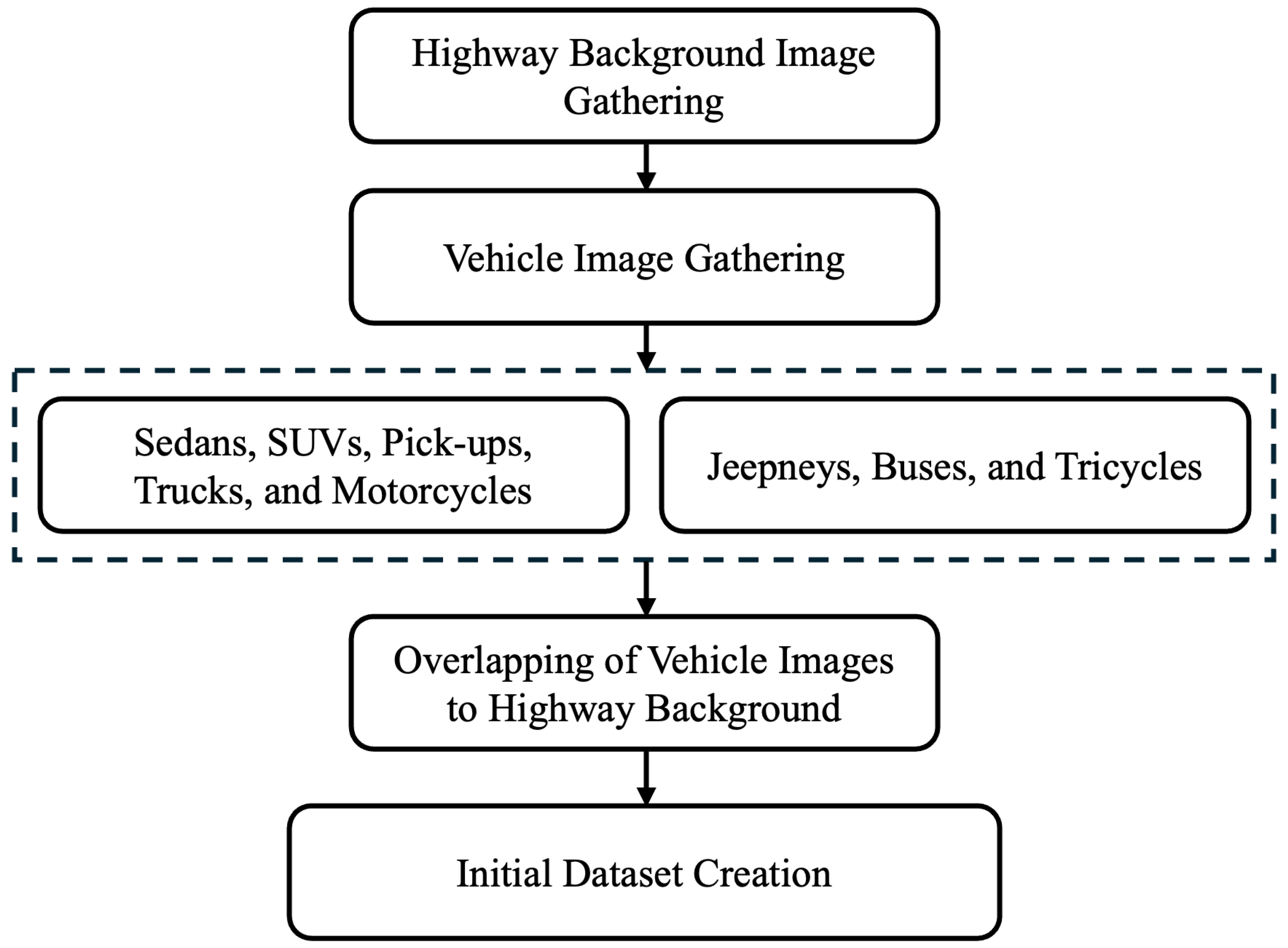
One of the primary difficulties in building reliable detection models is the requirement for extensive, varied, and well-annotated datasets. To minimize the labor-intensive process of manually capturing and labeling thousands of images across different environments and camera viewpoints, we adopted a semi-automated data generation approach, illustrated in Figure 2. This method involved compiling sets of vehicle images and background road scenes—such as empty streets, intersections, and highways—and combining them to produce synthetic training samples. Through this process, we were able to emulate traffic scenes corresponding to specific intersections, camera placements, object scales, and vehicle orientations.

The vehicle images were carefully selected from online datasets and original photographs and represented seven target categories: (1) sedans, (2) sport utility vehicles (SUVs), (3) trucks (including 8-wheeler trucks), (4) motorcycles, (5) passenger utility jeepneys (PUJs), (6) tricycles (motorcycles with sidecars), and (7) buses, captured from multiple viewpoints such as front, rear, side, and angled perspectives. These vehicle images were either segmented to remove their backgrounds or sourced with transparent backgrounds. Road background images were collected from diverse locations and viewing angles, including screenshots from publicly accessible traffic cameras when available.

A major challenge in developing robust detection models is the need for large, diverse, and annotated datasets. To reduce the manual effort of collecting and labeling thousands of images covering various scenes and camera angles, we implemented a semi-automated data generation process as shown in Figure 2. We gathered collections of vehicle and background images (empty road scenes, intersections, highways) and overlapped them to create composite training images. This technique allowed us to simulate scenes appearing in specific intersections, camera positions, scales, and vehicle orientations on roads.

Prior to composite-image generation, the background road images and cropped vehicle images were organized into separate directories. The background images were stored in one folder, while the vehicle crops were grouped first by vehicle class and then by orientation. For each vehicle class, eight orientation folders were used: north, south, east, west, northeast, northwest, southeast, and southwest. To increase appearance diversity, scripts were used to generate additional color variants for motorcycles, sedans, trucks, and SUVs. For PUJs, buses, and tricycles; separate scripts were used to generate additional color and side-pattern variations representative of public-transport paint schemes.

During composition, the lane geometry of each selected background image constrained the admissible vehicle positions, scales, and orientations. Vehicle centroids were placed stochastically along lane-specific centerlines, and the crop scale was sampled within bounds determined by lane width and expected perspective. In addition to the compositing procedure itself, standard YOLO training augmentations were applied during detector training. Dedicated simulation of weather, motion blur, or sensor noise was not explicitly performed in the present study. Instead, the domain gap between synthetic and real imagery was mitigated primarily through staged refinement on manually reviewed and corrected CCTV-derived frames.

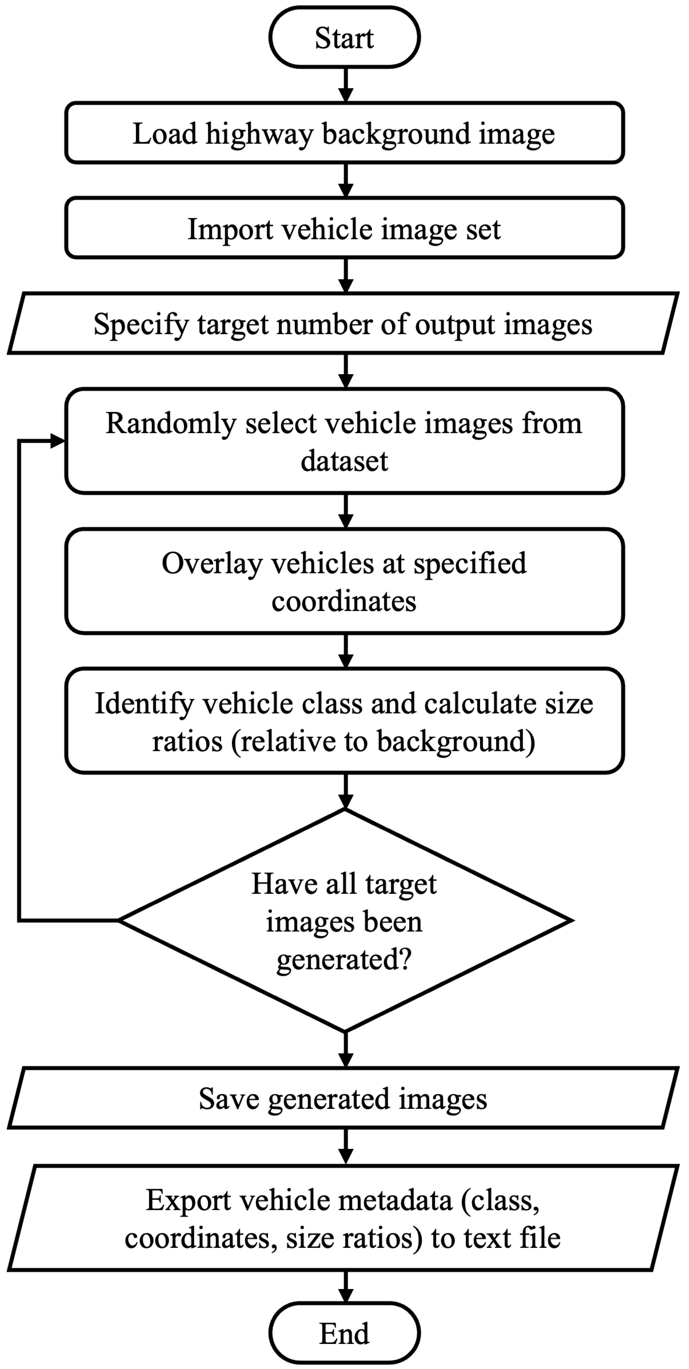
A key step in the synthetic-data pipeline is the placement of appropriately scaled vehicle crops onto each background scene. For each lane, the lane width, usable lane length, and traffic-flow direction were specified in advance. These parameters determined which orientation-specific vehicle folders could be sampled, the allowable scale of each crop, and the maximum number of vehicles that could be placed in the lane. The user also specified the target number of output images and the destination directory. Figure 3 summarizes the dataset-generation workflow.

A Python-based script was created to automatically fill a pre-selected appropriate background image—matched closely to the intended deployment environment—and randomly choose vehicle images according to the traffic direction and volume in each lane. These vehicles are then overlaid onto the road background at randomized locations. For every synthesized image, the script automatically logs the bounding box coordinates and corresponding class labels of all inserted vehicles into an annotation file formatted for YOLO. Vehicle dimensions are adjusted proportionally based on the width and length of the lane in which they are placed. In addition, the script generates a lane-specific centerline following the traffic flow, which serves as a reference for positioning the centroids of the resized vehicle images.

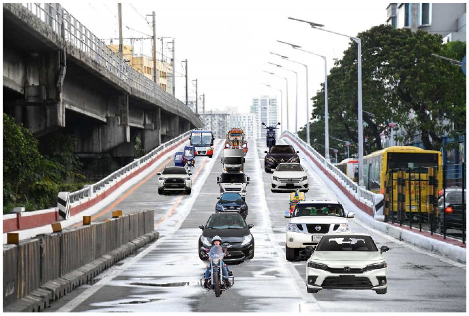
The placement of vehicles is randomized based on their source classification directories and the maximum number of vehicles assignable per lane. Each lane may contain one or multiple vehicles, potentially belonging to different categories, ensuring a high degree of variability. This randomized procedure produces diverse and non-repetitive training samples and automatically terminates once the user-specified number of images has been generated. Sample composite images produced through this process are shown in Figure 4. Overall, this method resembles data augmentation techniques and enables the model to acquire prior knowledge of a wide range of vehicle appearances without the need to manually annotate every training image.

We curated 10,000 synthetic images for initial training. We split the synthetic dataset into 80% for training and 20% for validation. Using the YOLOv12 training framework, we initially trained the model on this dataset for 10 epochs. The training process used stochastic gradient descent (SGD), and standard data augmentation was included in YOLOv12 (random scaling, mosaic image combinations, etc.). After training, the model’s performance on the validation set was evaluated via a confusion matrix for the seven vehicle classes.

To improve reproducibility, the training configuration of the YOLOv12 detector is summarized here. The detector input was resized to $640\times 640$ pixels. For the reported initial synthetic-data training run, the model was trained using stochastic gradient descent (SGD) with an initial learning rate of ${10}^{-2}$, a batch size of 16, and 10 epochs. Standard YOLO augmentation strategies were enabled during training, including HSV-based color perturbation, rotation, translation, scaling, shear, perspective transformation, flipping, mosaic augmentation, and mixup. The experiments were conducted using Python 3.12.3 and PyTorch 2.6.0 on an NVIDIA RTX 2070 GPU. The settings are tabulated in

Table 1. YOLOv12 training configuration used in this study.

Parameter	Setting
Input size	$640\times 640$
Optimizer	SGD
Initial learning rate	${10}^{-2}$
Batch size	16
Initial training epochs	10
Augmentations	HSV hue/saturation/value adjustment; rotation; translation; scaling; shear; perspective transformation; flipping; mosaic; mixup
Framework	Python 3.12.3, PyTorch 2.6.0
Hardware	NVIDIA RTX 2070

.

The class distribution of the synthetic dataset was controlled to ensure representation of all seven vehicle categories used in the study. However, the distribution was not perfectly uniform, and classes with fewer source images—particularly buses and trucks—remained relatively less represented, which may partly explain the weaker performance observed for those categories during evaluation. This issue is discussed further in the Results and Limitations sections.

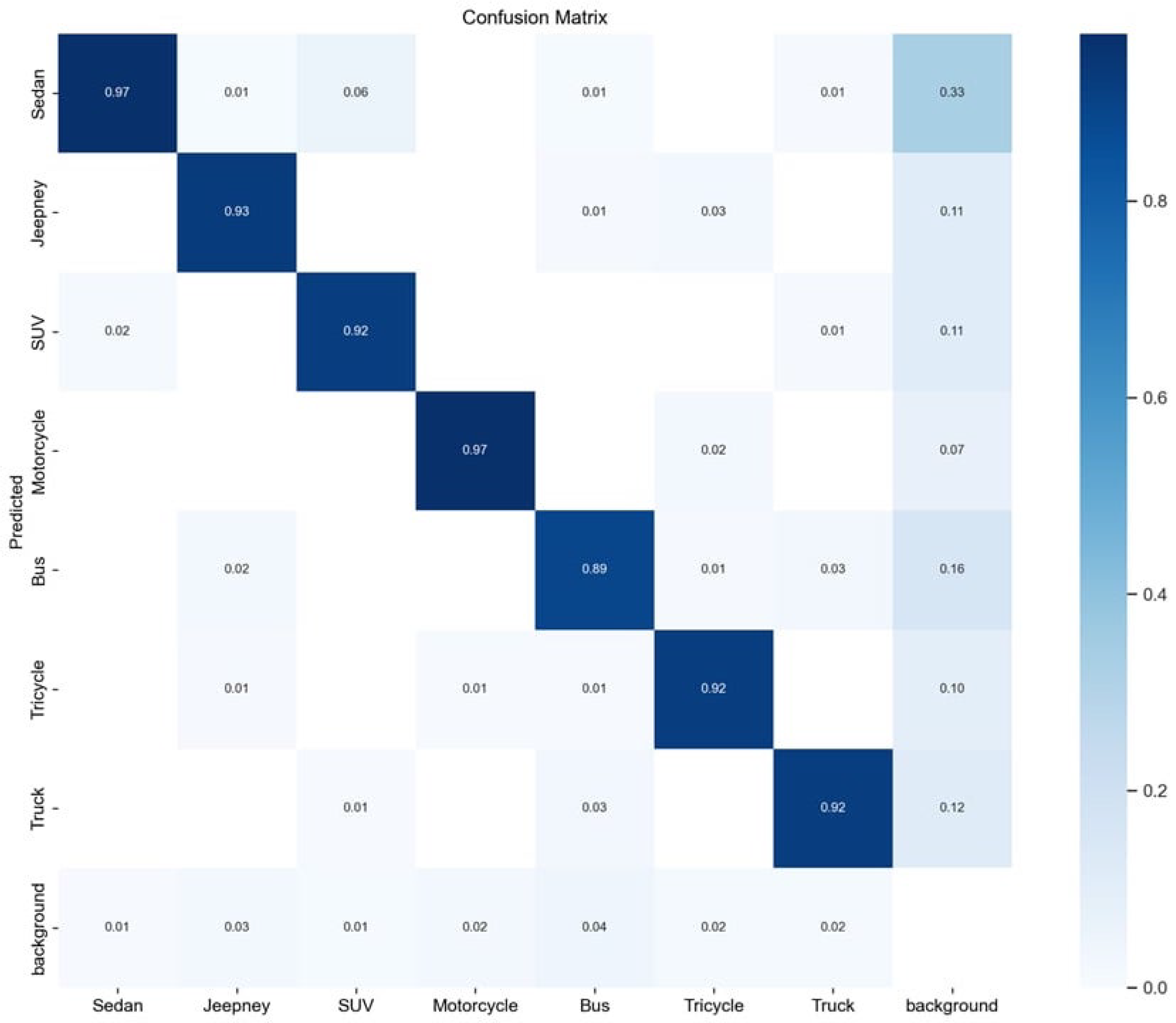
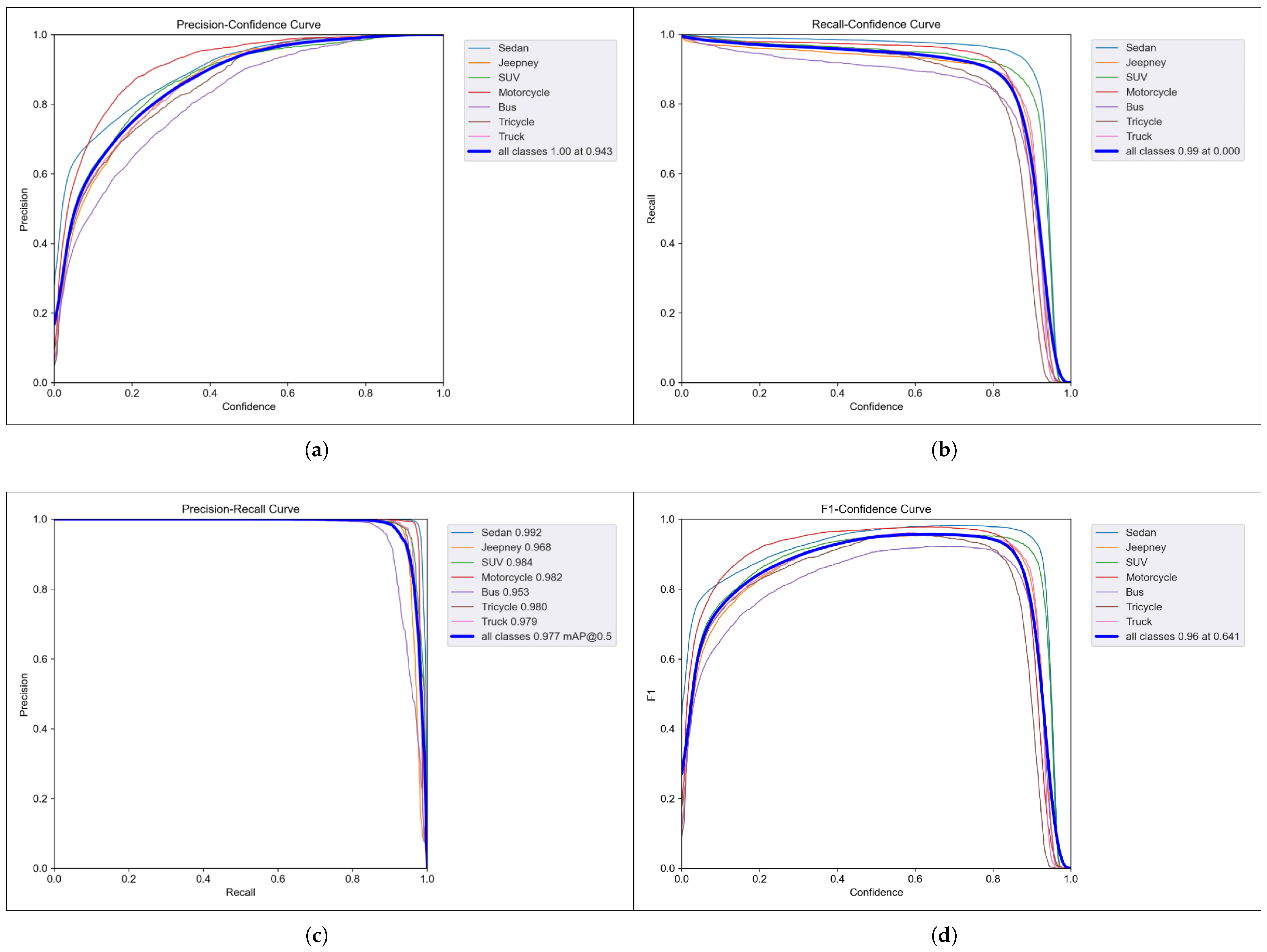
Figure 5 shows the normalized confusion matrix obtained on the synthetic validation split after the initial training stage. This result reflects in-domain performance on the generated dataset only and is intended to verify that the detector learned the target classes before real-world adaptation. It should not be interpreted as the final field evaluation. The detector was further evaluated on the synthetic validation split using precision–recall analysis. The resulting mean average precision at an IoU threshold of 0.5 was 0.977 across all classes. The class-wise AP@0.5 values were 0.992 for sedan, 0.968 for jeepney, 0.984 for SUV, 0.982 for motorcycle, 0.953 for bus, 0.980 for tricycle, and 0.979 for truck. In addition, the overall maximum F1 score reached 0.96 at a confidence threshold of 0.641. The precision–confidence, recall–confidence, precision–recall, and F1–confidence curves are shown in Figure 6. Real-world performance was assessed separately using manually reviewed CCTV videos, as reported later in the succeeding sections.

Model Fine-Tuning with Real-World Data

Although the initial model successfully learned general vehicle detection and classification, it revealed noticeable domain mismatches when evaluated on real-world CCTV footage (Video 1; see Section 3). In particular, vehicles located farther from the camera—appearing smaller in scale—were occasionally undetected, and some instances of misclassification were observed. The most frequent error involved pickup trucks being incorrectly labeled as SUVs due to their similar visual characteristics. To address these limitations and enhance overall performance, we employed an iterative fine-tuning approach.

To enhance model performance, we employed an iterative fine-tuning approach. First, the trained model was applied to a five-minute CCTV recording (Video 1) captured from a Metro Manila traffic monitoring system along an urban highway with a designated bus lane. The model produced an annotated video and a detection log. From this footage, frames were extracted at a rate of six frames per second, resulting in approximately 1800 unique images. These frames were manually examined by comparing the model’s predicted vehicle classes and colors against the original footage.

Cases of incorrect classification and missed detections were documented. For recurring error patterns—such as the failure to detect vehicles at greater distances—a subset of affected frames was manually relabeled to correct the annotations. These corrected frames were then incorporated into an expanded training dataset, effectively treating them as new labeled examples that captured the model’s weaknesses.

Using this augmented dataset, the YOLOv12 model was further trained for several additional epochs. The new real-world samples were combined with the original set of 10,000 synthetic images to mitigate catastrophic forgetting, resulting in an updated version of Model 1.

The refined model was subsequently evaluated on another five-minute CCTV clip recorded on the same day (Video 2). The same workflow was applied: detections were logged, errors were reviewed—now notably reduced—misclassified frames were corrected, and these new samples were added to the training pool. Another round of fine-tuning yielded Model 2.

Finally, Model 2 was tested on a third video (Video 3), where it achieved the desired performance level, with key metrics reaching approximately 90% or higher. At this stage, the iterative fine-tuning process was concluded.

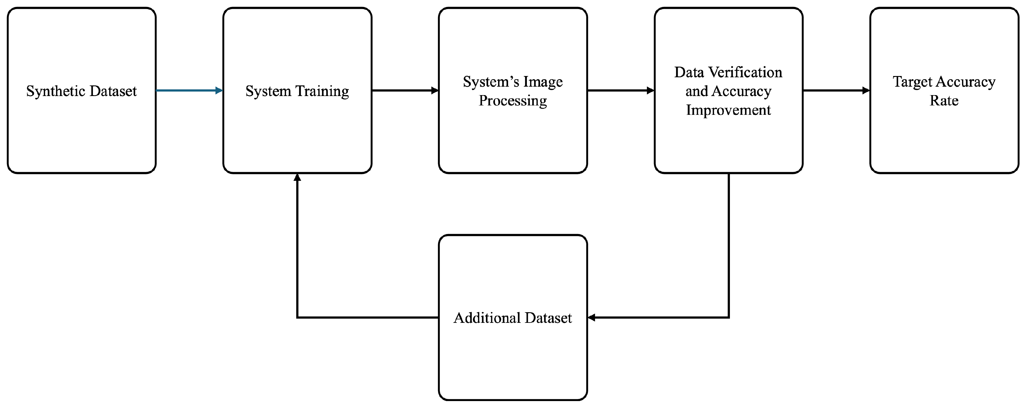
This fine-tuning approach is illustrated in Figure 7. It allowed the model to incrementally learn from its mistakes and adapt to the actual camera perspectives and environmental conditions in our target deployment, without having to retrain from scratch for each new video. Each fine-tuning round used a relatively small number of additional images (around 1800 frames per round, since not every frame of the videos was used) and a limited number of epochs (5–10) to avoid overfitting to the latest video. We maintained a separate validation set to ensure the model’s improvements generalized beyond the exact video it had seen. Each iteration refines the model, yielding progressively higher accuracy on real data.

To avoid ambiguity regarding the evaluation protocol, we clarify that the present study used a staged adaptation design. The synthetic dataset was used only for initial training and validation. Videos 1 and 2 were then used as development videos for real-world error analysis and iterative fine-tuning under actual CCTV conditions. Finally, Video 3 was used as a post-refinement evaluation video. Accordingly, the present work should be interpreted as a staged feasibility study for real-world adaptation rather than a large-scale no-retraining benchmark across many unseen sites.

All three real-world CCTV videos were obtained from Metro Manila traffic surveillance feeds and were processed at a resolution of $1280\times 720$. The videos depict a similar urban highway corridor with a bus lane under fair daylight conditions; the key differences are their role in the staged evaluation protocol and the traffic conditions observed during each clip. A summary is placed in

Table 2. Summary of the real-world CCTV videos used in the study.

Video	Duration	Time of Day	Traffic Density	Reference Vehicles	Role in Study
Video 1	5 min	Morning	Common lanes: heavy; bus lane: light	Not explicitly reported	First real-world refinement round
Video 2	5 min	Noon	Common lanes: heavy; bus lane: light	Not explicitly reported	Second real-world refinement round
Video 3	5 min	Afternoon	Common lanes: heavy; bus lane: light	300	Final post-refinement evaluation

.

Where directly measured metadata such as exact source-feed weather labels or the number of unique/reference vehicles were not available, approximate scene descriptions based on manual review were used instead. Accordingly, this table is intended to clarify the experimental context rather than to claim a fully standardized benchmark dataset.

2.2. Blind Evaluation Protocol

To address potential information leakage between model development and final evaluation, an additional blind evaluation protocol was defined using a separate fourth CCTV video clip that was not part of the staged refinement workflow described earlier. This blind test video was reserved exclusively for testing and was not used for training, annotation correction, threshold adjustment, hyperparameter selection, or further fine-tuning. Two model states were considered for comparison: (1) a zero-shot model trained only on the synthetic dataset, and (2) an adapted model obtained after refinement using Videos 1 and 2 only. Both model states were frozen prior to blind evaluation, and the blind test video was used only once for final performance measurement.

The blind CCTV clip was obtained from the same general Metro Manila traffic-surveillance context as the other evaluated videos, but it was excluded from all development-stage adaptation steps. As in the previous real-world evaluations, performance on the blind clip was determined through manual review of the processed video outputs, using the same prediction levels reported in this study: public/private vehicle class, seven-category vehicle type, vehicle color, and vehicle counting accuracy.

This protocol is intended to complement the staged refinement results reported earlier in the paper. Accordingly, the blind-study results should be interpreted as an evaluation without on-the-fly retraining, whereas the previously reported Video 1–Video 3 results represent the staged adaptation workflow used to develop the system.

2.3. System Operation

For clarity, the online processing workflow of the proposed system can be summarized as follows:

• Read the input CCTV video and extract frames sequentially.
• Apply YOLOv12 to each frame to generate vehicle detections and class probabilities.
• Perform non-maximum suppression to remove duplicate overlapping detections.
• Pass the filtered detections to DeepSORT for track initialization, ID assignment, and track updating across frames.
• Evaluate track centroids against the predefined counting lines or ROIs to update lane-wise and total vehicle counts.
• Extract each detected vehicle region and assign a color label using the HSV-based rule set.
• Aggregate recent vehicle-count trends over the defined time window and estimate the traffic state for each lane and for the full scene.
• Render the output annotations and write the detection, tracking, counting, and summary results to the output video and log files.

For formal clarity, let $I_t$ denote the input frame at time step t. The YOLOv12 detector $D_{\theta }$ maps $I_t$ to a set of detections

$${\mathcal{Y}}_t=D_{\theta }\left(I_t\right)={\left\{(b_i^t,{\widehat{y}}_i^t,s_i^t)\right\}}_{i=1}^{N_t},$$

where $b_i^t$ is the predicted bounding box, ${\widehat{y}}_i^t$ is the predicted vehicle type, and $s_i^t$ is the confidence score of the ith detection. After non-maximum suppression, the filtered detections are passed to the DeepSORT tracker T, which updates the active trajectory set

$${\mathcal{T}}_t=T({\mathcal{T}}_{t-1},{\mathcal{Y}}_t),$$

where each trajectory is associated with a persistent track ID across frames.

For each active track k, let $g_k^t$ denote the centroid of its bounding box at time t. A counting event is registered for lane or region m when $g_k^t$ crosses the corresponding counting line $L_m$, in which case the count variable $C_m$ is incremented. Vehicle class is defined as a binary super-category derived from vehicle type through the mapping

$$\varphi \left({\widehat{y}}_k^t\right)\in \{\mathrm{Public},\mathrm{Private}\},$$

where $\{\mathrm{Jeepney},\mathrm{Bus},\mathrm{Tricycle}\}$ are mapped to Public and $\{\mathrm{Sedan},\mathrm{SUV},\mathrm{Truck},\mathrm{Motorcycle}\}$ are mapped to Private.

For each detected vehicle crop $x_k^t$, a color label ${\widehat{c}}_k^t$ is assigned through an HSV-based rule set,

$${\widehat{c}}_k^t=\psi \left(x_k^t\right),$$

where $\psi (·)$ maps the extracted crop to one of the predefined color categories. Finally, traffic state is estimated from recent counting trends over a fixed time window. Let $n_t$ denote the number of counted vehicles in the current interval and $n_{t-1}$ the count from the previous interval. The flow ratio

$$r_t={\displaystyle \frac{n_t}{n_{t-1}}}$$

is then used to assign the traffic-state label (light, moderate, or heavy) according to the threshold rules described in Section 2.1.

This notation is intended to clarify the interaction among the detector, tracker, counting logic, and attribute-recognition modules; the study does not propose a new detector or tracker architecture.

2.3.1. Vehicle Detection

We employ the YOLOv12 model for real-time object detection. YOLOv12 was selected after a preliminary comparative evaluation against two alternative detectors, namely Faster R-CNN and SSD MobileNetv2 FPNlite, using the same initial vehicle dataset and comparable training conditions. In this preliminary comparison, YOLOv12 achieved the highest initial vehicle-detection accuracy (approximately 61.7%), compared with 54.7% for Faster R-CNN and 14.3% for SSD MobileNetv2 FPNlite. Based on this result, YOLOv12 was chosen for the final system because it provided the most favorable trade-off between detection accuracy and computational efficiency among the tested candidates. This detector-selection step was used only to choose the base architecture for the proposed pipeline; the subsequent synthetic-data training and staged real-world refinement were then carried out using YOLOv12 only.

YOLOv12’s architecture comprises a CSPDarknet backbone for feature extraction, a PANet neck that generates feature pyramids to handle multi-scale objects, and a detection head that outputs bounding boxes with class probabilities. We configured YOLOv12 to detect 7 vehicle classes: Sedan, SUV, Bus, Truck (aka 8-wheeler Truck), Motorcycle, Jeepney (Passenger Utility Jeepney, PUJ), and Tricycle (motorcycle with sidecar). These classes encapsulate the typical private and public vehicles in the local context.

2.3.2. Vehicle Tracking and Counting

Detected vehicles are passed to the DeepSORT tracking module, which assigns a persistent unique identifier to each vehicle and follows it across successive frames. DeepSORT combines Kalman filtering for motion prediction with appearance-based feature embeddings for data association, while intersection-over-union (IoU) matching is used to resolve detections that are not immediately matched. This tracking mechanism ensures consistent identification of vehicles as they traverse the scene, enabling accurate counting over time. By specifying regions of interest (ROIs) corresponding to individual traffic lanes or directions, the system can compute both per-lane and overall vehicle counts. The count information is also used to determine traffic density. Whenever a centroid of a vehicle’s bounding box crosses a defined ROI line (e.g., at the end of an intersection), the system increments the counter for that lane. Simultaneously, each vehicle type is logged for aggregate statistics.

2.3.3. Color Recognition

In our implementation, the color-recognition thresholds were determined through manual calibration followed by empirical refinement on detected vehicle crops. Initial threshold ranges were defined in HSV space for the nine color categories considered in this study: red, orange, yellow, green, blue, violet, black, gray/silver, and white. For gray and silver tones, equivalent RGB values were additionally used as a reference during calibration, with an allowable tolerance of approximately 5–10% depending on the proximity of neighboring color values [15].

The threshold ranges were then refined through repeated testing on histograms extracted from specific detected vehicle regions in the CCTV outputs. In this process, the analysis focused on the visible vehicle body as much as possible, since black or white contributions from windshields, shadows, or reflections could bias the dominant color estimate. The final thresholds were therefore adjusted empirically to reduce recurring confusions, especially between white and gray/silver under reflective daylight conditions.

2.3.4. Traffic Condition Classification

The system estimates traffic conditions (light, moderate, or heavy) using a rule-based procedure derived from vehicle counts over fixed time intervals. Specifically, it calculates the number of vehicles passing through the defined ROI over the last 10 s of video for each lane and for the entire frame. The resulting count trends are then mapped to traffic-state labels using predefined thresholds. Because this component is rule-based and no independently labeled traffic-state ground truth was available in the present study, it should be interpreted as an operational traffic-state estimation module rather than a separately trained and fully benchmarked traffic classifier.

2.3.5. Output Generation

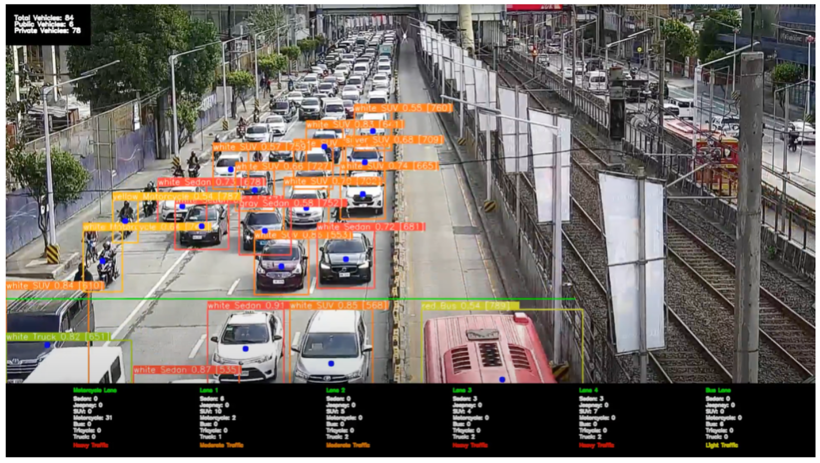
The processed results are recorded and, if requested, displayed. For each frame, the system can render bounding boxes around vehicles with labels indicating ID, vehicle type, and color (see Figure 8 for an example of an annotated output frame). It also maintains a log file (in text format) listing each detected vehicle, including frame ID, vehicle ID, class, color, bounding box coordinates, and detection confidence score. Additionally, summary statistics, including total counts per vehicle type, counts per lane, and current traffic conditions, are output for the video segment.

2.4. System Integration and Deployment

All components were integrated into a single Python program. We utilized the OpenCV library for video processing (reading frames and rendering output) and PyTorch for the YOLOv12 model. The program allows user-defined arguments, such as the input video path, whether to display the output live, and the output log file names. When executed, it processes the video sequentially, performing detection and tracking on each frame. A non-maximum suppression (NMS) step is applied to YOLO detections to eliminate duplicate overlapping boxes for the same object, using an IOU threshold of 0.45 (as default in YOLOv12).

Multiple vehicles in a single frame are each assigned distinct IDs by DeepSORT. These IDs persist until a vehicle leaves the frame, ensuring counting accuracy (a vehicle is counted only once when it crosses the counting line at the end of each lane). The system overlays the following on the video frames for visualization: bounding boxes (with different colors for each class), a label with Vehicle ID and class above each box, a colored dot or text indicating the identified color, and a textual banner at the top showing the current count per lane and traffic status. An example of an annotated frame is shown in Figure 8.

Finally, the system writes an output video file containing these annotations, along with a text report. The text report lists each vehicle’s ID, type, color, the frame number at first detection, and the total duration (in frames) it was tracked. This could be useful for post-processing or feeding into a database for traffic analysis.

3. Results

We evaluated the system using three 5 min CCTV video clips within the staged refinement workflow, labeled Video 1, Video 2, and Video 3, recorded from Metro Manila traffic surveillance scenes. These videos included a variety of scenarios, such as different times of day (morning, noon, afternoon) and varying traffic densities. Videos 1 and 2 were used primarily for fine-tuning, while Video 3 was used to evaluate the final performance after two rounds of fine-tuning. In addition to these three staged-evaluation clips, a separate fourth CCTV clip was reserved exclusively for the blind evaluation reported later in Section 3.2.

3.1. Vehicle Classification

For clarity, the study uses three different prediction levels. First, vehicle class refers to the binary public/private grouping used for higher-level traffic categorization. Second, vehicle type refers to the seven-category local taxonomy used in the detector, namely Sedan, SUV, Truck, Motorcycle, Jeepney, Tricycle, and Bus. Third, vehicle color is treated as a separate auxiliary attribute-recognition task. These levels are evaluated separately because they represent different levels of semantic difficulty and practical use.

The corresponding evaluation metrics are also reported separately. Public/private class, vehicle type, and vehicle color are evaluated using accuracy, precision, recall, and F1 score on manually reviewed video outputs, while detector-level model-development performance is summarized using precision–recall analysis and mean average precision on the synthetic validation split.

3.1.1. Initial Performance on Video 1

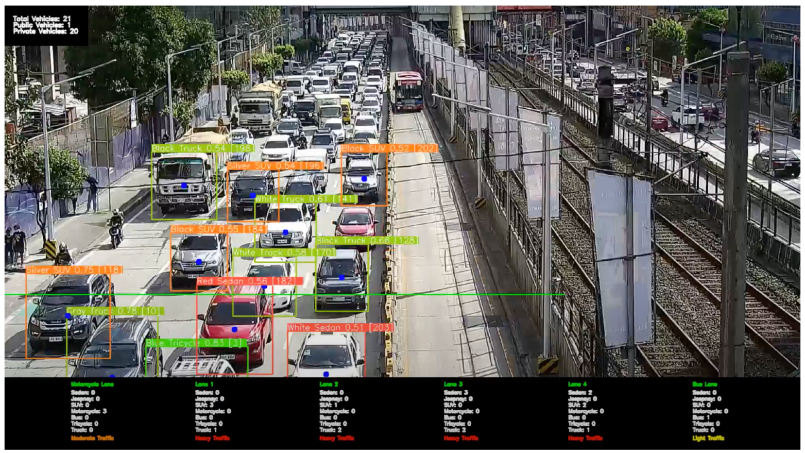
The model trained using a custom-generated dataset of 10,000 images produced the sample output frame illustrated in Figure 9. As observed in this figure, multiple vehicle detections occur as vehicles move closer to the camera. Consequently, the most critical data recorded were those vehicles that crossed the predefined counting line. Vehicles detected in the video were categorized according to their class and type.

Table 3. Performance Metrics for Video 1.

Vehicle Class
Class	Accuracy	Precision	Recall	F1 Score
Public	0.88	0.70	0.88	0.78
Private	0.99	1.00	0.99	0.99
Average	0.94	0.85	0.94	0.89
Vehicle Type
Type	Accuracy	Precision	Recall	F1 Score
Sedan	0.66	0.50	0.66	0.57
Jeepney	1.00	1.00	1.00	1.00
SUV	0.36	0.69	0.36	0.47
Motorcycle	1.00	0.98	1.00	0.99
Bus	0.88	0.78	0.88	0.82
Tricycle	1.00	1.00	1.00	1.00
Truck	0.92	0.42	0.92	0.58
Average	0.83	0.62	0.83	0.78
Vehicle Color
Color	Accuracy	Precision	Recall	F1 Score
White	0.88	0.94	0.88	0.91
Silver/Gray	0.92	0.61	0.92	0.73
Black	0.92	0.77	0.92	0.84
Red	0.81	1.00	0.81	0.90
Orange	0.60	1.00	0.60	0.75
Yellow	0.80	1.00	0.80	0.89
Green	1.00	1.00	1.00	1.00
Blue	0.73	1.00	0.73	0.84
Violet	1.00	1.00	1.00	1.00
Average	0.81	0.84	0.81	0.83

presents the corresponding performance metrics by vehicle class, type, and color for the first video sample. Vehicles were further grouped into public or private categories based on type: sedans, SUVs, motorcycles, and trucks were classified as private vehicles, while jeepneys, buses, and tricycles were categorized as public vehicles.

3.1.2. Fine-Tuning and Performance Improvement

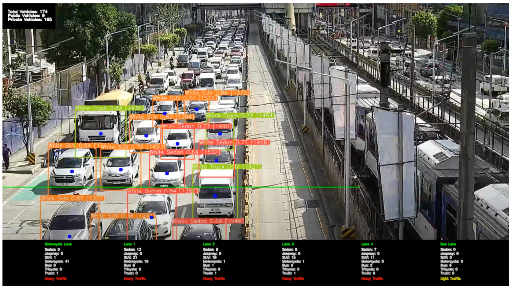
To improve performance, the system was fine-tuned using the output of the first video as an additional dataset. The text files were generated when the classified vehicle crossed the counting line and serve as the frame annotations. Before retraining, the annotations with incorrect classifications were manually corrected. Six frames per second were reviewed for errors, yielding 1800 frames for fine-tuning the second YOLOv12 model obtained from the generated custom dataset. This second YOLOv12 model was then further tested using the second five-minute video sample. Figure 10 shows the detection and classification results on the second test video, while

Table 4. Performance Metrics for Video 2.

Vehicle Class
Class	Accuracy	Precision	Recall	F1 Score
Public	1.00	0.85	1.00	0.92
Private	0.99	1.00	0.99	1.00
Average	1.00	0.93	1.00	0.96
Vehicle Type
Type	Accuracy	Precision	Recall	F1 Score
Sedan	0.81	0.91	0.81	0.86
Jeepney	1.00	1.00	1.00	1.00
SUV	0.93	0.80	0.93	0.86
Motorcycle	1.00	1.00	1.00	1.00
Bus	1.00	0.85	1.00	0.92
Tricycle	1.00	1.00	1.00	1.00
Truck	0.57	0.94	0.57	0.71
Average	0.90	0.93	0.90	0.91
Vehicle Color
Color	Accuracy	Precision	Recall	F1 Score
White	0.91	0.95	0.91	0.93
Silver/Gray	0.75	1.00	0.75	0.86
Black	0.93	0.81	0.93	0.87
Red	0.71	1.00	0.71	0.83
Orange	0.80	1.00	0.80	0.89
Yellow	0.85	1.00	0.85	0.92
Green	1.00	1.00	1.00	1.00
Blue	0.67	1.00	0.67	0.80
Violet	1.00	1.00	1.00	1.00
Average	0.82	0.93	0.82	0.86

presents the corresponding performance metrics.

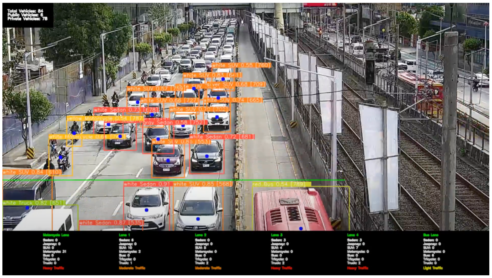
The system was then fine-tuned again using the output of the second video as an additional dataset. This stage again produced 1800 frames for fine-tuning. The resulting third YOLOv12 model was then evaluated on the third video sample. Figure 11 shows the detection and classification outputs for the third test video, and

Table 5. Performance Metrics for Video 3.

Vehicle Class
Class	Accuracy	Precision	Recall	F1 Score
Public	0.94	1.00	0.94	0.97
Private	1.00	1.00	1.00	1.00
Average	0.97	1.00	0.97	0.99
Vehicle Type
Type	Accuracy	Precision	Recall	F1 Score
Sedan	0.98	0.90	0.98	0.94
Jeepney	1.00	1.00	1.00	1.00
SUV	0.91	0.82	0.91	0.87
Motorcycle	1.00	1.00	1.00	1.00
Bus	0.94	1.00	0.94	0.97
Tricycle	1.00	1.00	1.00	1.00
Truck	0.48	0.88	0.48	0.62
Average	0.90	0.94	0.90	0.91
Vehicle Color
Color	Accuracy	Precision	Recall	F1 Score
White	0.95	0.98	0.95	0.97
Silver/Gray	0.89	0.53	0.89	0.67
Black	0.94	0.87	0.94	0.91
Red	0.80	1.00	0.80	0.89
Orange	0.75	0.60	0.75	0.67
Yellow	0.89	0.89	0.89	0.89
Green	1.00	1.00	1.00	1.00
Blue	0.73	1.00	0.73	0.84
Violet	0.50	1.00	0.50	0.67
Average	0.82	0.87	0.82	0.82

presents the corresponding performance metrics.

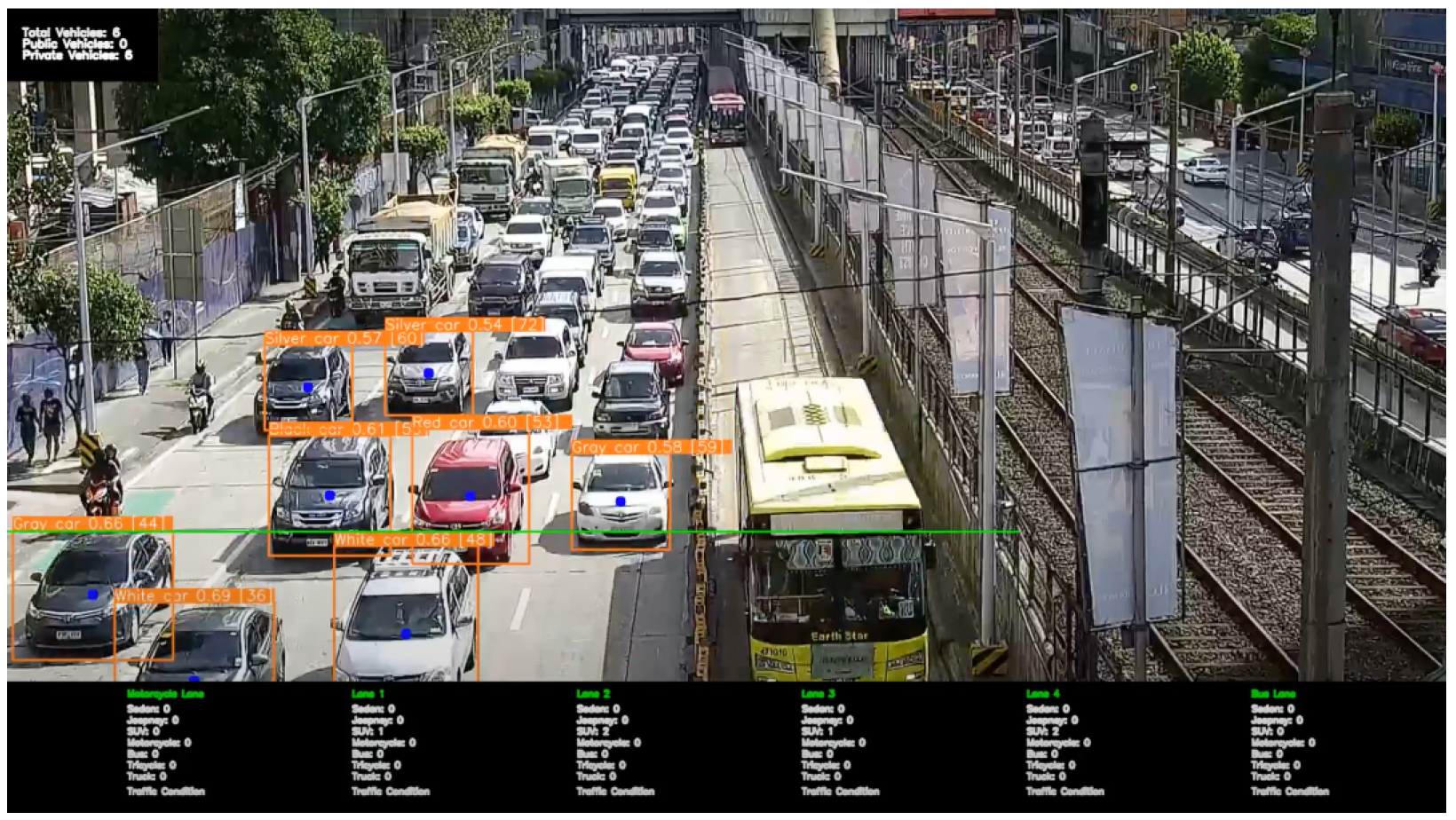
The baseline YOLOv12 model, using its original pretrained weights, was also applied for vehicle detection and classification in Video 3. This experiment aimed to evaluate and contrast the performance of the baseline model with the proposed fine-tuned version. The original model was pretrained on the COCO dataset and supported a limited set of vehicle categories, namely sedans, motorcycles, trucks, and buses. The detection and classification outputs produced by the baseline YOLOv12 are illustrated in Figure 12, while the corresponding performance metrics for vehicle class and type are summarized in

Table 6. Performance Metrics of Video 3 using Backbone YOLOv12 model.

Vehicle Class
Class	Accuracy	Precision	Recall	F1 Score
Public	0.89	1.00	0.89	0.94
Private	0.95	0.99	1.00	0.99
Average	0.95	1.00	0.95	0.97
Vehicle Type
Type	Accuracy	Precision	Recall	F1 Score
Sedan	0.99	0.93	0.99	0.96
Jeepney	N/A	N/A	N/A	N/A
SUV	N/A	N/A	N/A	N/A
Motorcycle	1.00	1.00	1.00	1.00
Bus	0.89	1.00	0.89	0.94
Tricycle	N/A	N/A	N/A	N/A
Truck	0.24	0.67	0.24	0.35
Average	0.78	0.90	0.78	0.81

.

Vehicle classification results from the pretrained model 1 and the fine-tuned model 3, compared to the YOLOv12 backbone model, were comparable, since private and public vehicle classification cover four and three types of vehicles, respectively. Major discrepancies can be seen on vehicle type prediction. The accuracy for each vehicle type cannot be directly compared because the backbone model predicts both sedans and SUVs as sedans, whereas the pretrained and fine-tuned models (3) classify them separately. It is worth noting that significant improvements in accuracy can be seen on sedans, SUVs, and buses from the pretrained model 1 to the fine-tuned model 3, yielding desirable outputs. It can also be observed that both the fine-tuned model 3 and the backbone model performed poorly at detecting trucks in the scene. In this case, both models can be further trained by increasing the presence of trucks in the dataset.

A significant finding in this testing is the improvement in vehicle classification accuracy from the pretrained model to the iterative fine-tuning process proposed in this research.

Table 7. Comparison of Average Accuracy Percentage for Videos 1, 2, and 3.

Average Accuracy
Features	Video 1	Video 2	Video 3
Class	94%	100%	97%
Type	83%	90%	90%
Color	81%	82%	82%
Count	92.67%	93.00%	96.67%

summarizes the accuracy for each feature across all three video samples.

3.2. Blind Evaluation Without On-the-Fly Retraining

Because the staged refinement workflow uses development videos for supervised correction and additional fine-tuning, a separate blind evaluation summary is included to distinguish development-stage adaptation from final frozen-model testing. This blind evaluation used a separate fourth CCTV clip that was not part of Videos 1–3 and was not used for retraining, annotation correction, threshold adjustment, or model selection. Two evaluation conditions were considered: a zero-shot real-world condition, in which the model trained only on synthetic data was applied directly to the blind CCTV video, and an adapted blind condition, in which the model refined using Videos 1 and 2 only was evaluated on the same blind CCTV video with no further updates.

Table 8. Comparison of zero-shot blind real-world performance, adapted blind real-world performance, and the previously reported staged post-refinement result. The blind test video was not used for training, threshold adjustment, or further refinement.

Metric	Zero-Shot Blind Real-World	Adapted Blind Real-World	Existing Staged Post-Refinement
Public/Private Class Accuracy	92.43%	95.16%	97.00%
Vehicle-Type Accuracy	86.17%	88.62%	90.00%
Color Accuracy	74.50%	79.87%	82.00%
Count Accuracy	91.22%	94.00%	96.67%

is intended to present these blind-study results alongside the previously reported staged post-refinement performance. In general, the zero-shot blind result is expected to reflect the synthetic-to-real transfer capability of the initial detector, whereas the adapted blind result reflects the benefit of controlled refinement prior to deployment. The staged post-refinement result is retained for comparison, but should be interpreted separately because it belongs to the development-oriented adaptation workflow described earlier.

The blind-study results followed the expected trend: the zero-shot blind evaluation was lower than the adapted blind evaluation, while the adapted blind performance remained slightly below the previously reported staged post-refinement result. This behavior is consistent with the role of staged refinement in improving deployment readiness without implying on-the-fly retraining during final testing.

4. Discussion

4.1. Robustness

The term “robust” in this study refers to the system’s ability to maintain useful performance after synthetic pretraining followed by limited real-world refinement under the tested CCTV conditions. While the results indicate promising transferability within similar traffic-monitoring scenarios, the current evaluation scale does not yet support a strong claim of universal generalization across arbitrary cities, viewpoints, lighting conditions, or camera geometries. The initial synthetic training and staged fine-tuning strategy nevertheless enabled the model to learn a useful representation of the target vehicle categories under the tested surveillance setup. At the same time, substantial shifts in scene characteristics—such as nighttime imagery, severe glare, or markedly different camera viewpoints—would still be expected to require additional adaptation data.

4.2. Speed

The runtime performance of the integrated YOLOv12 + DeepSORT pipeline was evaluated under the hardware setup used in this study. At a video resolution of 1280 × 720, the system processed approximately 20 frames per second on an NVIDIA RTX 2070 GPU, which is sufficient for near-real-time operation in practical monitoring scenarios. Under CPU-only execution, the processing rate decreased to approximately 1 frame per second, making CPU-only use more suitable for offline analysis. These results indicate that GPU acceleration is important for deployment. The present runtime assessment was limited to the tested resolution and hardware platform; benchmarking across multiple input resolutions and deployment devices remains future work.

4.3. Comparison with Baseline Models

Compared to the baseline pretrained YOLOv12 (trained on the COCO dataset with classes such as “car”, “motorbike”, etc.), our fine-tuned model significantly outperforms it in our domain. The baseline YOLOv12 (COCO) treated all cars, SUVs, and pickup trucks as “car” and did not distinguish subtypes, and it missed many motorcycles or misclassified them because of differences in context (COCO training might not include dense traffic scenes from a fixed CCTV perspective). We quantified the baseline’s performance on Video 3: it detected only 195 out of 300 vehicles (65% recall) and produced some false positives. In contrast, after training, our model detected 278 out of 300 (93% recall) in the same video and provided detailed classification.

When compared with prior work, ref. [1] reported 86.7% accuracy in their vehicle classification system, which is slightly lower than our 90% for vehicle type and 97% for class. Ref. [16] achieved 96.1% accuracy in color recognition, higher than our 82%, likely because their setup was more controlled (a highway camera with a consistent view and a specialized color-extraction CNN). Our integrated approach sacrifices some color accuracy for generality. The study in [17] achieved 96.8% accuracy in classifying traffic situations (light/medium/heavy) using symbolic data analysis. Our traffic-state module is intended as a practical rule-based estimation component driven by vehicle-count trends rather than as a separately trained supervised classifier. Accordingly, although it produced operationally useful light/moderate/heavy labels during testing, we did not perform a formal quantitative benchmark against independently labeled traffic-state ground truth in the present study. This remains an important direction for future work.

The lower performance observed for vehicle type and color recognition relative to counting and public/private class prediction reflects the greater difficulty of these attribute-recognition tasks under CCTV conditions. In particular, visually similar categories such as sedan and SUV, as well as reflective color pairs such as white and gray/silver, remain more sensitive to viewpoint, scale, and illumination effects. For this reason, the revised manuscript reports the metrics for these attributes separately and discusses them explicitly rather than relying only on aggregate accuracy.

From a methodological perspective, the present study differs from prior traffic-monitoring works not merely by combining detection and tracking, but by coupling a scene-aware semi-automated synthetic-data workflow with staged real-world refinement and downstream operational modules in a single deployable system. The contribution is therefore best understood as an integrated CCTV-monitoring framework for practical adaptation under limited real-world annotation resources, rather than as a claim of novelty in object detection or tracking alone.

The comparative scope of the present study includes two levels. First, a preliminary detector-selection comparison was performed among YOLOv12, Faster R-CNN, and SSD MobileNetv2 FPNlite under the same initial conditions, which motivated the selection of YOLOv12 for the final pipeline. Second, the final refined detector was compared against the baseline backbone YOLOv12 model during CCTV-based evaluation. These comparisons establish the practical benefits of the refined detector within the scope of the present study. However, broader end-to-end comparisons against additional modern traffic-monitoring pipelines, such as YOLOv8 + DeepSORT or alternative tracking frameworks, were not performed and remain an important direction for future work.

4.4. Limitations

Some limitations have been noted: (1) Color detection is less reliable under certain conditions (e.g., glare, low light, similar colors). (2) The system currently does not handle nighttime videos—a separate set of training (including thermal or infrared imagery if available) would be needed for robust nocturnal operation. (3) Our vehicle classes did not include some special cases like pickup trucks or public utility vans (treated as SUVs). Depending on the use case, the classification taxonomy might be expanded. (4) The reliance on a static camera—if the camera moves or shakes, tracking might break. In our tests, the cameras were fixed in place. (5) As with any learned system, extreme scenarios (accidents, unusual vehicle types) were not in the training data and may not be handled correctly.

An additional limitation is the modest scale of the real-world evaluation. The present study used three 5 min CCTV videos within the staged refinement workflow, with Videos 1 and 2 serving as development videos for iterative refinement and Video 3 serving as the final post-refinement evaluation video. In addition, a separate fourth CCTV clip was reserved for blind frozen-model evaluation. Although this protocol strengthens the separation between development and testing, the overall real-world evaluation scale remains modest and does not yet constitute a broad benchmark of generalization across multiple unseen sites, camera viewpoints, lighting conditions, or traffic environments. The results demonstrate that synthetic pretraining combined with limited real-world refinement can improve CCTV-based vehicle monitoring while reducing the amount of manually labeled real-world data required. However, because the current real-world evaluation remains limited in scale, the findings should be interpreted as evidence of feasibility and location-adaptable deployment rather than conclusive proof of universal performance across arbitrary intersections or cities.

Another limitation is that the traffic-state component was evaluated operationally rather than through a formal supervised classification benchmark. Because no independently labeled traffic-condition ground truth was available for the tested videos, quantitative performance indicators for light/moderate/heavy traffic-state assignment were not computed in the present study. Future work should construct a labeled traffic-state dataset so that this module can be evaluated using standard classification metrics.

A further limitation is that tracking was assessed indirectly through counting consistency and qualitative ID persistence rather than standardized multi-object tracking metrics such as MOTA, MOTP, or ID switches. This is because frame-level identity annotations were not available for the CCTV videos used in the present study. Future work should therefore construct or adopt an annotated traffic-tracking benchmark so that the tracking component can be evaluated using standard MOT metrics.

5. Conclusions

We have presented a robust CCTV-based vehicle monitoring system that integrates object detection, multi-object tracking, counting, vehicle categorization, color attribution, and traffic-state estimation using YOLOv12 and DeepSORT. The study combined a semi-automated synthetic-data generation workflow with staged real-world refinement to reduce manual annotation effort while improving deployment readiness under the tested CCTV conditions.

The detector achieved an overall $mAP@0.5$ of 0.977 on the synthetic validation split, indicating strong in-domain learning during the initial training stage. In the real-world CCTV evaluation, the refined system achieved average accuracies of 97% for public/private vehicle class prediction, 90% for vehicle-type prediction, 82% for vehicle-color recognition, and 96.67% for vehicle counting on the final post-refinement evaluation video. These results show that synthetic pretraining combined with limited real-world refinement can improve CCTV-based vehicle monitoring while reducing the amount of manually labeled real-world data required.

The findings support the feasibility of using an integrated YOLOv12–DeepSORT pipeline for practical traffic-monitoring applications under the tested conditions. In particular, the staged refinement strategy helped reduce the synthetic-to-real performance gap and improved the system’s ability to operate on actual surveillance footage. At the same time, the study should be interpreted as a proof-of-feasibility for location-adaptable deployment rather than conclusive evidence of universal generalization across arbitrary cities, viewpoints, lighting conditions, or camera geometries.

Several limitations remain. The real-world evaluation included three 5 min CCTV videos within the staged refinement workflow, together with a separate fourth blind CCTV clip reserved for frozen-model testing. Although this protocol improves the separation between development and final evaluation, it is still insufficient to establish broad no-retraining generalization across diverse sites, viewpoints, and lighting conditions. Vehicle-color recognition remained less reliable than counting and public/private categorization, especially under reflective or visually ambiguous conditions. In addition, the traffic-state module was implemented as a rule-based estimation component rather than a separately benchmarked supervised classifier, and the tracking component was not evaluated using standardized multi-object tracking metrics such as MOTA, MOTP, or ID switches because frame-level identity annotations were not available.

Future work should therefore focus on broader evaluation across multiple unseen intersections, cities, camera viewpoints, and lighting conditions without additional retraining. Further improvements may include developing a more advanced color-recognition module, constructing labeled datasets for traffic-state and tracking benchmarks, incorporating incident detection capabilities, and optimizing the system for deployment on edge devices or CPU-only platforms.

References

1. Ambata, L.U.; del Castillo, I.A.P.; Jacinto, J.R.H.; Santos, C.M.T. Public and Private Vehicle Quantification and Classification using Vehicle Detection and Recognition. In Proceedings of the 2019 IEEE 11th International Conference on Humanoid, Nanotechnology, Information Technology, Communication and Control, Environment, and Management (HNICEM); IEEE: New York, NY, USA, 2019; pp. 1–6. [Google Scholar] [CrossRef]
2. Tilakaratna, D.S.B.; Watchareeruetai, U.; Siddhichai, S.; Natcharapinchai, N. Image analysis algorithms for vehicle color recognition. In Proceedings of the 2017 International Electrical Engineering Congress (iEECON); IEEE: New York, NY, USA, 2017; pp. 1–4. [Google Scholar] [CrossRef]
3. Tang, Y.; Zhang, C.; Gu, R.; Li, P.; Yang, B. Vehicle detection and recognition for intelligent traffic surveillance system. Multimed. Tools Appl. 2017, 76, 5817–5832. [Google Scholar] [CrossRef]
4. Ambata, L.U.; Dalangin, R.E.A.; Duaqui, I.A.M.; Saavedra, J.V.V.; Veloria, M.J.V.; Abayan, J.J.A.; Bandala, A.A.; Agulto, R.P. A Jetson TX2-Based License Plate Recognition and GPS Tracking System for Vehicular Surveillance. In Proceedings of the 2025 IEEE International Conference on Future Machine Learning and Data Science (FMLDS); IEEE: New York, NY, USA, 2025; pp. 219–224. [Google Scholar] [CrossRef]
5. Madhumitha, M.; Dhivya, P. Vehicle Recognition and Compilation in Database Software. In Proceedings of the 2020 International Conference on System, Computation, Automation and Networking (ICSCAN); IEEE: New York, NY, USA, 2020; pp. 1–5. [Google Scholar] [CrossRef]
6. Zhou, C.; Fan, T. A Vehicle Recognition Method Based on Multi-Camera Information. In Proceedings of the 2019 Chinese Control Conference (CCC); IEEE: New York, NY, USA, 2019; pp. 7835–7839. [Google Scholar] [CrossRef]
7. Shvai, N.; Hasnat, A.; Meicler, A.; Nakib, A. Accurate Classification for Automatic Vehicle-Type Recognition Based on Ensemble Classifiers. IEEE Trans. Intell. Transp. Syst. 2020, 21, 1288–1297. [Google Scholar] [CrossRef]
8. Ma, Z.; Chang, D.; Xie, J.; Ding, Y.; Wen, S.; Li, X.; Si, Z.; Guo, J. Fine-Grained Vehicle Classification With Channel Max Pooling Modified CNNs. IEEE Trans. Veh. Technol. 2019, 68, 3224–3233. [Google Scholar] [CrossRef]
9. Rothmeier, T.; Huber, W.; Knoll, A.C. Time to Shine: Fine-Tuning Object Detection Models with Synthetic Adverse Weather Images. In Proceedings of the IEEE/CVF Winter Conference on Applications of Computer Vision (WACV); IEEE: New York, NY, USA, 2024. [Google Scholar]
10. Staniszewski, M.; Kempski, A.; Marczyk, M.; Socha, M.; Foszner, P.; Cebula, M.; Labus, A.; Cogiel, M.; Golba, D. Searching for the Ideal Recipe for Preparing Synthetic Data in the Multi-Object Detection Problem. Appl. Sci. 2025, 15, 354. [Google Scholar] [CrossRef]
11. Fei, L.; Han, B. Multi-Object Multi-Camera Tracking Based on Deep Learning for Intelligent Transportation: A Review. Sensors 2023, 23, 3852. [Google Scholar] [CrossRef] [PubMed]
12. Kumar, S.; Singh, S.K.; Varshney, S.; Singh, S.; Kumar, P.; Kim, B.G.; Ra, I.H. Fusion of Deep Sort and Yolov5 for Effective Vehicle Detection and Tracking Scheme in Real-Time Traffic Management Sustainable System. Sustainability 2023, 15, 16869. [Google Scholar] [CrossRef]
13. Bui, T.; Wang, G.; Wei, G.; Zeng, Q. Vehicle Multi-Object Detection and Tracking Algorithm Based on Improved You Only Look Once 5s Version and DeepSORT. Appl. Sci. 2024, 14, 2690. [Google Scholar] [CrossRef]
14. Ji, A.; Ma, X. Vehicle Detection and Classification for Traffic Management and Autonomous Systems Using YOLOv10. Alex. Eng. J. 2025, 127, 804–816. [Google Scholar] [CrossRef]
15. Mohd Ali, N.; Md Rashid, N.K.A.; Mustafah, Y.M. Performance Comparison between RGB and HSV Color Segmentations for Road Signs Detection. Appl. Mech. Mater. 2013, 393, 550–555. [Google Scholar] [CrossRef]
16. Kim, K.J.; Kim, P.K.; Lim, K.T.; Chung, Y.S.; Song, Y.J.; Lee, S.I.; Choi, D.H. Vehicle Color Recognition via Representative Color Region Extraction and Convolutional Neural Network. In Proceedings of the 2018 Tenth International Conference on Ubiquitous and Future Networks (ICUFN); IEEE: New York, NY, USA, 2018; pp. 89–94. [Google Scholar] [CrossRef]
17. Dallalzadeh, E.; Guru, D.S. Content-based classification of traffic videos using symbolic features. In Proceedings of the 2014 International Conference on Advances in Computing, Communications and Informatics (ICACCI); IEEE: New York, NY, USA, 2014; pp. 288–294. [Google Scholar] [CrossRef]
Figure 1. System Architecture Overview.
Smartcities 09 00085 g001
Figure 2. Semi-Automated Dataset Creation Process.
Smartcities 09 00085 g002
Figure 3. Flowchart of Dataset Creation.
Smartcities 09 00085 g003
Figure 4. Sample Output Image of Dataset Creation.
Smartcities 09 00085 g004
Figure 5. Normalized confusion matrix on the synthetic validation split after the initial training stage. This figure reflects in-domain validation performance on the generated dataset and should not be interpreted as the final real-world CCTV evaluation.
Smartcities 09 00085 g005
Figure 6. (a) Precision–Confidence Curve; (b) Recall–Confidence Curve; (c) Precision–Recall Curve; (d) F1–Confidence Curve.
Smartcities 09 00085 g006
Figure 7. Training and Fine-Tuning Workflow.
Smartcities 09 00085 g007
Figure 8. Example Output Frame with Annotations.
Smartcities 09 00085 g008
Figure 9. Frame from Video 1 using Model 1 from Synthetic Dataset.
Smartcities 09 00085 g009
Figure 10. Frame from Video 2 using Model 2.
Smartcities 09 00085 g010
Figure 11. Frame from Video 3 using Model 3.
Smartcities 09 00085 g011
Figure 12. Frame from Video 3 using Backbone YOLOv12 Model.
Smartcities 09 00085 g012