A Timed Petri Net-Based Dynamic Visitor Guidance Model for Mountain Scenic Areas During Peak Periods

Highlights

What are the main findings?

• Peak-period congestion in large scenic areas is a system-level phenomenon driven by positive feedback loops of hotspot accumulation and load propagation rather than an unavoidable consequence of high visitor volume.
• Simulation experiments indicate that Timed Petri Net–based guidance strategies can substantially improve load distribution and alleviate congestion imbalance under simulated peak-period scenarios.

What are the implications of the main findings?

• Scenic area management should shift from entrance-side volume control to continuous internal flow regulation, maintaining operations within an optimal load range that balances safety and visitor experience.
• The proposed guidance framework enables robust, real-time implementation using only local information, offering a practical decision-support tool for smart tourism and smart city management systems.

Abstract

Tourist congestion and load imbalance during peak periods pose critical challenges to the safe operation and experience assurance of large scenic areas. To address the limitations of traditional management approaches in capturing the dynamic and stochastic nature of tourist flows, this study develops a dynamic visitor guidance modeling and analysis framework based on a Timed Petri Net. The proposed model provides a formal representation of tourist movements, scenic spot load evolution, and guidance decision mechanisms within a scenic area. Under unified parameter settings and controlled random conditions, multiple visitor guidance strategies with different information coverage scopes are designed, and minute-level simulation experiments are conducted using the Huangshan Scenic Area as a case study. The simulation results show that, compared with unguided tourist flows, the proposed strategies significantly reduce average load levels, alleviate spatial load imbalance, and enhance TS. Using mean–standard deviation analysis, distributional analysis, and dynamic evolution analysis, differences among guidance strategies in terms of load control, visitor experience, and operational stability are systematically evaluated. Furthermore, a quantitative relationship model between tourist satisfaction and scenic area load is constructed, revealing a consistent inverted-U pattern. Robustness tests under multiple random seeds indicate that the main conclusions are not sensitive to specific stochastic realizations. Overall, the simulation results suggest that dynamic visitor guidance may improve load control, visitor experience, and system stability by optimizing the spatiotemporal distribution of tourist flows, thereby providing simulation-based quantitative insights for peak-period management in large scenic areas.

1. Introduction

With the normalization of mass tourism, concentrated visitor flows and localized congestion during peak periods have become common governance challenges for popular destinations worldwide [1]. In China, domestic tourism reached 6.006 billion trips in 2019 and rebounded to 5.62 billion trips in 2024 after the COVID-19 disruption [2,3]. Such large-scale tourism demand often leads to instantaneous overload and localized congestion in popular scenic areas, which may undermine visitor experience and even introduce ecological and safety risks [1,4]. Therefore, achieving effective visitor flow guidance and load balancing during peak periods has become an important issue for the refined management and intelligent operation of scenic areas.

In response to these challenges, many destinations have adopted management measures such as visitor quotas, reservation systems, and time-shifted visitation to regulate entrance flows [5,6,7,8]. Meanwhile, smart tourism research has increasingly emphasized data-driven monitoring, early warning, and decision support for complex operational environments [9,10,11,12]. However, existing studies suggest that, without explicit capacity constraints and interpretable decision logic, these approaches remain insufficient for managing highly dynamic peak-period congestion within scenic-area networks [13].

Existing studies have examined peak-period visitor management from multiple perspectives [14,15,16,17,18,19,20,21,22,23,24,25,26,27,28], yet several limitations remain. Existing approaches often emphasize entry-stage regulation, while internal congestion and spatial load imbalance may still emerge in large scenic areas even under controlled entrance flows [18,19]. In addition, congestion is often treated implicitly rather than as an explicit capacity constraint, and robustness under stochastic visitor arrivals is still insufficiently examined in many existing models [20,21,22,23,24,25,26,27,28].

Timed Petri Nets provide a suitable modeling framework for this problem because they can explicitly represent concurrency, capacity constraints, temporal dependencies, and state transitions in complex visitor flow systems [29,30]. However, their application to peak-period visitor guidance in large scenic areas remains limited, especially for multi-path and bidirectional flow settings [31,32].

To address these gaps, this study proposes a TPN-based dynamic visitor guidance model for peak tourism periods. Attractions are abstracted as resource units with explicit capacity and time constraints, while visitor movements between attractions are modeled as state transitions, enabling a unified formal representation of bidirectional and parallel tourist flows. Based on operational requirements during peak periods, four categories of guidance strategies are designed according to different information coverage scopes, including Equal allocation, attraction-weight-based guidance, scenic spot load-based guidance, and route load-based guidance. Using the Huangshan Scenic Area as a case study, minute-level simulation experiments are conducted to evaluate the performance and stability of different strategies under stochastic arrival conditions.

The main contributions of this study are threefold. First, it introduces a TPN-based framework for modeling dynamic visitor guidance during peak periods in large scenic areas. Second, it develops four guidance strategies under different information conditions to evaluate alternative redistribution mechanisms. Third, it establishes a simulation-based evaluation framework to compare strategy performance in terms of congestion control, spatial balance, visitor satisfaction, and robustness.

It should be noted that this study aims to develop a modeling and decision-support framework for analyzing congestion propagation and evaluating visitor guidance strategies under controlled peak-period scenarios, rather than proposing a fully operational real-time control system.

2. Related Work

2.1. Visitor Crowding Perception and Carrying Capacity

Research on visitor congestion has shown that perceived crowding and visitor satisfaction are influenced not only by visitor numbers, but also by expectations, spatial conditions, and management objectives [14,15]. Studies further distinguish between physical and social crowding, both of which negatively affect visitor experience and destination attractiveness [16], while social carrying capacity research emphasizes that once visitor intensity exceeds socio-psychological thresholds, satisfaction declines markedly and avoidance behaviors increase [4]. Related work in environmental psychology also shows that crowding perception and satisfaction are shaped by social stimuli and environmental conditions [17].

2.2. Demand-Side Regulation and Entry Control Strategies

Another major stream of research focuses on demand-side regulation, particularly through institutional tools such as visitor quotas, reservation systems, and time-slot management. Studies on time-based entry control in national parks and popular attractions show that reservation systems can effectively alleviate entrance congestion, improve visitor experience, and enhance public acceptance of management measures [18,19].

Building on this foundation, researchers have introduced forecasting models and big-data-driven approaches to support visitor flow prediction and early warning. Time-series methods such as ARIMA and its variants have been widely applied to forecast tourism demand and peak-period flows [20], while machine learning and hybrid models have further improved prediction accuracy and responsiveness [21]. These approaches provide valuable prior information for management decision-making. However, reservation- and prediction-oriented tools mainly operate at the entry stage. For large scenic areas with complex internal structures, internal congestion and spatial load imbalance may still emerge even when entrance flows are well regulated, limiting the effectiveness of entry-side control alone.

2.3. Simulation and Optimization for Internal Visitor Guidance

To address internal congestion, a growing number of studies have adopted simulation and optimization methods to model visitor movement and evaluate guidance strategies within scenic areas. Multi-agent simulation, discrete-event simulation, and heuristic optimization algorithms have been widely used to represent visitor route choice, dwelling behavior, and dynamic interactions with congestion states [22,23,24,25,26,27,28]. These studies demonstrate that simulation-based approaches are effective in capturing visitor heterogeneity, complex spatial interactions, and multi-objective trade-offs.

At the route optimization level, genetic algorithms, ant colony algorithms, and their variants have been employed to search for optimal touring paths under time, cost, and congestion constraints [26,27,28]. These methods enhance operational efficiency and improve visitor experience by adjusting routes dynamically. Nevertheless, in many models, congestion is treated as a penalty term within utility functions rather than being explicitly represented as hard capacity constraints. Moreover, model semantics are often tightly coupled to specific algorithms or simulation platforms, reducing interpretability and limiting cross-scenario transferability of guidance strategies.

While agent-based models (ABMs) are useful for representing heterogeneous visitor behavior, the present study focuses on system-level congestion propagation and rule-based visitor guidance within a scenic-area network.

2.4. TPN-Based Modeling for Resource-Constrained Systems

TPNs are a formal modeling tool with rigorous mathematical semantics and have been widely applied in resource-constrained and concurrent systems such as transportation, manufacturing, and logistics [29]. Their strengths lie in the natural representation of concurrency, conflicts, resource sharing, and system reachability within a unified framework. By incorporating temporal extensions, TPNs can further capture system evolution under time constraints, making them suitable for modeling dynamic processes characterized by parallel operations and limited resources [30].

In tourism-related applications, the use of Petri nets remains relatively limited. Existing studies have primarily focused on simplified scenic structures, such as unidirectional routes or single-entry–single-exit systems, and often examine only a single guidance or classification dimension [31,32]. Systematic comparison of multiple guidance strategies under unified models, as well as robustness testing under stochastic visitor arrivals, has received little attention. These limitations suggest the need for a more comprehensive TPN-based modeling approach capable of representing multi-entry, multi-path, and bidirectional visitor flows, while supporting interpretable and robust guidance decision-making.

Although the related work is organized into four subsections, several distinct methodological streams can be identified across the reviewed studies. To provide a clearer overview of these research directions, representative studies are summarized in

Table 1. Summary of representative studies on tourist flow modeling and visitor guidance.

Reference	Authors	Year	Research Problem	Solution Method
[4,14,15,16,17]	Saveriades; Manning; Shelby & Heberlein; Yin et al.; Ruiz et al.	1986–2021	Understanding the relationship between perceived crowding, visitor experience, and social carrying capacity	Survey-based studies and environmental psychology approaches
[18,19]	Creany et al.; Miller et al.	2023–2024	Managing visitor inflow and alleviating entrance congestion in popular attractions	Reservation systems and time-slot entry management
[20,21,24]	Li et al.; Xu et al.; Zhang et al.	2020–2024	Predicting tourist arrivals and peak-period demand	Time-series forecasting and machine learning approaches
[22,23,25]	Chang et al.; Tang et al.; Cheng et al.	2023–2025	Modeling visitor movement, route choice, and congestion interactions within scenic areas	Multi-agent simulation and simulation-based modeling approaches
[26,27,28]	Qi & Wang; Li et al.; Liang et al.	2021–2022	Searching for optimal tourism routes under time, cost, and congestion constraints	Genetic algorithms and ant colony optimization
[29,30,31,32]	Murata; Zuberek; Su & Li; Lu et al.	1989–2022	Modeling resource-constrained dynamic systems and tourist diversion processes	Timed Petri Net modeling

.

Compared with behavior-oriented simulation approaches, the TPN framework emphasizes the structural and temporal characteristics of visitor flow systems and is particularly suitable for analyzing congestion propagation and rule-based visitor guidance under capacity constraints. Existing Petri-net-based applications in tourism remain limited, especially in terms of systematic comparison of alternative guidance strategies under unified modeling frameworks. Motivated by these gaps, this study develops a TPN-based dynamic visitor guidance model for peak-period management in large scenic areas.

3. Methodology

3.1. A TPN–Based Dynamic Visitor Guidance Model

To capture the dynamic and stochastic characteristics of visitor movements within scenic areas, this study adopts a TPN as the core modeling approach. A TPN $\mathrm{\Sigma }=\left(P,T,F,\omega ,\delta ,\phi ,f,m_0,M\right)$ is constructed to describe the dynamic visitor guidance process in scenic areas.

Let $P=\left\{p_1,p_2,\cdots ,p_n\right\}$ denote a finite set of places, corresponding to scenic attractions, with n representing the number of attractions; let $T=\left\{t_1,t_2,\cdots ,t_m\right\}$ denote a finite set of transitions, representing visitor flow movements between attractions, with m indicating the number of flow transitions; let $F=\left(P\times T\right)\cup \left(T\times P\right)$ denote a finite set of directed arcs connecting places and transitions. For each transition, $P\to T$ maps a transition to the multiset of its output places, representing the visitor flows diverted from an attraction, while $T\to P$ maps a transition to the multiset of its input places, representing the visitor flows entering an attraction. Let $\omega =\left({\omega }_1^n,{\omega }_2^n,\cdots ,{\omega }_m^n\right)$ denote the weight function associated with each directed arc, and let m be the total number of directed arcs. For a pair of attractions, the number of directed arcs between them is denoted n accordingly and ${\displaystyle \sum {\omega }_i^n}=1$; in particular, when only a single directed arc exists between two attractions, its weight is set to 1. Let $\phi =\left({\phi }_1,{\phi }_2,\cdots ,{\phi }_n\right)$ represent the set of time constraints associated with places, corresponding to the average dwell time of visitors at each attraction. Let $\delta =\left({\delta }_1,{\delta }_2,\cdots ,{\delta }_n\right)$ denote the set of place weights, representing the overall attractiveness or popularity of attractions and visitors’ preference tendencies, with $\sum {\delta }_i=1$. Let $f={\left(f_{ij}\right)}_{n\times n}$ denote the time distance from attraction i to attraction i, expressed as the travel time required to move between the two attractions, where $f_{ij}=f_{ji},i,j=1,2,\cdots n$. Let $f_{ij}=f_{ji},i,j=1,2,\cdots n$ represent the initial marking of the system, indicating the initial number of visitors at each attraction. Let $m_0$ denote the initial number of visitors at each attraction, and $M$ denote the capacity constraint of each attraction, representing the maximum allowable number of visitors.

The main notations of the TPN model are presented in

Table 2. Main notations used in the TPN-based visitor guidance model.

Symbol	Meaning in the Timed Petri Net	Interpretation in the Scenic Area System
$P$	Finite set of places	Set of scenic spots in the scenic area
$T$	Finite set of transitions	Set of visitor flow transitions between scenic spots
$F$	Set of directed arcs connecting places and transitions	Set of connections (routes) between scenic spots
$\omega$	Weight associated with each arc	Proportion of visitors choosing a specific route between scenic spots
$\phi$	Time constraint associated with places	Average residence time of visitors at a scenic spot
$\delta$	Weight of places	Attractiveness weight of each scenic spot
$f$	Time delay of a transition	Travel time between scenic
$m_0$	Initial marking of places	Initial number of visitors at each scenic spot
$M$	Capacity constraint set of places	Capacity constraint set of scenic attractions
$M_i$	Capacity limit of place i	Maximum visitor capacity of scenic spot i
$p_{inout}$	Special place representing entrance/exit in forward direction	Entrance/exit node in the forward touring direction
$p_{outin}$	Special place representing entrance/exit in reverse direction	Entrance/exit node in the reverse touring direction
$p_i$	The i-th place in the Petri net	Scenic spot i in the scenic area network
$m_i$	Number of tokens in place $p_i$ (forward direction)	Current number of forward-direction visitors at scenic spot i
$m_i^{\prime }$	Number of tokens in place $p_i$ (reverse direction)	Current number of reverse-direction visitors at scenic spot i
$t_i$	Timed transition associated with place $p_i$	Transition representing visitor movement related to scenic spot i

, while the state variables used in the dynamic visitor guidance algorithm are summarized in

Table 3. The state variables used in the dynamic visitor guidance algorithm.

Symbol	Description
$H=\{h_1,h_2,\dots ,h_n\}$	Set of current numbers of tourists at each scenic spot
$J=\{j_1,j_2,\dots ,j_n\}$	Set of natural tourist distribution results under no management intervention
$A=\{a_1,a_2,\dots ,a_n\}$	Set of information on the number of tourists expected to enter the scenic area
$H^{\prime }=\{h_{1^{\prime }},h_{2^{\prime }},\dots ,h_{n^{\prime }}\}$	Set of operational states of scenic spots after natural distribution
$Q=\{q_1,q_2,\dots ,q_n\}$	Set of overload information for each scenic spot
$I=\{i_1,i_2,\dots ,i_n\}$	Set of guidance information generated under different tourist guidance strategies
$H^{″}=\{h_{1^{″}},h_{2^{″}},\dots ,h_{n^{″}}\}$	Final set of operational states of scenic spots after implementation of guidance strategies
$[t_1,t_2]$	Time interval under study
$\lambda (t)$	Time-dependent arrival intensity function in the NHPP model
${\widehat{\lambda }}_h$	Average arrival rate estimated for the $h-th$ time segment
$\Delta t$	Discrete simulation time step (one minute in this study)
$t_k=t_1+k\Delta t$	Discrete simulation time point
$X_k$	Number of newly arriving tourists at time step $t_k$
$l_{ij}$	Load rate of scenic spot i at time j
$e_{ij}$	Vacancy (idle) rate of scenic spot i at time j
$L_{ave}$	Weighted average load rate of the scenic area at time j
$E_{ij}$	Load-rate variance component of scenic spot i at time j

.

The proposed model further supports bidirectional visitor movements within scenic areas, allowing visitors to enter from different entrances, exit from different exits, and traverse attractions in opposite directions. At each discrete time step, the system updates the number of visitors at each attraction according to the dwell-time triggering mechanism and transition firing rules. When the number of visitors at an attraction exceeds its capacity threshold, the system activates the visitor guidance mechanism and dynamically redirects a portion of visitors to alternative attractions. By integrating capacity constraints, temporal evolution, and bidirectional flow characteristics within a unified formal representation, the TPN provides a flexible and interpretable modeling tool for representing peak-period operations in scenic areas. This framework also establishes a solid foundation for the subsequent design and analysis of visitor guidance strategies.

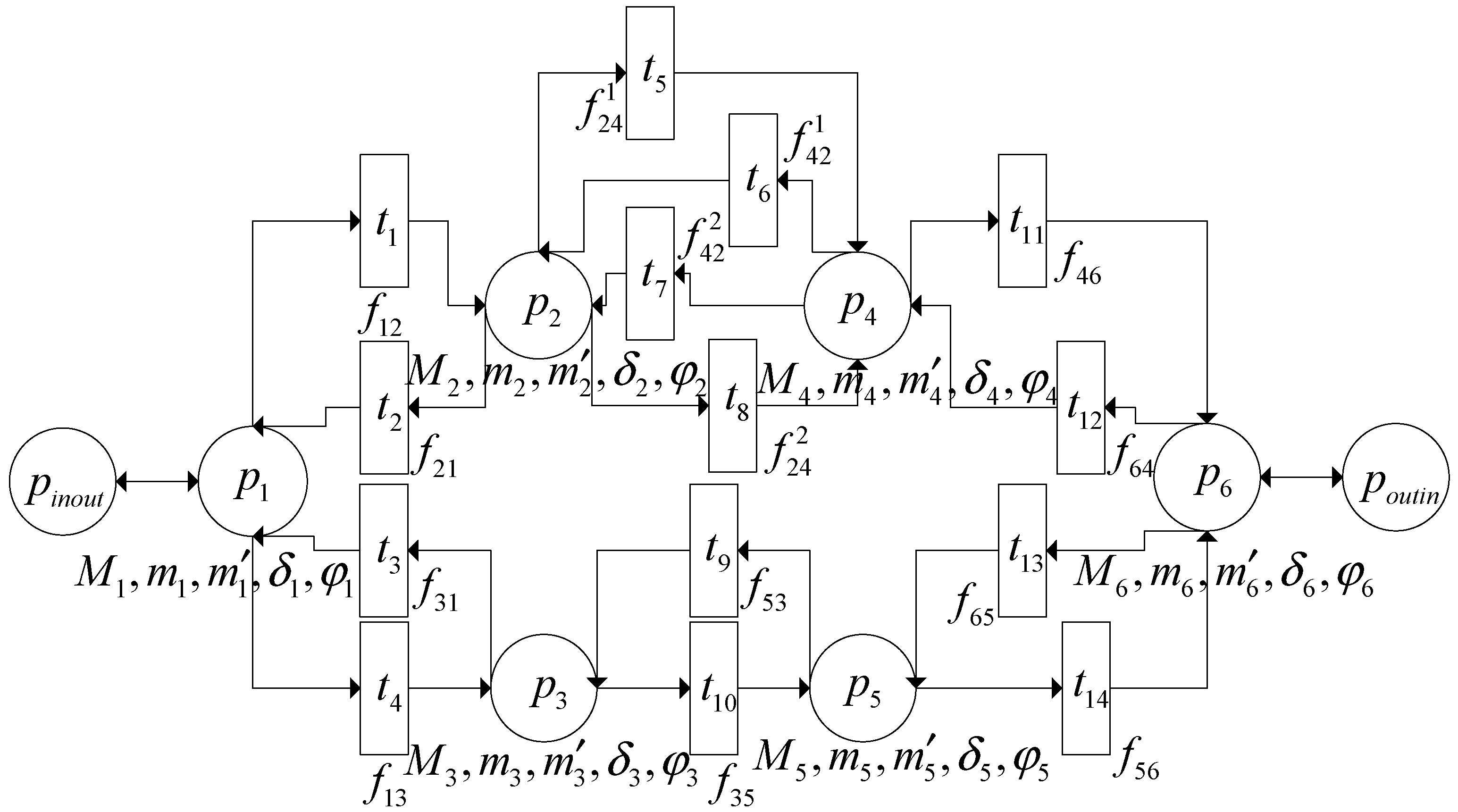
As illustrated in Figure 1, a TPN model is constructed to represent a bidirectional multi-branch tourist route structure in a scenic area. This structure integrates both multi-route and branching characteristics and provides an abstract representation of visitor flow patterns commonly observed in large-scale scenic areas. $p_{inout}$ and $p_{outin}$ denote the two entrances/exits of the scenic area. The touring direction from entrance $p_{inout}$ to exit $p_{outin}$ is defined as the forward direction, while the touring direction from $p_{outin}$ to $p_{inout}$ is defined as the reverse direction. Each attraction place $p_i$ is associated with a set of intrinsic attributes, including maximum visitor capacity $M_i$, current number of forward visitors $m_i$, current number of reverse visitors $m_i^{\prime }$, attraction weight ${\delta }_i$, and average dwell time at the attraction ${\phi }_i$. Timed transitions $t_i$ are employed to model visitors’ dwell and touring activities within attractions, while flow transitions $f_{ij}$ describe the movement of visitors between adjacent attractions. The time attributes of flow transitions represent the walking or transfer time required for visitors to move between neighboring attractions. After entering the scenic area through an entrance place $p_i$, visitors sequentially arrive at attraction places and move along the predefined touring routes. At each attraction place, visitors are required to stay for the corresponding average dwell time ${\phi }_i$ before firing the associated transition to move to the next attraction. In bidirectional touring routes, the same attraction may simultaneously receive visitor flows from different touring directions. Therefore, specific touring routes are described with respect to individual attraction places $p_i$.

By connecting all attractions in the scenic area according to the above rules, a complete bidirectional TPN model can be constructed. This bidirectional modeling approach more realistically reflects the operational characteristics of visitor flows in scenic areas with multiple entrances and exits. Based on this representation, and considering the actual spatial layout of scenic attractions, this study focuses on multi-branch and network-type touring routes. Multiple visitor guidance strategies are proposed according to the load rates of current attractions and adjacent attractions, and their operational performance is analyzed through simulation experiments. Finally, appropriate visitor guidance strategies are selected under different evaluation criteria based on relevant performance indicators, with the aim of providing scientific support for visitor management and guidance in scenic areas. It should be noted that the focus of this model is not to reproduce detailed individual behavioral heterogeneity, but to analyze congestion propagation and regulation mechanisms at the system level. Therefore, the model emphasizes network-level load dynamics and capacity-constrained flow transitions rather than micro-level behavioral realism.

3.2. Algorithmic Framework and Implementation Procedure

The preceding sections have established the TPN-based representation of visitor movement and attraction capacity constraints in the scenic-area network. Based on this modeling foundation, the next step is to integrate real-time attraction states with the model structure to support visitor guidance during peak periods.

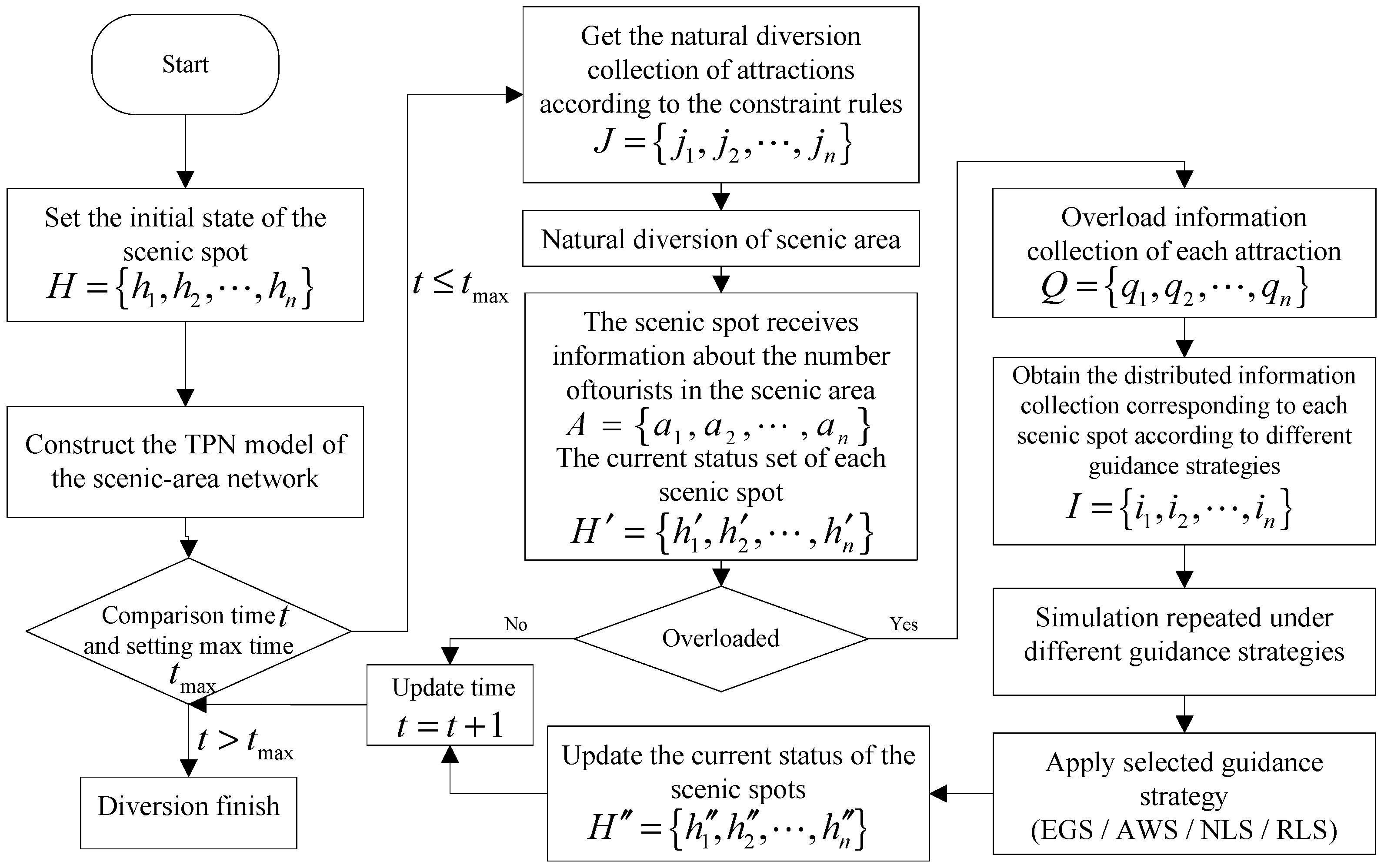
As illustrated in Figure 2, the TPN model provides the dynamic simulation framework, while the guidance strategies determine how tourists are redistributed when congestion occurs.

Within this framework, tourists enter the scenic area and their route choices are dynamically updated according to scenic spot load conditions and route structure information.

Let $H=\left\{h_1,h_2,\cdots ,h_n\right\}$ denote the set of current numbers of tourists at each scenic spot; $J=\left\{j_1,j_2,\cdots ,j_n\right\}$ denote the set of natural tourist distribution results under the absence of management intervention; $A=\left\{a_1,a_2,\cdots ,a_n\right\}$ denote the set of information on the number of tourists expected to enter the scenic area; $H^{\prime }=\left\{h_1^{\prime },h_2^{\prime },\cdots ,h_n^{\prime }\right\}$ denote the set of operational states of scenic spots after natural distribution; $Q=\left\{q_1,q_2,\cdots ,q_n\right\}$ denote the set of overload information for each scenic spot; $I=\left\{i_1,i_2,\cdots ,i_n\right\}$ denote the set of guidance information generated under different tourist guidance strategies; $H^{″}=\left\{h_1^{″},h_2^{″},\cdots ,h_n^{″}\right\}$ denote the final set of operational states of scenic spots after the implementation of real-time guidance strategies.

Through the evolution of these state sets, the model describes tourist distribution, congestion detection, and guidance implementation within a unified simulation framework.

3.3. Design of Tourist Guidance Strategies

Based on the TPN framework, a dynamic tourist guidance mechanism is embedded to regulate tourist flows during simulation. At each time step, the system monitors scenic spot loads and triggers a guidance decision once a capacity constraint is exceeded. Selected tourists are then redistributed to downstream scenic spots according to predefined rules, enabling continuous adjustment of visitor distribution during peak periods.

The guidance decisions in this study are based on different scopes of system information rather than global optimization. Here, “information coverage scope” refers to the spatial and system-state information available to the guidance strategy when making routing decisions. Depending on the strategy, the decision mechanism may rely on (i) local structural information, such as connectivity between adjacent scenic spots, (ii) local real-time state information, such as the load level of nearby attractions, or (iii) broader network-level information, such as the load conditions of paths or multiple attractions within the scenic network.

To systematically examine how different information utilization modes influence tourist guidance performance, four tourist guidance strategies are designed within the TPN-based modeling framework. These strategies are not constructed as a hierarchy of increasing complexity; instead, they represent different managerial perspectives and reflect distinct decision-making logics under varying information conditions and management assumptions.

The TPN model captures the temporal evolution of visitor flows, while the guidance strategies determine how tourists are redistributed when congestion occurs. These four strategies correspond to different information coverage scopes, ranging from purely local structural information to broader network-level state information.

Strategy 1: Equal Allocation Guidance Strategy

This strategy relies only on local structural information of the scenic area network. When congestion occurs at a scenic spot, the selected tourists for guidance are evenly distributed among all adjacent downstream scenic spots. This strategy introduces no preference or state information, assuming that all downstream scenic spots have equal priority in the guidance decision. It relies solely on the topological structure of the scenic area and represents the most basic form of local guidance with the smallest information coverage scope.

Strategy 2: Attraction-Weighted Guidance Strategy

This strategy relies on local structural information combined with predefined attraction preference information. Under this strategy, guided tourists are allocated to downstream scenic spots in proportion to their attraction weights. The attraction weight reflects a scenic spot’s popularity and tourist preference, with higher-weight spots receiving a larger proportion of guided tourists. Compared with the Equal Allocation Guidance Strategy, this approach incorporates tourist preference information, making guidance decisions more consistent with observed tourist behavior while still operating within a local information coverage scope.

Strategy 3: Load-Based Scenic Spot Guidance Strategy

This strategy utilizes local real-time state information of the scenic area system. Guided tourists are allocated based on the real-time load levels of downstream scenic spots, prioritizing spots with lower loads. Its objective is to achieve dynamic load balancing within the scenic area. By explicitly incorporating real-time system state information, this strategy extends the information coverage beyond static structural or preference information and emphasizes immediate responsiveness to current congestion conditions.

Strategy 4: Path Load-Based Guidance Strategy

Unlike the previous strategies, this approach utilizes broader network-level information, extending the guidance decision beyond individual scenic spots and evaluates the overall load levels of alternative downstream touring paths. By comparing the cumulative loads along different candidate paths, tourists are guided toward routes with lower overall congestion, thereby mitigating congestion propagation at a broader spatial scale. In this strategy, guidance decisions consider not only the load levels of adjacent scenic spots but also the operational states of subsequent scenic spots along each candidate route. Routes with lower cumulative downstream loads are regarded as having higher carrying capacity and thus receive a larger proportion of guided tourists, whereas routes with higher cumulative loads receive a reduced share. Therefore, this strategy represents the largest information coverage scope among the four strategies. Furthermore, the influence of downstream scenic spots on current guidance decisions diminishes as their temporal distance from the guidance node increases. Accordingly, a time-distance-weighted mechanism is introduced to calculate the comprehensive path load, as expressed by the following equation:

$$r_{ij}={\displaystyle \frac{{\displaystyle \sum \frac{f{k}_i}{{\tau }_i}}}{{\displaystyle \sum \frac{f}{{\tau }_i}}}}$$

(1)

Here, $r_{ij}$ represents the comprehensive load rate of scenic spot i at moment j based on the route. $f$ represents the time distance between the initial scenic spot on the route and the route node, and ${\tau }_i$ denotes the cumulative temporal distance from scenic spot i to the route decision node along the considered path. It includes both the walking time between adjacent scenic spots and the average dwell time at intermediate attractions. As ${\tau }_i$ increases, the influence generated by this scenic spot decreases, and the influence of the scenic spot on the current guidance decision gradually decreases. By computing a time-distance-weighted average of scenic spot load ratios along each path, a path-level comprehensive load indicator is obtained, which serves as the basis for determining the proportion of guided tourist flows allocated to different routes.

In summary, the four tourist guidance strategies progressively expand the scope of information utilization from local structural information to path-level operational information. This modeling approach provides a systematic basis for comparing the regulatory effectiveness of different guidance mechanisms under peak demand conditions. The differences among the four strategies in terms of information usage, management assumptions, and decision logic are summarized in

Table 4. Comparison of Four Tourist Guidance Strategies in Terms of Information Scope and Management Implications.

Guidance Strategy	Information Scope Used for Decision-Making	Type of Information	Management Implications and Applicable Scenarios
Equal allocation Guidance Strategy	Current scenic spot and its adjacent reachable scenic spots	No state information (no preference or load considered)	Serves as a baseline strategy. In the absence of detailed operational information or under weak management constraints, it provides the simplest and most direct form of tourist guidance and is used to benchmark the performance improvements of other strategies.
Attraction-Weighted Guidance Strategy	Current scenic spot and its adjacent downstream scenic spots	Static attribute information (scenic spot attraction weights)	Introduces tourist preference factors without considering real-time operational states. It is suitable for management scenarios with stable spatial structures and significant differences in scenic spot attractiveness.
Load-Based Scenic Spot Guidance Strategy	Current scenic spot and its adjacent downstream scenic spots	Dynamic operational information (composite scenic spot load ratios)	Performs local optimization based on real-time load conditions, guiding tourists away from highly loaded scenic spots. This strategy is applicable to operational environments with strict requirements for local congestion control.
Path Load-Based Guidance Strategy	Downstream touring paths originating from the current scenic spot (area/path level)	Dynamic path-level information (composite downstream path load ratios)	Evaluates future congestion risks at the path level, enabling anticipatory tourist guidance. This strategy is particularly suitable for large-scale scenic areas with complex route structures that require coordinated management across multiple scenic spots.

.

3.4. Arrival Process Modeling

To realistically capture the temporal heterogeneity of tourist arrivals during peak periods, the inbound tourist flow to the scenic area is modeled as an NHPP. Unlike homogeneous Poisson assumptions with constant arrival rates, the NHPP framework [33,34,35,36] allows the arrival intensity to vary continuously over time, which is essential for representing the pronounced concentration of tourist inflows observed during peak visiting hours.

Let $\left[t_1,t_2\right]$ denote the time interval under study. The instantaneous arrival rate is defined as a non-negative, time-dependent function $\lambda \left(t\right),t\in \left[t_1,t_2\right]$. Under the NHPP assumption, the expected number of tourists arriving during any sub-interval $\left[t_a,t_b\right]\subseteq \left[t_1,t_2\right]$ is given by $E\left[N\left(t_a,t_b\right)\right]={\displaystyle {\int }_{t_a}^{t_b}\lambda \left(t\right)dt}$.

In practice, historical visitor statistics are typically available in discrete time units (e.g., hourly counts). Let ${\widehat{\lambda }}_h$ denote the average arrival rate estimated for the $h$-th time segment $\left[t_h,t_{h+1}\right]$. To avoid discontinuities introduced by piecewise-constant arrival rates, a cubic spline interpolation is applied to the discrete observation $\left\{\left(t_h,{\widehat{\lambda }}_h\right)\right\}$, yielding a smooth approximation ${\widehat{\lambda }}_h$ over $\left[t_1,t_2\right]$. A non-negativity constraint is further imposed to ensure physical consistency, resulting in the final arrival rate function $\lambda (t)=\max \{0,\tilde{\lambda }\left(t\right)\}$.

To align with the minute-level temporal resolution of the TPN simulation, the interval $\left[t_1,t_2\right]$ is discretized using a fixed time step $\Delta t$ (set to one minute in this study). At each discrete time step $t_k=t_1+k\Delta t$, the number of newly arriving tourists is sampled as $X_k\sim Poisson\left(\lambda \left(t_k\right)\Delta t\right)$.

The resulting sequence $\left\{X_k\right\}$ serves as the external input to the dynamic simulation, driving the evolution of tourist distribution and triggering potential congestion and guidance interventions.

This arrival modeling approach provides a consistent interface between empirical visitor statistics and the time-driven simulation framework, enabling the reproduction of peak-period arrival dynamics while maintaining compatibility with the minute-level decision mechanisms embedded in the TPN model.

The parameter settings used in the simulation are derived from available historical visitor statistics and spatial capacity calculations. Due to the absence of minute-level trajectory data, the NHPP-based modeling approach provides a practical method for approximating peak-period visitor arrivals at the temporal resolution required by the simulation. These hourly statistics are converted into a time-dependent arrival intensity function and discretized into minute-level intervals to support the time-driven simulation. Although attraction-level historical load profiles were not available for direct validation, the simulated baseline preserves the empirically observed temporal concentration of visitor arrivals during the holiday peak period derived from historical entrance statistics.

3.5. Experimental Evaluation Metrics

To comprehensively assess the natural dispersion scenario and the four proposed visitor guidance strategies, the primary evaluation metrics include the average scenic area load rate, TS, and the variance of scenic spot load rates. These indicators characterize overall operational pressure, visitor experience quality, and the degree of load balance among scenic spots, respectively.

3.5.1. Scenic Area Performance Metrics

(1) Average Load Rate

At time step j, the load rate of visitors at scenic spot i is defined as:

$$l_{ij}={\displaystyle \frac{m_{ij}+m_{ij}^{\prime }}{M_i}}$$

(2)

where $m_{ij}$ and $m_{ij}^{\prime }$ denote the numbers of forward- and reverse-direction visitors at scenic spot i at time j, respectively; $M_i$ represents the maximum visitor capacity of scenic spot i; and $l_{ij}$ denotes the load rate of scenic spot i at time j.

Accordingly, the vacancy (idle) rate $e_{ij}$ is defined as:

$$e_{ij}=1-l_{ij}$$

(3)

where $e_{ij}$ denotes the vacancy rate of scenic spot i at time j.

The average scenic area load rate is calculated as:

$$L_{ave}={\displaystyle \sum {\omega }_i{l}_{ij}}$$

(4)

where ${\omega }_i$ denotes the weight of scenic spot i, reflecting its relative importance within the scenic area. This indicator represents the weighted average load level of all scenic spots in the scenic area at time j.

(2) Load Rate Variance

The variance of scenic spot load rates is defined as:

$$E_{ij}={\left(l_{ij}-L_{ave}\right)}^2$$

(5)

A smaller value indicates a more balanced load distribution among scenic spots at time j.

(3) Tourism Satisfaction

Tourism satisfaction is also closely related to perceived crowding conditions, and at time j, the TS at scenic spot i is defined as:

$$s_{ij}=\alpha e_{ij}{m}_{ij}{\omega }_i$$

(6)

where $s_{ij}$ denotes the TS at scenic spot i at time j; $e_{ij}$ represents the vacancy rate of scenic spot i; $\alpha$ is a positive coefficient indicating the strength of the positive correlation between TS and vacancy rate $e_{ij}$; $m_{ij}$ denotes the total number of visitors at scenic spot i at time j; and ${\omega }_i$ represents the weight of scenic spot i. To improve clarity, the variables involved in Equation (6) are summarized in

Table 5. Explanation of Variables in the Tourist Satisfaction Model.

Symbol	Description
$s_{ij}$	Tourist satisfaction level at scenic spot i during time step j
$e_{ij}$	Vacancy rate of scenic spot i at time step j, representing the proportion of unused carrying capacity
$m_{ij}$	Number of tourists present at scenic spot i during time step j
${\omega }_i$	Attraction weight of scenic spot i, representing its relative popularity or importance
$\alpha$	Positive coefficient controlling the influence of vacancy rate on satisfaction
i	Index of scenic spots in the scenic area network
j	Simulation time step

.

In this formulation, the vacancy rate reflects the spatial availability of scenic spots, while the number of tourists represents the scale of visitor activity. Their interaction allows the satisfaction indicator to capture the trade-off between congestion pressure and recreational atmosphere.

This metric $s_{ij}$ integrates both scenic spot attributes and visitor-related factors. $e_{ij}{\omega }_i$ is the product of the vacancy rate and the weight of each scenic spot. Specifically, TS increases with higher vacancy rates, but is also influenced by the number of visitors present $m_{ij}$. When the number of visitors $m_{ij}$ is low, a high vacancy rate yields high individual satisfaction, yet the overall satisfaction level remains limited. As visitor numbers increase, vacancy rates $s_{ij}$ decrease while overall satisfaction initially rises, reaching a peak, and then declines as congestion intensifies. This inverted U-shaped relationship is consistent with real-world visitor experience patterns in scenic areas.

3.5.2. Statistical Evaluation Methods

(1) Mean-Dispersion Analysis

To systematically evaluate the overall performance of different visitor guidance strategies in terms of operational efficiency, visitor experience, and system stability, a mean–dispersion analysis is conducted from both average performance and fluctuation characteristics. Beyond traditional mean–dispersion analysis, a random seed dimension is introduced to distinguish the effects of temporal fluctuations and stochastic disturbances on system performance.

Let the time series of a given evaluation metric under guidance strategy i and random seed k over the simulation horizon be denoted as:

$${\chi }_{i,k}=\left\{\left.X_{i,k}\left(t\right)\right|t=1,2,\dots ,T\right\}$$

(7)

where $i=1,2,\dots ,I$ denotes the guidance strategy index, $k=1,2,\dots ,K$ denotes the random seed index, and $T$ represents the total number of simulation time steps (minutes).

(2) Time-Level Mean and Dispersion under a Fixed Random Seed

Under a fixed random seed k, the time-averaged value of strategy i is defined as:

$${\overline{X}}_{i,k}={\displaystyle \frac{1}{T}}{\displaystyle \sum _{t=1}^T{X}_{i,k}\left(t\right)}$$

(8)

The corresponding temporal dispersion (standard deviation) is defined as:

$${\sigma }_{i,k}=\sqrt{{\displaystyle \frac{1}{T}}{\displaystyle \sum _{t=1}^T{\left(X_{i,k}\left(t\right)-{\overline{X}}_{i,k}\right)}^2}}$$

(9)

These indicators describe the average performance level and temporal variability of strategy i under a specific stochastic arrival realization.

(3) Cross-Seed Mean Aggregation

To mitigate the influence of single random realizations, the time-averaged values across different random seeds are aggregated to define the cross-seed average performance:

$${\overline{X}}_i^{\left(seed\right)}={\displaystyle \frac{1}{K}}{\displaystyle \sum _{t=1}^T{\overline{X}}_{i,k}}$$

(10)

This indicator reflects the overall average performance of guidance strategy i under different stochastic conditions.

(4) Cross-Seed Dispersion

To evaluate the sensitivity of strategy performance to stochastic disturbances, the cross-seed dispersion of the mean performance is defined as:

$${\sigma }_i^{\left(seed\right)}=\sqrt{{\displaystyle \frac{1}{K}}{\displaystyle \sum _{k=1}^K{\left({\overline{X}}_{i,k}-{\overline{X}}_i^{\left(seed\right)}\right)}^2}}$$

(11)

A smaller value indicates that the strategy is less sensitive to stochastic disturbances and exhibits stronger robustness.

(5) Two-Level Mean-Dispersion Framework

By integrating the time dimension and the random seed dimension, a two-level analytical framework is constructed. At the time level, ${\overline{X}}_{i,k}$ and ${\overline{X}}_{i,k}$ describe system dynamics within a single simulation run; at the random level, ${\overline{X}}_i^{\left(seed\right)}$ and ${\sigma }_i^{\left(seed\right)}$ characterize the overall stability of strategy performance under stochastic perturbations. This framework effectively distinguishes between temporal variability and stochastic uncertainty, providing a foundation for robustness evaluation and comprehensive strategy assessment.

(6) Statistical Distribution Analysis

To further characterize the distributional properties of evaluation metrics across time and stochastic conditions, boxplot analysis is employed. Boxplots depict central tendencies, dispersion, and extreme fluctuations using quantile information, serving as an important complement to mean-dispersion analysis.

(7) Robustness Evaluation Metrics

To quantitatively assess the stability of the TS-ALR relationship under different stochastic conditions, a robustness evaluation framework is constructed based on three indicators: optimal load rate deviation $D_{\rho ,s}$, optimal satisfaction fluctuation $D_{S,s}$, and satisfaction-load curve consistency $D_{C,s}$. If a visitor guidance strategy simultaneously exhibits small optimal load rate deviation, low optimal satisfaction fluctuation, and high curve consistency, the TS-ALR relationship under that strategy is considered robust and insensitive to stochastic disturbances. By introducing the random seed dimension, the traditional mean-dispersion analysis across different information coverage scopes is extended into a two-level statistical framework, enabling a comprehensive evaluation of visitor guidance strategies from both temporal fluctuation and stochastic disturbance perspectives.

In subsequent analyses, minute-level time series and statistical characteristics are jointly examined to systematically compare the performance of different guidance strategies, providing quantitative support for experimental result interpretation and strategy evaluation. The pseudocode of the proposed dynamic visitor guidance model is provided in Appendix C (Algorithm A1) to clarify the algorithmic workflow of the model.

4. Experimental Setup

4.1. Scenic Area Spatial Structure and Scenic Spot Modeling

To examine the effectiveness of the proposed TPN-based dynamic visitor guidance model and the associated guidance strategies, Mount Huangshan Scenic Area is selected as the case study for simulation experiments. Mount Huangshan is a typical mountainous tourist destination, characterized by a wide spatial distribution of scenic spots, complex touring routes, and highly concentrated visitor flows during holidays and peak tourism seasons. As a result, significant congestion frequently occurs at several key nodes, making it a representative and suitable case for studying peak-period visitor management.

Mount Huangshan features multi-branching and network-type routes, heterogeneous scenic spots, and bidirectional visitor movements between different entrances and exits. These characteristics make it a suitable case for evaluating the proposed bidirectional visitor guidance model and multi-strategy guidance mechanisms.

In the simulation experiments, the spatial structure of the scenic area is appropriately abstracted and simplified based on the main touring routes and core scenic spots of Mount Huangshan. While preserving key topological characteristics and functional nodes, a scenic area network model for simulation is constructed to achieve a balance between model fidelity and computational feasibility.

According to the actual touring layout of Mount Huangshan and the primary activity paths of visitors, several representative core scenic spots are selected as nodes in the model. The major accessibility relationships between scenic spots are abstracted as directed connections, thereby forming the topological structure of the scenic area used in the simulation analysis.

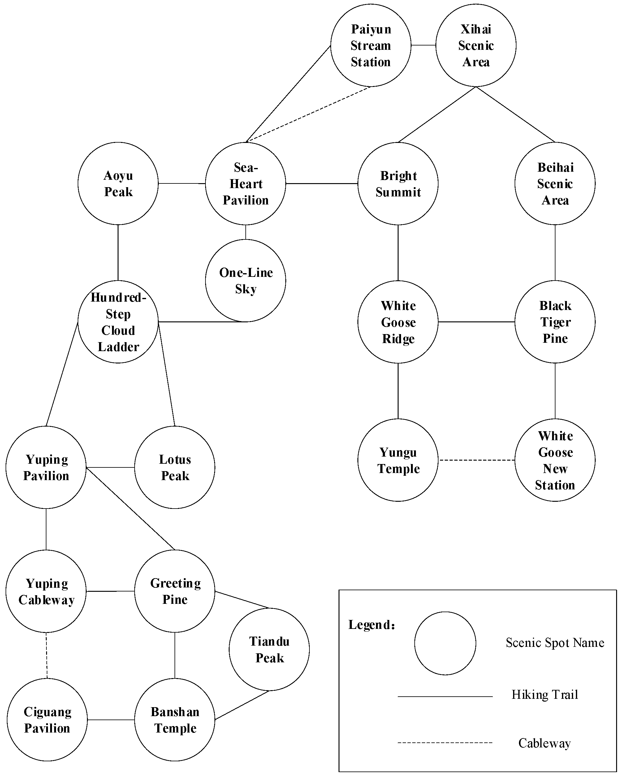
As shown in Figure A1, a simplified spatial distribution map of Mount Huangshan Scenic Area is constructed for the simulation experiments. The model explicitly considers visitor capacity and load variation at each scenic spot, while pathway throughput capacity is not modeled separately.

Certain secondary scenic spots along the same route are not modeled as independent nodes; instead, their influence is represented by adjusting the attraction weights of adjacent core scenic spots. This preserves route preference characteristics while keeping the network structure concise.

4.2. Scenic Spot Parameters and Visitor Behavior Settings

In the simulation experiments, each scenic spot is assigned a set of parameters, including scenic spot capacity, attraction weight, and average visiting time. Scenic spot capacity represents the maximum number of visitors that the spot can accommodate, serving as the primary constraint for load management. Attraction weight reflects the relative attractiveness of the spot in the visitor choice process, influencing the proportion of visitors directed toward it. Average visiting time describes the average duration a visitor spends at the scenic spot, which determines the timing of transitions between spots.

4.2.1. Modeling of Scenic Spots

Each scenic spot in the model is abstracted as a node with associated capacity and temporal attributes. The combination of these parameters, along with the attraction weights, allows the simulation to capture visitor accumulation, flow dynamics, and the effect of guidance strategies on both individual spots and the overall network.

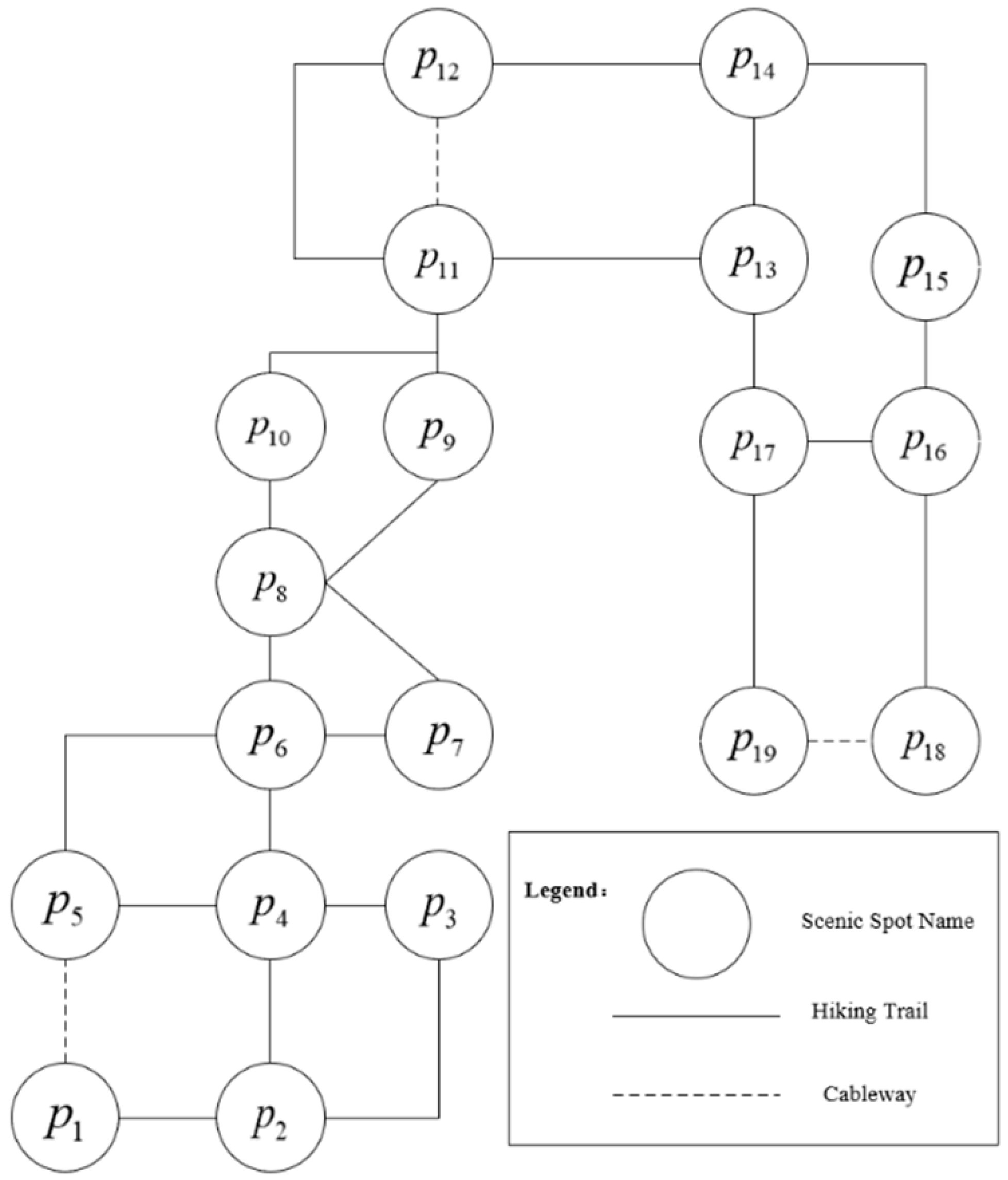
After determining the scenic area touring routes and scenic spot structure (Figure A1), the scenic spots within the scenic area are further modeled and parameterized for the simulation. Figure A2 presents the numbered touring routes of scenic spots in Mount Huangshan Scenic Area.

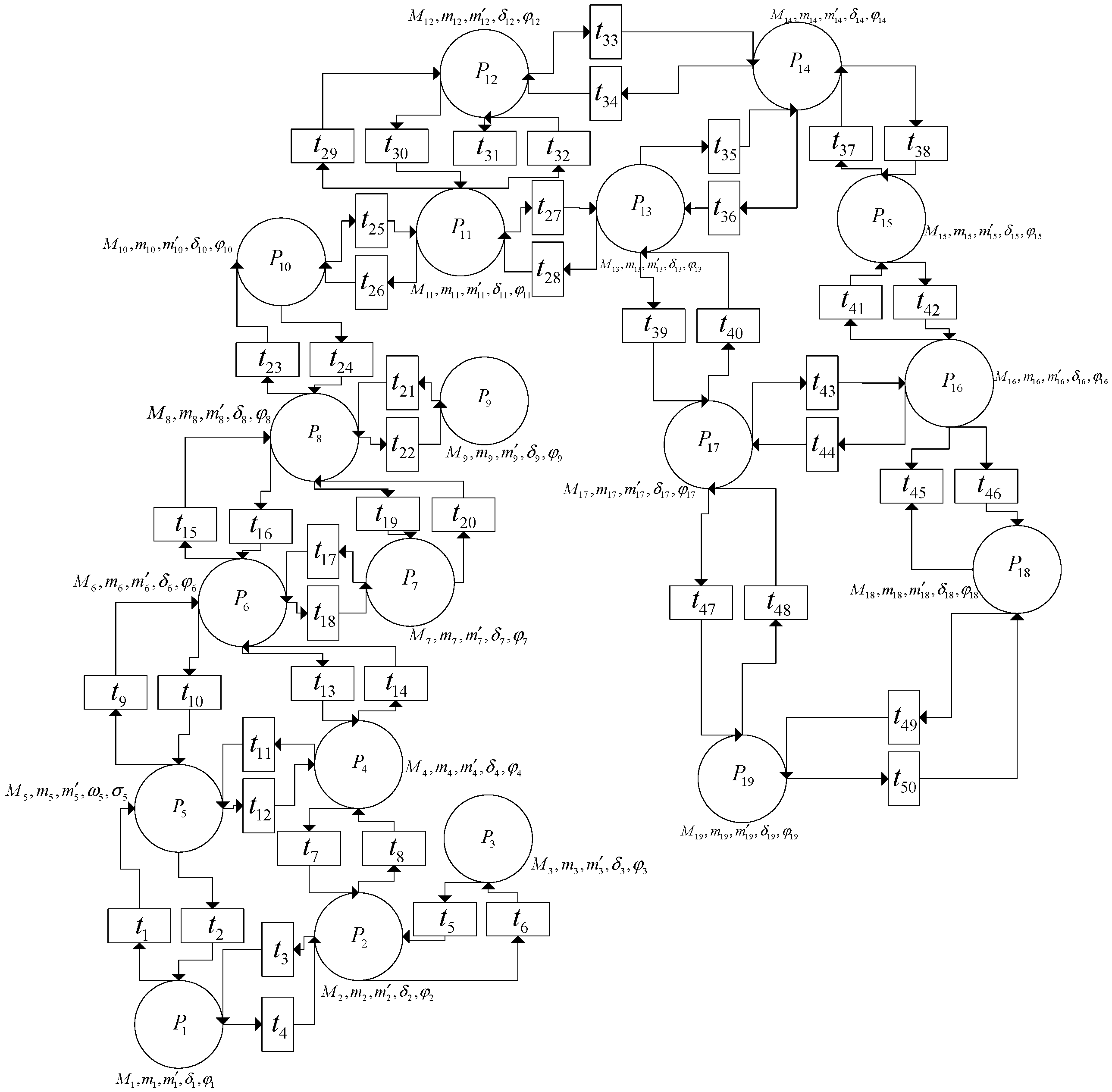
Based on this routing configuration, a TPN-based bidirectional visitor guidance touring network for Mount Huangshan during peak periods is constructed. This network provides the structural foundation for simulating bidirectional visitor movements and evaluating the performance of different visitor guidance strategies under high-demand conditions.

As shown in Figure 3, $p_i,i=1,2,\cdots ,19$ denotes each scenic spot, while $p_1$ and $p_{19}$ represent the entrances and exits of the scenic area, respectively. $M_i,i=1,2,\cdots ,19$ denotes the maximum carrying capacity of scenic spot $p_i$; $m_i,m_i^{\prime },i=1,2,\cdots ,19$ denote the numbers of visitors touring in the forward and reverse directions, respectively; ${\delta }_i,i=1,2,\cdots ,19$ represents the attraction weight of scenic spot $p_i$; and ${\phi }_i,i=1,2,\cdots ,19$ denotes the average visiting (dwelling) time at scenic spot $p_i$.

Visitor movements within the scenic area are classified into forward and reverse touring directions. Visitors enter the scenic area from one entrance and eventually exit from another entrance, without revisiting the same scenic spot during the tour. When multiple feasible paths exist between two adjacent scenic spots, visitors randomly select among the available paths under connectivity constraints. The specific path choice behavior is jointly influenced by the applied visitor guidance strategy and stochastic factors.

4.2.2. Simulation Time Scale and Virtual Clock Configuration

The configuration of the virtual clock in the simulation should be consistent with the temporal distribution characteristics of real visitor flows [37,38]. Based on the analysis of visitor flow patterns in Mount Huangshan Scenic Area, daily visitor peaks are primarily concentrated between 08:00 and 12:00, lasting approximately 4 h. During this period, visitor numbers at certain scenic spots may exceed their carrying capacities, whereas the overall system remains relatively stable during off-peak periods. Accordingly, the simulation time horizon is set to 240 min, corresponding to the complete peak-period window. To capture the dynamic evolution of visitor movements and real-time guidance decisions, the virtual clock advances in discrete time steps of 1 min. At each time step, the visitor distribution across scenic spots is updated, and the corresponding guidance decisions are executed. This minute-level dynamic simulation environment enables an in-depth analysis of the real-time regulation effects of different visitor guidance strategies under peak-period conditions.

4.2.3. Attraction Weight Parameter Settings of Scenic Spots

As shown in Figure 3, after simplifying and screening the scenic spots in the Huangshan Scenic Area, a total of 19 scenic spots are ultimately selected as research objects for the dynamic simulation experiments. To characterize the differences in attractiveness among scenic spots in tourists’ route selection behavior, attraction weight parameters are assigned to each scenic spot based on their popularity and actual visitation intensity. Specifically, highly representative core attractions in the Huangshan Scenic Area (e.g., Yingke Pine) are assigned the highest weight of 0.10. Well-known scenic spots such as Tiandu Peak, Lotus Peak, One-Line Sky, Bright Summit, and West Sea are assigned a relatively high weight of 0.07, while all remaining scenic spots are uniformly assigned a lower weight of 0.03. These weight settings are intended to reflect the relative differences in tourists’ preferences for different scenic spots. The specific weight values for each scenic spot are listed in

Table A1. Attraction Weights of Scenic Spots in the Huangshan Scenic Area.

Scenic Spot	Ciguang Pavilion	Banshan Temple	Tiandu Peak	Greeting Pine	Yuping Cableway	Yuping Pavilion	Lotus Peak	Hundred-Step Cloud Ladder	One-Line Sky	Aoyu Peak
Weight	0.03	0.03	0.07	0.1	0.03	0.07	0.07	0.03	0.07	0.07
Scenic Spot	Sea-Heart Pavilion	Paiyun Stream Station	Bright Summit	Xihai	Beihai	Black Tiger Pine	White Goose Ridge	White Goose New Station	Yungu Temple
Weight	0.03	0.03	0.07	0.07	0.07	0.07	0.03	0.03	0.03

.

4.2.4. Time Distance Between Upstream and Downstream Scenic Spots

Based on the determined distances between scenic spots, and in combination with data provided in previous studies and by the Huangshan Scenic Area Administrative Committee, the distances between scenic spots are obtained and presented in

Table A2. Inter-Attraction Distances in Huangshan Scenic Area.

Link Origin	Link Destination	Length (m)	Link Origin	Link Destination	Length (m)
Ciguang Pavilion	Banshan Temple	2050	One-Line Sky	Sea-Heart Pavilion	580
Ciguang Pavilion	Yuping Cableway	2010	Sea-Heart Pavilion	Paiyun Stream Station	[3000,3560]
Banshan Temple	Tiandu Peak	1050	Sea-Heart Pavilion	Bright Summit	200
Banshan Temple	Greeting Pine	1005	Paiyun Stream Station	Xihai Scenic Area	2000
Tiandu Peak	Greeting Pine	1050	Bright Summit	Xihai Scenic Area	1500
Greeting Pine	Yuping Cableway	150	Xihai Scenic Area	Beihai Scenic Area	500
Greeting Pine	Yuping Pavilion	105	Bright Summit	White Goose Ridge	600
Yuping Cableway	Yuping Pavilion	100	Beihai Scenic Area	Black Tiger Pine	250
Yuping Pavilion	Lotus Peak	500	White Goose Ridge	Black Tiger Pine	250
Yuping Pavilion	Hundred-Step Cloud Ladder	680	Black Tiger Pine	White Goose New Station	1030
Hundred-Step Cloud Ladder	One-Line Sky	180	White Goose Ridge	Yungu Temple	3450
Hundred-Step Cloud Ladder	Aoyu Peak	200	Yungu Temple	White Goose New Station	2700
Aoyu Peak	Sea-Heart Pavilion	600

(Appendix A).

Tourists travel between scenic spots in the Huangshan Scenic Area mainly by walking and cableways, with cableways covering only certain fixed routes within the scenic area. For example, Yuping Cableway–Ciguang Pavilion and Yungu Temple–White Goose New Station are directly connected by cableways. In contrast, between Haixin Pavilion and Paiyunxi Station, both cableway routes and mountain walking paths exist. Therefore, during the modeling process, distances for cableway routes and walking paths are recorded separately.

To further calculate tourists’ travel time along different paths, spatial distances are converted into time distances by considering tourists’ walking speed and the operating speeds of cableways and gondolas. In real-world scenic area operations, tourists’ walking speeds are influenced by multiple factors, including mountainous terrain, slope variations between scenic spots, differences in path width, and weather conditions. Moreover, on the same path, ascending and descending tourists typically exhibit significantly different movement speeds. For cableways and gondolas, operating speeds also vary across different lines (e.g., Yuping Cableway, Yungu Cableway, and West Sea Grand Canyon Sightseeing Cable Car).

To emphasize the effects of tourist guidance strategies on scenic area operations during peak periods, and to avoid introducing excessive confounding factors weakly related to the research objectives, a set of unified assumptions is adopted in the simulation experiments. Specifically, all inter-spot pathways are assumed to have identical widths; all tourists are assigned a constant walking speed regardless of ascending or descending direction; and the operating speeds of all cableways and gondolas are treated as constant. Under these assumptions, tourists’ walking speed is set to 30 m/min, and the operating speed of cableways and gondolas is set to 420 m/min, which are used to calculate the time distance parameters between scenic spots.

After determining the distances between scenic spots and the corresponding travel speeds, the time distance between any two scenic spots can be calculated using the following formula:

$$f_{ij}={\displaystyle \frac{d_{ij}}{v_t}}$$

(12)

where $f_{ij}$ denotes the time distance between scenic spots i and j, $d_{ij}$ represents the actual spatial distance between them, and $v_t$ denotes the travel speed. When $t=1$, $v_t$ corresponds to tourists’ walking speed; when $t=2$, it represents the speed of cableways or gondolas. Based on the above parameters, the time distances between scenic spots are calculated accordingly. For ease of discrete-time simulation, the calculated time distances are rounded to the nearest integer to obtain the final time distance parameters used in the simulation. It should be noted that if no direct connection exists between two scenic spots, their time distance is set to 0. The final time distance values between all scenic spots are listed in

Table A3. Travel Time Between Attractions in the Huangshan Scenic Area.

	Ciguang Pavilion	Banshan Temple	Tiandu Peak	Greeting Pine	Yuping Cableway	Yuping Pavilion	Lotus Peak	Hundred-Step Cloud Ladder	One-Line Sky	Aoyu Peak
Ciguang Pavilion	0	68	0	0	5	0	0	0	0	0
Banshan Temple	68	0	35	34	0	0	0	0	0	0
Tiandu Peak	0	35	0	35	0	0	0	0	0	0
Greeting Pine	0	34	35	0	5	4	0	0	0	0
Yuping Cableway	5	0	0	5	0	3	0	0	0	0
Yuping Pavilion	0	0	0	4	3	0	17	23	0	0
Lotus Peak	0	0	0	0	0	17	0	20	0	0
Hundred-Step Cloud Ladder	0	0	0	0	0	23	20	0	6	7
One-Line Sky	0	0	0	0	0	0	0	6	0	0
Aoyu Peak	0	0	0	0	0	0	0	7	0	0
Sea-Heart Pavilion	0	0	0	0	0	0	0	0	19	20
Paiyun Stream Station	0	0	0	0	0	0	0	0	0	0
Bright Summit	0	0	0	0	0	0	0	0	0	0
Xihai Scenic Area	0	0	0	0	0	0	0	0	0	0
Beihai Scenic Area	0	0	0	0	0	0	0	0	0	0
Black Tiger Pine	0	0	0	0	0	0	0	0	0	0
White Goose Ridge	0	0	0	0	0	0	0	0	0	0
White Goose New Station	0	0	0	0	0	0	0	0	0	0
Yungu Temple	0	0	0	0	0	0	0	0	0	0
	Sea-Heart Pavilion	Paiyun Stream Station	Bright Summit	Xihai Scenic Area	Beihai Scenic Area	Black Tiger Pine	White Goose Ridge	White Goose New Station	Yungu Temple
Ciguang Pavilion	0	0	0	0	0	0	0	0	0
Banshan Temple	0	0	0	0	0	0	0	0	0
Tiandu Peak	0	0	0	0	0	0	0	0	0
Greeting Pine	0	0	0	0	0	0	0	0	0
Yuping Cableway	0	0	0	0	0	0	0	0	0
Yuping Pavilion	0	0	0	0	0	0	0	0	0
Lotus Peak	0	0	0	0	0	0	0	0	0
Hundred-Step Cloud Ladder	0	0	0	0	0	0	0	0	0
One-Line Sky	19	0	0	0	0	0	0	0	0
Aoyu Peak	20	0	0	0	0	0	0	0	0
Sea-Heart Pavilion	0	[7,119]	7	0	0	0	0	0	0
Paiyun Stream Station	[7,119]	0	0	67	0	0	0	0	0
Bright Summit	7	0	0	50	0	0	20	0	0
Xihai Scenic Area	0	67	50	0	17	0	0	0	0
Beihai Scenic Area	0	0	0	17	0	8	0	0	0
Black Tiger Pine	0	0	0	0	8	0	8	34	0
White Goose Ridge	0	0	20	0	0	8	0	14	115
White Goose New Station	0	0	0	0	0	34	14	0	6
Yungu Temple	0	0	0	0	0	0	115	6	0

(Appendix A).

4.2.5. Average Visiting Time of Scenic Spots

The average visiting time of each scenic spot is determined based on its popularity and typical tourist stay characteristics observed in actual visits. Considering typical tourist behaviors across different scenic spots in the Huangshan Scenic Area, the average visiting time for each scenic spot is uniformly set within the range of 5–10 min, with specific values shown in

Table A4. Average Visiting Time of Scenic Spots.

Scenic Spot	Ciguang Pavilion	Banshan Temple	Tiandu Peak	Greeting Pine	Yuping Cableway	Yuping Pavilion	Lotus Peak	Hundred-Step Cloud Ladder	One-Line Sky	Aoyu Peak
Time	5	5	10	10	5	10	10	5	8	8
Scenic Spot	Sea-Heart Pavilion	Paiyun Stream Station	Bright Summit	Xihai	Beihai	Black Tiger Pine	White Goose Ridge	White Goose New Station	Yungu Temple
Time	5	10	10	10	10	5	5	5	5

. This setting is intended to reflect relative differences in tourists’ dwell times across scenic spots while avoiding the introduction of overly fine-grained individual-level heterogeneity.

It should be noted that during model construction, the entrance and exit points of the scenic area (i.e., Ciguang Pavilion and Yungu Temple) are also treated as functional scenic spot nodes and are assigned corresponding visiting times to capture potential tourist stopping and aggregation behaviors during entry and exit processes. In addition, although the West Sea Grand Canyon is characterized by a long and continuous touring route in the actual scenic area, it is abstracted as a single scenic spot in the model to facilitate load-based tourist guidance and diversion experiments.

4.2.6. Maximum Carrying Capacity of Scenic Spots

In scenic area management and tourist flow studies, the maximum carrying capacity of a scenic spot generally refers to the maximum number of tourists that a scenic spot can accommodate or allow to pass within a given time scale, without inducing safety risks, significantly degrading visitor experience, and while remaining manageable by the operational system. The classification of tourist spatial safety density in this study draws on density-based risk assessment methods from crowd safety and event safety management, in which different crowd density levels correspond to different spatial states and safety risk levels [39,40]. Considering the characteristics of mountainous scenic areas, a tourist safety density classification framework suitable for the Huangshan Scenic Area is established (

Table A5. Classification of Tourist Spatial Safety Density and Applicability to Scenic Areas.

Safety Density	State Description	Safety Assessment	Applicability to Scenic Areas
≤0.5	Very spacious	Extremely safe	Recommended (especially suitable for mountainous scenic areas)
0.5–1.0	Comfortable and controllable	Safe	Recommended
1.0–2.0	Crowded but still mobile	Marginally safe	Use with caution; suitable only for short-term transitions
2.0–4.0	Obviously crowded	Unsafe	Not recommended
≥4.0	Highly dangerous	Extremely unsafe	Prohibited

).

An area–density method is employed to calculate the upper limit of scenic spot carrying capacity, defined as the product of the effective activity area of a scenic spot and the corresponding safety density. For scenic spot i, the carrying capacity is defined as:

$$M_i=A_i\times s{d}_i,i=1,2,\cdots ,n$$

(13)

where $A_i$ denotes the effective activity area of scenic spot i, $s{d}_i$ represents the safety density corresponding to the spatial type, and $M_i$ is the maximum allowable tourist capacity of scenic spot i.

Table A5 presents the general classification standards for tourist spatial safety density, which are derived from the dynamic analyses of crowd behavior and density in Still’s doctoral dissertation Crowd Dynamics [41], as well as the comprehensive framework on density risk and management proposed in Introduction to Crowd Science [39]. In this study, crowd density refers to the average number of tourists per unit of effective activity area. For mountainous scenic areas, which are characterized by steep terrain, narrow pathways, and numerous exposed sections, more conservative safety density standards are adopted compared to urban public spaces. In the modeling and simulation experiments, 0.5–1.0 persons/m² is regarded as the safe operating range, with 1.0 persons/m² taken as the upper safety limit. The effective activity areas of scenic spots are measured based on layout drawings provided by the Huangshan Scenic Area Administrative Committee. The final carrying capacity values are calculated using Equation (13) and are presented in

Table A6. Maximum Tourist Carrying Capacity of Scenic Spots in the Huangshan Scenic Area.

Scenic Spot	Ciguang Pavilion	Banshan Temple	Tiandu Peak	Greeting Pine	Yuping Cableway	Yuping Pavilion	Lotus Peak	Hundred-Step Cloud Ladder	One-Line Sky	Aoyu Peak
Max $M_i$	50	50	50	40	40	40	40	20	25	25
Scenic Spot	Sea-Heart Pavilion	Paiyun Stream Station	Bright Summit	Xihai	Beihai	Black Tiger Pine	White Goose Ridge	White Goose New Station	Yungu Temple
Max $M_i$	25	40	40	50	100	30	30	50	50

.

4.2.7. Initial Tourist Population Settings

To account for the pronounced concentration of tourists during public holidays, historical inbound flow data for the Huangshan Scenic Area between 8:00 and 11:00 were used to estimate the initial tourist population. After averaging, the hourly inbound tourist volumes were 3239, 2946, 2408, and 1657, respectively. A discretized NHPP was then employed to model the initial tourist scale and arrival process in the simulation experiments.

4.3. Implementation Environment and Runtime

The simulation framework was implemented in Python (version 3.12.7). The implementation relies on commonly used scientific computing libraries, including NumPy and Pandas for numerical computation and data processing, and Matplotlib for visualization.

All experiments were conducted on a workstation equipped with an Intel Core i5-12600KF CPU and 32 GB RAM running the Windows operating system.

Since the proposed Timed Petri Net (TPN) model operates at an aggregated visitor-flow level rather than simulating individual agents, the computational complexity remains relatively low. Under the experimental configuration used in this study, each simulation scenario typically completes within approximately 5–10 s.

This computational efficiency enables repeated simulations under different guidance strategies and random arrival conditions.

5. Results and Analysis

Based on the modeling of tourist flows, parameter settings, and the design of tourist guidance strategies, simulation experiments were further conducted to systematically analyze the operational performance of the scenic area under the natural dispersion scenario and four guided scenarios. The simulations were implemented in a Python environment. Under unified random conditions, minute-level dynamic simulations were performed to reproduce tourist movements during peak periods in Huangshan Scenic Area. The regulation effects of different tourist guidance strategies were evaluated from three key dimensions: operational efficiency of the scenic area, tourist experience, and system stability.

5.1. Operational Characteristics Under the Natural Dispersion Scenario

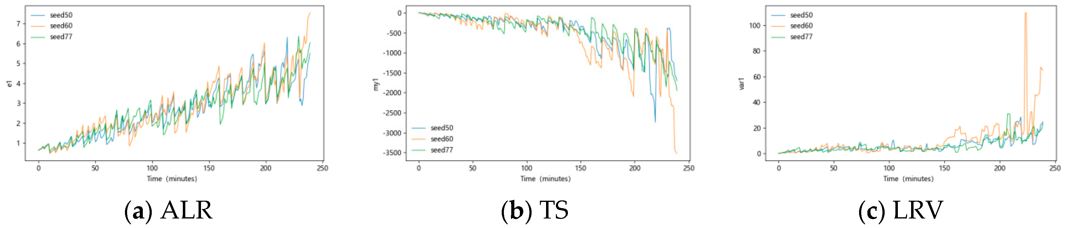
This subsection first examines the natural dispersion scenario without the adoption of any tourist guidance strategy, which serves as the baseline for subsequent comparative analyses. As illustrated in Figure 4, which depicts the temporal evolution of key performance indicators under the natural dispersion scenario, the simulation results indicate that during peak periods, the ALR of the scenic area remains at a relatively high level under natural dispersion and exhibits pronounced temporal fluctuations. Several key attractions experience sustained overload conditions across multiple time steps.

Meanwhile, TS demonstrates significant instability over time, with sharp declines observed in certain periods, indicating that tourist experience is highly sensitive to the accumulation of localized congestion.

From a spatial perspective, the variance of the ALR across attractions remains consistently high under the natural dispersion scenario, revealing a highly uneven distribution of tourist loads among attractions. Substantial disparities are observed between hotspot attractions and non-hotspot ones. These findings suggest that, in the absence of proactive intervention, random tourist arrivals and unguided path selection behaviors tend to amplify congestion accumulation, resulting in poor overall operational quality and low system stability of the scenic area.

5.2. Overall Performance Evaluation of Tourist Guidance Strategies

Building upon the natural dispersion baseline, tourist guidance strategies are introduced to conduct an overall evaluation of the scenic area’s operational performance. The statistical results indicate that, compared with the natural dispersion scenario, the implementation of tourist guidance strategies leads to significant improvements across all three core indicators, namely the ALR of the scenic area, TS, and the variance of the ALR.

Table 6. Overall Differences before and after the Implementation of Tourist Guidance Strategies.

Indicator	Natural Dispersion		Pre-Guidance		Post-Guidance		Change vs. Natural Dispersion		Change vs. Pre-Guidance
	Mean	Std. Dev.	Mean	Std. Dev.	Mean	Std. Dev.	Mean	Std. Dev.	Mean	Std. Dev.
ALR	2.6782	1.3983	0.7168	0.1240	0.6911	0.0974	−74.20%	−93.03%	−3.58%	−21.8%
TS	−491.4920	519.2309	5.0056	2.0331	7.4221	0.4923	−101.51%	−99.91%	+48.25%	−75.8%
LRV	7.3748	9.4308	0.0823	0.0484	0.0316	0.0267	−99.75%	−99.72%	−61.55%	−45.0%

presents the overall statistical differences before and after the implementation of tourist guidance strategies. Specifically, the ALR of the scenic area decreases markedly, indicating that the guidance mechanisms effectively suppress the continuous accumulation of visitor loads in local areas. TS increases substantially, rising from extremely low levels under natural dispersion to a stable positive range, which reflects a systematic improvement in the overall tourist experience. Meanwhile, the variance of the ALR shows a clear convergence trend, suggesting that the internal load distribution across scenic spots becomes more balanced and that the overall system stability is significantly enhanced.

These results indicate that visitor guidance improves not only average system performance but also overall operational stability during peak periods.

5.3. Comparative Analysis of Different Visitor Guidance Strategies

After indicating the overall effectiveness of the visitor guidance mechanism, a comparative analysis was conducted to examine differences among the four guidance strategies. By analyzing the mean values and standard deviations of ALR, TS, and LRV, differences in regulatory intensity and stability across strategies were identified.

Table 7. Performance Statistics of Different Tourist Guidance Strategies.

Indicator	ALR		TS		LRV
	Mean	Std. Dev.	Mean	Std. Dev.	Mean	Std. Dev.
Strategy 1	0.6830	0.0970	7.4712	0.4981	0.0331	0.0261
Strategy 2	0.6801	0.0982	7.5229	0.4826	0.0333	0.0251
Strategy 3	0.6967	0.0940	7.4177	0.4644	0.0309	0.0269
Strategy 4	0.7047	0.0984	7.2766	0.4889	0.0291	0.0284

This result indicates that guidance strategies based on different scopes of information utilization can all function effectively under peak-period conditions. The primary differences lie in the trade-offs among load control, experience enhancement, and stability regulation, rather than in their overall effectiveness.

presents the performance statistics of the four guidance strategies in terms of ALR, TS, and LRV. Overall, the Equal allocation strategy and the attraction-weight-based guidance strategy exhibit relatively stable performance in reducing initial load levels. In contrast, the scenic-spot-load-based and route-load-based strategies demonstrate more pronounced advantages in alleviating local congestion and improving spatial load balance. Although slight differences in mean performance are observed for certain indicators, the variability of all indicators under guided conditions is significantly reduced compared to the natural dispersion scenario, and no systematic instability is observed following the implementation of the guidance strategies.

5.4. Stability Analysis of Visitor Guidance Strategies

Because visitor arrivals and route choices are stochastic, the effectiveness of guidance strategies may vary across random conditions. Therefore, repeated simulations under multiple random seeds are conducted to evaluate the robustness and stability of different strategies.

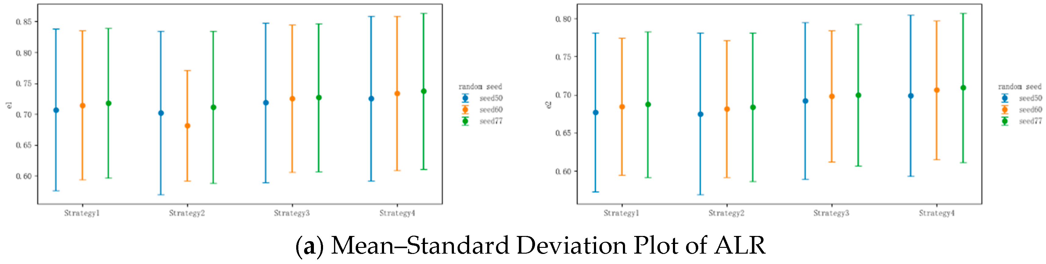
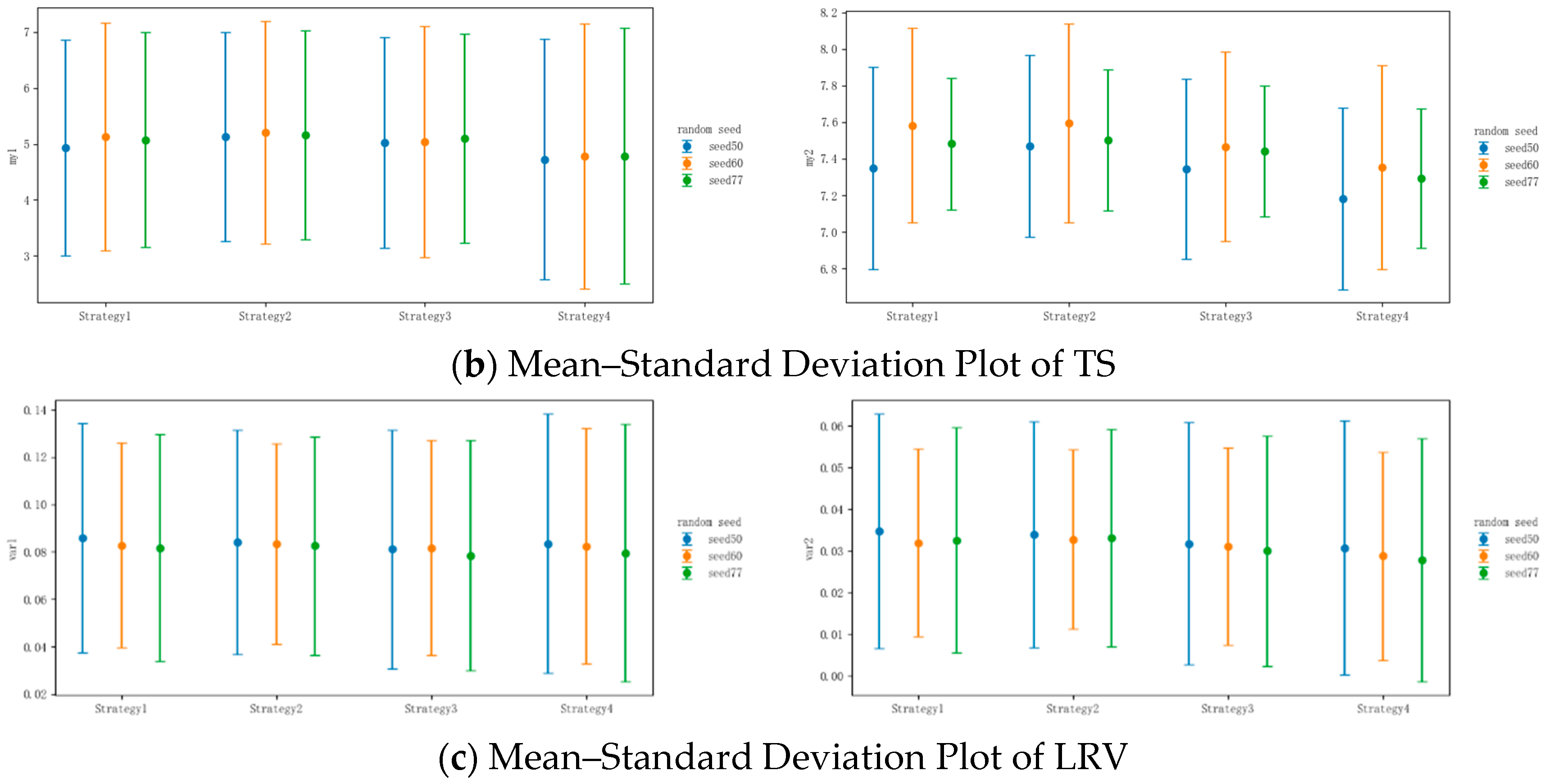
Figure 5 summarizes the mean values and standard deviations of ALR, TS, and LRV under multiple random seed conditions. The results show that all guidance strategies substantially reduce fluctuations compared with natural dispersion, while different strategies exhibit different trade-offs across efficiency, visitor experience, and stability.

The joint analysis of mean and standard deviation shows that the mean–standard deviation plots reveal overall performance improvements under the visitor guidance strategies while also highlighting differences in stability characteristics among strategies. These findings are consistent with the previously discussed temporal evolution analysis and before–after comparisons, and provide statistical support for the robustness of the strategies within the simulated peak-period scenarios.

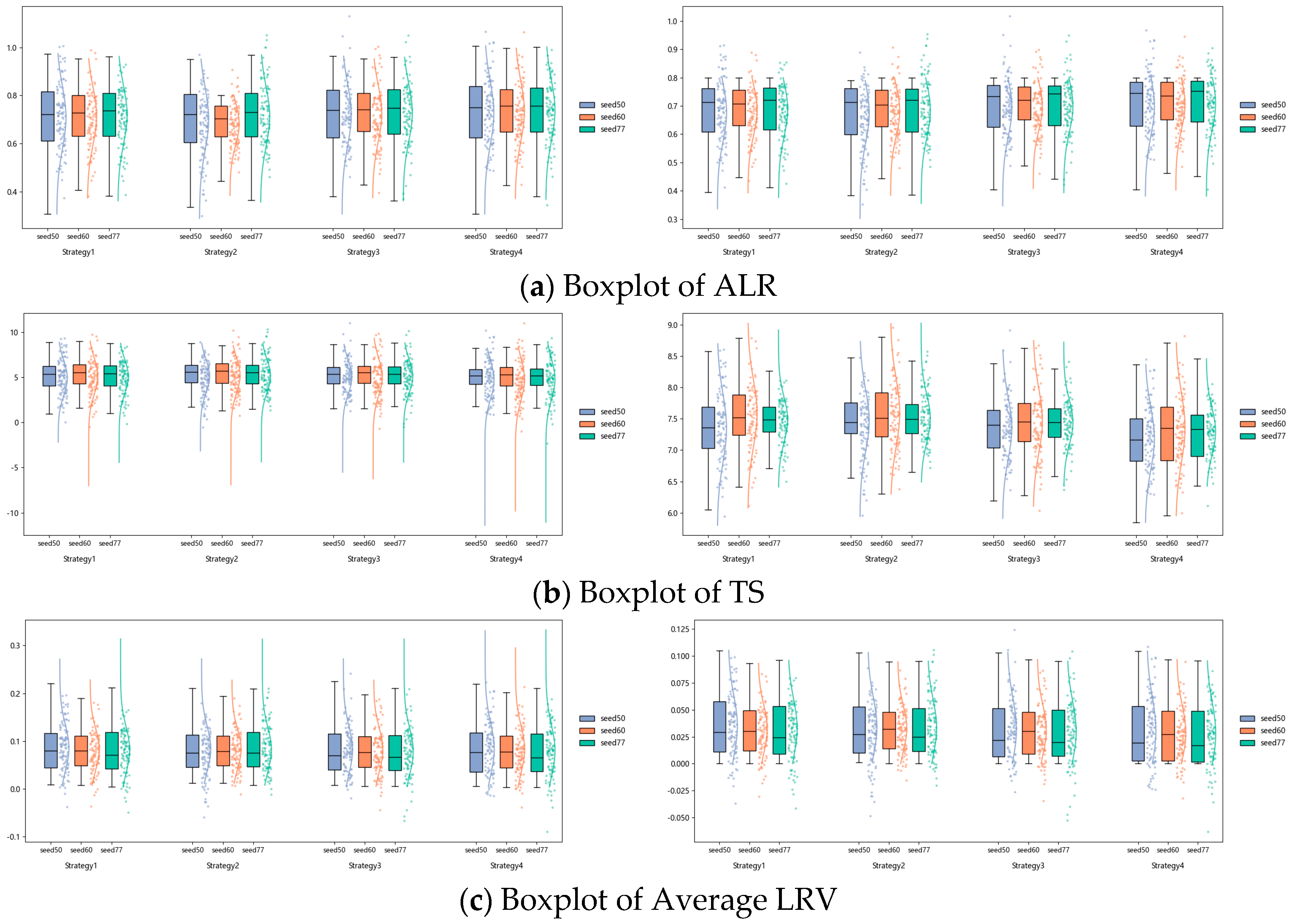
To further depict the distributional characteristics of evaluation indicators across time and under stochastic disturbances for different visitor guidance strategies, box plots are employed to statistically describe the indicator series, as shown in Figure A3.

Figure A3 further confirms the conclusions drawn from the mean–standard deviation analysis. Compared with natural dispersion, all guidance strategies shift the distributions of ALR and LRV downward, raise TS, and reduce overall dispersion, indicating improved load control, visitor experience, and operational stability under stochastic disturbances.

Overall, the boxplot analysis complements and corroborates the conclusions drawn from the mean–standard deviation analysis and the temporal evolution analysis. From a distributional perspective, these results indicate that the proposed tourist guidance strategies tend to improve load control, visitor experience, and operational stability simultaneously during peak periods within the simulation setting.

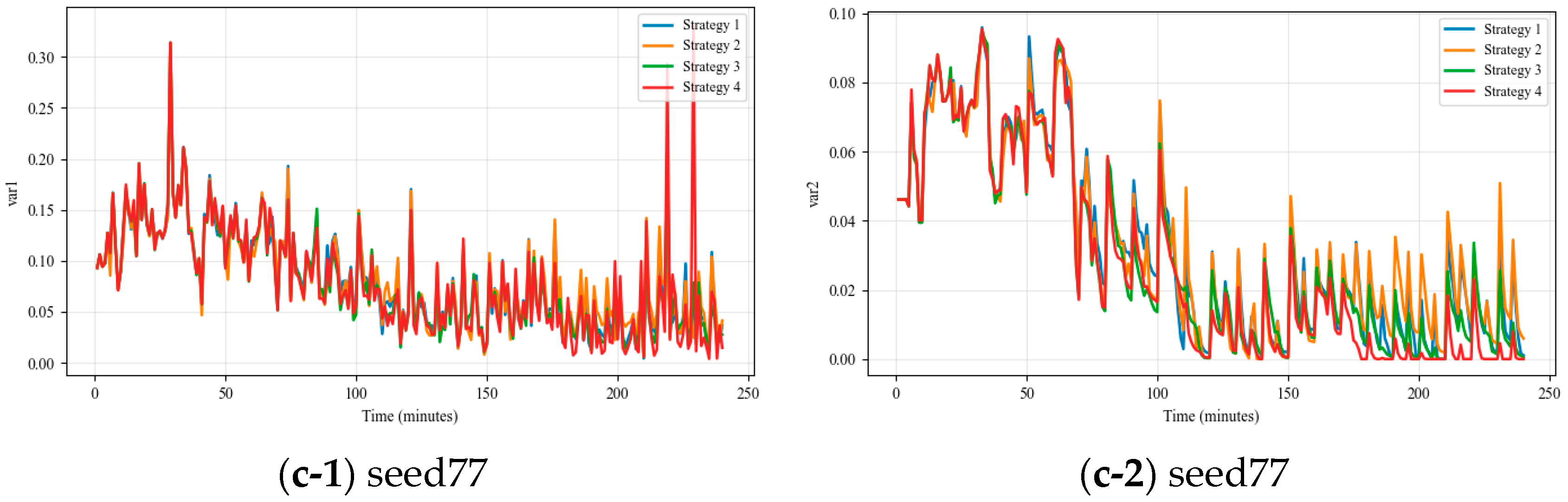
5.5. Dynamic Regulation Process Analysis at the Minute Scale

To further reveal the underlying mechanisms of the tourist guidance strategies, this section conducts a dynamic analysis of the scenic area’s operational state before and after the implementation of guidance strategies at a minute-level temporal resolution.

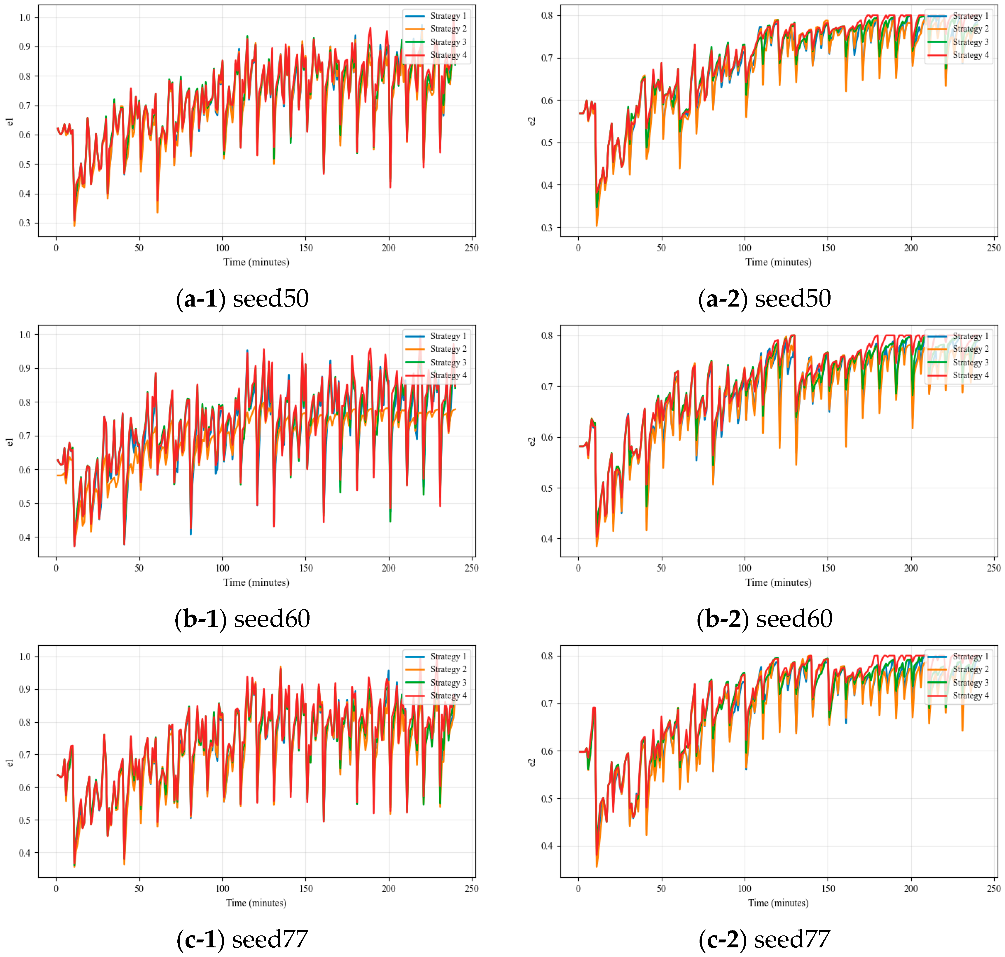
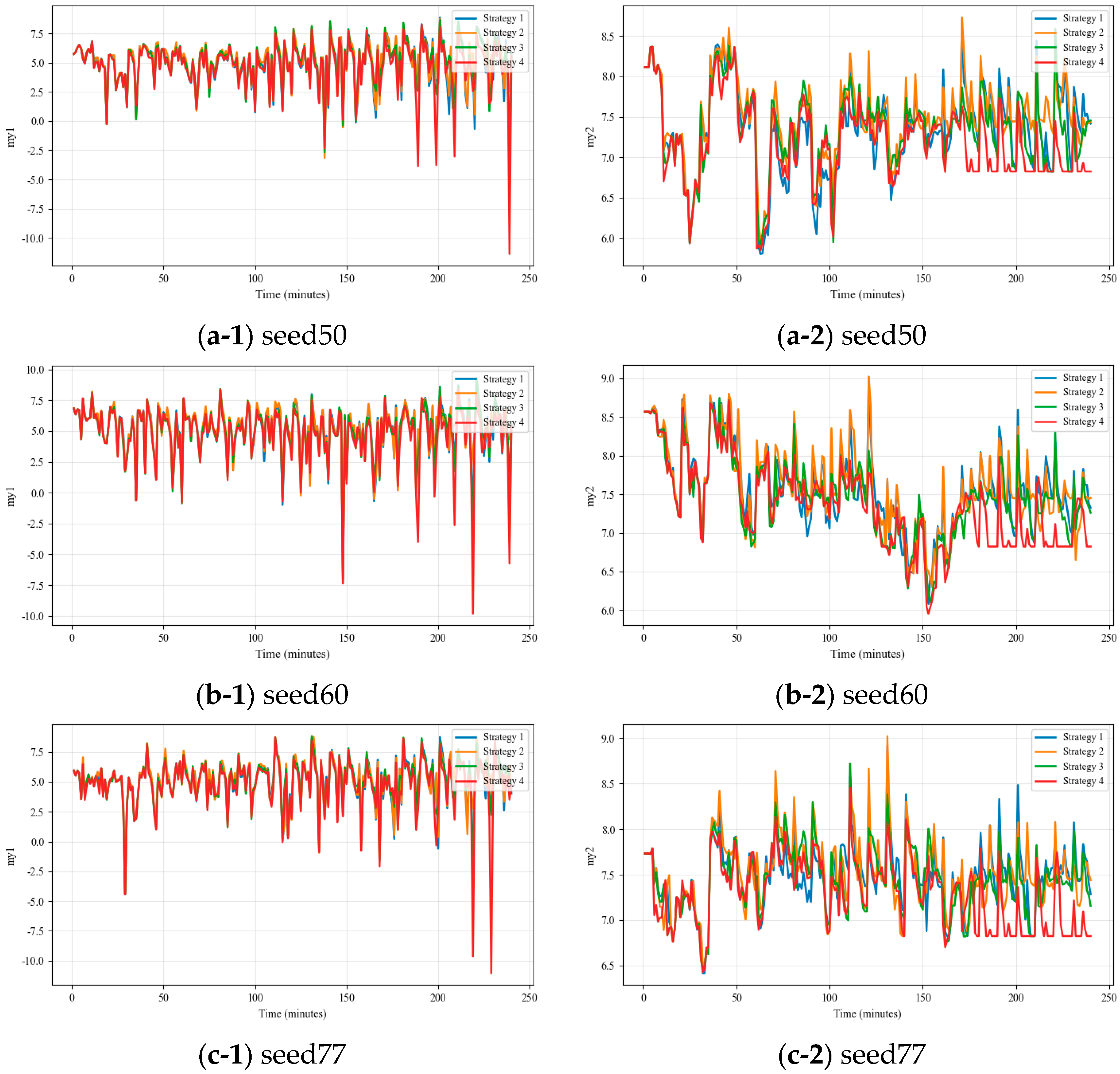
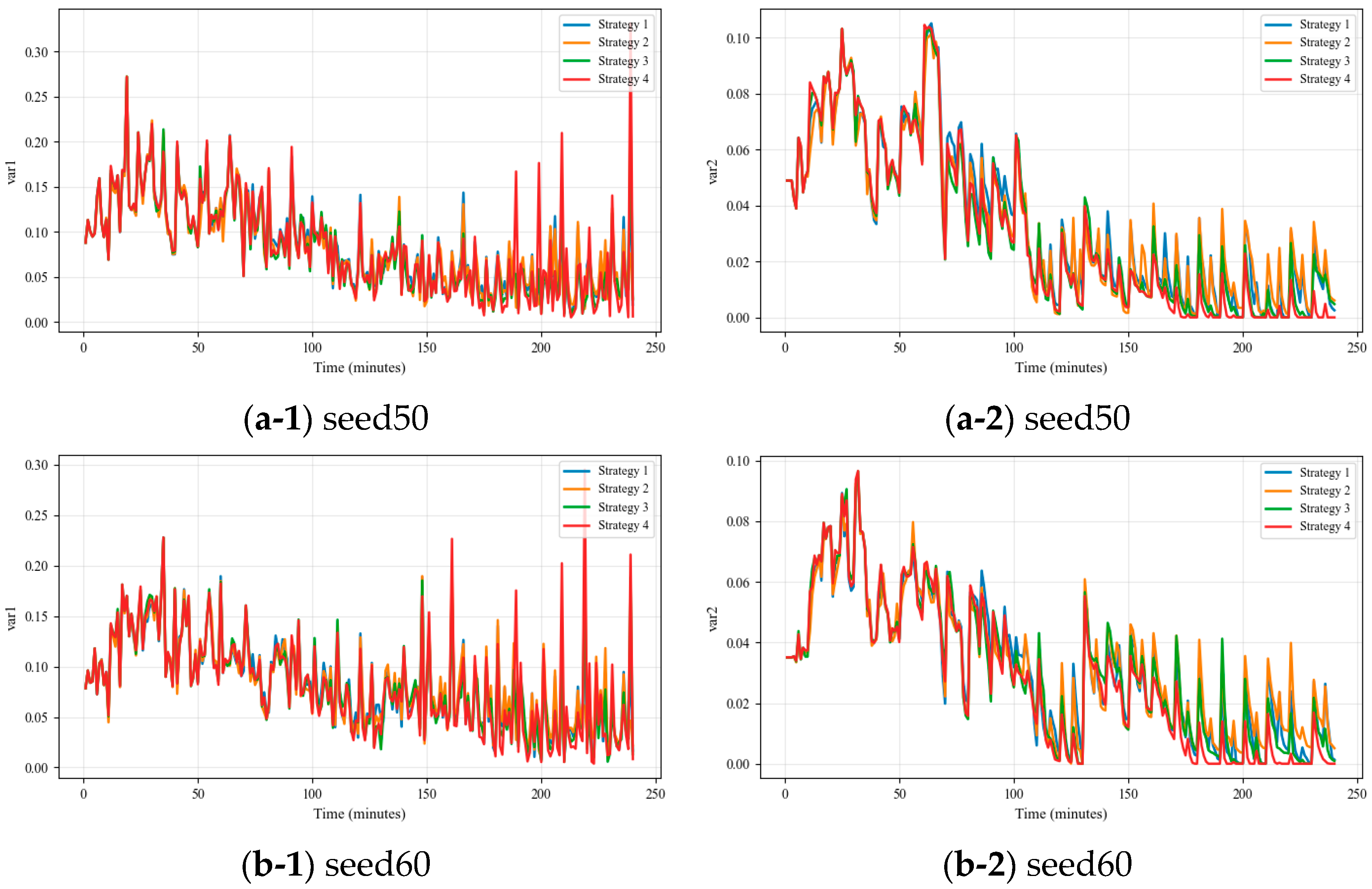
Figure 6, Figure A4 and Figure A5 show that under natural dispersion the system experiences persistent load accumulation, unstable satisfaction, and uneven spatial distribution. After applying guidance strategies, ALR decreases, TS improves, and LRV declines substantially across different random seeds, indicating that the strategies can suppress congestion propagation and stabilize system operation at the minute scale.

Overall, the dynamic results show that continuous minute-level intervention can suppress load accumulation, stabilize visitor experience, and improve spatial load distribution during peak periods. These conclusions corroborate the previous mean–standard deviation and boxplot analyses, providing consistent simulation-based evidence for the effectiveness of the tourist guidance strategies.

5.6. Joint Analysis of TS and ALR

5.6.1. Characteristics of the TS-ALR Relationship

Based on the preceding indicator analysis, it is necessary to further examine whether the relationship between TS and scenic area load remains stable under different random conditions. Considering that the goal of tourist guidance is not merely to reduce overall visitor numbers but to achieve a reasonable balance between visitor experience and spatial capacity under safety constraints, and that TS exhibits a significant nonlinear response to load, relying solely on static pre- and post-guidance comparisons cannot fully reveal the underlying mechanism. To address this, this study constructs the relationship curve between TS and the scenic area’s ALR. Under unchanged guidance strategies, different random seeds (seed50, seed60, seed77) are introduced for comparison to assess the consistency of this relationship under stochastic disturbances, thereby evaluating the robustness and reliability of different tourist guidance strategies in balancing multiple objectives.

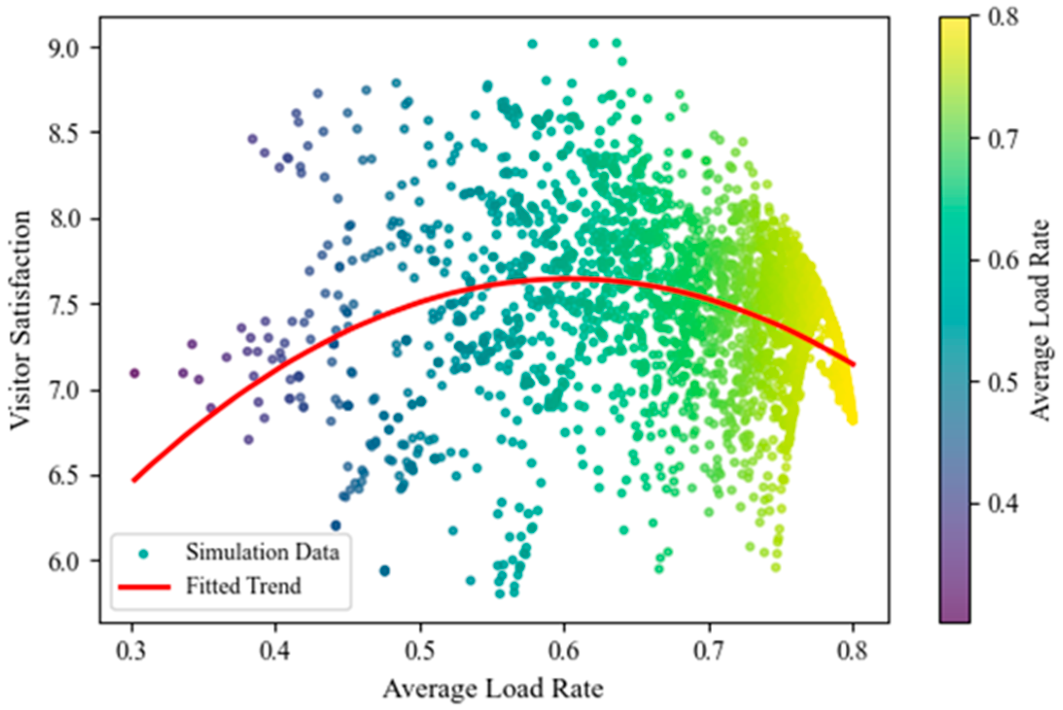
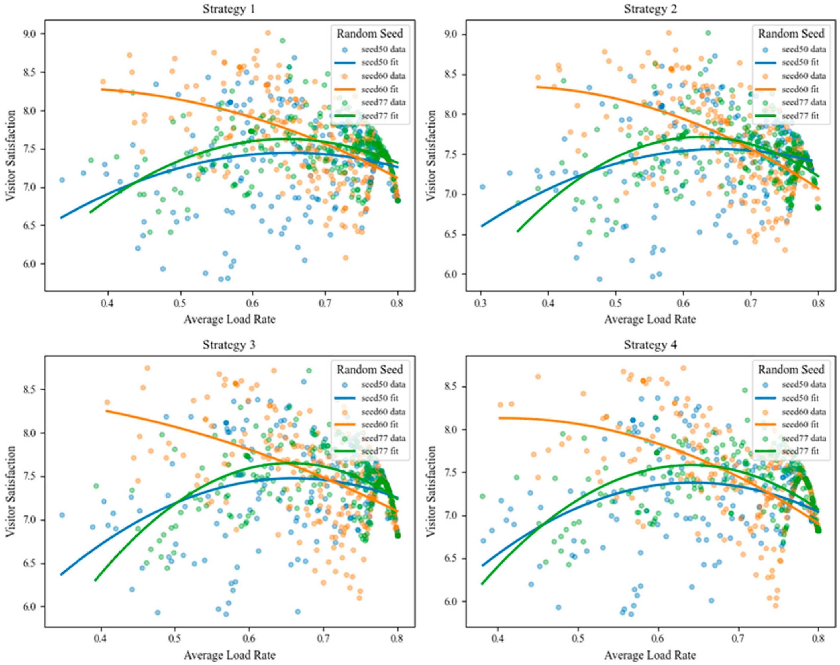
Figure 7 illustrates the relationship between TS and the ALR of the scenic area, derived from simulation data. In the figure, scatter points represent observed TS-ALR values obtained under different tourist guidance strategies, random seeds, and time scales; the fitted curve reflects the overall trend. It can be seen that the relationship exhibits a clear inverted U-shape, indicating that TS reaches its maximum at moderate load levels and decreases under both low and high load conditions.

The above analysis characterizes the relationship between TS and the ALR at a global level, revealing the generally observed inverted U-shaped pattern. However, since tourist arrivals and attraction choices are stochastic, this relationship may be influenced by random disturbances. To further examine the stability and robustness of the TS–ALR relationship under different random conditions, this study keeps the tourist guidance strategy unchanged while introducing different random seeds (seed50, seed60, seed77) to construct the TS–ALR curves and compare their differences.

Figure A6 presents the curves for TS versus ALR under various guidance strategies and random seed conditions. It can be observed that, for the same guidance strategy, the curves corresponding to different random seeds (seed50, seed60, seed77) generally maintain the inverted U-shaped pattern, indicating that this relationship is not dependent on a specific random disturbance. Although there are minor local differences between curves across seeds, the peak positions and overall trends are largely consistent, demonstrating that the model is robust in capturing how TS varies with load. Additionally, variations in curve shape and optimal load ranges across guidance strategies reflect the impact of different flow management approaches on visitor experience and load regulation.

Under certain random seeds (e.g., seed60), the TS–ALR curve does not show a fully symmetric inverted-U shape and instead appears closer to a monotonic decline over the observed load range. This variation mainly reflects the specific stochastic arrival and spatial flow pattern in that simulation run, rather than invalidating the overall nonlinear relationship between satisfaction and load.

5.6.2. Robustness Analysis Under Different Random Seeds

To quantitatively evaluate the robustness of the TS–ALR relationship, three indicators are introduced: optimal load rate deviation, optimal satisfaction fluctuation, and curve consistency. These metrics are used to assess the stability of the optimal operating range, the sensitivity of peak satisfaction, and the overall consistency of the TS–ALR relationship across random seeds.

Through this multi-metric robustness analysis, the reliability of different tourist guidance strategies in balancing multiple objectives can be quantitatively assessed, providing a solid foundation for subsequent strategy comparisons and effectiveness evaluations.

Table 8. Robustness Test Indicator Results.

Guidance Strategy	$\mathbf{Mean} \mathbf{Optimal} \mathbf{Load} \mathbf{Rate} {\overline{\mathit{L}}}_{\mathit{s}}^{*}$	$\mathbf{Optimal} \mathbf{Load} \mathbf{Rate} \mathbf{Deviation} {\mathit{D}}_{\mathit{\rho }}$	$\mathbf{Mean} \mathbf{Optimal} \mathbf{Satisfaction} {\overline{\mathit{S}}}_{\mathit{s}}^{*}$	$\mathbf{Optimal} \mathbf{Satisfaction} \mathbf{Fluctuation} {\mathit{D}}_{\mathit{S}}$	$\mathbf{Curve} \mathbf{Consistency} \mathbf{Index} {\mathit{D}}_{\mathit{C}}$
Strategy 1	0.5428	0.1504	7.7884	0.3650	0.9462
Strategy 2	0.5399	0.14161	7.8741	0.3413	1.0689
Strategy 3	0.4864	0.2418	7.8656	0.4341	2.1892
Strategy 4	0.5642	0.1110	7.6973	0.3169	1.6223

presents the robustness test results of different visitor guidance strategies under multiple random seed conditions. From the perspective of Optimal Load Rate Deviation, all strategies exhibit some fluctuation in the optimal load rate position under random disturbances, but the amplitude differs noticeably. Strategy 4 has the smallest deviation, indicating that its optimal load range is most concentrated across different random realizations and is less sensitive to random factors. Strategies 1 and 2 follow, showing relatively similar stability levels. In contrast, Strategy 3 exhibits a significantly larger deviation, indicating that its optimal load rate is more affected by random disturbances.

Regarding the Optimal Satisfaction Fluctuation indicator, the peak TS under all strategies remains at a similar level, though the fluctuation extent varies. Strategy 4 has the lowest fluctuation, showing that it can maintain a stable satisfaction peak under different random seeds. Strategies 1 and 2 show moderate fluctuations, while Strategy 3 has the highest value, indicating greater sensitivity of peak satisfaction to random factors and relatively weaker stability.

Further examining the Curve Consistency Index of the TS–ALR relationship reveals noticeable differences in the overall structural stability among strategies. Strategies 1 and 2 have relatively small indices, indicating that satisfaction curves under different random seeds are highly consistent within a unified load rate range, preserving the inverted-U shape and trend. Strategy 4′s index is higher than the first two but still acceptable, while Strategy 3 shows a significantly larger index, indicating more substantial differences in the overall curve shape across random seeds and weaker structural consistency.

Overall, the three robustness indicators suggest that the robustness of visitor guidance strategies under random disturbances is not uniform. Strategies 1 and 2 perform relatively balanced in terms of optimal range stability and structural consistency; Strategy 4 shows advantages in the stability of both optimal load and peak satisfaction, while Strategy 3, despite comparable average satisfaction, is more sensitive to random disturbances.

These results indicate that the goal of visitor guidance is not merely to minimize load levels but to achieve a reasonable balance between visitor experience and spatial carrying capacity under safety constraints. The optimal load ranges vary among strategies, reflecting different mechanisms of guidance in regulating path choice and load distribution.

6. Discussion

6.1. Main Findings and Mechanisms

It is first necessary to clarify the methodological rationale for employing TPN in this study. Although ABM is widely used in tourism and crowd simulations to represent heterogeneous visitor behavior, the objective of this study is different. Rather than reproducing individual-level behavior in detail, the model aims to analyze congestion propagation and regulation mechanisms at the system level within a scenic-area network. TPN provides a formal framework for representing concurrent processes, capacity constraints, and temporal dependencies among attractions and travel paths. Compared with ABM approaches, the TPN model explicitly captures flow transitions and resource limitations, allowing a clear representation of system states and load propagation. In addition, its relatively compact structure facilitates systematic comparison of multiple guidance strategies without requiring detailed behavioral parameters. In this sense, the TPN-based model complements rather than replaces behavior-oriented simulation approaches.

Minute-level simulations based on the network topology of Huangshan Scenic Area and peak-period arrival patterns indicate that guidance mechanisms can improve system operation without reducing the total number of visitors. The improvements arise mainly from the reorganization of the temporal–spatial distribution of visitors rather than from limiting visitor inflow.

Under the simulated peak-period scenario, the proposed guidance strategies substantially improve system performance compared with natural dispersal. Specifically, the average load rate was reduced by approximately 74%, and the spatial load distribution showed strong convergence. Visitor satisfaction shifted from extremely negative levels under natural dispersal to a stable positive range. These results suggest that severe congestion during peak periods is not inevitable; rather, effective mitigation depends on whether structured and continuous interventions can interrupt the positive feedback loop of “hotspot accumulation → overload propagation → fluctuation amplification.”

From a mechanistic perspective, the model reveals strong temporal and path dependency in visitor movement. Under natural dispersal, the interaction between stochastic arrivals, visitor preferences, and path topology can produce absorption effects at a small number of critical nodes, leading to persistent overload across consecutive time steps. The guidance mechanism intervenes dynamically at each time step by redistributing visitors across feasible downstream attractions, thereby mitigating hotspot accumulation and limiting downstream congestion propagation. In this way, the system is shifted from highly fluctuating states toward a more stable and controllable operating regime, reflecting the classical management principle of “peak shaving and valley filling.”

Although all four guidance strategies produce positive regulatory effects, their mechanisms differ in terms of information scope and regulatory focus. Strategies based on balanced distribution or attraction weights rely mainly on structural information or visitor preference tendencies and therefore perform well in reducing initial load accumulation. In contrast, strategies based on attraction or path load incorporate system-state information and show stronger capability in alleviating localized congestion and improving spatial load balance. These findings suggest that the effectiveness of a guidance strategy depends not only on the quantity of information used but also on the alignment between information type and management objectives.

The simulation results also reveal a consistent inverted-U relationship between tourism satisfaction and scenic area load across different strategies and random conditions. This finding quantitatively supports a well-recognized principle in scenic-area management: both excessively low and excessively high visitor loads may negatively affect visitor experience, while an intermediate load range can balance safety and recreational atmosphere. Traditional management approaches often emphasize reducing load levels, potentially overlooking the experience loss caused by excessive dispersion. In contrast, the proposed dynamic guidance approach focuses on maintaining system operation within a relatively optimal load range under safety constraints, thereby achieving a balance between visitor experience and spatial carrying capacity.

Simulations conducted under multiple random seeds further indicate that the main conclusions remain consistent under different stochastic disturbances, suggesting a certain degree of robustness to uncertainties in visitor arrivals and behavioral variability.

Finally, the proposed guidance strategies rely mainly on locally observable system-state information and simple decision rules rather than global optimization or computationally intensive procedures, which enhances their potential applicability in real-world management scenarios. From an operational perspective, the model should therefore be viewed as a decision-support framework rather than a standalone management system. In practice, conventional interventions—such as improved signage systems, timed ticketing policies, and staff deployment at congestion-prone locations—remain essential components of visitor flow regulation. The guidance strategies analyzed in this study can complement these measures by helping managers identify congestion hotspots and critical time periods where targeted interventions may be most effective.

6.2. Research Limitations and Future Work

Although this study systematically evaluated the effectiveness of visitor guidance strategies during peak periods from the perspectives of temporal evolution, statistical distribution, and random disturbances, certain limitations remain.

First, the simulation model simplifies visitor behavior to some extent—for example, assuming uniform walking speeds and fixed visiting durations—without fully considering individual heterogeneity. In addition, the model assumes that tourists who receive guidance follow the recommended routes, while in real-world scenarios visitor compliance with guidance may vary and some tourists may even respond contrarily. Second, this study focuses on aggregation and load balancing at the attraction level but does not explicitly model road capacities or traffic conflicts between attractions, which may have non-negligible effects in real-world scenarios. Finally, the case study is based on an abstracted topology of Huangshan Scenic Area, and the generalizability of the findings to other types of scenic areas requires further empirical validation. Future research can be expanded in several directions: (1) Incorporate more detailed visitor behavior modeling, including heterogeneous preferences, adaptive path selection, and probabilistic compliance with guidance. (2) Integrate road capacities, traffic conflicts, and safety constraints into the modeling approach to better capture extreme congestion scenarios. (3) Combine real-time sensing data and smart devices to explore the online application of visitor guidance strategies in real scenic environments and enable feedback-based optimization mechanisms. In addition, the current study relies primarily on simulation experiments for evaluation. Although key parameters were calibrated using available planning information and historical visitor statistics, further validation using real-time visitor monitoring data and operational records is necessary to fully assess the practical effectiveness of the proposed framework in real scenic area management.

7. Conclusions

This study addresses the problem of visitor congestion and load imbalance in scenic areas during peak tourism periods by developing a dynamic visitor guidance modeling and analysis approach based on TPNs. Using Huangshan Scenic Area as a case study, the simulation experiments systematically evaluated the operational effects of different visitor guidance strategies under peak-period conditions. The focus is not on reducing the total number of visitors but on optimizing their spatial distribution within the scenic area through dynamic guidance, thereby enhancing operational efficiency, visitor experience, and system stability simultaneously.

Simulation results indicate that under natural dispersal conditions, the scenic area exhibits high load, high fluctuation, and low satisfaction during peak periods. When visitor guidance strategies are implemented in the simulation experiments, the ALR significantly decreases, TS rises from low values to a stable positive range, inter-attraction load distribution becomes more balanced, and system fluctuations are substantially reduced. Minute-level dynamic analysis further demonstrates that visitor guidance strategies continuously suppress load accumulation and regulate scenic operations in real time, effectively “shaving peaks and filling valleys”.

At the strategic level, all guidance strategies based on different information scopes can play a positive role during peak periods. The differences among strategies mainly lie in the trade-offs between load control, experience enhancement, and spatial balance, rather than in overall effectiveness. Joint analysis reveals a stable inverted-U relationship between TS and scenic load, suggesting that the core objective of scenic management should be to maintain operations within a reasonable load range under safety constraints, rather than merely pursuing minimal load. Robustness tests under multiple random conditions further support that the findings are insensitive to random disturbances, enhancing the reliability of the results.

In summary, the proposed dynamic visitor guidance approach demonstrates novelty in modeling methodology, strategy design, and effect evaluation. It provides a quantitative analytical tool that can support decision-making in visitor management during peak periods. The findings offer theoretical guidance and methodological reference for implementing dynamic visitor guidance under limited information and response capabilities. Future studies may further enhance the model’s applicability to complex real-world scenarios by incorporating visitor behavioral heterogeneity, road capacity constraints, and real-time sensing data.