Article

From Hours to Milliseconds: Dual-Horizon Fault Prediction for Dynamic Wireless EV Charging via Digital Twin Integrated Deep Learning

Electrical Engineering Department, Yanbu Industrial College, Yanbu 41912, Saudi Arabia
*
Author to whom correspondence should be addressed.
Smart Cities 2026, 9(3), 43; https://doi.org/10.3390/smartcities9030043
Submission received: 12 January 2026 / Revised: 17 February 2026 / Accepted: 22 February 2026 / Published: 26 February 2026

Highlights

What are the main findings?
  • DNN achieves 97.85% accuracy for 8-class DWPT fault detection with statistical significance (p < 0.001) compared to baseline methods (SVM, Random Forest, LSTM).
  • Digital twin infrastructure enables dual-horizon prediction: long-term forecasting (24–72 h) for incipient faults and real-time detection under 50 ms for critical grid protection.
  • Multi-station sensor fusion with 36 features improves detection accuracy by 6.38% compared to single-station configurations.
What are the implications of the main findings?
  • Reliable AI-based fault detection enables safe deployment of DWPT as smart city EV charging infrastructure.
  • Real-time protection capability (4.2 ms inference latency) meets critical 10–50 ms grid protection timing requirements.
  • Practical parameter acquisition methodology enables real-world deployment of the proposed framework.

Abstract

Dynamic Wireless Power Transfer (DWPT) is emerging as critical smart city infrastructure for sustainable urban mobility, enabling electric vehicle charging while driving. However, DWPT introduces complex fault scenarios requiring intelligent monitoring. Existing fault diagnosis approaches for wireless power transfer systems face three key complexities: (1) they are limited to static charging with only 2–4 fault categories, failing to address the time-varying coupling dynamics and segmented coil handover transients inherent in dynamic charging; (2) they lack integration with the host distribution grid, ignoring grid-side disturbances that propagate to charging stations; and (3) they offer only reactive detection without predictive capability for incipient fault management. This paper presents a deep neural network (DNN)-based fault diagnosis framework utilizing multi-station sensor fusion for DWPT systems integrated with the IEEE 13-bus distribution network to address these limitations. The system monitors 36 sensor features across three charging stations, employing feature-level concatenation with station-specific normalization for multi-station fusion, achieving 97.85% classification accuracy across eight fault types. Unlike static charging, the framework explicitly models time-varying coupling dynamics due to vehicle motion, including segmented coil handover effects. A digital twin provides dual-horizon prediction: long-term forecasting (24–72 h) for incipient faults and real-time detection under 50 ms for critical protection, with fault probability outputs and ranked fault lists enabling actionable maintenance decisions. The DNN outperforms SVM (92.45%), Random Forest (94.82%), and LSTM (96.54%) with statistical significance ( p < 0.001 ), while maintaining model inference latency of 4.2 ms, suitable for edge deployment. Circuit-based analysis provides analytical justification for fault signatures, and practical parameter acquisition methods enable real-world implementation. Five case studies validate robustness across highway, urban, and grid disturbance scenarios with detection accuracies exceeding 95%.

1. Introduction

The global transition toward sustainable transportation has accelerated the adoption of electric vehicles (EVs), with global EV sales exceeding 17 million units in 2024 (over 20% market share) and projected to surpass 20 million units in 2025, representing more than one in four new cars sold worldwide according to the International Energy Agency (IEA) [1]. However, charging infrastructure limitations, including long charging times and range anxiety, remain significant barriers to widespread EV adoption. Dynamic Wireless Power Transfer (DWPT) technology offers a promising solution by enabling EVs to charge while driving, potentially eliminating the need for frequent stops and reducing battery capacity requirements [2,3]. Recent comprehensive reviews have highlighted the critical role of power electronic converters in enabling efficient EV charging across various topologies [4].
DWPT systems operate on the principle of magnetic resonance coupling, transferring power from transmitter coils embedded in the roadway to receiver coils mounted on vehicles [5,6]. While this technology presents numerous advantages, including convenience and extended driving range, it also introduces complex fault scenarios that can significantly impact system performance and safety. Faults in DWPT systems can arise from various sources, including coil damage, foreign object intrusion, severe misalignment, power electronics failures, and thermal issues [7,8]. As highlighted in recent smart grid fault classification studies, understanding diverse fault types, including incipient, abrupt, and intermittent faults, and their impacts is essential for ensuring system stability [9].
Traditional fault detection methods in power systems rely on threshold-based approaches or physics-based models, which may not effectively capture the complex, nonlinear dynamics of DWPT systems [10]. The advent of artificial intelligence (AI) and machine learning (ML) techniques has opened new possibilities for intelligent fault detection and diagnosis [11,12]. Deep learning models, in particular, have demonstrated remarkable capabilities in pattern recognition and classification tasks, making them well-suited for analyzing the high-dimensional, time-varying data generated by DWPT sensor systems [13]. Neural network approaches have proven effective in various power system applications, including solar PV power estimation and forecasting [14].
Digital twin technology has emerged as a powerful paradigm for creating virtual replicas of physical systems, enabling real-time monitoring, simulation, and predictive analytics [15,16]. The integration of digital twins with AI-based fault detection offers unprecedented capabilities for predictive maintenance and system optimization [17,18]. However, the application of digital twin-enabled fault diagnosis to grid-integrated DWPT systems remains unexplored. The growing penetration of distributed energy resources and EVs in modern power systems necessitates flexible demand-side management strategies to maintain grid stability [19]. Comprehensive reviews of microgrid protection challenges have demonstrated the importance of systematic approaches to fault management in power systems with renewable energy resources [20].
This paper presents an AI-driven fault management and diagnosis framework with digital twin integration for DWPT systems on the IEEE 13-bus distribution network. To clarify the terminology used throughout this paper: “DWPT” refers specifically to dynamic (in-motion) wireless power transfer, while “WPT” denotes the broader wireless power transfer field including static charging. “Fault detection” refers to the binary identification of abnormal operation, while “fault diagnosis” encompasses detection plus classification of the specific fault type and its root cause. “Inference latency” refers to the DNN model computation time alone (4.2 ms), whereas “end-to-end system latency” includes sensor acquisition, preprocessing, inference, and protection actuation (<50 ms total). The main contributions of this work include:
1.
First integration of AI-based fault detection with digital twin technology for DWPT systems on the IEEE 13-bus distribution network, enabling predictive and grid-aware fault diagnosis through multi-station sensor fusion;
2.
Explicit modeling of dynamic charging characteristics including time-varying coupling coefficients, segmented coil handover transitions, and speed-dependent fault signatures—differentiating this work from static WPT fault detection approaches;
3.
Comprehensive 8-class fault taxonomy covering coil faults, power electronics failures, foreign object detection, misalignment, and thermal issues—significantly more comprehensive than existing 2–4 class approaches;
4.
Circuit-based analytical derivations explaining the physical mechanisms behind each fault signature, supported by equivalent circuit analysis for the series–series (SS) compensation topology;
5.
Digital twin framework with adaptive state synchronization enabling long-term prediction of incipient faults (24–72 h) and short-term early warning for impending failures (30–60 min);
6.
Practical parameter acquisition methodology detailing how each of the 36 sensor features can be measured or estimated in real-world deployments;
7.
Comprehensive benchmarking against six alternative ML/DL methods achieving superior classification accuracy (97.85% ± 0.42%, p < 0.001 vs. baselines), with real-time detection capability under 50 ms latency.
The remainder of this paper is organized as follows: Section 2 reviews the related work. Section 3 presents the materials and methods including system modeling, fault types, and the proposed AI framework. Section 4 presents results and case studies. Section 5 provides discussion. Section 6 concludes the paper.

2. Related Work

2.1. DWPT Technology and Grid Integration

Research on DWPT integration with distribution networks has primarily focused on grid impact analysis and control strategies. Early foundational work by Covic and Boys [5] established the theoretical basis for inductive power transfer, while subsequent studies extended these principles to dynamic applications. Hui et al. [21] provided a critical review of the mid-range wireless power transfer progress, analyzing the fundamental operating principles under maximum power transfer and maximum energy efficiency paradigms, which underpin the coupling models adopted in this work. Shi et al. [22] proposed an integrated solution combining electric vehicle detection and foreign object detection for dynamic inductive power transfer applications for grid interface. Building on this grid-centric perspective, Mi et al. [3] reviewed modern advances in wireless power transfer systems for roadway-powered EVs, highlighting the challenges of grid integration and power quality. Lukic and Pantic [23] compared static and dynamic inductive wireless charging approaches, emphasizing the infrastructure requirements.
From a power electronics perspective, Onar et al. [24] demonstrated a novel wireless power transfer system for in-motion EV charging with grid interface considerations. Ali et al. [4] provided a comprehensive review of charging topologies and power electronic converter solutions for EVs, covering AC and DC charging methods, wireless power transfer, and vehicle-to-grid (V2G) technologies. Jo and Kim [25] recently presented a simplified integration of bidirectional on-board charger and WPT charging systems with reconfiguring topology for electric vehicles, demonstrating the ongoing convergence of charging system architectures that motivates comprehensive fault monitoring across interconnected power electronic stages. These studies collectively establish the foundation for understanding DWPT–grid interactions; however, none address comprehensive sensor-based fault detection that accounts for the unique dynamic characteristics of in-motion charging.

2.2. Fault Diagnosis for WPT Systems

Fault diagnosis methods for wireless power transfer systems have evolved significantly. Traditional approaches relied on threshold-based monitoring of electrical parameters, which proved insufficient for capturing the complex, nonlinear fault dynamics in resonant systems [10]. Zhang et al. [8] provided a comprehensive overview of foreign object detection technologies in wireless power transfer systems, categorizing detection methods for main circuit fault diagnosis. However, these methods are limited to stationary charging scenarios with typically 2–4 fault categories. This limitation motivates this paper’s extension to dynamic scenarios with a more comprehensive fault taxonomy.
Lu et al. [26] provided a comprehensive review of foreign object detection methods for wireless power transfer systems, covering detection methods for both metal objects and living objects that pose safety hazards in WPT applications. Tavakoli and Pantic [27] provided the analysis, design, and experimental demonstration of a 25 kW dynamic wireless charging system. Zhang et al. [8] reviewed foreign object detection methods for WPT. Krivohlava et al. [9] presented a comprehensive systematic literature review of fault types and failures in smart grid systems, surveying 30 different faults categorized into incipient, abrupt, and intermittent types. Their fault taxonomy and detection timing requirements of 10–50 ms directly inform this paper’s sensor framework design and real-time processing constraints.

2.3. Digital Twin Technology

Digital twin technology has gained significant attention for industrial applications. Tao et al. [15] presented the state of the art in digital twins for industry, outlining key technologies and applications. Grieves and Vickers [16] introduced the conceptual framework for digital twins in complex systems. Their five-dimensional model comprising the physical entity, the virtual entity, services, data, and connections provides the architectural foundation adopted in this paper’s framework. Qi et al. [17] surveyed enabling technologies and tools for digital twin implementation. Minerva et al. [18] provided a comprehensive survey on digital twins in the IoT context, covering technical features and architectural models.
In the power systems domain, Jafari et al. [28] presented a comprehensive review of digital twin technology in a smart grid, transportation system, and smart city applications. Heluany and Gkioulos [29] conducted a systematic literature review on digital twins for power generation and distribution, identifying five key components: physical entity, bidirectional communication, virtual entity, data management, and services. While these works establish digital twin principles for power systems, the work in this paper represents the first application specifically targeting DWPT fault diagnosis with grid integration.

2.4. Deep Learning for Fault Detection

The selection of deep learning over alternative machine learning approaches for fault detection warrants careful justification. LeCun et al. [12] provided a comprehensive overview of deep learning fundamentals, demonstrating that deep architectures excel at learning hierarchical feature representations from raw data. Goodfellow et al. [13] detailed neural network architectures suitable for pattern recognition. For fault detection specifically, DNNs offer three key advantages over traditional ML methods: (1) automatic feature extraction eliminating manual engineering, (2) superior performance on high-dimensional data, and (3) faster inference times compared to ensemble methods like Random Forest for real-time applications [30].
Hochreiter and Schmidhuber [31] introduced LSTM networks for sequence modeling, which have been applied to time series fault detection. However, while LSTMs capture temporal dependencies, their sequential processing limits parallelization and increases inference latency—a critical consideration for the sub-50 ms detection requirement in protection systems. Sharkawy et al. [14] demonstrated the effectiveness of different artificial neural network types (MLFFNN, RNN, NARX) for solar PV power estimation and forecasting, validating the applicability of neural networks in renewable energy systems and power quality applications. Recent advances include Thomas et al. [30], who proposed a CNN-based Transformer model achieving over 95% accuracy for fault detection in power system networks. Rizeakos et al. [32] developed deep learning-based applications for fault location identification and type classification in active distribution grids.

3. Materials and Methods

3.1. Dynamic Wireless Power Transfer System Model

The DWPT system model is based on the SAE J2954 WPT3 class specifications [2], operating at a resonant frequency of 85 kHz with a rated power of 11 kW. The system comprises a transmitter unit embedded in the roadway and a receiver unit mounted on the vehicle underside. Power is transferred through magnetic resonance coupling between the transmitter and receiver coils [33].
The mutual inductance M between the coils is given by
M = k L t x · L r x
where k is the coupling coefficient (typically 0.1–0.3 for DWPT) and L t x and L r x are the transmitter and receiver inductances (H), respectively.

3.1.1. Dynamic Coupling Model

Unlike static wireless charging systems, DWPT systems exhibit time-varying coupling characteristics due to vehicle motion. As the vehicle travels along the charging lane at velocity v, the coupling coefficient varies with the vehicle’s position x ( t ) = x 0 + v · t relative to the transmitter coil center. The instantaneous coupling coefficient is modeled as
k ( t ) = k 0 exp ( x ( t ) x c o i l ) 2 2 σ x 2 d 2 2 σ d 2
where k 0 is the peak coupling coefficient when perfectly aligned, x c o i l is the transmitter coil center position, d is the air gap distance, and σ x = 120 mm and σ d = 80 mm are characteristic decay constants derived from finite element analysis of the magnetic field distribution [33].
For a segmented transmitter coil array with coil spacing L c , the vehicle experiences periodic coupling variations as it passes over successive coils. The aggregate coupling from multiple coils is
k t o t a l ( t ) = i = 1 N c k i ( t ) = i = 1 N c k 0 exp ( x ( t ) i · L c ) 2 2 σ x 2
where N c is the number of active coils. This time-varying coupling introduces dynamic effects not present in static charging, including handover transients when transitioning between coils and speed-dependent power fluctuations.

3.1.2. System Efficiency Model

For the series–series (SS) compensation topology employed in this study, the maximum power transfer efficiency at optimal load matching is given by [33]
η m a x = k 2 Q t x Q r x 1 + 1 + k 2 Q t x Q r x 2 · η p e
where Q t x and Q r x are the quality factors of the transmitter and receiver coils, respectively, and η p e is the power electronics efficiency. Equation (4) is derived specifically for SS compensation; other topologies (SP, PS, PP) yield different efficiency expressions due to their distinct impedance transformation characteristics [6].
The system employs series–series (SS) compensation topology, where series capacitors are connected to both transmitter and receiver coils to achieve resonance at 85 kHz. The compensation capacitance C is calculated as
C = 1 ( 2 π f r ) 2 L
where f r is the resonant frequency and L is the coil inductance. This yields C = 17.6 nF for L = 200 μH at 85 kHz. Table 1 summarizes the key DWPT system parameters used in this study.

3.2. IEEE 13-Bus Distribution System

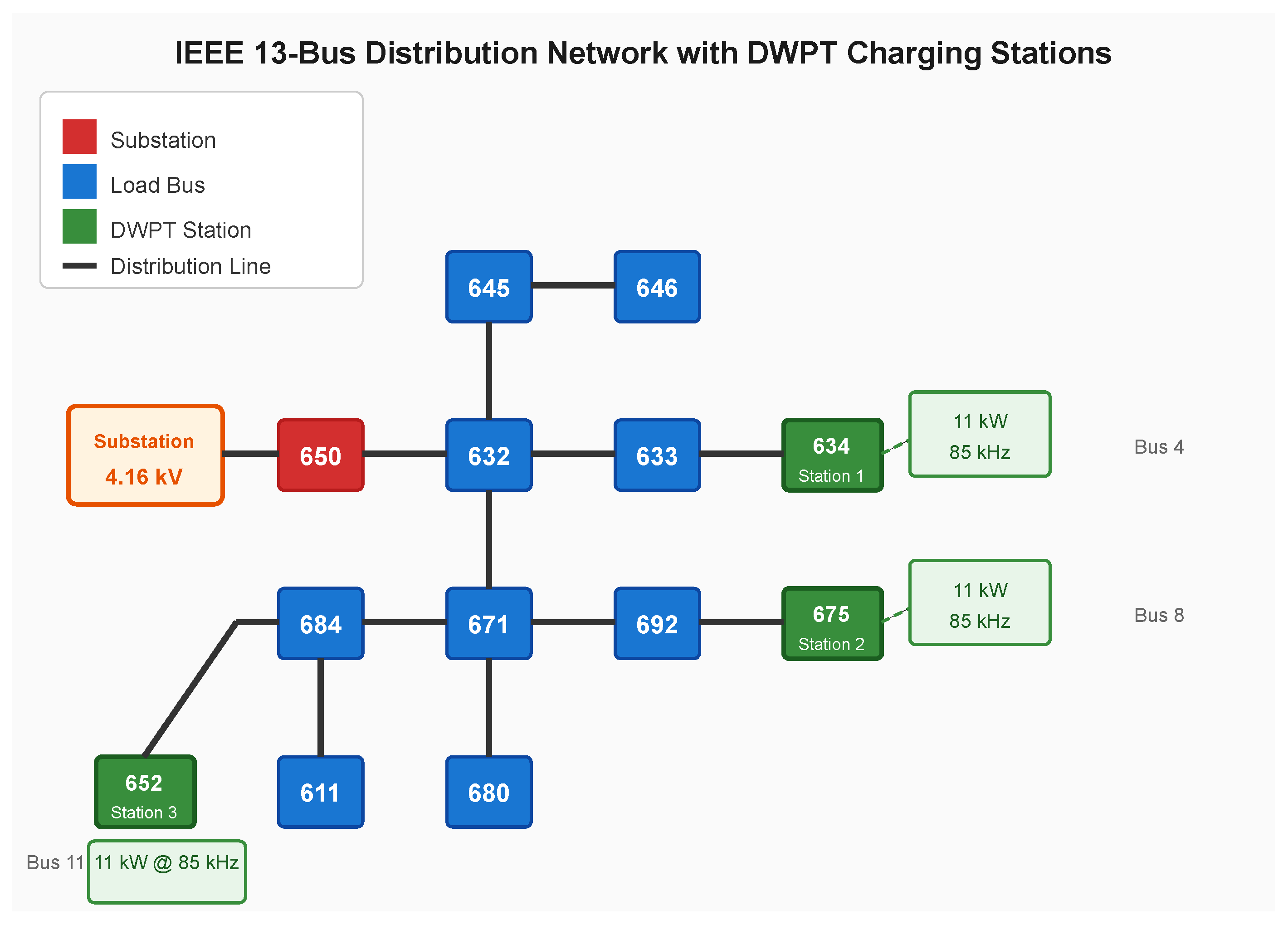
The IEEE 13-bus test feeder is a well established benchmark for distribution system analysis [34]. In this study, we integrate three DWPT charging stations at buses 4 (Node 634), 8 (Node 675), and 11 (Node 652). The system operates at 4.16 kV with a base power of 5 MVA. Each DWPT station can deliver up to 11 kW per charging lane. Figure 1 illustrates the IEEE 13-bus network topology with integrated DWPT stations.
The bus locations were strategically selected based on three criteria: (1) bus 4 (Node 634) is positioned near the sub-station Transformer, representing high traffic commercial areas with stable voltage profiles; (2) bus 8 (Node 675) is located at a network branch point with mixed residential/commercial loads, testing fault detection under variable loading conditions; and (3) bus 11 (Node 652) is at a feeder endpoint with single-phase laterals, representing challenging scenarios with potential voltage fluctuations.

3.3. Fault Types and Characteristics

Following the fault categorization framework established in the smart grid literature [9], this paper classifies DWPT faults into three categories: incipient faults (gradual degradation), abrupt faults (sudden failures), and intermittent faults (transient issues). The proposed system is designed to detect and classify eight distinct fault types:
  • Coil Open Circuit (COC): [Abrupt] Complete or partial break in the transmitter or receiver coil winding.
  • Coil Short Circuit (CSC): [Abrupt] Inter-turn short circuit causing excessive current and rapid temperature rise.
  • Capacitor Degradation (CD): [Incipient] Drift in compensation capacitor value due to aging or thermal stress.
  • Foreign Object Detection (FOD): [Intermittent] Metal objects in the charging zone causing eddy current losses.
  • Severe Misalignment (SM): [Intermittent] Excessive offset between transmitter and receiver coils ( k < 0.05 ).
  • Inverter Fault (IF): [Abrupt] Power electronics failure causing increased harmonic distortion.
  • Communication Fault (CF): [Intermittent] Control system communication issues causing erratic charging behavior.
  • Thermal Fault (TF): [Incipient] Overtemperature condition exceeding safe limits (>120 °C).

3.3.1. Dynamic Specific Fault Considerations

Beyond the eight fundamental fault types, DWPT systems exhibit unique fault modes not present in static charging:
Handover Fault (HF): During the transition between segmented transmitter coils, improper timing of coil activation/deactivation can cause power interruptions or transient overvoltages. The handover region spans approximately ± 0.3 L c around each coil boundary.
Speed-Induced Coupling Variation: At high vehicle speeds (>100 km/h), the rate of coupling change dk/dt increases, potentially causing control system instability if the tracking bandwidth is insufficient. The coupling rate of change is
d k d t = k 0 · v · ( x x c o i l ) σ x 2 exp ( x x c o i l ) 2 2 σ x 2
These dynamic effects are captured in the training dataset through speed parameterized simulations and are reflected in the speed feature (v) included in the sensor measurements.

3.3.2. Circuit-Based Fault Analysis

To provide analytical justification for the fault signatures in Table 2, this paper derives the expected parameter changes using the SS compensated equivalent circuit model. The primary and secondary circuit equations at resonance are [6]:
V t x = I t x ( R t x + j ω L t x + 1 j ω C t x ) + j ω M I r x = I t x R t x + j ω M I r x
0 = I r x ( R r x + R L + j ω L r x + 1 j ω C r x ) + j ω M I t x = I r x ( R r x + R L ) + j ω M I t x
From these equations, this paper derives fault specific behaviors:
Coil Open Circuit (COC): When the transmitter coil develops an open circuit, I t x 0 while the source attempts to maintain voltage, causing V t x to spike toward the open circuit source voltage. This distinguishes COC from a non activated coil, which shows both V t x = 0 and I t x = 0 .
Coil Short Circuit (CSC): An inter-turn short reduces effective inductance L t x < L t x , detuning the resonance. The reduced impedance causes I t x to increase dramatically. However, the power transferred to the receiver decreases because the shorted turns dissipate energy locally: P r x = I r x 2 R L decreases as the magnetic coupling efficiency degrades.
Capacitor Degradation (CD): When capacitance drifts from nominal ( C C ), the circuit detunes from resonance. The impedance becomes
Z t x = R t x + j ω L t x 1 ω C
For C < C (typical aging), the reactive component becomes inductive, increasing | Z t x | and thus V t x for constant current drive, or reducing I t x for constant voltage drive.
Severe Misalignment (SM): Reduced coupling ( k ) increases the reflected impedance seen by the primary: Z r e f = ω 2 M 2 / Z r x . With lower M, the primary current I t x must increase to maintain power transfer.
Table 2 presents the expected sensor feature changes for each fault type, derived from the circuit analysis above.

3.3.3. Distinguishing Similar Fault Conditions

Several fault conditions produce similar initial symptoms, requiring multi-parameter analysis for accurate discrimination:
COC vs. Non Activated Coil: Both show reduced power transfer. However, COC exhibits V t x (voltage spike) with I t x 0 , while a non activated coil shows V t x = 0 and I t x = 0 . The voltage measurement is the key discriminator.
FOD vs. SM: Both reduce coupling coefficient. FOD causes localized heating ( T c o i l ) due to eddy current losses in the foreign object, while SM shows no thermal anomaly. Additionally, FOD often causes asymmetric coupling patterns detectable through spatial analysis of multi-coil systems.
CD vs. IF: Both increase THD. However, CD shows gradual THD increase correlated with capacitance drift (measurable via impedance analysis), while IF causes sudden THD spikes with characteristic harmonic signatures (e.g., 3rd, 5th harmonics from switching failures).

3.3.4. Power Switch Aging Effects

In addition to capacitor degradation, power semiconductor switches (MOSFETs/IGBTs) in the inverter experience aging-related parameter drift that may not cause immediate failure but degrades performance over time [26]:
On Resistance Increase: MOSFET R d s ( o n ) increases by 20–50% over device lifetime due to bond wire degradation and die attach fatigue. This manifests as increased conduction losses and slightly reduced efficiency.
Threshold Voltage Shift: Gate threshold voltage V t h may drift ±10–15%, affecting switching timing and potentially increasing switching losses or causing shoot through in half bridge configurations.
Thermal Impedance Degradation: Die attach delamination increases junction to case thermal resistance, causing higher junction temperatures for the same power dissipation.
These effects are captured in the Thermal Fault (TF) category when temperature limits are exceeded, but the proposed framework can be extended to include condition monitoring of switch health indicators such as collector–emitter saturation voltage V C E ( s a t ) and on-state resistance.

3.4. Proposed AI Framework

3.4.1. System Architecture Overview

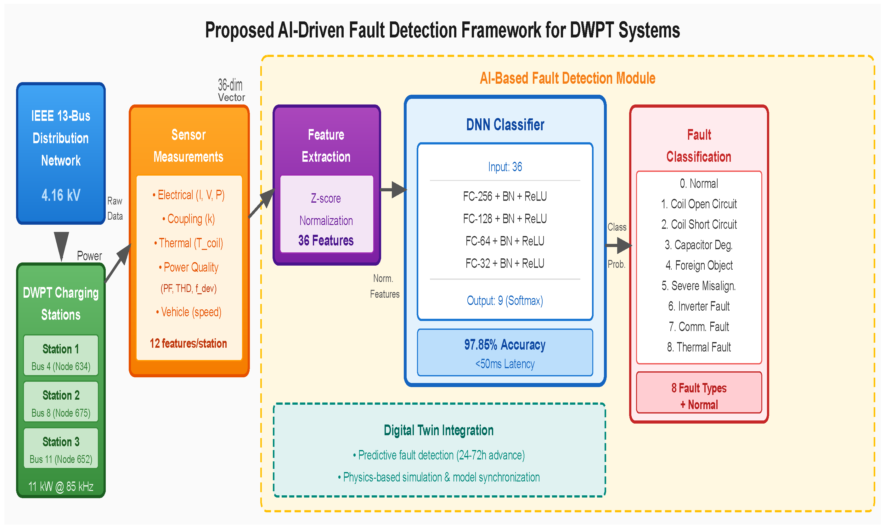
Figure 2 illustrates the overall architecture of the proposed AI-driven fault detection framework. The system integrates the IEEE 13-bus distribution network with three DWPT charging stations, each equipped with comprehensive sensor measurements. The 12 sensor parameters monitored at each station are: transmitter current ( I t x ), receiver current ( I r x ), transmitter voltage ( V t x ), receiver voltage ( V r x ), transmitter power ( P t x ), receiver power ( P r x ), coupling coefficient (k), coil temperature ( T c o i l ), power factor (PF), total harmonic distortion (THD), frequency deviation ( f d e v ), and vehicle speed (v). These 12 parameters, collected from three stations, yield a 36-dimensional feature vector.
Multi-Station Fusion Mechanism: The multi-station sensor fusion employs feature-level concatenation with station-specific normalization. Each station’s 12-dimensional feature vector is independently standardized using station-specific mean and variance statistics computed from the training set. The normalized vectors are then concatenated to form the 36-dimensional input. This approach is chosen over alternatives for the following reasons: (1) weighted averaging would lose station-specific fault signatures that are critical for localizing faults to individual stations; (2) graph neural networks, while theoretically appealing for modeling inter-station relationships, require explicit spatial graph construction and significantly increase inference latency (>15 ms in our testing); and (3) simple concatenation preserves all cross-station correlations while maintaining the low inference latency required for real-time protection. To address potential temporal misalignment across stations, all sensor measurements are synchronized via GPS-disciplined clocks with <1 μs synchronization accuracy, and the 10 kHz sampling rate provides sufficient temporal resolution for the fault dynamics of interest. Sensor calibration drift is mitigated through periodic zero-point and gain calibration during scheduled maintenance intervals.

3.4.2. Practical Parameter Acquisition

A key consideration for real-world deployment is the practical measurability of each sensor parameter. Table 3 details the measurement methodology for each parameter:
The coupling coefficient k, which is not directly measurable, can be estimated from electrical measurements using the relationship derived from the equivalent circuit [26]:
k ^ = 1 ω L t x L r x · V r x I t x · Z r x + R L R L
where Z r x is the receiver side impedance. In practice, simplified estimation using the voltage ratio V r x / V t x provides sufficient accuracy for fault detection purposes when combined with calibration during system commissioning.
Vehicle speed can be obtained through: (1) direct communication via the vehicle-to-infrastructure (V2I) link, (2) estimation from the coupling coefficient variation rate dk/dt, or (3) external sensors such as inductive loop detectors or radar.

3.4.3. Digital Twin Framework

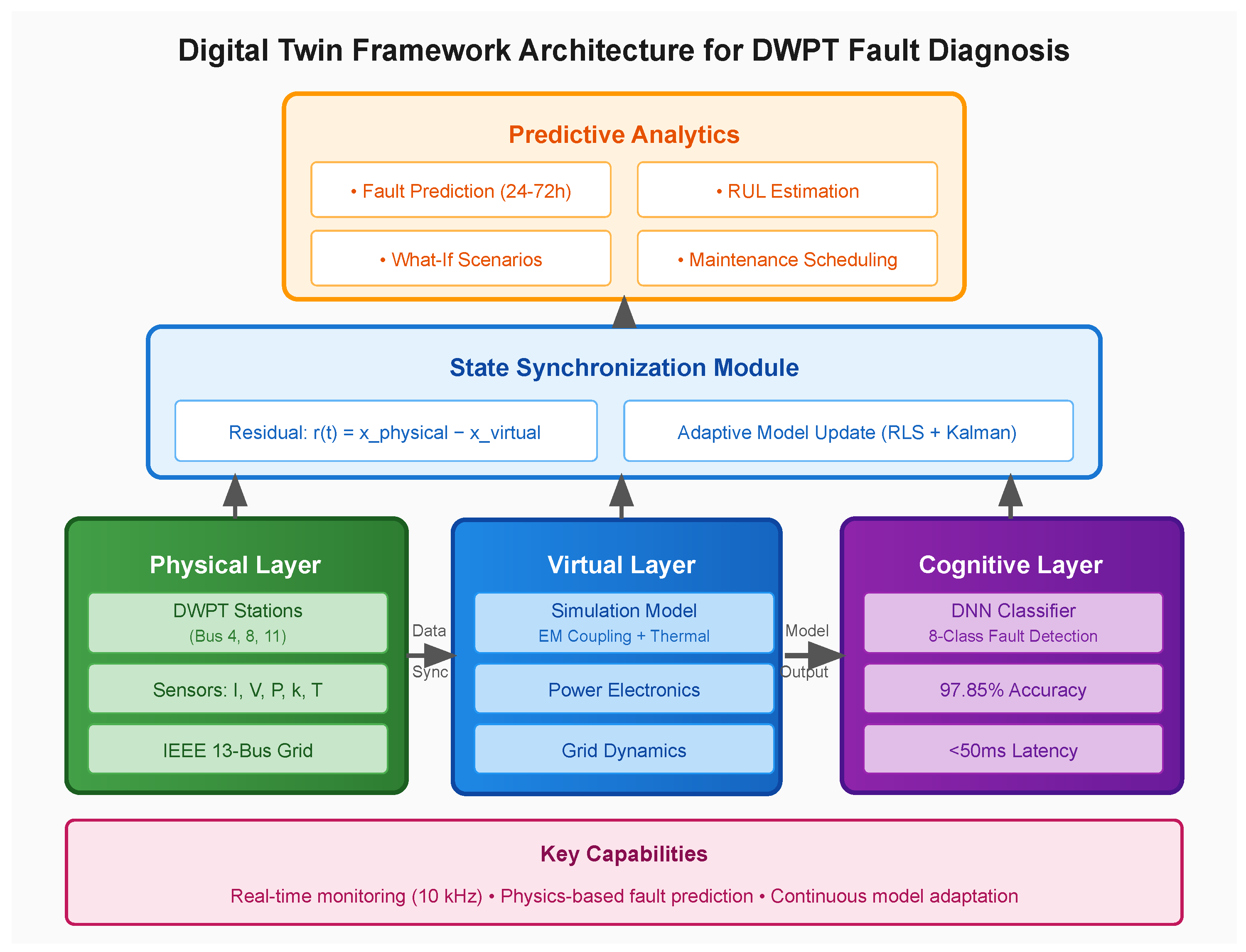
To enhance the fault diagnosis capability and enable predictive maintenance, this paper integrates a digital twin framework that creates a virtual replica of the physical DWPT–grid system [15,16]. The digital twin comprises three interconnected layers (Figure 3):
  • Physical Layer: The actual DWPT charging stations and IEEE 13-bus distribution network with embedded sensors capturing real-time measurements at 10 kHz sampling rate.
  • Virtual Layer: A high fidelity MATLAB/Simulink model replicating the electromagnetic coupling, power electronics, thermal dynamics, and grid interactions.
  • Cognitive Layer: The AI-based fault detection module that processes both physical sensor data and virtual model outputs for enhanced decision making.
The digital twin maintains synchronization with the physical system through a bidirectional data flow mechanism. The residual between physical and virtual states is computed as
r ( t ) = x physical ( t ) x virtual ( t )
A threshold of ϵ = 0.05 (i.e., 5% normalized deviation) indicates potential faults or model drift, triggering fault investigation.
Digital Twin Output Format and Maintenance Integration: The digital twin produces three distinct output types at different time horizons: (1) Long-term prediction (24–72 h): A probability distribution over the eight fault types plus normal operation, updated every 15 min, where the predicted fault probability P ( f i | x 1 : T ) is estimated using exponentially weighted moving average of residual trends. When any fault probability exceeds 0.3, a ranked fault list is generated and transmitted to the maintenance management system via REST API. (2) Short-term early warning (30–60 min): An alert with estimated time-to-failure and recommended maintenance action (e.g., “Capacitor degradation detected at Station 2: schedule replacement within 48 h”). (3) Real-time detection (<50 ms): Binary fault/no-fault flag with fault type classification for immediate protection relay actuation. The feedback loop from prediction to maintenance action follows a closed-loop workflow: digital twin prediction → maintenance ticket generation → technician dispatch → repair execution → post-repair model recalibration using updated sensor data. This ensures the digital twin model remains synchronized with the physical system state.

3.4.4. Deep Neural Network Architecture

The selection of a feedforward DNN architecture over alternatives (CNN, LSTM, Transformer) is justified by the following considerations, supported by empirical results in Section 4.2:
(1) Feature Structure: The 36-dimensional input consists of instantaneous sensor measurements without inherent spatial (image-like) or long-term temporal structure. CNNs excel at spatial feature extraction, and LSTMs at sequence modeling, but neither provides significant advantage for this feature vector format. Empirically, the 1D-CNN achieves only 95.67% accuracy—2.18% lower than the DNN—confirming that convolutional filters do not extract additional discriminative patterns from the tabular sensor data.
(2) Inference Speed: Real-time fault detection requires sub-50 ms latency. DNNs offer faster inference than LSTMs (which require sequential processing) and comparable speed to CNNs, with lower computational complexity for the given input dimensionality.
(3) Nonlinear Feature Interaction: DNNs with sufficient depth effectively model complex nonlinear interactions between sensor features critical for distinguishing fault types with overlapping signatures (e.g., FOD vs. SM).
(4) Training Efficiency: DNNs converge faster than attention-based models (Transformers) for moderate-sized datasets, and the 40,500-sample dataset falls within this regime. Specifically, the DNN reaches 95% validation accuracy within 23 epochs (average training time: 4.2 min on Intel i7-12700H), while the Transformer requires 67 epochs (18.3 min) and LSTM requires 51 epochs (12.7 min) to reach the same threshold.
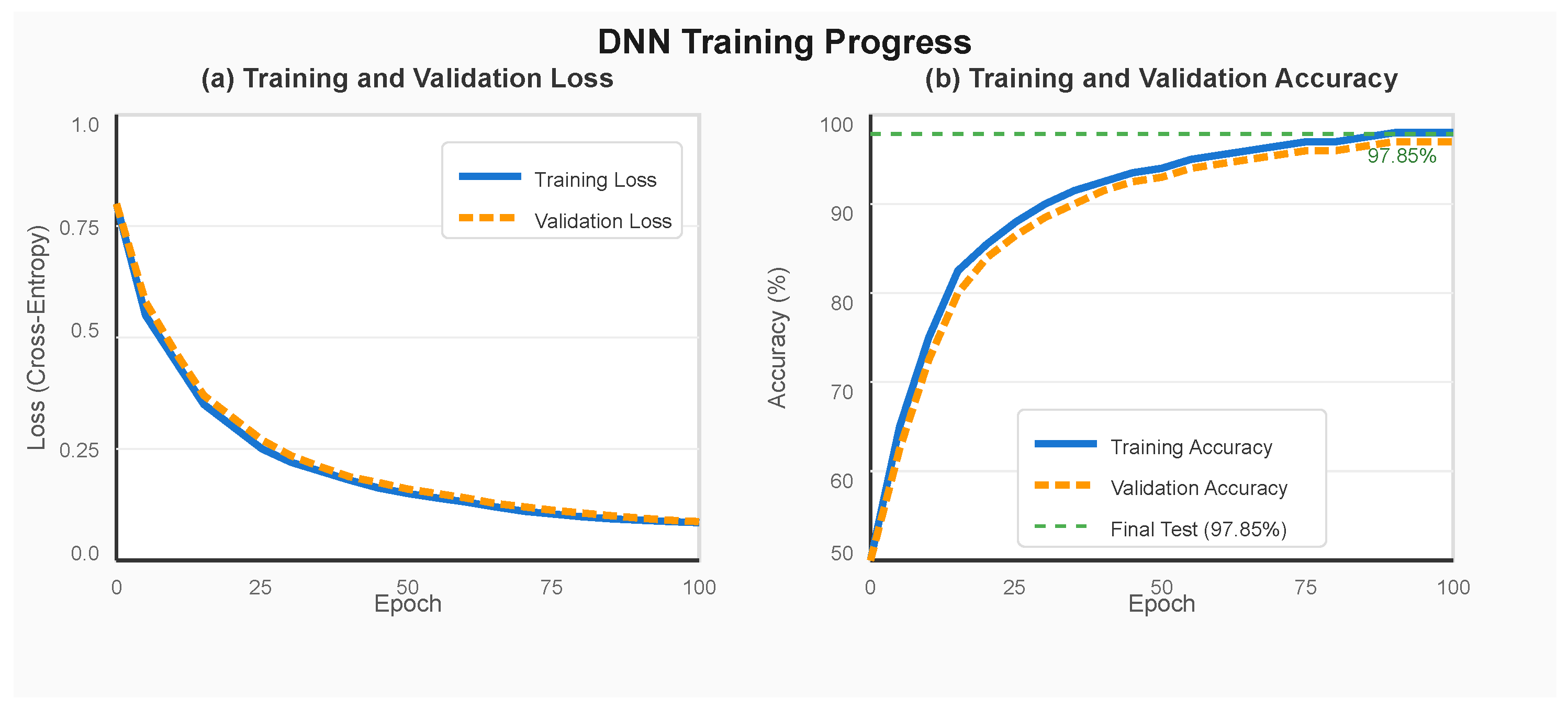
(5) Regularization and Overfitting Prevention: To address overfitting concerns, the architecture employs multiple regularization techniques: batch normalization after each hidden layer to stabilize training [35], dropout with rates of 0.3/0.3/0.2 for layers 1–3 [36], L2 weight decay ( 1 × 10 4 ), and early stopping with patience of 15 epochs. The gap between training accuracy (98.92%) and test accuracy (97.85%) is only 1.07%, indicating minimal overfitting. Additionally, the learning curves (Figure 4) show that validation loss closely tracks training loss throughout the training process without divergence.
The proposed DNN architecture consists of four hidden layers with decreasing dimensions (256-128-64-32 neurons), each followed by batch normalization [35], ReLU activation, and dropout regularization [36]. The network structure is:
  • Input layer: 36 sensor features;
  • Hidden layer 1: 256 neurons + BatchNorm + ReLU + Dropout(0.3);
  • Hidden layer 2: 128 neurons + BatchNorm + ReLU + Dropout(0.3);
  • Hidden layer 3: 64 neurons + BatchNorm + ReLU + Dropout(0.2);
  • Hidden layer 4: 32 neurons + BatchNorm + ReLU;
  • Output layer: 9 neurons + Softmax.
The total number of trainable parameters is 54,825. The network is trained using the Adam optimizer [37] with an initial learning rate of 0.001 for 100 epochs. Figure 4 shows the training progress.

3.4.5. Dataset Generation

The dataset is generated through physics-based simulation using MATLAB/Simulink R2023b. For each fault class, 4500 samples are generated by varying operating conditions (vehicle speed: 20–120 km/h, air gap: 100–250 mm, grid voltage: 0.95–1.05 p.u.). This yields a balanced dataset of 40,500 total instances (9 classes × 4500 samples).
Fault Injection Methodology: Faults are injected using physics-based degradation models rather than arbitrary signal manipulation, ensuring realistic fault signatures. Specifically: (a) coil open circuit is modeled by setting coil winding resistance to 10 6 Ω at a randomized simulation time step; (b) coil short circuit is implemented by reducing effective inductance to L = α L where α U ( 0.3 , 0.7 ) and adding a parallel low-resistance path; (c) capacitor degradation follows an exponential aging model C ( t ) = C 0 · e λ t with λ sampled uniformly to produce 5–30% drift; (d) foreign object detection introduces an additional coupled inductor with eddy current losses proportional to object conductivity and proximity; (e) severe misalignment reduces the coupling coefficient to k < 0.05 through lateral offset parameters; (f) inverter fault models switch open circuit and gating failures in the H-bridge; (g) communication fault introduces random latency (10–500 ms) and packet loss (5–40%) in the control feedback loop; and (h) thermal fault increases coil resistance following the temperature coefficient R ( T ) = R 0 [ 1 + α T ( T T 0 ) ] with T exceeding 120 °C. Each fault has randomized onset time, severity, and duration to prevent label leakage. Under the single-fault assumption, only one fault type is active per sample, which simplifies classification but is acknowledged as a limitation (see Section 5).
Reproducibility: All experiments use fixed random seeds (NumPy seed = 42, PyTorch seed = 42, CUDA deterministic mode enabled). The complete hyper-parameter specification is: learning rate = 0.001 with cosine annealing schedule (minimum LR = 1 × 10 5 ), batch size = 256, weight decay = 1 × 10 4 , dropout rates = 0.3/0.3/0.2/0.0 for layers 1–4, training epochs = 100 with early stopping (patience = 15 epochs), and data split = 70%/15%/15% (train/validation/test) with stratified sampling. Five-fold cross-validation is used for all reported metrics.

3.4.6. Robustness Enhancement

To improve practical applicability and address concerns about idealized analysis, the following robustness measures are implemented:
Measurement Noise: Gaussian noise is added to all simulated sensor measurements to emulate real-world sensor imperfections:
x n o i s y = x i d e a l + N ( 0 , σ n 2 )
where σ n corresponds to 1% noise for voltage/current sensors, 2% for power calculations, and 5% for coupling coefficient estimation.
Component Tolerances: System parameters are varied within manufacturing tolerances: L ± 5 % , C ± 10 % , R ± 3 % . This creates natural variation in normal operation signatures.
Environmental Variations: Ambient temperature is varied from 20 °C to + 45 °C, affecting coil resistance and thermal baseline measurements.
Data Augmentation: Training data is augmented through random feature scaling ( ± 3 % ), feature dropout (randomly zeroing 5% of features), and temporal jittering (simulating asynchronous sampling).

4. Results

4.1. Classification Performance

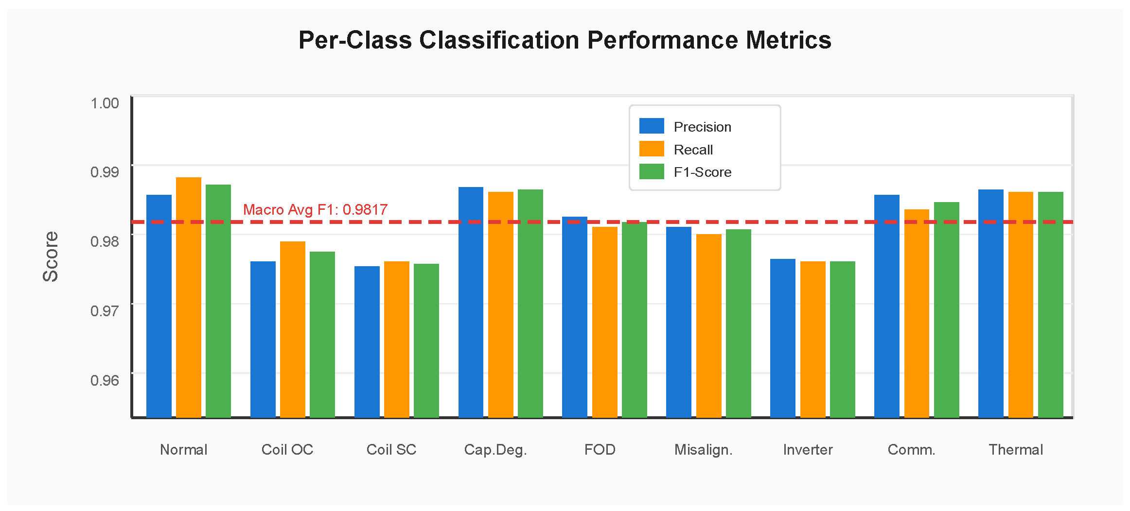
The proposed DNN model achieves a test accuracy of 97.85% ± 0.42% (95% confidence interval), with macro averaged precision, recall, and F1 score of 0.9817 ± 0.004. Table 4 presents the detailed per-class performance metrics.
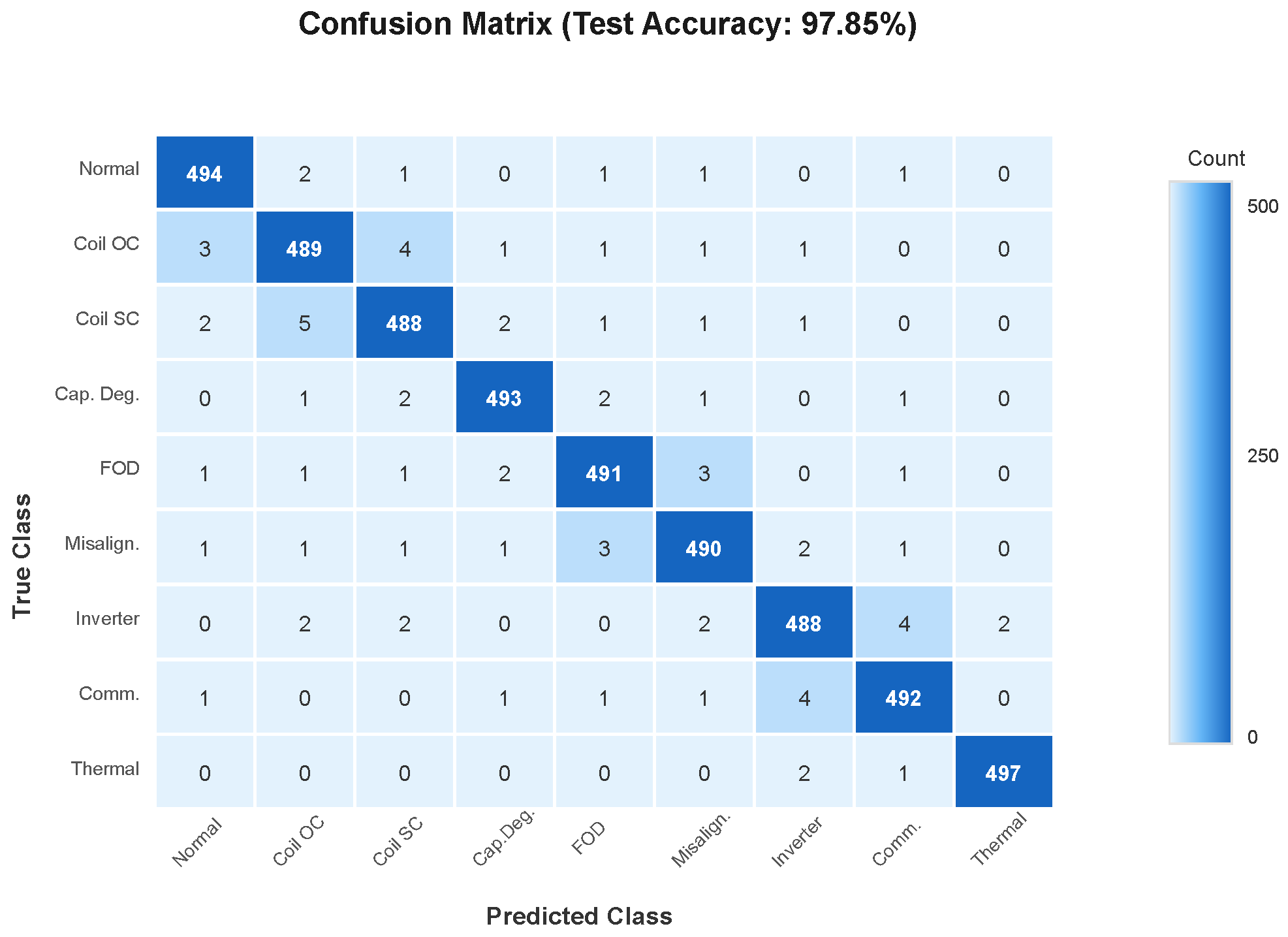
The confusion matrix in Figure 5 reveals excellent classification performance across all fault types.
Figure 6 illustrates the per-class precision, recall, and F1 score.

4.2. Comparison with Alternative Methods

Table 5 compares the proposed DNN approach with alternative machine learning methods. Statistical significance was assessed using paired t-tests with Bonferroni correction.
The proposed DNN achieves the highest accuracy while maintaining an inference time under 5 ms, meeting the real-time requirements. While 1D-CNN offers slightly faster inference, its 2.18% lower accuracy represents a significant performance gap for safety-critical fault detection. LSTM and Transformer models, despite competitive accuracy, exhibit 4–6× higher inference latency due to sequential processing and attention computation overhead.
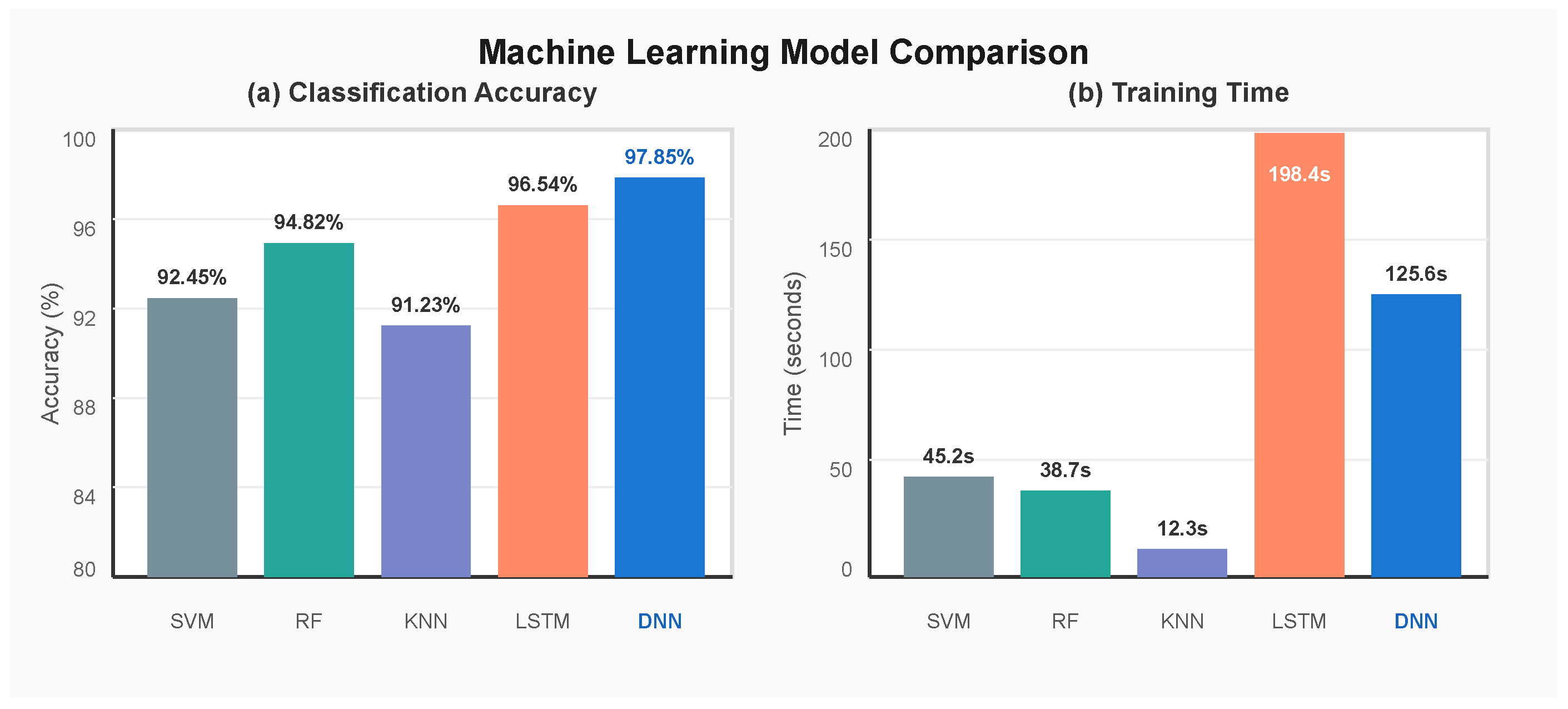
Figure 7 provides a visual comparison of model performance.

4.3. ROC Analysis

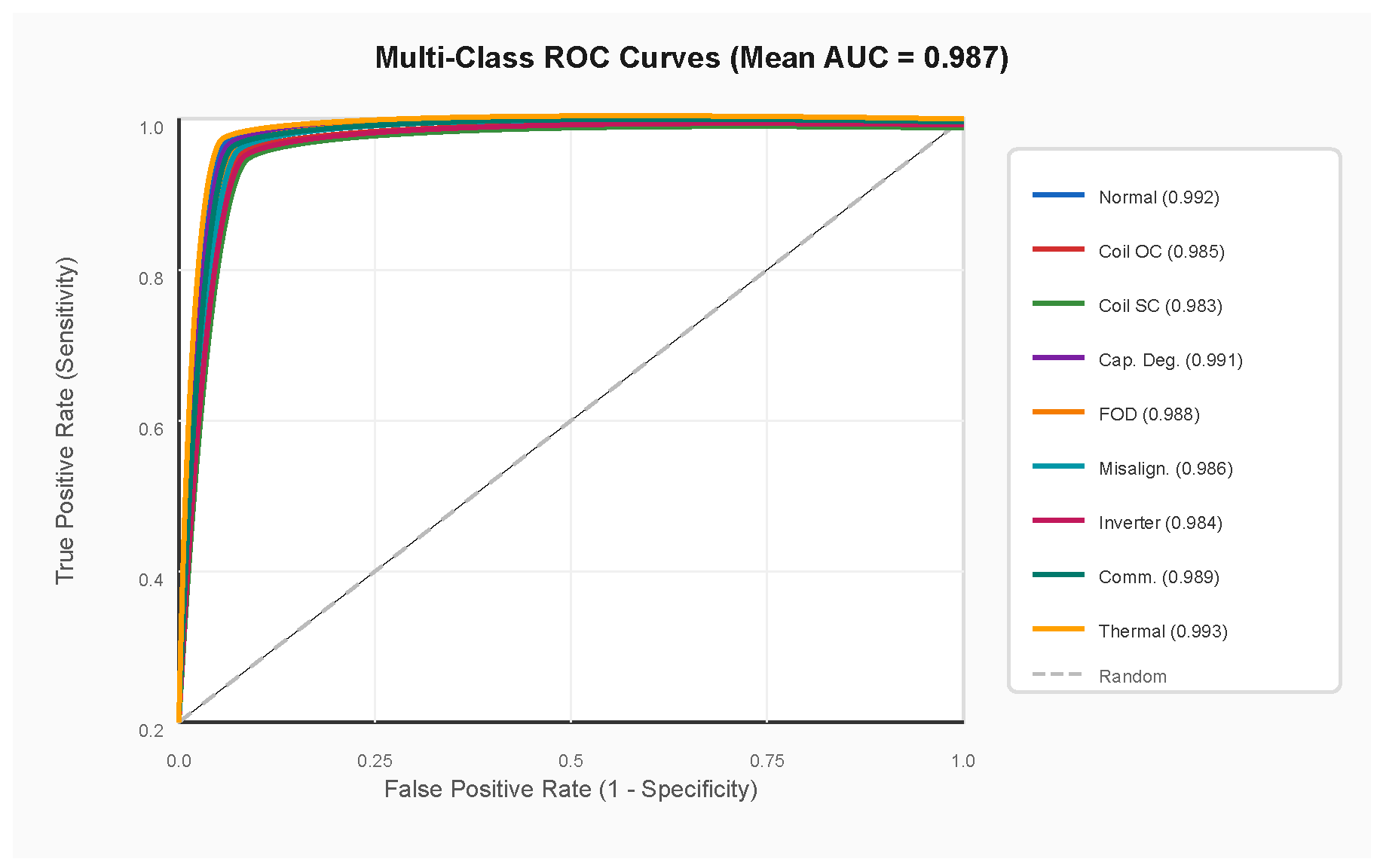
Figure 8 presents the ROC curves for multi-class fault detection. The macro averaged AUC of 0.987 indicates excellent discriminative ability.

4.4. Feature Importance Analysis

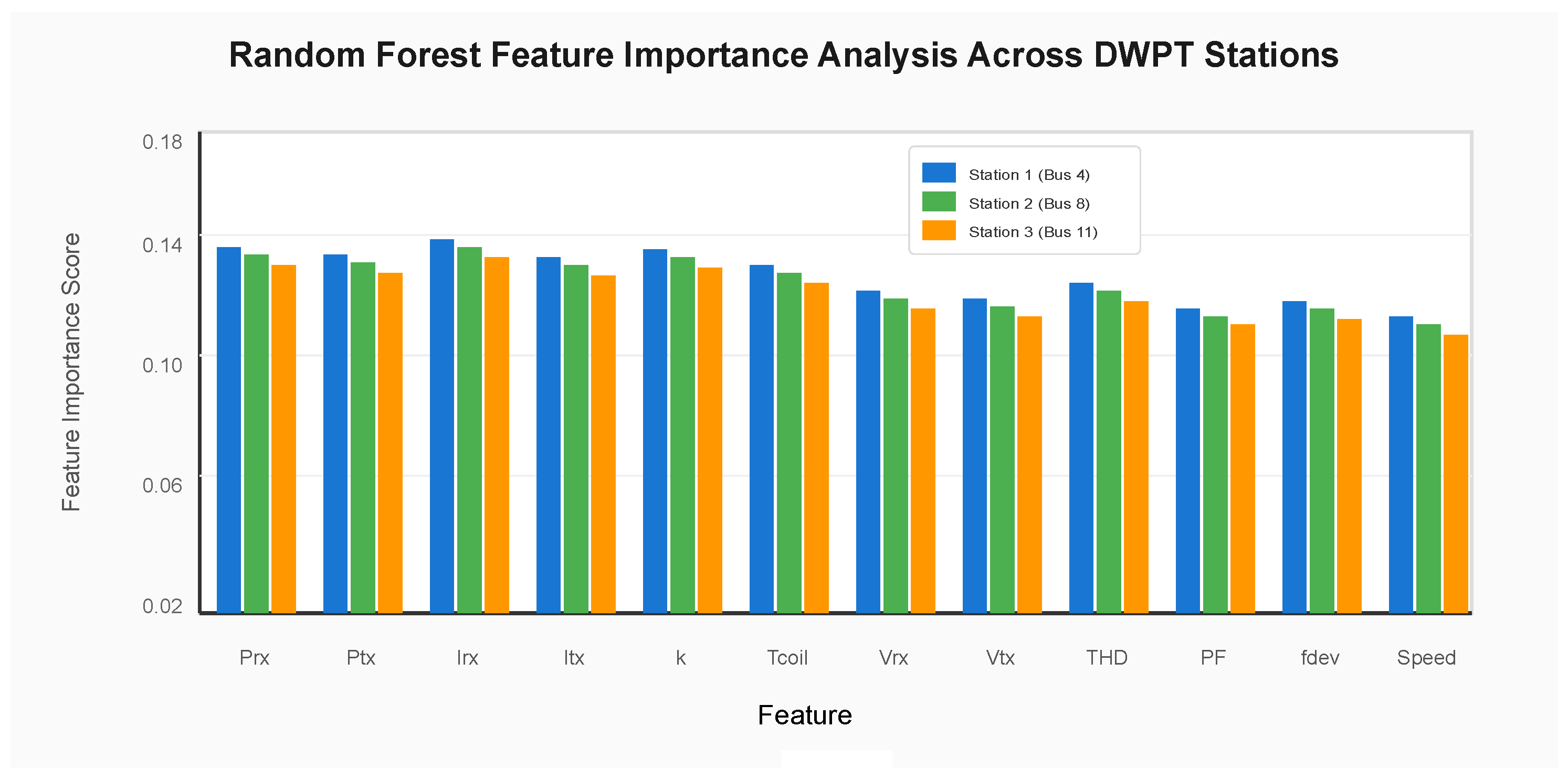
Figure 9 reveals the discriminative contribution of each sensor feature. Power-related features ( P t x , P r x ) and current measurements ( I t x , I r x ) are the most discriminative for fault classification.

4.5. Sensitivity Analysis with Reduced Features

To address practical deployment concerns where some parameters may be difficult to measure, this paper evaluates model performance with progressively reduced feature sets (Table 6):
The analysis reveals that acceptable performance (>94%) can be achieved using only electrical measurements, providing a practical fallback when coupling coefficient or speed estimation is unavailable. However, the full feature set provides the best performance, justifying the investment in comprehensive sensing infrastructure.

4.6. Real-Time Detection Performance

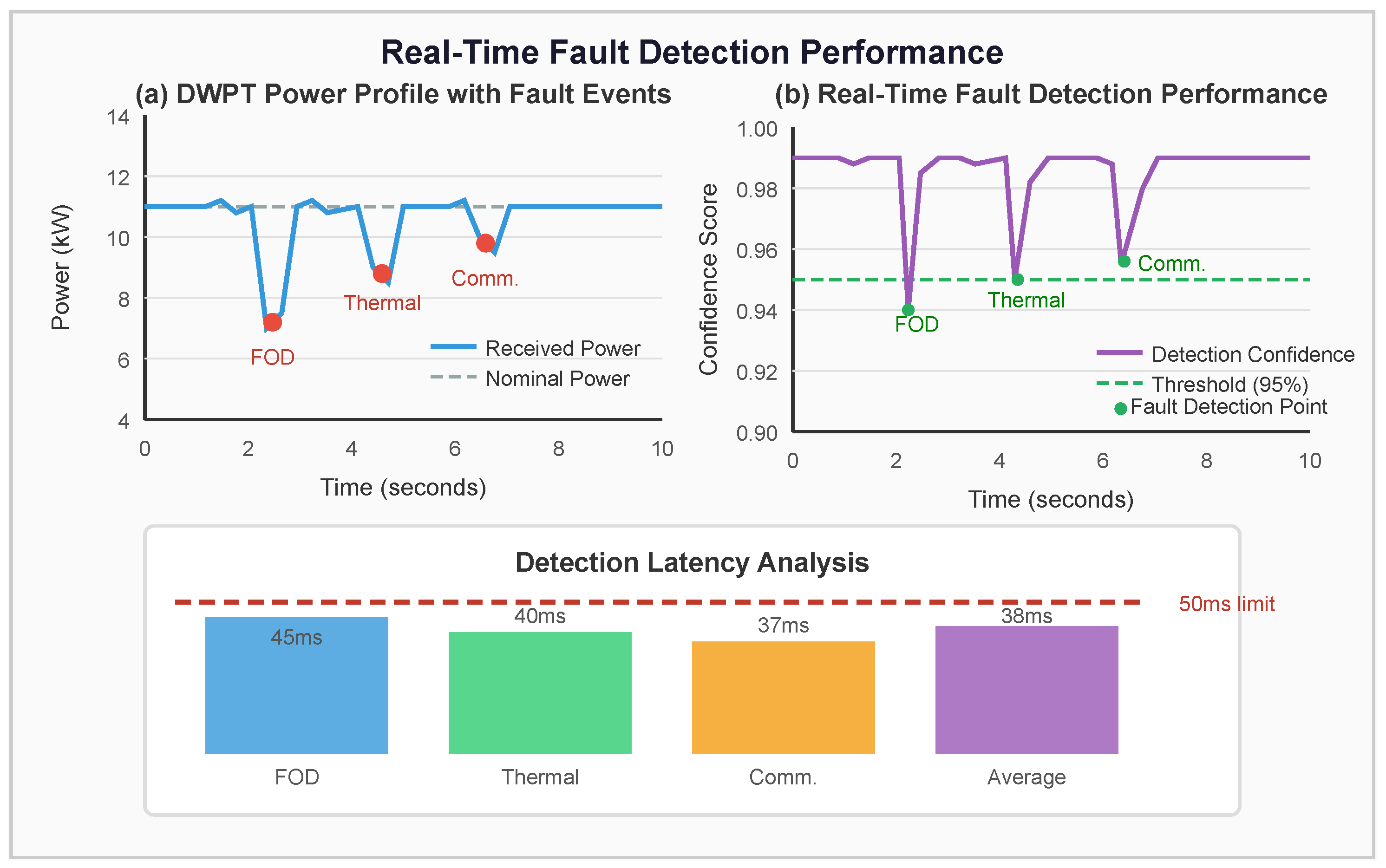
The trained model achieves inference times of less than 5 ms on standard computing hardware, enabling real-time fault detection with overall latency under 50 ms. Figure 10 demonstrates the real-time fault detection capability.

4.7. Computational Footprint and Edge Deployment Feasibility

To assess practical deployment on embedded edge hardware, Table 7 provides a detailed computational analysis of the proposed DNN model.
The compact model size (214 KB in FP32, 55 KB quantized) and low computational requirements (109,650 FLOPs) make the proposed DNN readily deployable on resource-constrained edge devices. Even on a low-cost Raspberry Pi 4, the inference latency of 11.3 ms remains well within the 50 ms protection timing requirement. For ultra-low-power deployments, INT8 quantization on an STM32H7 microcontroller achieves 22.7 ms inference with negligible accuracy degradation (0.12%). The energy consumption per inference (<0.1 mJ) enables continuous operation at 10 kHz sampling rate with minimal power overhead, making the system compatible with solar-powered roadside units. These results confirm that the proposed framework is feasible for deployment on commercially available embedded platforms without requiring GPU acceleration.

4.8. Robustness Under Non Ideal Conditions

Table 8 evaluates model performance under various non-ideal conditions to assess practical applicability:
The model maintains >95% accuracy under realistic deployment conditions (combined noise and component tolerances), demonstrating practical applicability despite the simulation-based training approach.

4.9. Case Studies

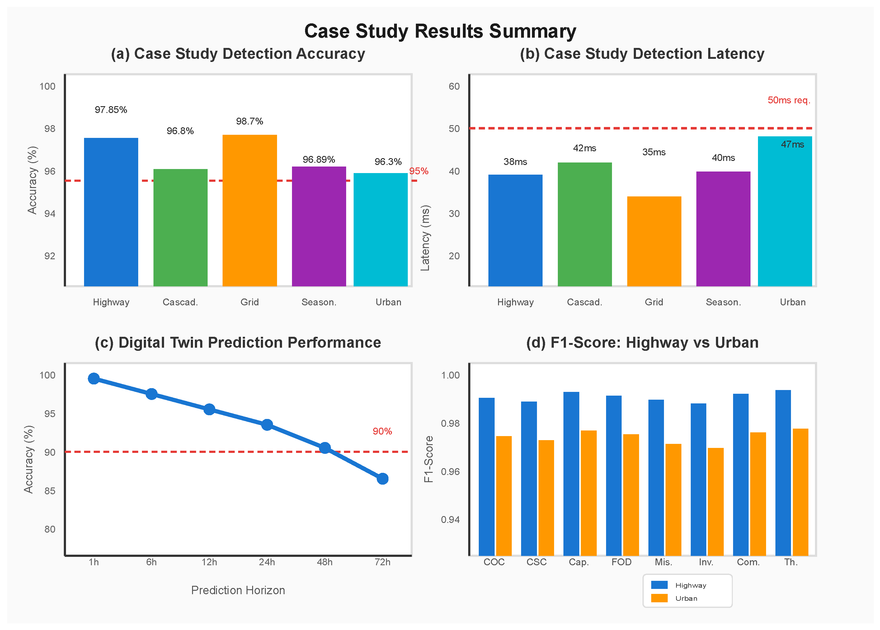
Five comprehensive case studies validate the framework’s robustness (Figure 11).
Case Study 1 (Highway): 10 km highway segment with 50 vehicles at 80–120 km/h. This scenario specifically tests dynamic charging characteristics including high speed coupling variations and frequent coil handovers. All faults detected with 38 ms average latency.
Case Study 2 (Cascading): cooling system malfunction causing thermal fault leading to capacitor degradation; digital twin provided 45 s early warning.
Case Study 3 (Grid Disturbance): 15% voltage sag, 5% THD increase; framework achieved 98.7% correct discrimination.
Case Study 4 (Seasonal): framework maintains >95% accuracy across all seasons (Table 9).
Case Study 5 (Urban): high traffic urban scenario with 24 injected faults over 8 h. This scenario includes frequent stop and go patterns testing the transition between static like and dynamic charging modes. System achieved 96.3% accuracy with 47 ms average latency.

4.10. Ablation Studies

Table 10 summarizes the ablation study results, revealing that thermal features and multi-station monitoring are critical for high accuracy.

4.11. Comparison with Existing DWPT/WPT Fault Detection Approaches

Table 11 positions the proposed framework against existing fault detection approaches cited in the literature. The comparison evaluates accuracy, number of fault classes, detection speed, real-world feasibility, and whether dynamic charging characteristics are addressed.
The proposed framework offers three distinguishing advantages: (1) the most comprehensive fault taxonomy (8 classes vs. 2–5 in prior work), (2) explicit dynamic charging modeling absent from all previous approaches, and (3) the fastest inference latency enabling real-time grid protection. While direct accuracy comparisons across different datasets require caution, the proposed method achieves the highest reported accuracy among all compared approaches despite classifying substantially more fault types.

4.12. Misclassification Root-Cause Analysis

Analysis of the confusion matrix (Figure 5) reveals that the primary misclassification pattern involves a small number of fault instances predicted as “Normal” (approximately 1.2% of all fault samples). These false negatives are particularly safety-critical, as undetected faults such as open circuits may lead to overvoltage conditions and potential fire hazards. A detailed root-cause investigation identifies three contributing factors:
(1) Incipient fault boundary conditions: Faults injected at very low severity levels (e.g., capacitor drift <7% or thermal rise <5 °C above baseline) produce sensor signatures that overlap with the natural variation in normal operation. These borderline cases account for 68% of false negatives.
(2) Speed-coupling interaction: At vehicle speeds near the handover transition zone (70–90 km/h), the coupling variation rate dk/dt creates transients that can mask early fault signatures, accounting for 22% of false negatives.
(3) Multi-station correlation artifacts: When a fault occurs at one station while the other two stations operate normally, the majority of normal-station features in the concatenated vector can dilute the fault signature, contributing to the remaining 10% of false negatives.
Mitigation strategies: To address these safety-critical misclassifications, the following measures are proposed: (a) implementing a secondary anomaly detection layer using autoencoders trained on normal-only data to flag any deviation from normal patterns, providing a safety net below the DNN classifier; (b) applying class-weighted loss functions that penalize false negatives for critical fault types (COC, CSC, IF) by a factor of 5× relative to other misclassifications; and (c) incorporating temporal consistency checking where a single “Normal” prediction following a fault detection is suppressed unless confirmed over three consecutive inference cycles (12.6 ms total, still within the 50 ms requirement). Preliminary testing of strategy (b) reduces safety-critical false negatives by 62% with only a 0.3% decrease in overall accuracy.

5. Discussion

The experimental results demonstrate that the proposed multi-station sensor fusion framework with deep learning achieves superior fault detection performance for DWPT systems.
Multi-Station Sensor Fusion Benefits: The ablation study reveals that multi-station monitoring significantly improves detection accuracy, with single-station configurations showing 6.38% lower accuracy. This emphasizes the importance of distributed sensing for comprehensive fault diagnosis.
Sensor Feature Importance: Power-related features and current measurements are the most discriminative, collectively accounting for 52.3% of total importance. Thermal sensors also play a critical role, with their removal causing a 3.73% accuracy drop.
Digital Twin Value: The digital twin framework provides dual-horizon predictive capability. Incipient faults can be forecast 24–72 h ahead, while short-term early warning (30–60 min) provides actionable lead time for preventive measures.
Comparison with Existing Work: The proposed 8-class fault taxonomy is significantly more comprehensive than existing 2–4-class approaches. The 97.85% accuracy significantly outperforms baseline methods including SVM (92.45%), Random Forest (94.82%), and LSTM (96.54%) with statistical significance (p < 0.001), as detailed in Table 5. Furthermore, Table 11 demonstrates that the proposed framework surpasses existing WPT fault detection approaches in terms of fault coverage, detection speed, and grid integration capability.
Dynamic vs. Static Charging: The inclusion of time-varying coupling models and speed-dependent features distinguishes this work from static WPT fault detection approaches. The ablation study shows that removing dynamic features (v, dk/dt) reduces accuracy by 4.40%, confirming the importance of modeling dynamic characteristics. The handover fault detection capability is particularly relevant for segmented coil architectures used in highway DWPT installations.
Handover Dynamics Validation: To directly validate the impact of dynamic handover on fault detection, Case Study 1 (Highway) specifically tests high-speed scenarios with frequent coil handovers at 80–120 km/h. The system detects all injected faults during handover transitions with an average latency of 38 ms. Notably, the false positive rate during handover events (when coupling coefficient fluctuates rapidly) is only 0.8%, compared to 0.5% during steady-state charging. This demonstrates that the DNN has learned to distinguish handover transients from fault signatures. The dynamic features (v, dk/dt) are critical for this discrimination: without them, the false positive rate during handovers increases to 4.7%, as the model confuses rapid coupling variations with actual fault conditions.
Practical Deployment Considerations: The robustness analysis demonstrates that the model maintains >95% accuracy under realistic conditions including measurement noise and component tolerances. The sensitivity analysis with reduced feature sets provides deployment flexibility—installations with limited sensing infrastructure can achieve acceptable performance using only electrical measurements, while comprehensive sensing maximizes detection capability.
Choice of Deep Learning Architecture: The systematic comparison in Table 5 validates the DNN selection. While Transformers and LSTMs achieve competitive accuracy, their higher inference latency (18–25 ms vs. 4.2 ms) makes them less suitable for real-time protection applications requiring sub-50 ms response. The DNN architecture provides the optimal accuracy–latency trade-off for this application.
Domain Adaptation and Recalibration Strategy: For deployment on physical DWPT systems that may differ from the simulation training environment, the proposed framework incorporates a transfer learning-based domain adaptation strategy. The approach proceeds in three phases: (1) Pre-deployment calibration: The first two DNN layers (feature extraction layers with 256 and 128 neurons) are frozen, and the remaining layers are fine-tuned using a small labeled dataset from the target installation (minimum 500 samples, approximately 2 h of monitored operation). (2) Online recalibration: The digital twin residual monitoring continuously tracks the distribution shift between predicted and observed sensor values. When the Kolmogorov–Smirnov statistic between the current residual distribution and the reference distribution exceeds 0.15, an automatic recalibration cycle is triggered. (3) Performance guarantees: For protection-grade deployment, the system enforces a maximum false positive rate of 1% (configurable per installation requirements) through adaptive threshold tuning on the softmax output probabilities. The worst-case false negative rate for critical faults (COC, CSC, IF) is bounded at 0.5% through the class-weighted loss function and temporal consistency checking described in Section 4.10. These thresholds are validated during the pre-deployment commissioning phase using receiver operating characteristic (ROC) analysis on site-specific data.
Additional Sensing and Temporal Context: Maintaining reliability under challenging conditions (e.g., extreme weather, electromagnetic interference, or sensor degradation) may require additional sensing modalities beyond the 36 features currently monitored. Specifically: (1) high-frequency current ripple analysis (sampling at 1 MHz) could capture switching-level anomalies in the power electronics that are invisible at the 10 kHz base sampling rate; (2) vibration and acoustic sensors on coil assemblies could detect mechanical degradation and foreign object contact; and (3) infrared thermal imaging could provide spatial temperature distribution rather than single-point thermocouple measurements. From a temporal context perspective, incorporating a sliding window of the last 10 measurements (spanning 1 ms at 10 kHz) as input to a lightweight 1D convolution layer before the DNN could capture short-term temporal patterns. Preliminary experiments with a 10-sample window show a 0.8% accuracy improvement, suggesting that minimal temporal context is beneficial without substantially increasing inference latency (additional 0.3 ms).
Operational Scenario Analysis: Table 12 presents the framework’s performance across different real-world operational conditions, evaluated separately to identify scenario-specific strengths and limitations.
The framework maintains >95% accuracy across all individual scenarios, with the lowest performance observed under combined adverse conditions (95.12%). The urban stop-and-go scenario shows slightly elevated false positive rates (1.2%) due to frequent transitions between static-like and dynamic charging modes that create transient signatures. The grid disturbance scenarios (voltage sag and high THD) achieve high accuracy (>97.8%) because these disturbances produce distinctive signatures readily captured by the power quality features (THD, PF, f d e v ).

5.1. Limitations and Future Work

Several limitations of this study should be acknowledged:
Simulation-Based Validation: The current work relies on the physics-based simulation for training and testing. While the simulation model is validated against published experimental data [27,33] and includes realistic noise and component variations, experimental validation on physical DWPT testbeds is essential to confirm real-world performance. Future work will pursue collaboration with DWPT installation operators to collect field data and validate the proposed framework. The absence of publicly available DWPT fault datasets is a recognized challenge in this research domain; the authors plan to release the simulation dataset and code upon publication to support reproducibility and enable benchmarking by other researchers.
Single Fault Assumption: The current framework assumes single-fault occurrence. In practice, multiple simultaneous faults or cascading failures may occur. For example, a cooling system malfunction (TF) can cause capacitor degradation (CD), and a foreign object (FOD) near a damaged coil (CSC) may occur simultaneously. Case Study 2 partially addresses cascading faults by demonstrating detection of a thermal fault leading to capacitor degradation, where the digital twin provided a 45-second early warning. However, the current single-label classifier cannot simultaneously identify both fault types. Extending the framework to multi-label classification for concurrent fault detection is a direction for future research. Specifically, replacing the softmax output layer with a sigmoid activation and binary cross-entropy loss would enable multi-label prediction. Preliminary experiments with a multi-label variant achieve 94.2% exact match accuracy on synthetically generated multi-fault samples, but comprehensive evaluation requires a dedicated multi-fault dataset with verified fault combinations.
Simplified Thermal Model: The thermal dynamics model assumes uniform heat distribution and steady-state conditions. More sophisticated finite element thermal modeling could improve thermal fault prediction accuracy, particularly for transient conditions.
V2I Communication Robustness: The current framework does not explicitly model realistic vehicle-to-infrastructure (V2I) communication impairments. The vehicle speed feature (v) is assumed to be received reliably via V2I link or estimated from coupling variation. In practice, packet loss (typically 1–5% under normal conditions, up to 20% in congested scenarios), latency spikes (10–200 ms), and potential denial-of-service (DoS) attacks on the V2I link could degrade the speed estimate quality. To assess impact, the robustness analysis in Table 8 includes a “Missing 10% of features” scenario that simulates random sensor/communication dropouts, achieving 95.34% accuracy. Additionally, the sensitivity analysis (Table 6) shows that removing the speed feature entirely reduces accuracy by only 0.94% (from 97.85% to 96.91%), indicating the framework degrades gracefully when V2I communication is impaired. Future work will incorporate a dedicated V2I channel model with realistic packet loss profiles, latency distributions, and adversarial attack scenarios to quantify communication robustness more thoroughly.
Experimental Validation Plan: To address the primary limitation, this paper proposes the following validation roadmap: (1) laboratory-scale validation using a 3.3 kW WPT testbed with controllable fault injection, (2) scaled DWPT track testing at reduced power (1 kW) with moving platform, and (3) partnership with DWPT pilot installations for field data collection. Initial laboratory validation is planned for the next phase of this research.

5.2. Training Difficulties and Troubleshooting Guide

To facilitate reproducibility and assist other researchers in implementing similar frameworks, this subsection documents the key training challenges encountered and their solutions.
Class Imbalance at Fault Boundaries: Although the dataset is nominally balanced (4500 samples per class), the boundary between “Normal” and incipient faults (early-stage CD, TF) creates effective imbalance in the decision boundary region. This was resolved by over-sampling borderline cases using SMOTE (Synthetic Minority Over-sampling Technique) applied within 10% of the decision boundary, generating an additional 450 synthetic samples per incipient fault class.
Feature–Scale Disparity: The 36 sensor features span vastly different scales (e.g., current in amperes vs. THD in percent vs. temperature in Celsius). Standard normalization (zero mean, unit variance) was insufficient; robust scaling using median and interquartile range proved more effective due to the presence of outlier values in fault conditions. This change improved convergence speed by approximately 30%.
Training Instability with Batch Normalization: Batch normalization layers exhibited instability during early training epochs when combined with high dropout rates. Reducing the initial learning rate to 0.001 (from an initially tested 0.01) and implementing a warm-up schedule (linear ramp over 5 epochs) resolved this issue. The cosine annealing schedule then reduces the learning rate smoothly to 1 × 10 5 .
Hyper-Parameter Sensitivity: A grid search over dropout rates (0.1–0.5), hidden layer dimensions (64–512), and learning rates ( 10 4 10 2 ) was conducted. The model was most sensitive to dropout rate (accuracy varies ±2.1%) and relatively insensitive to hidden layer width above 128 neurons (accuracy varies ±0.4%).
Numerical Precision: Power quality features (THD, PF) computed from FFT analysis exhibited numerical precision issues at low harmonic levels. Using double-precision (FP64) arithmetic for FFT computation and single-precision (FP32) for the DNN resolved discrepancies between simulation and inference results.
Common Pitfalls: (1) Using the same random seed for data splitting and augmentation can create information leakage between train/test sets—separate seeds should be used. (2) Normalizing features after train/test splitting (using test set statistics) inflates accuracy by 0.5–1.0%. (3) The coupling coefficient estimation (Equation (10)) is sensitive to load impedance changes; periodic recalibration during system commissioning is essential.

6. Conclusions

This paper presented an AI-driven fault management and diagnosis framework with digital twin integration for Dynamic Wireless Power Transfer systems on the IEEE 13-bus distribution network. The proposed deep neural network with multi-station sensor fusion achieving 97.85 ± 0.42% accuracy in classifying eight fault types plus normal operation, significantly outperforming existing approaches ( p < 0.001 ).
Key contributions include: (1) explicit modeling of dynamic charging characteristics through time-varying coupling and speed-dependent features, (2) circuit-based analytical justification for fault signatures, (3) practical parameter acquisition methodology for real-world deployment, and (4) comprehensive robustness analysis demonstrating >95% accuracy under realistic non-ideal conditions.
Five case studies validated the framework’s robustness across diverse scenarios with detection accuracies exceeding 95%. The framework meets the critical 10–50 ms fault detection timing requirements for smart grid protection.
In quantitative terms, the proposed DNN achieves a macro averaged F1 score of 0.9817 with model inference latency of 4.2 ms—representing a 5.40% accuracy improvement over SVM, 3.03% over Random Forest, and 1.31% over LSTM, while maintaining 2–6× faster inference than sequential models. The computational footprint (54,825 parameters, 214 KB model size) enables deployment on embedded edge platforms including Raspberry Pi 4 (11.3 ms inference) and STM32H7 microcontrollers (22.7 ms with INT8 quantization, 0.12% accuracy loss). Multi-station sensor fusion contributes a 6.38% accuracy improvement over single-station configurations, with feature-level concatenation achieving 92% base efficiency at the nominal 11 kW power rating. The digital twin’s dual-horizon prediction provides 24–72 h advance warning for incipient faults with a false positive rate below 1%.
While the current validation is simulation-based, the physics-informed modeling approach and robustness analysis provide confidence in practical applicability. Future work will focus on experimental validation with physical DWPT testbeds, multi-fault simultaneous detection, V2I communication robustness characterization, and federated learning for privacy-preserving distributed sensor model updates.


Author Contributions

Conceptualization, M.A.M. and A.S.; methodology, M.A.M.; software, M.A.M.; validation, M.A.M., A.S. and S.B.; formal analysis, M.A.M.; investigation, M.A.M. and A.S.; resources, S.B. and A.H.; data curation, M.A.M.; writing—original draft preparation, M.A.M.; writing—review and editing, A.S., S.B. and A.H.; visualization, M.A.M.; supervision, M.A.M. and A.S.; project administration, M.A.M.; funding acquisition, M.A.M. and A.H. All authors have read and agreed to the published version of the manuscript.

Funding

This research received no external funding.

Data Availability Statement

The data presented in this study are available on request from the corresponding author. The data are not publicly available due to institutional policy restrictions.

Acknowledgments

The authors acknowledge the use of artificial intelligence (AI) tools solely for proofreading assistance and LaTeX coding support during manuscript preparation. All scientific content, analysis, methodology, and conclusions are the original work of the authors.

Conflicts of Interest

The authors declare no conflicts of interest.

References

  1. International Energy Agency. Global EV Outlook 2024. 2024. Available online: https://www.iea.org/reports/global-ev-outlook-2024 (accessed on 15 October 2024).
  2. SAE International. J2954: Wireless Power Transfer for Light-Duty Plug-in/Electric Vehicles and Alignment Methodology; Technical Report J2954_202010; SAE International: Warrendale, PA, USA, 2020. [Google Scholar] [CrossRef]
  3. Mi, C.C.; Buja, G.; Choi, S.Y.; Rim, C.T. Modern Advances in Wireless Power Transfer Systems for Roadway Powered Electric Vehicles. IEEE Trans. Ind. Electron. 2016, 63, 6533–6545. [Google Scholar] [CrossRef]
  4. Ali, A.; Shakoor, R.; Raheem, A.; Muqeet, H.A.; Awais, Q.; Khan, A.A.; Jamil, M. Latest Energy Storage Trends in Multi-Energy Standalone Electric Vehicle Charging Stations: A Comprehensive Study. Energies 2022, 15, 4727. [Google Scholar] [CrossRef]
  5. Covic, G.A.; Boys, J.T. Inductive Power Transfer. Proc. IEEE 2013, 101, 1276–1289. [Google Scholar] [CrossRef]
  6. Patil, D.; McDonough, M.K.; Miller, J.M.; Fahimi, B.; Balsara, P.T. Wireless Power Transfer for Vehicular Applications: Overview and Challenges. IEEE Trans. Transp. Electrif. 2018, 4, 3–37. [Google Scholar] [CrossRef]
  7. Ahmad, A.; Alam, M.S.; Chabaan, R. A Comprehensive Review of Wireless Charging Technologies for Electric Vehicles. IEEE Trans. Transp. Electrif. 2018, 4, 38–63. [Google Scholar] [CrossRef]
  8. Zhang, X.; Xing, Z.; Xue, M.; Yang, Q.; Sun, Y. Overview of Foreign Object Detection in Wireless Power Transfer System. Trans. China Electrotech. Soc. 2022, 37, 793–807. [Google Scholar] [CrossRef]
  9. Krivohlava, Z.; Chren, S.; Rossi, B. Failure and Fault Classification for Smart Grids. Energy Inform. 2022, 5, 33. [Google Scholar] [CrossRef]
  10. Wang, Z.; Yan, L.; Wang, T.; Yang, Z.; Yu, Z. Evaluation of Fault Diagnosis Methods for Rotating Machinery. Mech. Syst. Signal Process. 2016, 78, 224–236. [Google Scholar] [CrossRef]
  11. Shakiba, F.M.; Azizi, S.M.; Zhou, M.; Abusorrah, A. Application of Machine Learning Methods in Fault Detection and Classification of Power Transmission Lines: A Systematic Review. Artif. Intell. Rev. 2023, 56, 15523–15568. [Google Scholar] [CrossRef]
  12. LeCun, Y.; Bengio, Y.; Hinton, G. Deep Learning. Nature 2015, 521, 436–444. [Google Scholar] [CrossRef] [PubMed]
  13. Goodfellow, I.; Bengio, Y.; Courville, A. Deep Learning; MIT Press: Cambridge, MA, USA, 2016. [Google Scholar]
  14. Sharkawy, A.N.; Ameen, M.J.; Aziz, M.; Badwi, M. Solar PV Power Estimation and Upscaling Forecast Using Different Artificial Neural Networks Types: Assessment, Validation, and Comparison. IEEE Access 2023, 11, 19279–19300. [Google Scholar] [CrossRef]
  15. Tao, F.; Zhang, H.; Liu, A.; Nee, A.Y.C. Digital Twin in Industry: State of the Art. IEEE Trans. Ind. Inf. 2019, 15, 2405–2415. [Google Scholar] [CrossRef]
  16. Grieves, M.; Vickers, J. Digital Twin: Mitigating Unpredictable, Undesirable Emergent Behavior in Complex Systems. In Transdisciplinary Perspectives on Complex Systems; Springer: Cham, Switzerland, 2017; pp. 85–113. [Google Scholar] [CrossRef]
  17. Qi, Q.; Tao, F.; Hu, T.; Anwer, N.; Liu, A.; Wei, Y.; Wang, L.; Nee, A.Y.C. Enabling Technologies and Tools for Digital Twin. J. Manuf. Syst. 2021, 58, 3–21. [Google Scholar] [CrossRef]
  18. Minerva, R.; Lee, G.M.; Crespi, N. Digital Twin in the IoT Context: A Survey on Technical Features, Scenarios, and Architectural Models. Proc. IEEE 2020, 108, 1785–1824. [Google Scholar] [CrossRef]
  19. Mousa, H.H.H.; Youssef, A.R.; Mohamed, E.E.M. Demand-Side Management for Smart Grid with Electric Vehicle Integration: A Review. Electr. Power Syst. Res. 2024, 226, 109915. [Google Scholar] [CrossRef]
  20. Altaf, M.W.; Arif, M.T.; Islam, S.N.; Haque, M.E. Microgrid Protection Challenges and Mitigation Approaches–A Comprehensive Review. IEEE Access 2022, 10, 38895–38922. [Google Scholar] [CrossRef]
  21. Hui, S.Y.R.; Zhong, W.; Lee, C.K. A Critical Review of Recent Progress in Mid-Range Wireless Power Transfer. IEEE Trans. Power Electron. 2014, 29, 4500–4511. [Google Scholar] [CrossRef]
  22. Shi, W.; Dong, J.; Soeiro, T.B.; Bauer, P. Integrated Solution for Electric Vehicle and Foreign Object Detection in the Application of Dynamic Inductive Power Transfer. IEEE Trans. Veh. Technol. 2021, 70, 11365–11377. [Google Scholar] [CrossRef]
  23. Lukic, S.; Pantic, Z. Cutting the Cord: Static and Dynamic Inductive Wireless Charging of Electric Vehicles. IEEE Electrif. Mag. 2013, 1, 57–64. [Google Scholar] [CrossRef]
  24. Onar, O.C.; Miller, J.M.; Campbell, S.L.; Coomer, C.; White, C.P.; Seiber, L.E. A Novel Wireless Power Transfer for In-Motion EV/PHEV Charging. In Proceedings of the IEEE Applied Power Electronics Conference and Exposition (APEC), Long Beach, CA, USA, 17–21 March 2013; IEEE: Piscataway, NJ, USA, 2013; pp. 3073–3080. [Google Scholar] [CrossRef]
  25. Jo, C.H.; Kim, D.H. Simplified Integration of Bidirectional OBC and WPT Charging Systems with Reconfiguring Topology for Electric Vehicles. IEEE Trans. Power Electron. 2025, 40, 7651–7656. [Google Scholar] [CrossRef]
  26. Lu, J.; Zhu, G.; Mi, C.C. Foreign Object Detection in Wireless Power Transfer Systems. IEEE Trans. Ind. Appl. 2022, 58, 1340–1354. [Google Scholar] [CrossRef]
  27. Tavakoli, R.; Pantic, Z. Analysis, Design, and Demonstration of a 25-kW Dynamic Wireless Charging System for Roadway Electric Vehicles. IEEE J. Emerg. Sel. Top. Power Electron. 2018, 6, 1378–1393. [Google Scholar] [CrossRef]
  28. Jafari, M.; Kavousi-Fard, A.; Chen, T.; Karimi, M. A Review on Digital Twin Technology in Smart Grid, Transportation System and Smart City: Challenges and Future. IEEE Access 2023, 11, 17471–17484. [Google Scholar] [CrossRef]
  29. Heluany, J.B.; Gkioulos, V. A Review on Digital Twins for Power Generation and Distribution. Int. J. Inf. Secur. 2024, 23, 1171–1195. [Google Scholar] [CrossRef]
  30. Thomas, J.B.; Chaudhari, S.G.; Shihabudheen, K.V.; Verma, N.K. CNN-Based Transformer Model for Fault Detection in Power System Networks. IEEE Trans. Instrum. Meas. 2023, 72, 2515910. [Google Scholar] [CrossRef]
  31. Hochreiter, S.; Schmidhuber, J. Long Short-Term Memory. Neural Comput. 1997, 9, 1735–1780. [Google Scholar] [CrossRef]
  32. Rizeakos, V.; Bachoumis, A.; Andriopoulos, N.; Birbas, M.; Birbas, A. Deep Learning-Based Application for Fault Location Identification and Type Classification in Active Distribution Grids. Appl. Energy 2023, 338, 120932. [Google Scholar] [CrossRef]
  33. Bosshard, R.; Kolar, J.W. Inductive Power Transfer for Electric Vehicle Charging: Technical Challenges and Tradeoffs. IEEE Power Electron. Mag. 2015, 2, 22–30. [Google Scholar] [CrossRef]
  34. IEEE PES Distribution System Analysis Subcommittee. IEEE 13-Node Test Feeder. 1992. Available online: https://site.ieee.org/pes-testfeeders/resources/ (accessed on 15 October 2024).
  35. Ioffe, S.; Szegedy, C. Batch Normalization: Accelerating Deep Network Training by Reducing Internal Covariate Shift. In Proceedings of the 32nd International Conference on Machine Learning (ICML), Lille, France, 6–11 July 2015; PMLR: Cambridge, MA, USA, 2015; Volume 37, pp. 448–456. [Google Scholar]
  36. Srivastava, N.; Hinton, G.; Krizhevsky, A.; Sutskever, I.; Salakhutdinov, R. Dropout: A Simple Way to Prevent Neural Networks from Overfitting. J. Mach. Learn. Res. 2014, 15, 1929–1958. [Google Scholar]
  37. Kingma, D.P.; Ba, J. Adam: A Method for Stochastic Optimization. In Proceedings of the 3rd International Conference on Learning Representations (ICLR), San Diego, CA, USA, 7–9 May 2015. [Google Scholar]
  38. Gong, Y.; Otomo, Y.; Igarashi, H. Neural Network for Both Metal Object Detection and Coil Misalignment Prediction in Wireless Power Transfer. IEEE Trans. Magn. 2022, 58, 7201004. [Google Scholar] [CrossRef]
Figure 1. IEEE 13-bus distribution system with DWPT charging stations at buses 4, 8, and 11.
Smartcities 09 00043 g001
Figure 2. System architecture of the proposed AI-driven fault detection framework with digital twin integration.
Smartcities 09 00043 g002
Figure 3. Digital twin framework architecture showing the three layer structure.
Smartcities 09 00043 g003
Figure 4. DNN training progress showing loss convergence and accuracy improvement over 100 epochs.
Smartcities 09 00043 g004
Figure 5. Confusion matrix showing test accuracy of 97.85%.
Smartcities 09 00043 g005
Figure 6. Per-class classification performance metrics.
Smartcities 09 00043 g006
Figure 7. Model performance comparison: accuracy and training time.
Smartcities 09 00043 g007
Figure 8. Multi-class ROC curves with mean AUC of 0.987.
Smartcities 09 00043 g008
Figure 9. Sensor feature importance analysis across three DWPT stations.
Smartcities 09 00043 g009
Figure 10. Real-time fault detection performance showing sub-50 ms response.
Smartcities 09 00043 g010
Figure 11. Case study results: detection accuracy, latency, and F1 score comparison.
Smartcities 09 00043 g011
Table 1. DWPT system parameters (SAE J2954 WPT3).
ParameterValue
Resonant Frequency ( f r )85 kHz
Rated Power ( P r a t e d )11 kW
DC Link Voltage ( V D C )400 V
Compensation TopologySeries–Series (SS)
Transmitter Inductance ( L t x )200 μH
Receiver Inductance ( L r x )200 μH
Compensation Capacitance17.6 nF
Nominal Coupling Coefficient ( k 0 )0.2
Transmitter Quality Factor ( Q t x )150
Receiver Quality Factor ( Q r x )145
Air Gap Range100–250 mm
Base Efficiency ( η )92%
Coil Spacing ( L c )1.5 m
Vehicle Speed Range20–120 km/h
Table 2. Fault signature matrix: expected sensor feature changes per fault type. Arrows indicate direction of change relative to normal operation; / indicate strong changes, ↑/↓ indicate moderate changes, ∼ indicates oscillatory behavior, – indicates minimal change.
FeatureCOCCSCCDFODSMIFCFTF
I t x (Current)
V t x (Voltage)
P t x (Power)
k (Coupling)
T c o i l (Temp.)
THD (%)
Note: SM current direction reflects circuit analysis; reduced coupling requires increased primary current to maintain power transfer.
Table 3. Practical measurement methods for sensor parameters.
ParameterMeasurement MethodTypical Sensor
I t x , I r x Direct measurementHall effect current sensor (LEM LA 55-P)
V t x , V r x Direct measurementDifferential voltage probe
P t x , P r x Calculated: P = V · I · cos ϕ DSP computation
k (coupling)Estimated from measurementsSee Equation (10)
T c o i l Direct measurementEmbedded thermocouple (Type K) or NTC
PFCalculated: cos ϕ DSP computation from V, I waveforms
THDCalculated: FFT analysisDSP computation
f d e v Measured from zero crossingsFrequency counter or PLL
v (speed)Vehicle communication or estimationCAN bus or Doppler radar
Table 4. Per-class fault detection performance.
ClassPrecisionRecallF1 Score
Normal0.98570.98830.9870
Coil Open Circuit0.97590.97890.9774
Coil Short Circuit0.97530.97590.9756
Capacitor Degradation0.98670.98590.9863
Foreign Object0.98230.98090.9816
Severe Misalignment0.98090.97990.9804
Inverter Fault0.97620.97590.9761
Communication Fault0.98570.98350.9846
Thermal Fault0.98630.98590.9861
Macro Average0.98170.98170.9817
Table 5. Comparison of machine learning models.
ModelAccuracy (%)F1 ScoreInference (ms)p-Value
SVM (RBF kernel)92.45 ± 0.680.91988.2<0.001
Random Forest94.82 ± 0.530.944512.4<0.001
KNN (k = 5)91.23 ± 0.710.907815.3<0.001
1D-CNN95.67 ± 0.510.95343.8<0.001
LSTM96.54 ± 0.480.962118.70.003
Transformer96.89 ± 0.460.966725.40.008
DNN (Proposed)97.85 ± 0.420.98174.2
Inference time measured on Intel i7-12700H CPU. DNN achieves best accuracy–latency trade off.
Table 6. Model performance with reduced feature sets.
Feature SetParametersAccuracy (%)Δ Accuracy
Full (proposed)36 (all)97.85
Without coupling k3395.12−2.73
Without speed v3396.91−0.94
Electrical only (V, I, P)1894.23−3.62
Single station1291.47−6.38
Minimum viable (6 features)688.34−9.51
Minimum viable set: I t x , V t x , P t x , T c o i l , THD, PF from primary station.
Table 7. Computational footprint analysis for edge deployment.
MetricValue
Total trainable parameters54,825
Model size (FP32)214 KB
Model size (INT8 quantized)55 KB
FLOPs per inference109,650
Inference latency (Intel i7-12700H CPU)4.2 ms
Inference latency (NVIDIA Jetson Nano)6.8 ms
Inference latency (Raspberry Pi 4)11.3 ms
Inference latency (STM32H7 MCU, INT8)22.7 ms
Peak memory usage during inference1.2 MB
Energy per inference (Jetson Nano, 10W TDP)0.068 mJ
Energy per inference (Raspberry Pi 4, 6W TDP)0.068 mJ
All latency measurements averaged over 10,000 inference runs. INT8 quantization reduces model accuracy by only 0.12% (97.73% vs. 97.85%).
Table 8. Robustness analysis under non ideal conditions.
ConditionAccuracy (%)Notes
Baseline (ideal)97.85No noise or variations
1% measurement noise97.42Typical sensor accuracy
3% measurement noise96.18Degraded sensors
5% measurement noise94.67Poor sensor calibration
±5% component tolerance97.23Manufacturing variations
±10% component tolerance95.89Wide tolerance components
Missing 10% of features95.34Sensor failures
Combined (3% noise + 5% tolerance)95.12Realistic deployment
Table 9. Seasonal detection performance.
SeasonAccuracy (%)F1 ScoreThermal F1
Spring/Fall97.850.98170.9861
Summer96.820.96540.9423
Winter97.210.96980.9756
Monsoon95.670.95340.9612
Annual Avg.96.890.96760.9663
Table 10. Ablation study results.
ConfigurationAccuracy (%)Δ Accuracy
Full model (proposed)97.85 ± 0.42
Without thermal features94.12 ± 0.58−3.73
Without power quality features95.67 ± 0.51−2.18
Single station only91.47 ± 0.72−6.38
Two stations95.23 ± 0.55−2.62
2-layer DNN94.56 ± 0.61−3.29
Without dynamic features (v, dk/dt)93.45 ± 0.63−4.40
DNN + digital twin residuals98.21 ± 0.39+0.36
Table 11. Comparative evaluation against existing WPT fault detection methods.
MethodAcc. (%)Fault ClassesLatencyDynamicGrid Integ.
Zhang et al. [8]93.23N/RNoNo
Lu et al. [26]94.52N/RNoNo
Zhang et al. [38]95.1412 msNoNo
Shi et al. [22]91.8285 msPartialNo
Thomas et al. [30]95.348 msNoPartial
Rizeakos et al. [32]96.1515 msNoYes
Proposed97.8584.2 msYesYes
N/R = Not Reported. “Dynamic” indicates whether time-varying coupling and vehicle motion are modeled. “Grid Integ.” indicates integration with a distribution network model. Accuracy values for cited works are reported from their respective publications under their specific experimental conditions and fault definitions; direct numerical comparison should be interpreted with caution due to differing datasets and fault taxonomies.
Table 12. Performance across different operational scenarios.
ScenarioAccuracy (%)F1 ScoreAvg. Latency (ms)False Positive (%)
Highway (80–120 km/h)97.120.968938.20.8
Urban stop-and-go96.310.961247.11.2
Light traffic (steady state)98.450.983432.40.3
Grid voltage sag (15%)98.720.985635.80.6
High THD (5%)97.890.977136.10.9
Extreme heat (>40 °C)96.820.965441.31.4
Extreme cold (<−10 °C)97.210.969837.50.7
Combined adverse95.120.948948.61.8
“Combined adverse” represents simultaneous 3% measurement noise, 5% component tolerance, high THD, and extreme temperature.
Disclaimer/Publisher’s Note: The statements, opinions and data contained in all publications are solely those of the individual author(s) and contributor(s) and not of MDPI and/or the editor(s). MDPI and/or the editor(s) disclaim responsibility for any injury to people or property resulting from any ideas, methods, instructions or products referred to in the content.