Article

A Multidimensional Approach to Mapping Urban Heat Vulnerability: Integrating Remote Sensing and Spatial Configuration

by
Sonia Alnajjar
1,*,
Antonio García-Martínez
1,*,
Victoria Patricia López-Cabeza
2 and
Wael Al-Azhari
3
1
Instituto Universitario de Arquitectura y Ciencias de la Construcción IUACC, Escuela Técnica Superior de, Arquitectura, Universidad de Sevilla, 41012 Sevilla, Spain
2
Research Centre for Technology, Energy and Sustainability, Universidad de Huelva, 21071 Huelva, Spain
3
Department of Architecture Engineering, School of Engineering, The University of Jordan, Amman 11942, Jordan
*
Authors to whom correspondence should be addressed.
Smart Cities 2025, 8(4), 137; https://doi.org/10.3390/smartcities8040137
Submission received: 28 May 2025 / Revised: 29 July 2025 / Accepted: 10 August 2025 / Published: 14 August 2025

Abstract

Highlights

What are the main findings?
  • Socially disadvantaged neighbourhoods in Seville experience average daytime Land Surface Temperatures (LSTs) up to 2.55 °C higher than affluent areas during typical summer conditions and up to 5.63 °C higher during heatwaves.
  • Heat Boundaries: areas characterized by elevated temperatures associated with industrial zones, transportation hubs, and barren lands, comprise approximately 17% of Seville’s total area and disproportionately impact vulnerable communities.
  • Nighttime LSTs remain elevated in dense, segregated inner-city zones, exposing residents to prolonged thermal stress.
What is the implication of the main finding?
  • Urban planning must prioritize heat mitigation in vulnerable neighbourhoods to address environmental injustice and urban heat consequences.
  • Delineating Heat Boundaries (HBs) in the city aids targeted urban heat mitigation in extreme conditions.

Abstract

This study investigates urban heat vulnerabilities in Seville, Spain, using a multidimensional framework that integrates remote sensing, Space Syntax, and social vulnerability metrics. This research identifies Heat Boundaries (HBs), which are critical urban entities with elevated Land Surface Temperatures (LSTs) that act as barriers to adjacent vulnerable neighbourhoods, disrupting both physical and social continuity and environmental equity, and examines their relationship with the urban syntax and social vulnerability. The analysis spans two temporal scenarios: a Category 3 heatwave on 26 June 2023 and a normal summer day on 14 July 2024, incorporating both daytime and nighttime satellite-derived LST data (Landsat 9 and ECOSTRESS). The results reveal pronounced spatial disparities in thermal exposure. During the heatwave, peripheral zones recorded extreme LSTs exceeding 53 °C, while river-adjacent neighbourhoods recorded up to 7.28 °C less LST averages. In the non-heatwave scenario, LSTs for advantaged neighbourhoods close to the Guadalquivir River were 2.55 °C lower than vulnerable high-density zones and 3.77 °C lower than the peripheries. Nocturnal patterns showed a reversal, with central high-density districts retaining more heat than the peripheries. Correlation analyses indicate strong associations between LST and built-up intensity (NDBI) and a significant inverse correlation with vegetation cover (NDVI). Syntactic indicators revealed that higher Mean Depth values—indicative of spatial segregation—correspond with elevated thermal stress, particularly during nighttime and heatwave scenarios. HBs occupy 17% of the city, predominantly composed of barren land (42%), industrial zones (30%), and transportation infrastructure (28%), and often border areas with high social vulnerability. This study underscores the critical role of spatial configuration in shaping heat exposure and advocates for targeted climate adaptation measures, such as HB rehabilitation, greening interventions, and Connectivity-based design. It also presents preliminary insights for future deep learning applications to automate HB detection and support predictive urban heat resilience planning.

1. Introduction

Urban Heat Islands (UHIs) have emerged as a critical environmental challenge in rapidly urbanising cities worldwide, with profound implications for both human well-being and environmental sustainability [1]. The UHI phenomenon encompasses two distinct types: Surface Urban Heat Island (SUHI) and Canopy Urban Heat Island (CUHI). SUHI refers to the temperature differences at the land surface level, while CUHI pertains to air temperature variations within the canopy layer of urban environments [2,3]. Understanding these differences is crucial for effective urban heat mitigation strategies. Characterized by elevated temperatures in urban areas compared to their rural surroundings [4], UHIs exacerbate energy consumption [5], deteriorate air quality [6], and increase heat-related health risks [7]. These effects are further compounded by social inequalities, as marginalised communities often reside in areas disproportionately exposed to extreme heat while lacking access to cooling resources, such as green spaces and water bodies [8,9], or housing that lacks adequate retrofitting [10]. This intersection of urban heat and socio-spatial inequity underscores the urgent need for innovative approaches to urban planning that address both environmental and social dimensions of vulnerability. Land Surface Temperature (LST), a primary indicator of SUHIs [11], is influenced by factors such as rising population density, rapid urbanisation and Land Use changes [12,13], the distribution of green spaces [14,15], spatial configuration [16,17,18], Local Climate Zones (LCZs) [19,20], and urban typo-morphology [21].
In response to these challenges, urban data science has become a cornerstone of modern urban planning, empowering planners to make informed, data-driven decisions that enhance the efficiency, sustainability, and liveability of cities [22]. By integrating diverse datasets—such as remote sensing, spatial analytics, and social vulnerability metrics—urban analytics provides a deeper understanding of complex urban dynamics and enables the development of adaptive solutions to pressing challenges, like climate change and social inequities [23,24].
The spatial configuration of cities plays a pivotal role in shaping both environmental conditions and social outcomes [25,26]. Urban design also shapes social interactions, patterns of movement [27], and access to resources and green areas [28], ultimately influencing social segregation and environmental equity. Vulnerable populations, often concentrated in areas with limited greenery and high impervious surfaces, bear the brunt of environmental hazards, creating a cycle of environmental injustice [8,9]. Assessing urban heat vulnerability remains a complex challenge, requiring multidimensional analyses that integrate social, economic, environmental, and political factors [29,30,31].
Building on these insights, this study leverages Space Syntax—a theoretical framework developed by Bill Hillier and colleagues at University College London (UCL)—to examine how spatial configurations influence accessibility, social cohesion, and resilience [32]. Hillier’s analytical approach complements broader discussions on urban vulnerability, such as Richard Sennett’s concept of “Liminal Space,” which emphasizes the role of adaptable urban areas in fostering social interaction and mitigating spatial segregation [33]. Sennett’s work highlights how rigid boundaries, and exclusionary urban structures can reinforce vulnerability in “Closed City” systems, while Hillier’s focus on Connectivity and Integration offers a quantitative lens for understanding how spatial layouts shape resilience and adaptability [34,35,36].
This research introduces the new concept of Heat Boundaries (HBs)—pathological urban entities, characterised by elevated Land Surface Temperatures (LSTs)—that act as barriers to adjacent vulnerable neighbourhoods, disrupting both physical and social continuity and environmental equity. HBs often arise from specific Land Use and Land Cover (LULC) patterns, such as industrial zones with low-albedo surfaces, major highways and transport hubs fragmenting neighbourhoods, or barren lands; these areas typically include vacant lots, exposed soil, construction zones, or degraded urban peripheries, with thermally resistant surfaces [37]. These environmental barriers reinforce socio-environmental segregation, exacerbating disparities in urban heat and access to cooling resources. HBs as spatial barriers of urban inequality linking environmental exposure with social disadvantage and morphological disconnection builds upon the theoretical framework and spatial theories of Hillier’s Space Syntax, which articulates how urban Connectivity and Integration influence accessibility, social cohesion, and spatial segregation [32]. The concept is also informed by Richard Sennett’s notions of social marginalisation, which is often reinforced by rigid spatial boundaries, and where “liminal spaces” in open city systems act as social hubs that bring people together [33]. By aligning these urban social theories with empirical remote sensing and census data, this study contributes to a growing body of scholarship at the intersection of urban morphology, climate adaptation, and environmental justice.
This study focuses on Seville, Spain, a Mediterranean city vulnerable to extreme heat due to its compact urban fabric, expanding peripheries, and pronounced socio-economic inequalities. By identifying and classifying HBs, this research provides policymakers and planners with actionable insights for targeted heat mitigation, adaptive urban design, and climate-resilient infrastructure planning. This research employs a multidimensional analytical framework that integrates Space Syntax metrics, GIS, and remote sensing techniques. It incorporates two distinct heat scenarios, a heatwave (26 June 2023) and a non-heatwave normal summer day (7 July 2024), to capture temporal variations in heat exposure. Additionally, the analysis spans both macro-urban and micro-urban scales: the macro-scale reveals broader spatial patterns of urban heat, while the micro-scale investigates street-level dynamics and spatial configuration, emphasizing how built form and street network structure shape localised heat phenomena. This integrated approach addresses the key research gaps in urban heat vulnerability and supports evidence-based planning in hot climate regions.
This research also seeks to anticipate the integration of deep learning within its conceptual framework, emphasising its relevance in handling complex, multidimensional datasets. The application of deep learning in studies that incorporate diverse spatial and socio-environmental variables is gaining significant traction [38,39]. Within this context, deep learning offers promising capabilities for automating feature extraction, identifying heat-vulnerable urban typologies, and detecting Heat Boundaries (HBs) at scale. Future research could build upon this study’s hypotheses by training advanced models, such as Convolutional Neural Networks (CNNs) and semantic segmentation algorithms, to classify urban Land Use patterns, delineate persistent thermal hotspots, and establish connections between spatial configuration (e.g., derived from Space Syntax) and environmental inequities. The intersection of environmental challenges, social vulnerability, and technological innovation represents a critical frontier for impactful, interdisciplinary urban research.

2. Materials and Methods

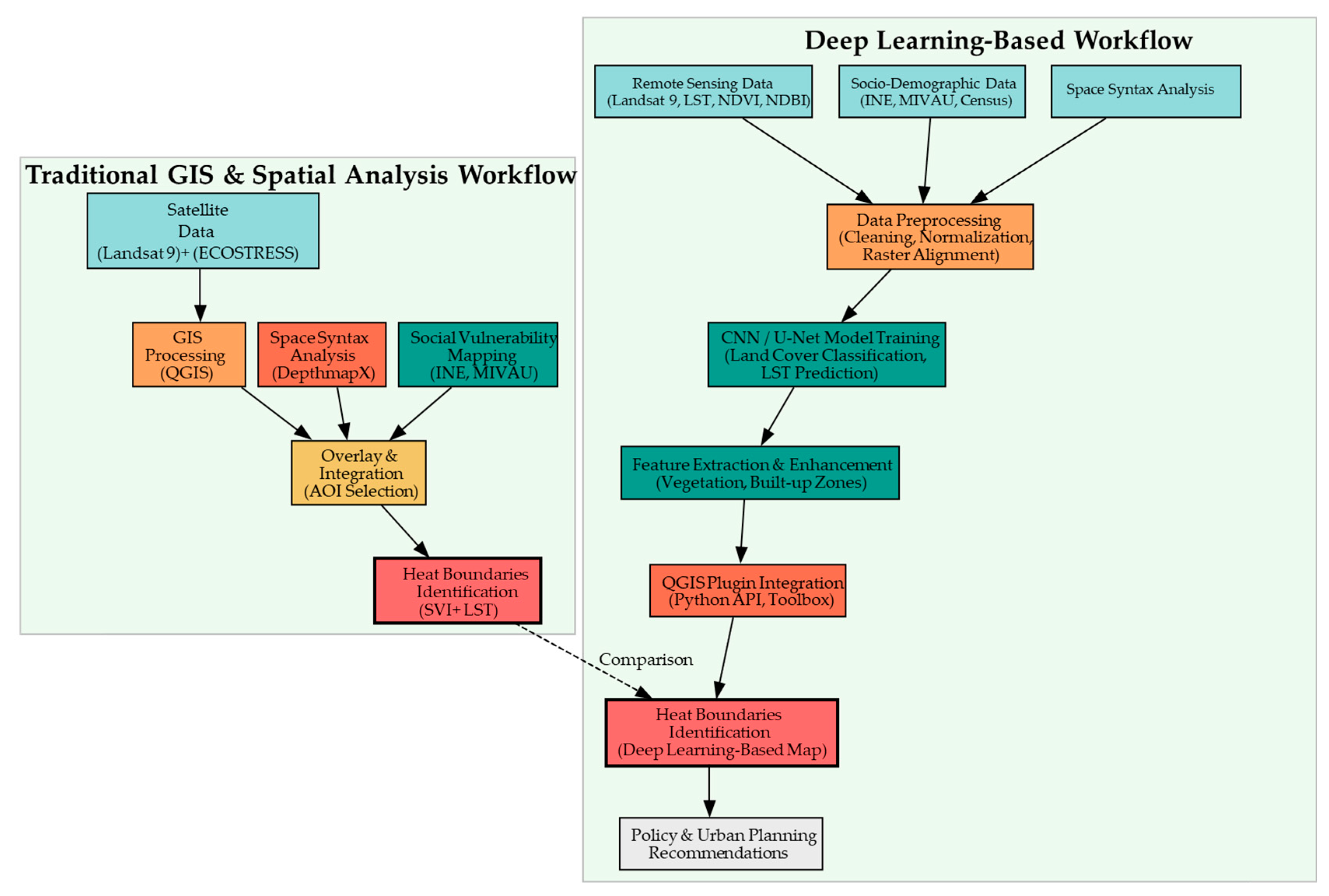
This study employed a multidimensional, multi-scalar analytical approach to assess urban heat vulnerability in Seville, Spain. It integrated remote sensing, spatial configuration analysis via Space Syntax, and socio-demographic vulnerability mapping using GIS-based methods. This methodology operates across both macro-urban and micro-urban scales and spans two distinct summer periods: a heatwave event (26 June 2023) and a non-heatwave summer day (14 July 2024). This comparative temporal framework enables the analysis of both chronic and acute urban heat conditions (Figure 1).
The first phase of the methodology involved mapping Seville’s urban thermal environment using satellite-derived LST, Normalised Difference Vegetation Index (NDVI), and Normalised Difference Built-Up Index (NDBI). These datasets were sourced from Landsat 9 imagery provided by the United States Geological Survey (USGS) [40]. They served as key indicators of diurnal surface heat distribution, vegetation cover, and built-up intensity across the city.
In parallel, a social vulnerability layer was constructed using census data; this layer included socio-economic and demographic attributes, such as income level, housing condition, and population density.
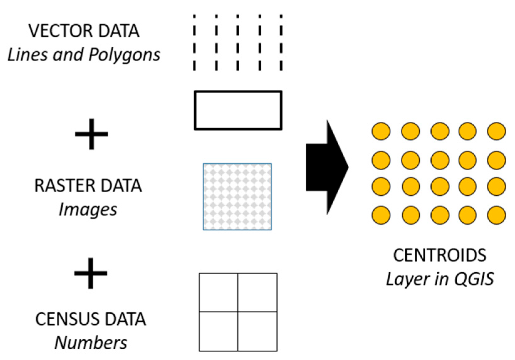
To facilitate integration, all raster and vector datasets were brought into a GIS environment (QGIS); where a centroid-based overlay method was applied. Each urban polygon (e.g., neighbourhood or census block) was assigned thermal and socio-demographic attributes based on the spatial coincidence of centroid points with raster layers (LST, NDVI, NDBI). The choice of Centroids was in favour of random points as it followed a point grid system of 30 X 30 m that ensured covering parts of the neighbourhood and districts’ polygons evenly. The Space Syntax analysis was conducted using all-line axial maps generated with Graph Analysis in DepthmapX software. This spatial configuration analysis using Space Syntax focused on three core syntactic parameters: Connectivity (the number of direct links a street segment has with others), Global Integration (a measure of a segment’s accessibility within the entire street network), and Mean Depth (the average number of steps required to reach all other segments, indicating spatial segregation). Both raster data from remote sensing, socio-demographic data, and vector data from Space Syntax analysis were modelled using QGIS. The main challenge lay in integrating vector data, such as axial line maps and the geometric attributes of polygons and lines, with raster data derived from satellite imagery, alongside statistical indicators, such as vulnerability levels and population density. This was addressed in QGIS using Centroids. A centroid grid was a point layer, Figure 2, generated within QGIS, representing the raster and vector data contained within each polygon [41]. The benefit of using Centroids ensures a systematic and reproducible linkage between vector-based data and raster-based data, and reduces potential bias in the data association process, especially in heterogeneous urban areas.
The methodology consists of two sequential analytical phases. In the first stage, macro-urban scale analysis facilitates the identification of Areas of Interest (AOIs)—specific zones where elevated surface temperatures coincide with high social vulnerability indices. During the second phase, selected AOIs undergo detailed spatial configuration analysis, wherein two contrasting zones are examined at the micro-scale:
  • Zone M: A district with high vulnerability and dense built-up morphology, and highest population density in Seville.
  • Zone W: A river-adjacent zone characterised by traditional urban form.

2.1. Heat Boundary Classification

Following spatial and attribute integration, the methodology includes the classification of Heat Boundaries (HBs). These are defined as urban locations where elevated LST entities act as barriers to adjacent areas of high socio-spatial vulnerability. HB classification is guided by Land Use and Land Cover (LULC) patterns. The classification process enables the delineation of spatially explicit units of urban heat hotspots that can inform future planning and mitigation efforts.
To make decisions for mitigation and recommendations for policymakers, and to evaluate the interrelationships among environmental, morphological, and social variables, a statistical analysis was performed. Both Pearson’s correlation coefficient (r) and Spearman’s rank correlation coefficient (ρ) were calculated. The correlation analysis focuses on assessing:
  • Relationships between LST and vegetation cover (NDVI).
  • Influence of built-up intensity (NDBI) on surface temperatures.
  • Potential associations between spatial configuration parameters (Connectivity, Integration, Mean Depth) and thermal conditions.
  • Interaction between social vulnerability levels and environmental heat indicators.

2.2. Datasets and Variables

Remote sensing data for both scenarios were acquired from the USGS, and Nasa’s ECOSTRESS through the Application for Extracting and Exploring Analysis Ready Samples (AppEEARS) platform [42]. While spatial configuration analyses were conducted using Space Syntax through graph analysis in DepthMapX software. Additional datasets, including demographic and Land Use data, were sourced from the Spanish National Institute of Statistics (INE) [43], Ministry of Housing and Urban Agenda “Ministerio de la Vivienda y Agenda Urbana” (MIVAU) [44], and the Municipality of Seville “Ayuntamiento de Sevilla” [45].
To analyse spatial configuration and variations in street networks at the micro-urban level, Space Syntax indices were employed. These parameters provide quantitative insights into the degree of spatial segregation and integration within each studied urban area, offering a syntactic approach to understanding urban morphology and its effect on urban heat vulnerabilities (Table 1).

2.3. Study Area

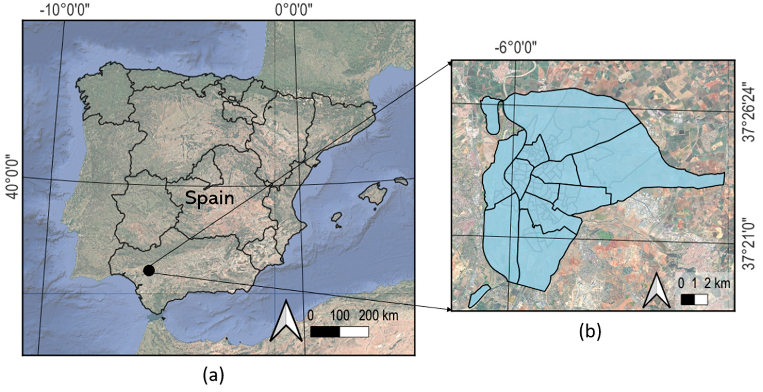
Seville, the capital of Andalusia in southern Spain, is situated at latitude 37°23′10″ N and longitude 5°59′33″ W [46] (Figure 3). Its geographical position and topography make it highly susceptible to extreme heat events and the UHIs effect.
Climate projections indicate that by 2100, temperatures in Seville could rise by approximately 6 °C [46].
Urbanisation in Seville in the last century has shifted population density from the historical city centre to the peripheries and outer neighbourhoods far from the Guadalquivir River. This has resulted in many environmental and social issues and changes in urban heat distribution. A study by Halder et al. [47] reviewed the temporal effects of land alteration on the UHI effect in the city of Seville and found that many changes due to urban expansion and anthropogenic activities have increased LSTs considerably between the years 1991 and 2021; thermal variation increased from (2.21 °C) in 1991 to (3.42 °C) in 2021.
The city’s dense urban development is a result of urbanisation surges, especially the ones that happened between the years 1961 and 1965, which witnessed a population increase of 106,245 people. Consequently, the traditional working-class communities in the old quarter and historic districts, such as Triana, faced displacement due to speculative pressures from the real estate market, relocating to the emerging suburban neighbourhoods on the outskirts and peripheries [48]. Later displacements happened due to gentrification and a decline in the population in the historical areas of Seville caused by over-tourism from the 1990s onward [49]. The extensive unsustainable urbanisation in many areas has caused the intensification of buildings and neighbourhoods, adding more concrete and asphalt, and aggravating the heat problem. Jadraque Gago et al., 2020 [50], reported that the urban areas increased by 37.87% in 2017, compared to the year 1987.

2.3.1. Remote Sensing Data

Understanding the impact of urban dynamics is crucial, and Geographic Information Systems (GISs) tools have become indispensable for urban analytics [51,52,53,54,55].
In recent years, the research has increasingly utilized indices like LST, NDVI, and NDBI. NDVI measures the density of healthy vegetation and helps monitor urban green spaces [56]. It can be used to assess Urban Heat Islands, air quality, and overall urban green infrastructure. NDBI helps detect built-up areas and urban expansion, which is crucial for urban planning and management [57].
The diurnal remote sensing analysis in this study utilizes satellite imagery from Landsat 9, acquired for two distinct temporal scenarios. The first scenario corresponds to the heatwave event on June 26, 2023, and the second to a non-heatwave typical summer day on July 14, 2024, both captured around 11:00 AM GMT.
On the first scenario, the heatwave of 26 June 2023, Seville experienced extreme heat as part of a major heatwave officially named “Yago Sevilla”, under the world’s first system which classifies, and names heatwaves based on health risk and severity [58]. According to AEMET’s municipal-level forecasts [59], the maximum temperature on that day reached approximately 42.00 °C and an average temperature of 32.50 °C, marking one of the peak days of this Category 3 event, the highest level of alert. This made “Yago” the second officially named heatwave in the world, following “Zoe” in 2022, and reflected the growing recognition of heatwaves as critical climate and public health emergencies.
The second scenario corresponds to imagery from Landsat overpass on Seville on 14 July of the year 2024, which was a normal summer day of the same two weeks period between end of June and mid-July. According to AEMET records, the day of 14 July 2024 exhibited normal average temperatures of about 26.00 °C [60].
For diurnal LST, data were acquired using the Thermal Infrared Sensor (TIRS)—specifically bands 10 and 11—and the Operational Land Imager (OLI) using bands 4 and 5. For LST calculations, thermal bands 10 and 11 were used exclusively, while OLI bands were utilised to compute NDVI and NDBI. The inclusion of both temporal scenarios’ diurnal and nocturnal data allows for a comparative assessment of surface temperature conditions under extreme and normal summer scenarios. Both images used in the NDVI analysis were captured during the peak of the dry summer season in Seville, where vegetation activity is typically minimal and stable due to prolonged water stress. Meteorological records confirm similar conditions preceding both image dates, reducing the likelihood of significant phenological variation. NDVI values are thus used to support spatial comparison of vegetation presence across neighbourhoods, rather than to measure seasonal change.
Nocturnal LST data were acquired from the ECOSTRESS sensor using NASA’s AppEEARS platform. Level 2 Land Surface Temperature and Emissivity product (ECO_L2T_LSTE) was selected, and the relevant data layers were requested for each date. To ensure data reliability, only high-quality pixels were retained by applying QC filtering, and LST values were converted from Kelvin to Celsius for interpretability. The platform’s metadata allowed for a confirmation of nighttime acquisition windows, ensuring the images corresponded to post-sunset surface conditions. The resulting data were exported in GeoTIFF format and further processed in QGIS software to extract and compare spatial temperature distributions across different neighbourhoods.
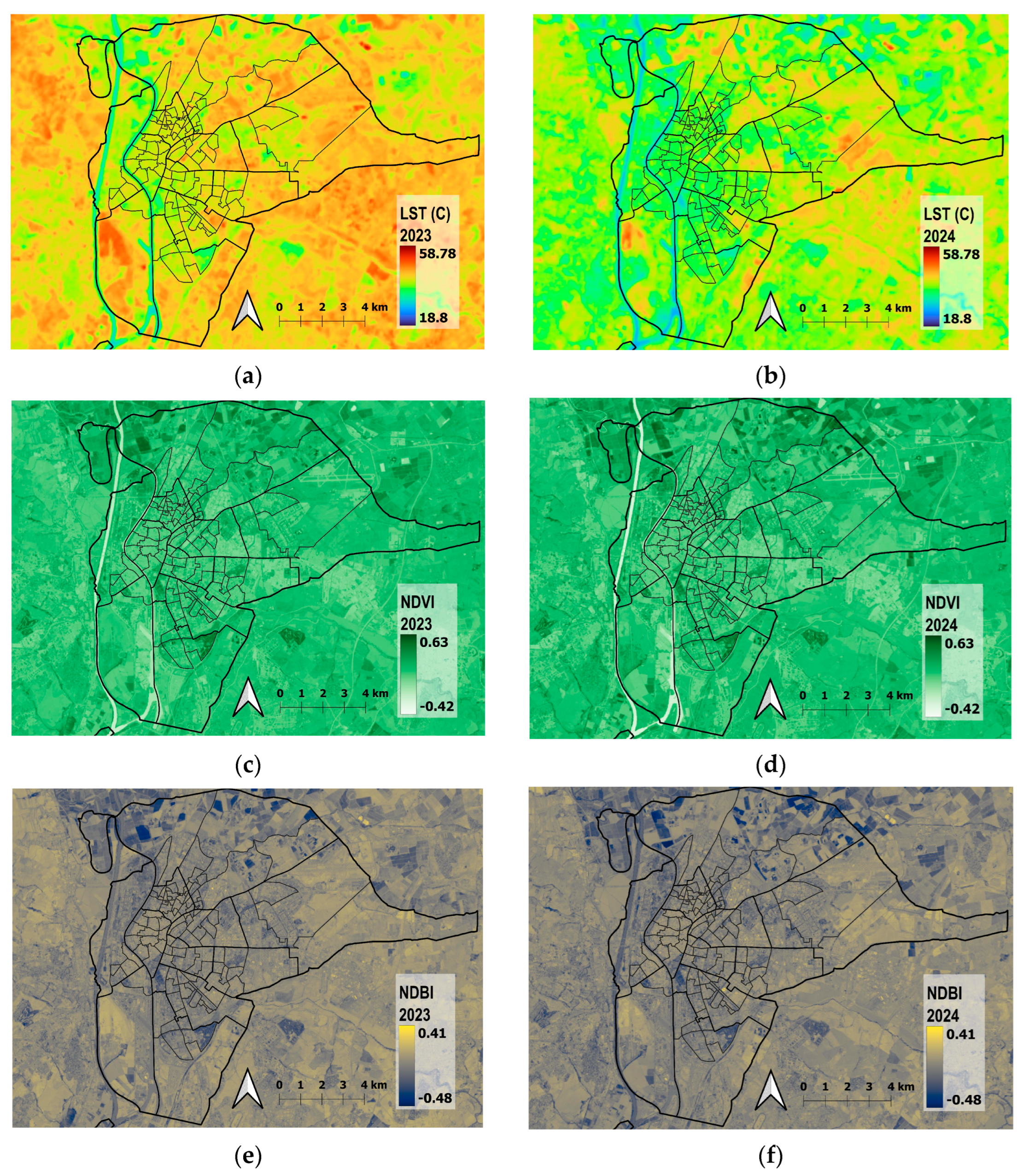
To calculate NDVI, Figure 4c,d, band 5, the Near-Infrared (NIR) and band 4 (Red) from Landsat 9 imagery were utilized. The computation was performed in QGIS using the Raster Calculator, applying Equation (1) [61].
NDVI = (Band 5 − Band 4)/(Band 5 + Band 4)
For NDBI, Figure 4e,f, band 6, the Shortwave Infrared (SWIR 1) and band 5, the Near-Infrared (NIR), from Landsat 9 imagery were utilized. The computation was conducted in QGIS using the Raster Calculator, applying Equation (2) [62].
NDBI = (Band 6 − Band 5)/(Band 6 + Band 5)

2.3.2. Socio-Demographic and Social Vulnerability Data

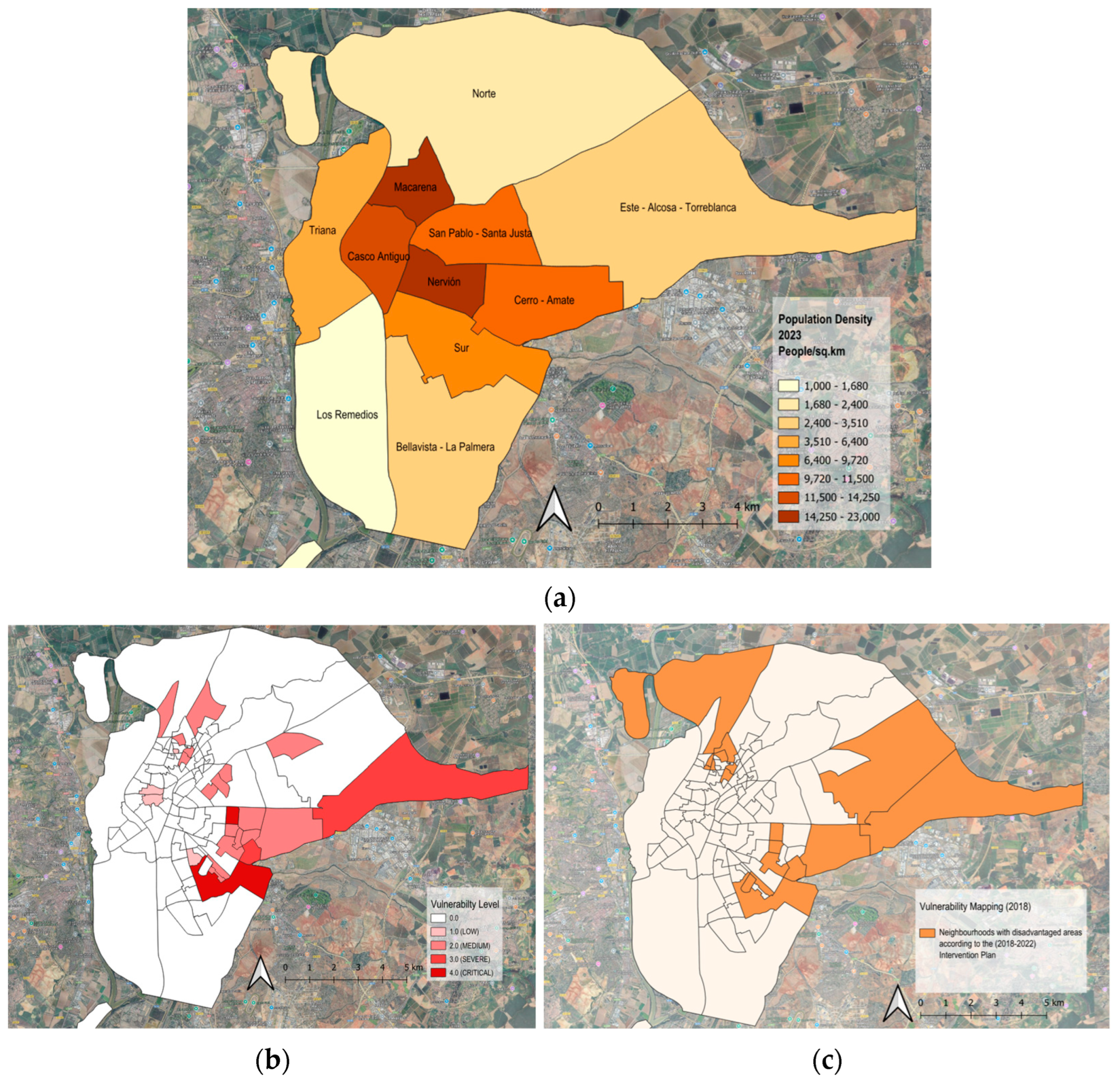
Seville covers an area of 141 square kilometres and is divided into 11 main districts, with a population exceeding 700,000 residents [45]. Urban density varies significantly across the city’s neighbourhoods, as shown in Figure 5a, with the highest population densities found in districts surrounding the historic centre, known as the Casco Antiguo [45]. Among these, the districts of San Pablo-Santa Justa, Cerro-Amate, Nervión, and Macarena exhibit the greatest population concentrations.
Vulnerability mapping in Seville is referenced using governmental census and vulnerability catalogues, which are the main components of the Urban Vulnerability Observatory of the Ministry of Housing and Urban Agenda “Viviendas and Agenda Urbana” [44]. These Catalogues of Vulnerable Neighbourhoods (VNs) in Spain in 1991, 2001, and 2011 examine urban vulnerability in Spanish cities with more than 50,000 inhabitants and provincial capitals. Different criteria were taken into consideration to map vulnerable neighbourhoods, like percentage of old people, children, employment rates, single parents, literacy, and dwelling attributes, etc.
These catalogues classify Seville’s neighbourhoods into four vulnerability levels—providing them a social vulnerability index (SVI) of four levels: Critical (4), Severe (3), Medium (2), and Low (1)—based on the data from 2011 (Figure 5b). This classification serves as a vulnerability weighting factor, which is later used in statistical correlations with other numerical variables.
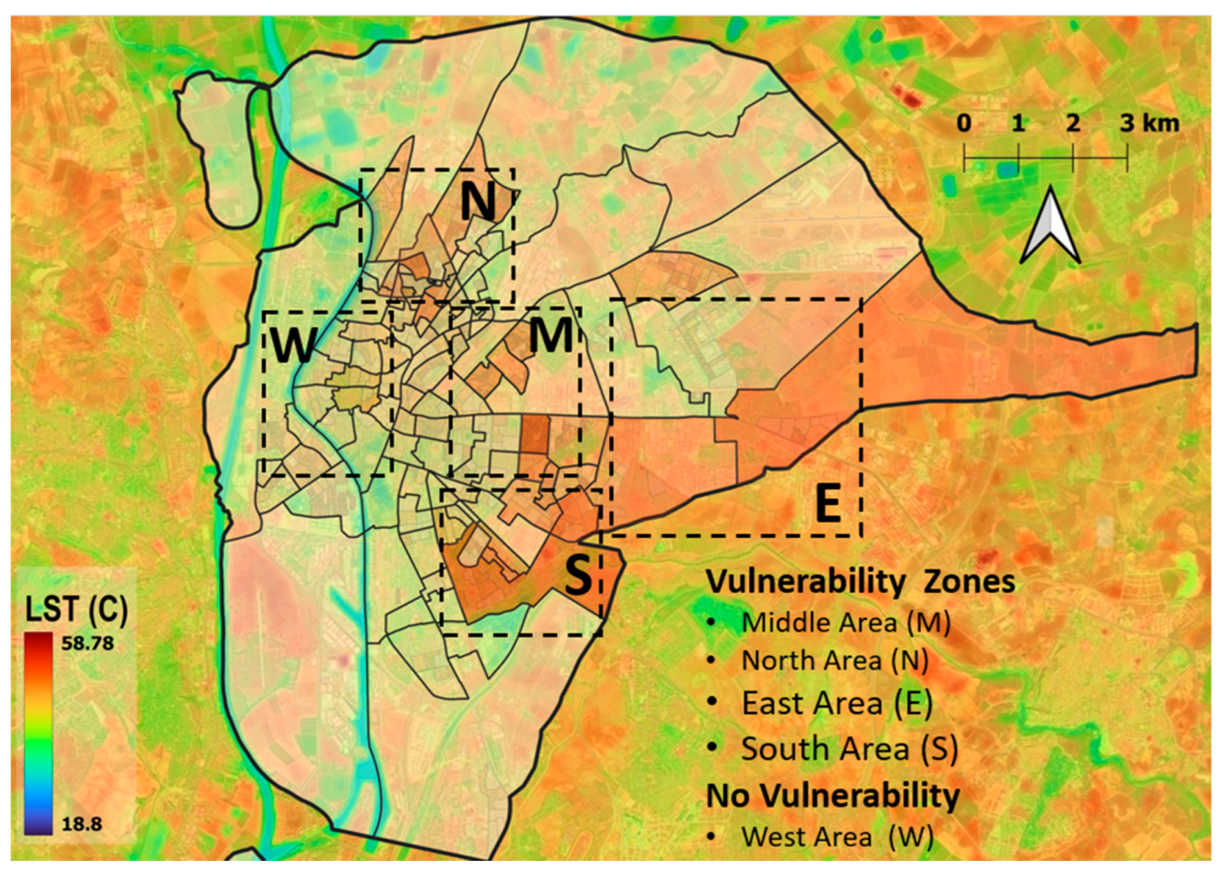
Another essential data source for understanding urban vulnerability is the Local Plan for the Intervention in Disadvantaged Areas of Seville (2018–2022), published by the Seville City Council in 2018 [63]. This plan identifies disadvantaged neighbourhoods, defined by high unemployment rates and a concentration of socio-economic risk factors. In addition. Overlaying all these social census layers in QGIS into a single composite map is essential for identifying patterns of urban vulnerability in relation to urban heat. This integrative mapping process also helps guide the selection of specific Areas of Interest (AOIs) [64] for further in-depth analysis. For micro-scale mapping, the combined layers of LST and social vulnerability were further examined to identify Land Uses and neighbourhood boundaries, as illustrated in Figure 6. The process employed layers multiple social census datasets—including population density, vulnerability levels (2011), disadvantaged areas (2018), and (LST) maps from June 26, 2023 and July 14, 2024—to delineate the final focused micro-urban study areas. This spatial analysis highlights four key zones where social vulnerability overlaps with elevated LST values: the central middle Zone (M), eastern Zone (E), southern Zone (S), and northern Zone (N). In contrast, the western area, Zone (W), located along the Guadalquivir River, exhibits cooler urban temperatures and no significant signs of social vulnerability.

2.3.3. Spatial Configuration Using Space Syntax

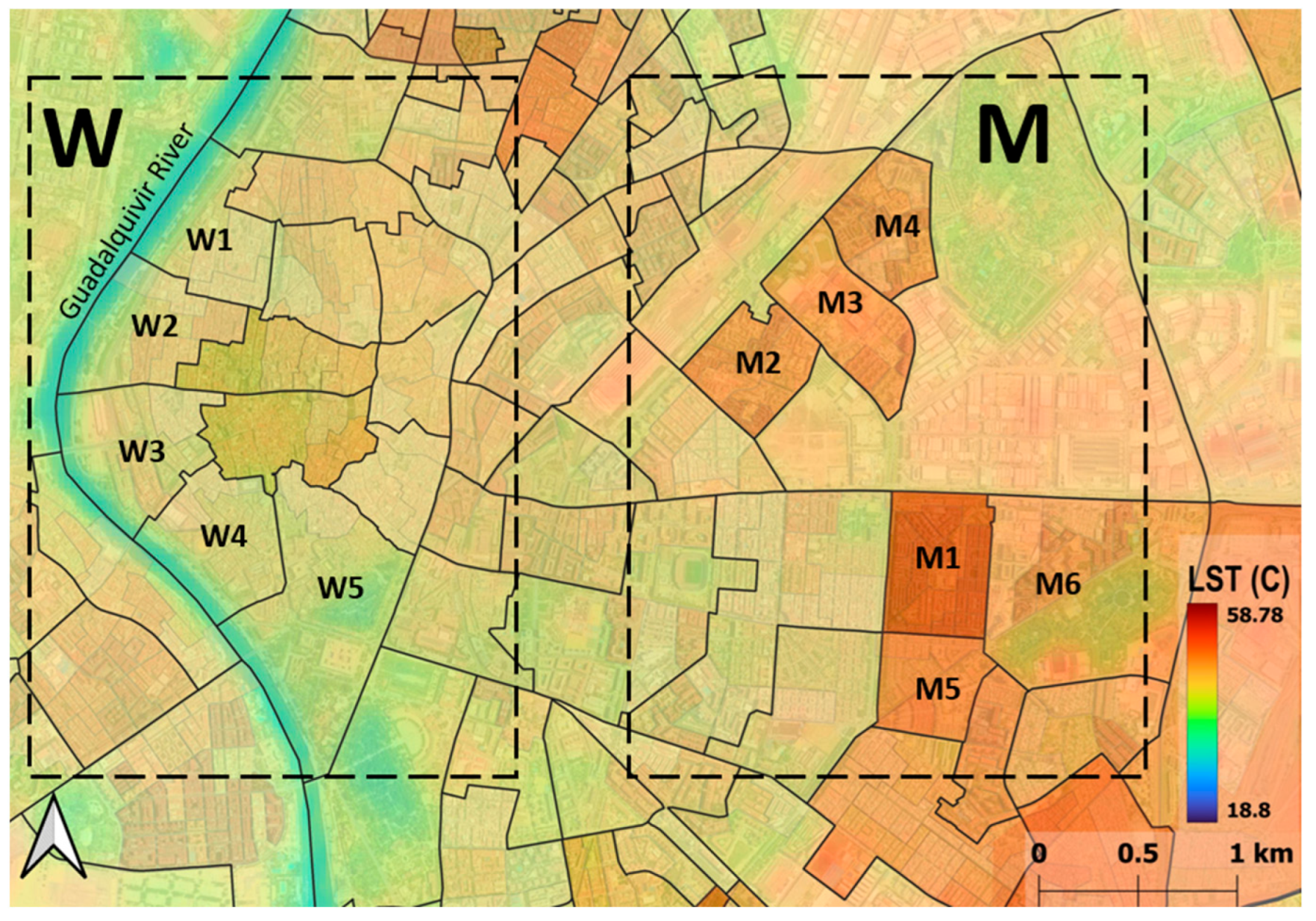
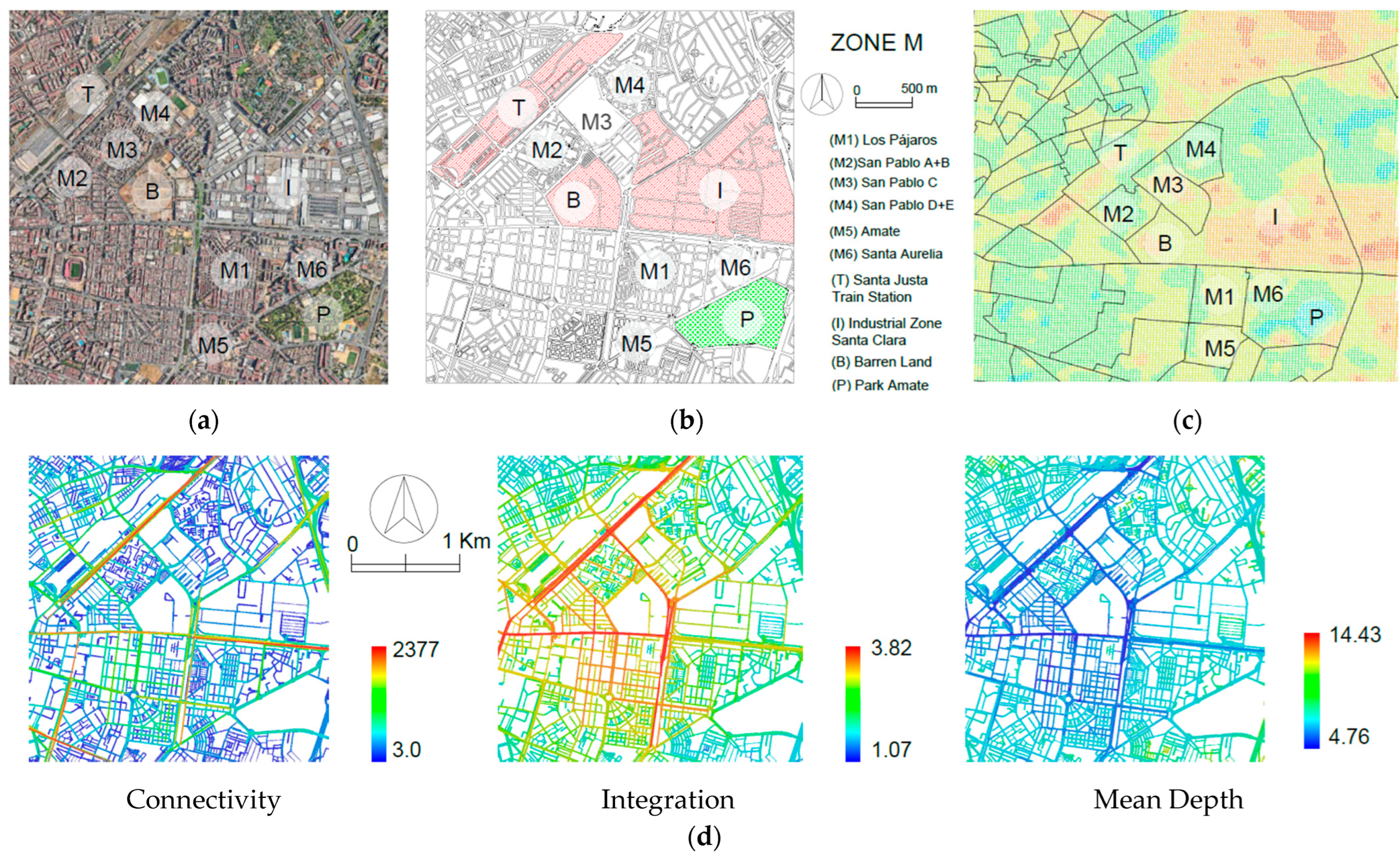
The spatial analysis began with the identification and selection of two distinct AOIs, a process informed by the data layering process presented in Figure 6. This process identified zones that combine varying levels of heat exposure and social vulnerability. Based on this analysis, two distinct focused AOIs were selected, each covering approximately 7.25 km2. The first Area of Interest (AOI), Figure 7, referred to as “Zone M”, includes the neighbourhoods of Los Pájaros (M1), San Pablo A + B (M2), San Pablo C (M3), and San Pablo D + E (M4). This zone is characterized by both high social vulnerability and elevated surface temperatures. Notably, Los Pájaros (M1) ranks among the most disadvantaged neighbourhoods in Spain, according to the Spanish National Institute of Statistics [43].
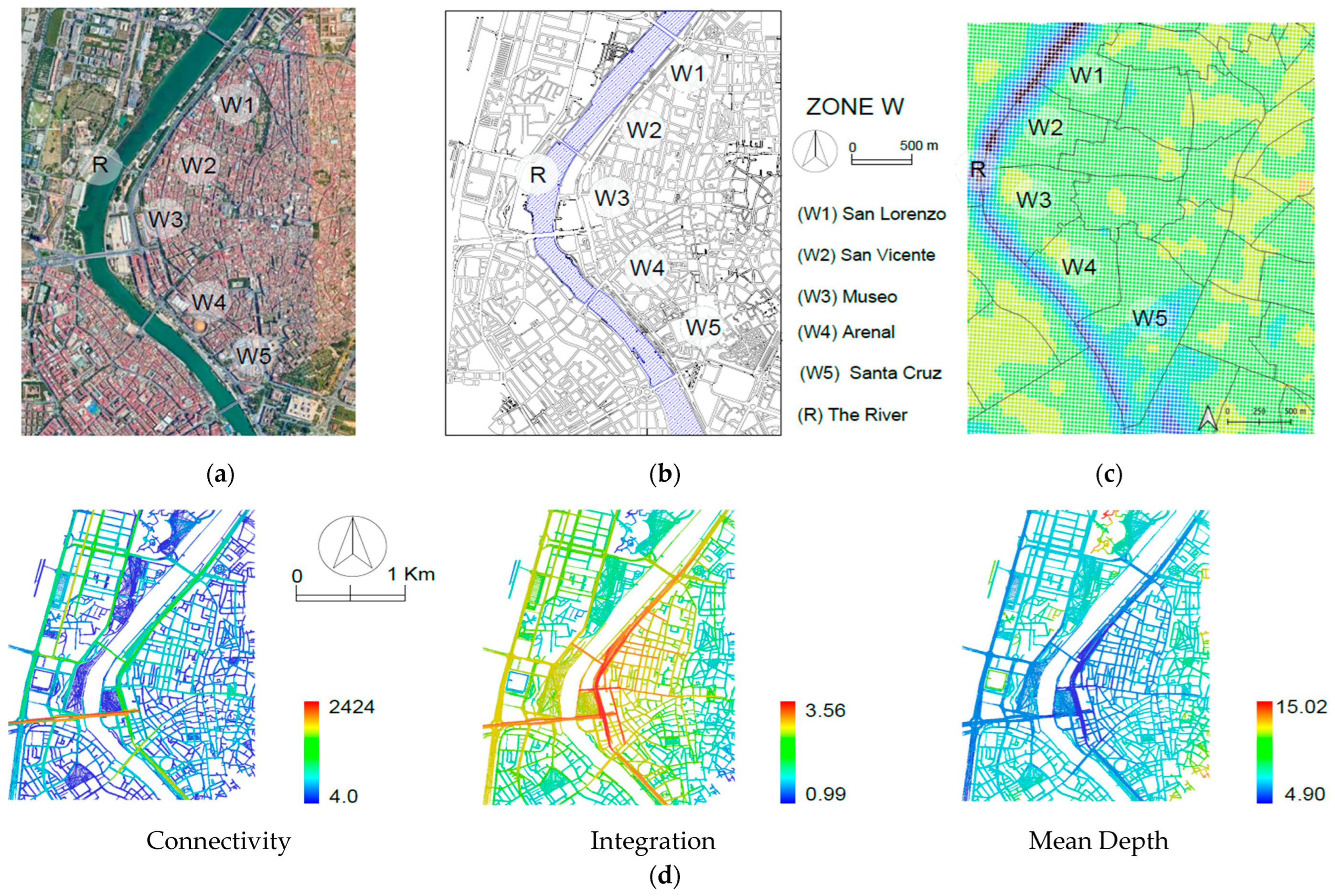
The second AOI, “Zone W”, Figure 7, represents a more affluent and low-vulnerability area, with minimal social risk factors and generally better environmental conditions. Its proximity to the Guadalquivir River contributes to a noticeable cooling effect.
Both neighbourhoods share high population densities, with contrasting urban fabric characteristics. While Zone M is considered a low-income area, Zone W is more affluent in terms of social and economic value. For each AOI, the analysis focuses on Connectivity, Integration, and Mean Depth, specifically along the main streets in each neighbourhood; the main streets are usually the street with highest Connectivity levels measured by Space Syntax. The objective is to detect potential patterns of spatial segregation (lower Connectivity, less Integration, and higher Mean Depth) and hence added urban vulnerability.

3. Results

3.1. Macro-Urban Data Results

Macro-urban data analysis results represent two contrasting climatic conditions—a heatwave event in June 2023, Table 2, and a normal summer day in July 2024, Table 3. The results reflect the spatial–temporal variability in LST, NDVI, and NDBI across different urban zones (M, N, S, E, W, peripheries), offering insights into how urban morphology and social vulnerability intersect with urban heat vulnerability at the neighbourhood level during two heatwave diurnal scenarios. ANOVA testing revealed a statistically significant difference in mean Land Surface Temperature (LST) among urban zones in Seville during both scenarios. The F-ratio is 45.98 and the p-value is less than 0.00001, indicating that the result is significant at the p < 0.05 level. This suggests that the variation in LSTs across different neighbourhoods and zones reflects real differences in thermal conditions throughout the city.

3.1.1. Highest Diurnal LST Values Are in the Peripheries

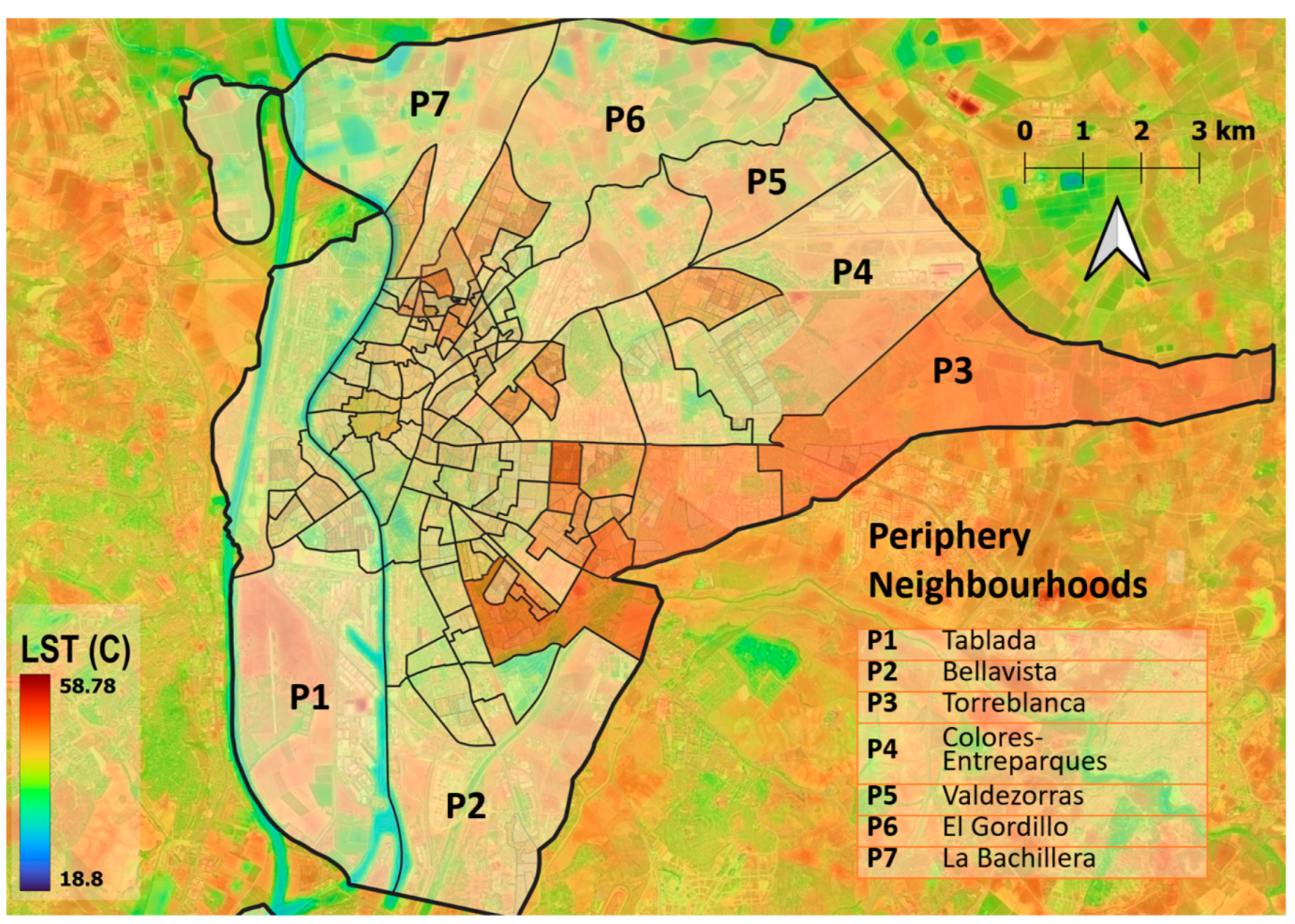
During both heatwave and non-heatwave conditions, peripheral zones, Figure 8, recorded the highest LST values across the city during the day. In the 2023 heatwave, Las Letanías-Paz y Amistad (S2) recorded the peak LST at 53.99 °C, followed closely by Tablada (P1) at 53.99 °C and Colores-Entreparques (P4) at 53.10 °C. These areas are characterized by extensive impervious and barren land, minimal vegetation, and critical levels of social vulnerability, intensifying heat retention.
In the non-heatwave scenario (2024), while diurnal LSTs were generally lower, Tablada (P1) still reached a maximum of 50.81 °C, Torreblanca (P3) reached 50.10 °C, and Colores-Entreparques (P4) a peripheral neighbourhood in the northeast, Figure 8, where the Seville airport is located, recorded a maximum LST of 49.62 °C. The airport complex, characterized by impervious surfaces, extensive barren land, and minimal vegetation cover, contributes to aggravated urban heat, as impervious surfaces increase urban heat [65]. These high LST values correspond with very low NDVI readings in the urban peripheries for 2023 and 2024 (0.14 and 0.18, respectively), alongside elevated NDBI values with averages of 0.01 and 0.02 for the same periods. This pattern confirms that sparse vegetation contributes to heat intensification, consistent with the previous research showing that barren urban peripheries experience extreme surface heating during summer months [66].

3.1.2. Diurnal LST Variations Between Different Zones

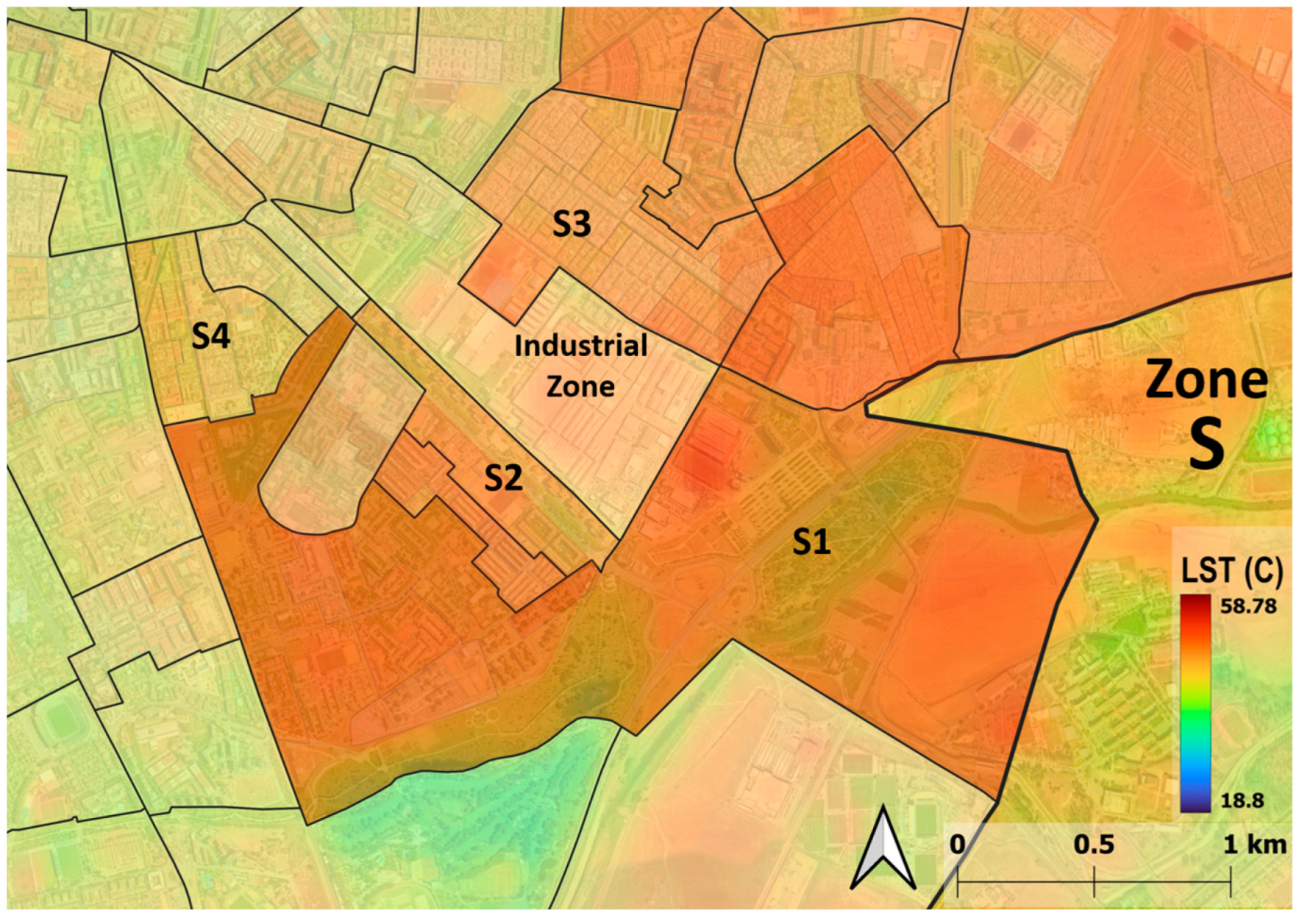
Thermal disparities across Seville’s zones reveal that less-advantaged neighbourhoods tend to experience higher temperatures. In the heatwave scenario, Polígono Sur (S1), one of the most socio-economically vulnerable neighbourhoods, SVI = 4, adjacent to the industrial zone of “El Juncal-Híspalis”, Figure 9, recorded a maximum diurnal LST of 51.21 °C and an average of 42.97 °C.
In comparison, Zone W, a more advantaged zone, located along the Guadalquivir River and featuring traditional urban morphology with narrower streets and shaded walkways, had significantly lower temperatures. For example, San Lorenzo (W1) recorded a maximum LST of 42.69 °C and an average of 39.31 °C in the heatwave scenario of 2023, and even lower values during 2024, a maximum LST of 38.57 °C and an average of 36.00 °C, illustrating the river’s cooling influence. Overall, during the heatwave scenario on June 26, 2023, temperatures were notably higher across all zones. The average LST across Zone W was 36.74 °C, significantly lower than 42.49 °C in Zone M (a difference of 5.75 °C) and 44.02 °C in the peripheries (a difference of 7.28 °C).
For the non-heatwave scenario of 2024, the average diurnal LST across Zone W (W1–W5) was 36.08 °C, compared to 38.63 °C in Zone M (a difference of 2.55 °C) and 39.85 °C in the peripheries (a difference of 3.77 °C from Zone W).
These consistent thermal disparities across both time periods emphasise the protective influence of river-adjacent urban morphology in Zone W, where narrower streets, higher vegetation coverage, and access to water bodies contribute to enhanced thermal regulation, especially under extreme heat events.

3.1.3. NDVI and NDBI Between Zones

Vegetation cover, as measured by the NDVI, and built-up density, indicated by the NDBI, both exhibit clear spatial contrasts that align with thermal patterns.
NDVI analysis reveals contrasting vegetation patterns between scenarios. During the 2023 heatwave, mean NDVI values were generally low across all zones, with Zone W averaging 0.10 and peripheries showing slightly higher values at 0.16. The 2024 non-heatwave scenario exhibited improved vegetation conditions, with Zone W maintaining similar low values (0.10) while peripheries showed significantly enhanced vegetation cover (0.18). This suggests that normal climatic conditions may support better vegetation health, particularly in peripheral urban areas. Zones M, N, and S demonstrated relatively stable vegetation patterns between scenarios, while Zones E showed slight decreases in vegetation cover during the normal summer period.
During the 2023 heatwave, peripheries exhibited positive NDBI values (0.012), suggesting relatively higher built-up density, while most urban zones showed negative values, indicating more natural surfaces. The 2024 non-heatwave scenario revealed a notable shift, with peripheries displaying negative NDBI values (−0.02), suggesting reduced built-up intensity or improved surface permeability. Zone S showed increased built-up characteristics in 2024 (0.01) compared to 2023 (0.00), while Zones M and N demonstrated decreased built-up intensity during the normal summer period.

3.2. Nighttime LST Data

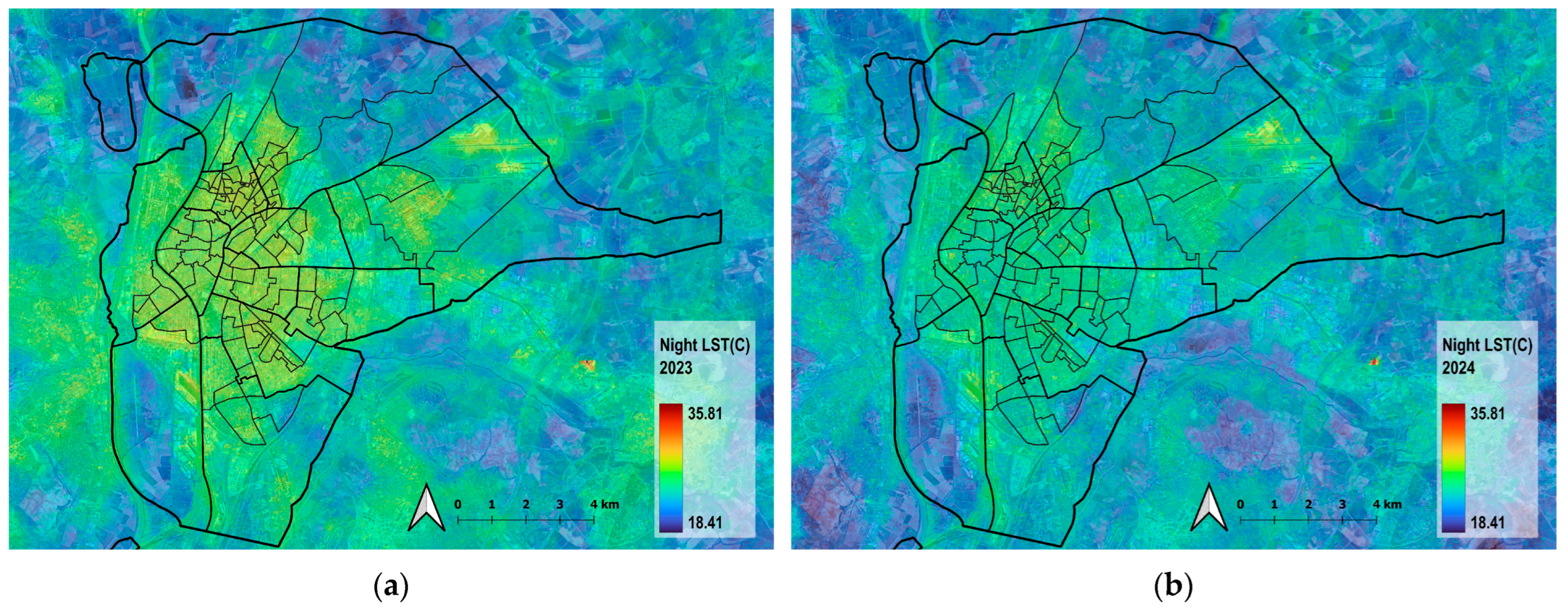
To provide additional insights into nocturnal thermal patterns, ECOSTRESS satellite data were utilized, corresponding to the nighttime overpasses of June 26, 2023 (during the heatwave) and July 14, 2024 (during the non-heatwave scenario) (Figure 10). Both nighttime datasets were acquired at 3:00 AM GMT. They complement the Landsat 9 data acquired on the same dates during the day at 11:00 AM GMT. The data were acquired from Nasa’s ECOSTRESS through the AppEEARS platform.
Across both scenarios, nighttime LST, Table 4, follows a broadly similar spatial pattern; with Zones N, M, and S having the highest LSTs on average, followed by Zone W, Zone E, and the peripheries being the coolest, contrary to diurnal data, where highest LSTs are in the peripheries.
All zones experienced notably lower average nighttime Land Surface Temperatures in 2024 compared to 2023, reflecting the difference between the heatwave and normal summer conditions. The largest absolute difference was observed in Zone S (1.84 °C cooler in 2024), and the smallest in the peripheries (0.30 °C cooler in 2024). Zone S was the warmest during the 2024 non-heatwave night (24.71 °C). Peripheries remained the coolest zone in both scenarios.
A comparison of nighttime Land Surface Temperatures between Zone M and Zone W reveals distinct thermal patterns across both climatic scenarios. During the 2023 heatwave night, Zone M exhibited a slightly higher average LST of 26.82 °C compared to Zone W’s average of 26.71 °C, indicating that the central urban area (Zone M) retained more heat than the western zone (Zone W) during the extreme heat event. This pattern changed under normal summer conditions in 2024, where Zone M again showed slightly lower nighttime temperatures (25.08 °C) compared to Zone W (25.17 °C). This difference indicates that urban zones characterized by a high population density, heavy traffic, and extensive built-up infrastructure exhibit elevated nighttime LSTs compared to peripheral areas and vacant lots; nighttime LST patterns are complex [67] and are mostly affected by urban density [68].

3.3. Micro-Urban Spatial Analysis Results

For the spatial configuration of Zone M, Figure 11, the data for key roads, such as “Av. de Andalucía” (running East to West) and “Calle Clemente Hidalgo” (running North to South), were analysed. At the intersection of these two roads is Los Pájaros (M1), one of the most impoverished and vulnerable areas in Spain. Additionally, “Av. de Kansas City” separates the three vulnerable neighbourhoods of (M2, M3, M4) from Santa Justa, Seville’s main train station.
Axial analysis was also conducted on the street network for Zone W, located along the Guadalquivir River, which traditionally borders the old city centre (Casco Antiguo). Many neighbourhoods near the river benefit from low LST values. These neighbourhoods are shown in Figure 12, including San Lorenzo (W1), San Vicente (W2), Museo (W3), Arenal (W4), Santa Cruz (W5), among others. The street “Calle Torneo”, which runs parallel to the river, forms a boundary to these neighbourhood.
Table 5 highlights notable variations in diurnal and nocturnal LSTs across street networks in Zones M and W under both heatwave and non-heatwave conditions. In Zone M, which is a less-advantaged area, has the highest population density in the city, and is characterized by limited greenery; key streets such as Avenida de Andalucía consistently recorded the highest LST values across both heatwave (2023) and non-heatwave (2024) scenarios, in both daytime and nighttime conditions. During the 2023 heatwave, Avenida de Andalucía reached daytime average LSTs of 43.53 °C (max: 45.30 °C) and nighttime LSTs of 25.77 °C (max: 27.13 °C). Even during the milder 2024 summer, the street recorded average daytime LSTs of 40.04 °C and nighttime LSTs of 24.52 °C, suggesting persistent nocturnal heat retention.
In contrast, Zone W, bordering the Guadalquivir River and composed of neighbourhoods such as San Vicente (W2) and Museo (W3), demonstrated significantly lower LSTs, particularly at night. In 2023, streets like Calle Reyes Católicos and Calle Torneo showed average nighttime LSTs around 26.60 °C, while in 2024, the values dropped further to a range of 25.40–25.60 °C. The daytime LSTs also reduced from 40.09 °C to 35.93 °C, showing a strong cooling trend under non-extreme conditions.

4. Discussion

4.1. Correlation and Regression

4.1.1. Macro-Urban Spatial Analysis Correlations

Correlation analyses were conducted for the resulting remote sensing data in Table 2 and Table 3, for both scenarios of heatwave and non-heatwave, to examine relationships among key variables in different zones for both daytime and nighttime LSTs.
Both Pearson’s correlation coefficient (r) and Spearman’s rank correlation coefficient (ρ) were employed to analyse relationships between variables, ensuring a comprehensive assessment of both linear and monotonic associations. Pearson’s r quantifies linear relationships under normality assumptions, while Spearman’s ρ is a rank-based, non-parametric measure that captures monotonic trends, making it robust against non-normality and outliers. Using both allows for a comparative analysis, validation of assumptions, and detection of non-linear patterns, ensuring a more nuanced interpretation of correlation structures [69].
As shown in Table 6, the results for the different AOIs (M, W, E, S, P) reveal a complex interaction between LST, vegetation cover (NDVI), and built-up intensity (NDBI). Correlation analyses were conducted under two temporal scenarios: a heatwave event on 26 June 2023 and a non-heatwave day on 14 July 2024. These dual scenarios provide insights into how urban form, vegetation, and socio-demographic vulnerability influence thermal patterns under both summer conditions for daytime and nighttime LSTs.
During the 2023 heatwave, vegetation cover (NDVI Average) exhibited a moderate positive correlation with the daytime average LST (Pearson’s r = 0.43, p = 0.02; Spearman’s ρ = 0.35, p = 0.05), a counterintuitive finding that suggests vegetation in Seville’s vulnerable zones may be sparse, fragmented, or insufficiently dense to provide significant daytime cooling.
In the 2024 non-heatwave scenario, the NDVI maintained a significant but slightly weaker correlation with daytime average LST (Pearson’s r = 0.38, p = 0.03), while Spearman’s ρ increased to 0.43 (p = 0.01), indicating that under milder conditions, even modest vegetation can help reduce thermal stress. This reinforces the importance of green infrastructure, but highlights that its impact is not uniformly beneficial unless vegetation is sufficiently dense, continuous, and strategically placed.
Built-up intensity, measured by NDBI Average, consistently showed the strongest and most robust correlation with average LST across both years. In 2023, the correlation with LST was significant (Pearson’s r = 0.43, p = 0.01; Spearman’s ρ = 0.57, p = 0.00), indicating that more urbanized zones, particularly those with high impervious surface cover, accumulate and radiate more heat during the day.
Although in 2024 the Pearson’s correlation weakened (Pearson’s r = 0.28, p = 0.13), the trend remained consistent, reflecting the persistent influence of urban morphology on thermal conditions. Spearman’s correlation also dropped (ρ = 0.28, p = 0.12), suggesting that under non-extreme heat conditions, urban form continues to shape temperature patterns but with reduced statistical strength. This may indicate that urban material properties and layout primarily govern heat accumulation during heatwaves, while their influence is partially diminished in regular summer weather.
The relationship between social vulnerability (SVI) and daytime LST was moderate and statistically significant in 2023 (Pearson’s r = 0.35, p = 0.05), but the Spearman’s result was not significant (ρ = 0.11, p = 0.54), pointing to a non-linear and non-monotonic relationship. Vulnerable populations are likely concentrated in areas of higher built-up density and lower vegetation, but this correlation alone cannot capture the spatial variability and complexity of urban form or human adaptation strategies.
In the non-heatwave 2024 scenario, the relationship between the SVI and average LST weakened further (Pearson’s r = 0.27, p = 0.14; Spearman’s ρ = 0.23, p = 0.21), losing statistical significance. This suggests that the thermal disadvantage of socially vulnerable groups becomes more pronounced under extreme heat events.

4.1.2. Micro-Urban Spatial Analysis Correlations

At the micro-urban scale, spatial syntax variables—Connectivity, Global Integration, and Mean Depth—were examined to understand how street network configuration correlates with diurnal surface temperature patterns in both heatwave and non-heatwave contexts. These syntactic attributes are crucial for assessing how the form and accessibility of urban spaces modulate thermal exposure at the street level.
In the 2023 heatwave scenario, Table 7, Connectivity and Global Integration show weak and non-significant correlations with average daytime LST (Pearson’s r = 0.18, p = 0.62; r = –0.32, p = 0.36, respectively), indicating the limited influence of street network openness or accessibility on Land Surface Temperature. Similar findings were obtained for Spearman’s ρ, reinforcing the non-linear and weak nature of these associations.
However, Mean Depth, which reflects the relative isolation of a space within the network, demonstrated a moderate positive correlation with diurnal average LST (Pearson’s r = 0.49, p = 0.15; Spearman’s ρ = 0.49, p = 0.15), implying that deeper and less integrated street segments may trap more heat, potentially due to restricted airflow and shading limitations—linking vulnerability to heat with segregated streets and zones of the urban fabric configuration.
The relationship between social vulnerability (SVI) and diurnal average LST was statistically significant in both Pearson’s and Spearman’s tests (Pearson’s r = 0.70, p = 0.03; Spearman’s ρ = 0.77, p = 0.01). This confirms that during heatwave conditions, vulnerable neighbourhoods are disproportionately affected by elevated surface temperatures, highlighting a socio-spatial disparity in urban heat exposure.
In the non-heatwave scenario (2024), these trends were largely consistent. Connectivity and Global Integration remained weakly correlated with average LST (Pearson’s r = 0.20 and –0.29, respectively), and neither correlation reached statistical significance. Mean Depth continued to show a moderate positive correlation (Pearson’s r = 0.47, p = 0.17), reinforcing the role of spatial enclosure and higher LSTs in the deeper streets of the network. Notably, the correlation between SVI and average LST remained significant in 2024 (Pearson’s r = 0.72, p = 0.02; Spearman’s ρ = 0.77, p = 0.01), suggesting that vulnerable zones are consistently exposed to higher temperatures even outside heatwave conditions.
This indicates a persistent spatial inequality in thermal exposure at the micro-urban scale. The results demonstrate that syntactic spatial configuration variables alone are insufficient for predicting temperature distribution patterns. However, the spatial depth of streets (Mean Depth) and social vulnerability (social vulnerability index—SVI) emerge as significant determinants of micro-urban heat dynamics, particularly during heatwave conditions. This relationship is exemplified by the substantial thermal disparity observed between socio-spatially distinct zones: vulnerable Zone M streets exhibited an average diurnal LST of 42.67 °C during the heatwave, while less vulnerable Zone W streets maintained a considerably cooler average of 39.81 °C. This pronounced temperature differential along socio-spatial gradients underscores the critical importance of incorporating spatial configuration analysis to understand and address urban heat vulnerability patterns.

4.2. Mapping Heat Boundaries (HBs)

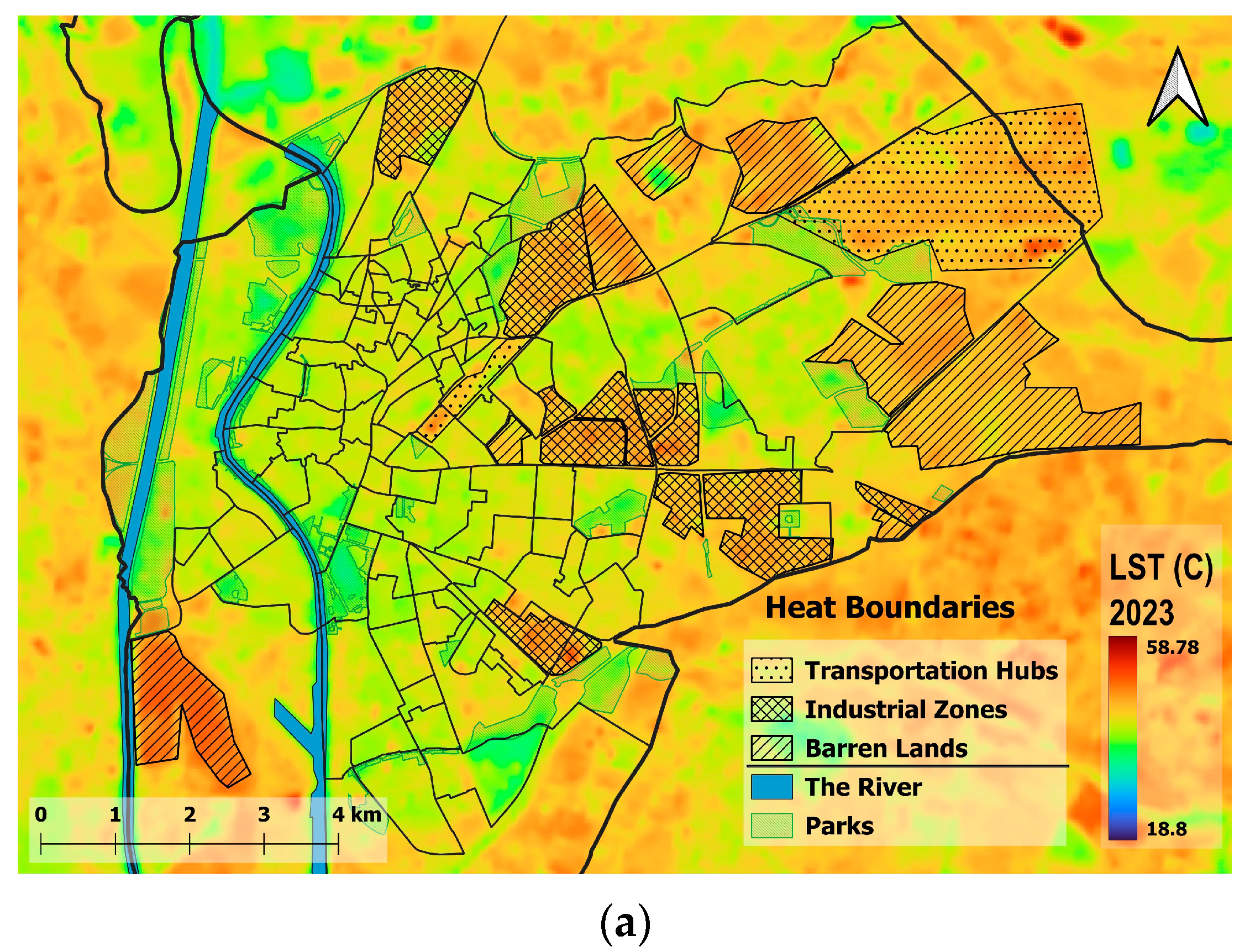
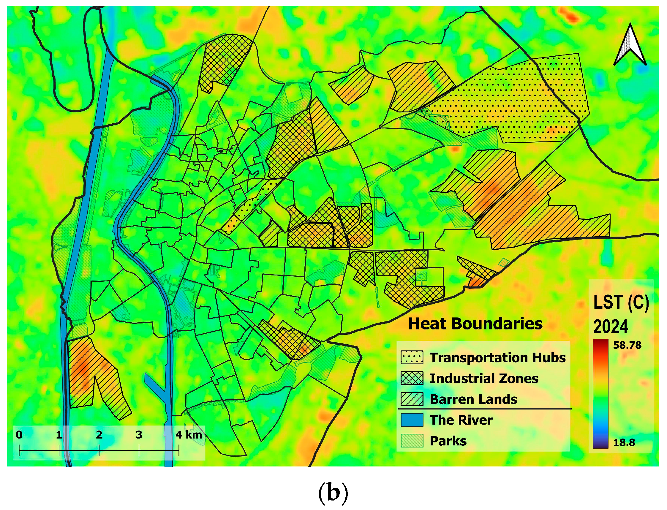
The analysis of macro-urban thermal patterns in Seville under two temporal scenarios, the heatwave event on 26 June 2023 and a non-heatwave day on 14 July 2024, demonstrates a consistent spatial structure in urban heat distribution across the city. As visualised in Figure 13, the delineation of Heat Boundaries (HBs) during the daytime remains largely unchanged between both scenarios, indicating their reliability and stability as spatial indicators of urban heat accumulation.
HBs are spatial entities identified as persistent urban heat hotspots, revealed through the integration of satellite-derived remote sensing data and macro-urban spatial analysis. These boundaries were classified into three primary Land Use/Land Cover (LULC) categories in Seville:
  • Barren lands (accounting for about 42% of HBs).
  • Industrial zones (accounting for about 30%).
  • Transportation hubs, such as Santa Justa Train Station and Seville Airport (28%).
Together, these zones account for approximately 17% of Seville’s urban area, with barren lands emerging as the dominant contributor to elevated diurnal LST values. This consistent classification across both scenarios supports their relevance and robustness in representing enduring urban heat hotspots, regardless of short-term climatic fluctuations.
Despite the temperature variability between the two scenarios, the spatial distribution and allocation of HBs remain almost the same, as shown in both heatwave and non-heatwave scenarios in Figure 13a,b. This suggests that HBs are not just a result of temporary heat events, but are structurally embedded in the urban landscape, shaped by Land Use intensity, material properties, and spatial exposure.
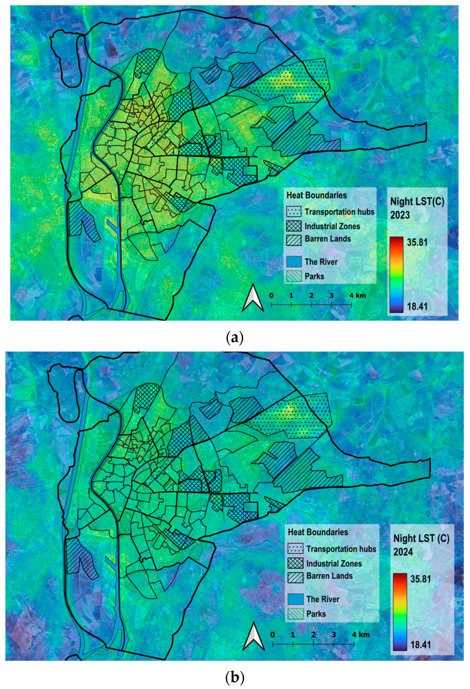
In the analysis of HBs with reference to nighttime LSTs, Figure 14a illustrates the heatwave scenario and Figure 14b the non-heatwave scenario. The delineation of hotspots remains largely consistent for transportation hubs across both scenarios, though less consistent for industrial zones between daytime and nighttime conditions. Conversely, barren lands on the peripheries of the city exhibit almost opposite patterns, tending to show lower LSTs during nighttime conditions. This fluctuation of LSTs between day and night requires further analysis that incorporates additional environmental, phenological, and spatial parameters. One consistent finding is that urban areas with a high population concentration remain LST hotspots across all scenarios, highlighting the critical need for resilience strategies in high-density urban areas, particularly those in socially disadvantaged neighbourhoods.
The selection of these areas as Heat Boundaries in our research is fundamentally driven by their critical role in revealing patterns of thermal inequity and spatial segregation. This study’s delineated HBs are strategically located adjacent to socio-economically vulnerable neighbourhoods, thereby reinforcing and highlighting existing patterns of thermal disparity across the urban landscape.
At the macro-urban scale, our analysis demonstrates significant temperature variations between vulnerable neighbourhoods situated at varying distances from the Guadalquivir River, a major water body that serves as a crucial cooling infrastructure. This spatial relationship between socio-economic vulnerability and proximity to natural cooling features represents a core research objective—understanding how urban morphology and environmental amenities intersect with social equity in determining heat exposure.
In contrast to HBs, Cooling Boundaries (CBs), particularly the Guadalquivir River and extensive urban parks and green areas, constitute approximately 18% of Seville’s total area and function as natural Urban Cool Islands (UCIs). These water and green surfaces create essential cooling corridors that significantly reduce LST values in their immediate vicinity [70]. The stark thermal contrast between HBs and CBs, especially for neighbourhoods directly bordering these natural cooling features versus those isolated from them, underscores the importance of these areas in achieving our research goals of identifying and understanding the spatial dynamics of urban heat vulnerability. This juxtaposition of hot and cool boundaries provides crucial insights into how urban planning and environmental justice intersect in the context of climate resilience.

4.3. Study Limitations

This study contributes to the advancement of urban heat vulnerability research by integrating remote sensing data, Space Syntax analysis, and social vulnerability metrics within a comprehensive multidimensional framework. The findings highlight the value of such integrative approaches in informing climate-adaptive urban planning and enabling targeted policy interventions. However, several limitations must be acknowledged.
A key limitation lies in the temporal scope of the analysis, which only compares two distinct temporal scenarios representing distinct summer conditions for both diurnal and nocturnal LSTs. While sufficient for this study’s aim of examining urban heat exposure and vulnerability during peak thermal stress, they do not capture the broader temporal variability of urban heat patterns, which fluctuate across diurnal, weekly, and seasonal scales. Future research should incorporate long-term remote sensing archives or continuous in situ monitoring to better account for this variability and strengthen the robustness of conclusions.
Another constraint concerns the spatial and temporal characteristics of the remote sensing data employed. Landsat 9 thermal imagery offers superior spatial resolution—30 m for optical bands and 100 m for thermal bands—making it suitable for fine-scale UHI analysis and local Land Cover assessment. However, its 16-day revisit cycle (or 8 days when combined with other Landsat missions) limits its capacity to capture short-term thermal dynamics. In contrast, MODIS, for example, provides daily global coverage, which is advantageous for monitoring rapidly evolving phenomena, such as wildfires, vegetation changes, or atmospheric conditions. Yet, its spatial resolution (250 m to 1000 m) is too coarse for detailed urban studies, especially in densely built environments. The trade-off between spatial and temporal resolution remains a challenge, underscoring the need for hybrid approaches or new data sources. While this study utilises ECOSTRESS data, which provides valuable nighttime LST information for both scenarios, its application is subject to several limitations. The irregular overpass schedule of the sensor, mounted on the International Space Station, restricts temporal consistency and prevents the capture of continuous thermal trends. Also, its spatial inconsistencies, potential data gaps, and limited surface emissivity differentiation in urban areas may also affect accuracy [71,72]. Moreover, atmospheric factors, such as humidity or thin cloud cover, can influence thermal readings at night.
A further limitation pertains to the social vulnerability dataset. While this study incorporates partially updated demographic and social vulnerability data between 2018 and 2023, the core social vulnerability index is based on 2011 census data, which may not fully capture recent socio-economic changes or ongoing urban transformations. Relying on older comprehensive data may constrain the relevance and accuracy of the vulnerability assessments. Future studies would benefit from more current and higher-resolution socio-economic datasets to better reflect the contemporary urban context. Additionally, integrating broader socio-environmental indicators—such as air quality, energy use, access to cooling infrastructure, and public health outcomes—would enhance the framework’s comprehensiveness and improve its applicability across diverse urban settings.
Lastly, while this study focuses on the urban context of Seville, the proposed methodology would benefit from application in other cities with varying climatic conditions, morphological typologies, and socio-spatial configurations. This would enable comparative assessments of urban heat exposure and mitigation strategies, helping to validate the framework’s adaptability and relevance across diverse urban environments.

4.4. Future Research Using Deep Learning

This study established a robust spatial framework for analysing urban heat vulnerability in Seville by integrating remote sensing, Space Syntax, and social vulnerability data. However, the dual-scenario approach, which examines both a heatwave day (26 June 2023) and a non-heatwave day (14 July 2024), revealed that Heat Boundaries (HBs) remained spatially consistent across both conditions (as shown in Figure 13 and Figure 14). This consistency suggests that deep learning can play a key role in scaling and automating HB detection and vulnerability prediction across time and space. Future research should explore the integration of deep learning techniques within GIS and remote sensing to enhance both the resolution and predictive power of urban heat assessments. Convolutional Neural Networks (CNNs), when embedded within open-source GIS platforms like QGIS 3.38 via Python plugins or processing toolboxes, can automate the classification of Land Cover types and the extraction of LST from high-resolution satellite imagery and facilitate easy processes, like segmentation, object detection, and classification [73]. Incorporating such deep learning workflows in QGIS 3.38 would allow for the creation of fine-scale, temporally dynamic heat vulnerability maps, especially beneficial in data-scarce or rapidly urbanising regions. Furthermore, by coupling these methods with time-series remote sensing and participatory datasets, future research could contribute to more adaptive, equity-oriented urban planning under evolving climate conditions [74].
The outputs of high-resolution heat vulnerability maps are further enhanced through feature extraction and super-resolution techniques, enabling fine-scale, temporally dynamic analyses that support adaptive urban planning and equity-oriented policymaking [75]. QGIS enables the use of plugins that incorporate Open Neural Network Exchange (ONNX) models, or any other trained models; these models often help with image segmentation, regression, and object identification from satellite images. The Deepness plugin is an open-source plugin for the QGIS application allowing the easy employment of neural network models on any raster layer representing a matrix of values or image data [76].
The use of such plugins can automate the segmentation of LULC features [77,78]. The future prospect of this study is to train the models to detect HBs, like industrial zones, barren lands, and transportation hubs, etc., and to segment Cooling Boundaries (CBs), like rivers and green areas. Urban heat vulnerability can be predicted in any location by detecting adjacency to HBs and remoteness from CBs. Figure 15 shows an example of segmentation, performed using the Deepness plugin in QGIS, for a selected sample area in Zone W, using pre-trained ONNX models. The results are promising when it comes to identifying and segmenting blue and green spaces, which are considered CBs in this study.

4.4.1. Prospects for Spatial Configuration

The integration of deep learning into spatial configuration analysis would present new opportunities to enhance and scale urban morphology studies, particularly when combined with Space Syntax. Traditional syntactic methods rely on the manual or semi-automated generation of axial or segment maps, followed by the calculation of spatial metrics, such as Connectivity, Integration, and Mean Depth. These processes, while robust, are time-intensive and limited in spatial coverage. Deep learning—particularly CNNs and semantic segmentation models—can automate the extraction of street networks from satellite or aerial imagery. This automation is crucial for fast-growing or data-scarce cities where conventional cartographic data are incomplete. Within GIS platforms like QGIS, tools such as the Deepness plugin allow the seamless integration of machine-learned street data into geospatial workflows.
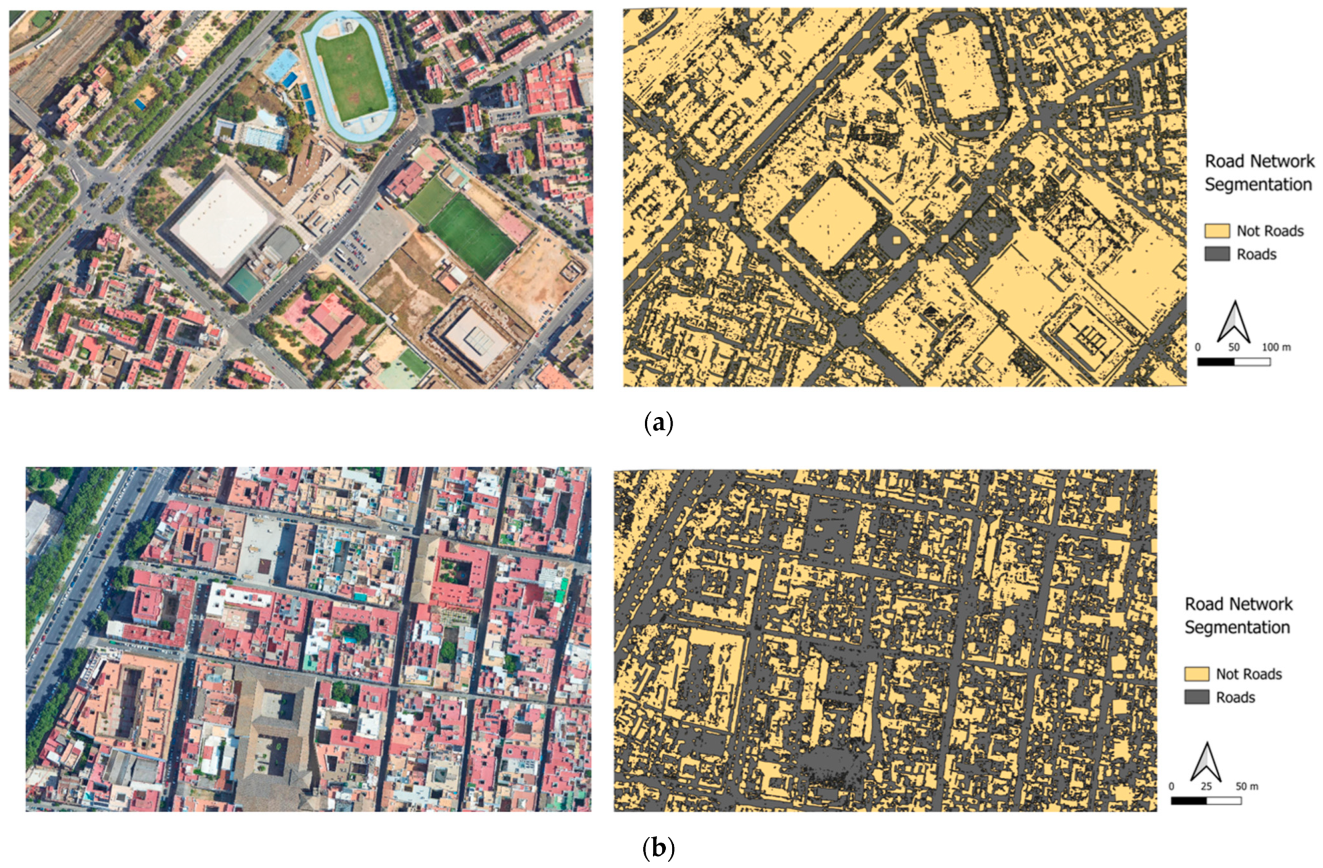
Beyond extraction, deep learning enables pattern recognition and typology classification in urban form. Trained models can analyse street Connectivity and identify morphological patterns that correlate with environmental and social risks. An example of using the Deepness plugin to identify and segment road networks is shown in Figure 16.
The segmentation of road networks is performed in QGIS using the Deepness plugin in selected areas in Zone M and Zone W. These insights may in the future complement the Space Syntax theory by identifying how spatial structure relates to heat exposure, accessibility, or segregation. A particularly promising application is the use of deep learning to predict Space Syntax indicators from spatial data inputs. Trained models can act as surrogate estimators of integration or Connectivity, allowing for faster, scalable spatial analysis without requiring full DepthmapX simulations. When integrated, deep learning and syntactic analysis offer a powerful diagnostic framework for identifying HBs.

4.4.2. Future Deep Learning Prospect of Research Advantages

Researchers can streamline data integration and visualization, making advanced heat mapping more accessible for urban planners and policymakers. Moreover, coupling deep learning with time-series remote sensing and participatory datasets allows for adaptive, equity-oriented urban planning under evolving climate conditions. This integration is especially beneficial in rapidly urbanizing or data-scarce regions, where real-time, scalable solutions are essential for addressing environmental injustice and building climate resilience. The key objective of this study is to identify Heat Boundaries; hence, the automation of this task, as shown in Table 8, will provide a more efficient and accurate means of delineating thermal hotspots across diverse urban landscapes.
By leveraging deep learning algorithms, the process of identifying HBs becomes less reliant on manual interpretation, reducing both time consumption and potential human error. Furthermore, automated detection enables the analysis of large-scale and high-resolution datasets, facilitating the monitoring of heat distribution dynamics over time. This capability is critical for informing targeted interventions, optimizing resource allocation, and promoting equitable climate adaptation strategies that prioritize vulnerable communities (Figure 17).

5. Conclusions

This study presents a multidimensional framework to assess urban heat vulnerability in Seville by integrating remote sensing, spatial configuration, and social vulnerability indicators across two contrasting climatic scenarios: a heatwave (June 26, 2023) and a normal summer day (14 July 2024). The results confirm significant intra-urban disparities in both daytime and nighttime Land Surface Temperatures, closely aligned with patterns of social disadvantage, urban morphology, and spatial segregation.
Peripheral zones and industrial clusters recorded the highest daytime LSTs—exceeding 53 °C during the heatwave—particularly in areas with barren land, high built-up density (NDBI), and minimal vegetation (low NDVI). In contrast, river-adjacent and historically dense neighbourhoods exhibited lower temperatures, benefiting from traditional urban form, shading, and proximity to water bodies. At night, thermal patterns shifted: densely built central districts retained more heat than peripheral areas, highlighting the compound vulnerability of socially disadvantaged neighbourhoods.
Average LST values across zones also followed a clear spatial pattern: in 2023, the peripheries averaged 43.65 °C, compared to 42.03 °C in Zone M and 36.74 °C in Zone W (a difference of 5.63 °C between peripheries and Zone W, and 5.29 °C between Zone M and Zone W). In 2024, these averages were slightly lower but consistent, at 39.85 °C (peripheries), 38.63 °C (Zone M), and 36.08 °C (Zone W) (a difference of 3.77 °C between peripheries and Zone W, and 2.55 °C between Zone M and Zone W). These patterns confirm that socially disadvantaged and morphologically exposed areas are consistently hotter, with differences ranging from 2.55 °C to 5.63 °C, depending on the scenario and zone comparison. These LST distributions align with NDVI and NDBI metrics. Neighbourhoods with critical or severe vulnerability scores exhibited low NDVI and high NDBI values—indicating sparse vegetation and dense built-up areas.
This study introduces the concept of Heat Boundaries (HBs) as persistent high-temperature zones that act as thermal and morphological barriers, often bordering the most vulnerable communities. HBs make up approximately 17% of Seville’s urban fabric, dominated by barren land (42%), industrial areas (30%), and transport infrastructure (28%). The highest social vulnerability index (SVI = 4) was observed in Los Pájaros (M1) and Polígono Sur (S1), which also reported some of the highest LST values in both scenarios, reinforcing the co-location of heat exposure and social marginalization.
Statistical correlations reinforce the centrality of built intensity and vegetation in shaping thermal exposure. While most Space Syntax indicators showed weak associations with LST, Mean Depth emerged as a critical Space Syntax measure, higher values corresponded with greater thermal stress, particularly during heatwaves and nighttime conditions, indicating that spatial segregation amplifies vulnerability.
Correlation analysis confirms these findings quantitatively. Average LST demonstrated strong positive correlations with average NDBI (Pearson’s r = 0.43 in 2023; r = 0.28 in 2024) and moderate inverse relationships with average NDVI, particularly during the heatwave scenario where NDVI Average and LST Average showed a Pearson’s r of −0.43. These relationships support the respective roles of built-up surfaces in heat intensification and vegetation in thermal mitigation. Conversely, the relationship between LST and Space Syntax metrics was weak, with Mean Depth showing only moderate correlations (r = 0.49 in 2023; r = 0.47 in 2024), underlining the need to integrate multiple spatial and environmental datasets for more robust heat vulnerability models. The correlation between average LST and social vulnerability (SVI) was moderate and statistically significant during the heatwave (r = 0.35, p = 0.05), though this relationship weakened under normal summer conditions (r = 0.27, p = 0.14).
This research contributes to advancing urban heat vulnerability assessments by:
  • Establishing a scalable method to delineate and classify HBs using remote sensing and LULC patterns.
  • Demonstrating the value of integrating spatial configuration metrics in urban heat risk analysis.
  • Highlighting the role of social vulnerability in compounding heat exposure.
Policy recommendations include rehabilitating Heat Boundaries through greening interventions, enhancing shade and permeability in vulnerable neighbourhoods, and reconfiguring street networks to improve Connectivity and airflow. Initial experimentation with the Deepness plugin in QGIS 3.38 suggests that machine learning holds promise for automating HB detection and high-resolution thermal mapping, though further work is needed to improve model accuracy and cross-scale data integration.
In summary, this research provides a comprehensive, equity-oriented framework for diagnosing and mitigating urban heat vulnerability. It shows that heat exposure is not only a climatological challenge but also a spatial and social one—shaped by Land Use, infrastructure, and inequality. As climate extremes intensify, the integration of geospatial analytics, urban morphology, and socio-demographic data will be essential for building adaptive and just cities. The case of Seville offers valuable insights into and a transferable model for other urban contexts facing similar heat-related challenges.

Author Contributions

Conceptualization, S.A. and A.G.-M.; methodology, S.A.; software, S.A.; validation, S.A., W.A.-A., and V.P.L.-C.; formal analysis, S.A.; investigation, S.A.; resources, S.A.; data curation, S.A.; writing—original draft preparation, S.A.; writing—review and editing, A.G.-M., V.P.L.-C., and W.A.-A.; visualization, S.A.; supervision, A.G.-M. and V.P.L.-C. All authors have read and agreed to the published version of the manuscript.

Funding

This research article received no external funding.

Data Availability Statement

Data will be provided upon request.

Conflicts of Interest

The authors declare no conflicts of interest.

Abbreviations

The following abbreviations are used in this manuscript:
AOIArea of Interest
AOIsAreas of Interest
CBsCooling Boundaries
CNNsConvolutional Neural Networks
GISsGeographic Information Systems
HB/HBsHeat Boundary/Heat Boundaries
INEInstituto Nacional de Estadística (Spanish National Institute of Statistics)
LCZsLocal Climate Zones
LSTLand Surface Temperature
LULCLand Use and Land Cover
MIVAUMinisterio de la Vivienda y Agenda Urbana (Ministry of Housing and Urban Agenda)
NDVINormalized Difference Vegetation Index
NDBINormalized Difference Built-Up Index
OLIOperational Land Imager
ONNXOpen Neural Network Exchange
SVISocial Vulnerability Index
TIRSThermal Infrared Sensor
UCIsUrban Cool Islands
UCLUniversity College London
UHIsUrban Heat Islands
USGSUnited States Geological Survey
VNsVulnerable Neighbourhoods

References

  1. Degirmenci, K.; Desouza, K.C.; Fieuw, W.; Watson, R.T.; Yigitcanlar, T. Understanding Policy and Technology Responses in Mitigating Urban Heat Islands: A Literature Review and Directions for Future Research. Sustain. Cities Soc. 2021, 70, 102873. [Google Scholar] [CrossRef]
  2. Pena Acosta, M.; Vahdatikhaki, F.; Santos, J.; Dorée, A.G. A Comparative Analysis of Surface and Canopy Layer Urban Heat Island at the Micro Level Using a Data-Driven Approach. Sustain. Cities Soc. 2023, 99, 104944. [Google Scholar] [CrossRef]
  3. Peng, W.; Wang, R.; Duan, J.; Gao, W.; Fan, Z. Surface and Canopy Urban Heat Islands: Does Urban Morphology Result in the Spatiotemporal Differences? Urban Clim. 2022, 42, 101136. [Google Scholar] [CrossRef]
  4. Voogt, J.A.; Oke, T.R. Thermal Remote Sensing of Urban Climates. Remote Sens. Environ. 2003, 86, 370–384. [Google Scholar] [CrossRef]
  5. Li, X.; Zhou, Y.; Yu, S.; Jia, G.; Li, H.; Li, W. Urban Heat Island Impacts on Building Energy Consumption: A Review of Approaches and Findings. Energy 2019, 174, 407–419. [Google Scholar] [CrossRef]
  6. Wang, S.; Cai, W.; Tao, Y.; Sun, Q.C.; Wong, P.P.Y.; Huang, X.; Liu, Y. Unpacking the Inter- and Intra-Urban Differences of the Association between Health and Exposure to Heat and Air Quality in Australia Using Global and Local Machine Learning Models. Sci. Total Environ. 2023, 871, 162005. [Google Scholar] [CrossRef] [PubMed]
  7. Ho, J.Y.; Shi, Y.; Lau, K.K.L.; Ng, E.Y.Y.; Ren, C.; Goggins, W.B. Urban Heat Island Effect-Related Mortality under Extreme Heat and Non-Extreme Heat Scenarios: A 2010–2019 Case Study in Hong Kong. Sci. Total Environ. 2023, 858, 159791. [Google Scholar] [CrossRef] [PubMed]
  8. Ellena, M.; Breil, M.; Soriani, S. The Heat-Health Nexus in the Urban Context: A Systematic Literature Review Exploring the Socio-Economic Vulnerabilities and Built Environment Characteristics. Urban Clim. 2020, 34, 100676. [Google Scholar] [CrossRef]
  9. Mitchell, B.C.; Chakraborty, J. Exploring the Relationship between Residential Segregation and Thermal Inequity in 20 U.S. Cities. Local Environ. 2018, 23, 796–813. [Google Scholar] [CrossRef]
  10. Hashemi, A.; Dungrani, M. Indoor Environmental Quality and Health Implications of Building Retrofit and Occupant Behaviour in Social Housing. Sustainability 2025, 17, 264. [Google Scholar] [CrossRef]
  11. Esposito, A.; Pappaccogli, G.; Donateo, A.; Salizzoni, P.; Maffeis, G.; Semeraro, T.; Santiago, J.L.; Buccolieri, R. Urban Morphology and Surface Urban Heat Island Relationship During Heat Waves: A Study of Milan and Lecce (Italy). Remote Sens. 2024, 16, 4496. [Google Scholar] [CrossRef]
  12. Zou, Z.; Yan, C.; Yu, L.; Jiang, X.; Ding, J.; Qin, L.; Wang, B.; Qiu, G. Impacts of Land Use/ Land Cover Types on Interactions between Urban Heat Island Effects and Heat Waves. Build. Environ. 2021, 204, 108138. [Google Scholar] [CrossRef]
  13. Makvandi, M.; Li, W.; Li, Y.; Wu, H.; Khodabakhshi, Z.; Xu, X.; Yuan, P. Advancing Urban Resilience Amid Rapid Urbanization: An Integrated Interdisciplinary Approach for Tomorrow’s Climate-Adaptive Smart Cities—A Case Study of Wuhan, China. Smart Cities 2024, 7, 2110–2130. [Google Scholar] [CrossRef]
  14. Aslanoğlu, R.; Kazak, J.K.; Szewrański, S.; Świąder, M.; Arciniegas, G.; Chrobak, G.; Jakóbiak, A.; Turhan, E. Ten Questions Concerning the Role of Urban Greenery in Shaping the Future of Urban Areas. Build. Environ. 2025, 267, 112154. [Google Scholar] [CrossRef]
  15. Guan, S.; Hu, H. Exploring the Potential Relationship between Cooling Green Space and Built-up Area: Analysis of Community Green Space Characteristics Based on GWPCA. Build. Environ. 2025, 267, 112190. [Google Scholar] [CrossRef]
  16. Soltanifard, H.; Aliabadi, K. Impact of Urban Spatial Configuration on Land Surface Temperature and Urban Heat Islands: A Case Study of Mashhad, Iran. Theor. Appl. Climatol. 2019, 137, 2889–2903. [Google Scholar] [CrossRef]
  17. Zhang, Y.; Wu, Q.; Wu, L.; Li, Y. Measuring Community Green Inequity: A Fine-Scale Assessment of Beijing Urban Area. Land 2021, 10, 1197. [Google Scholar] [CrossRef]
  18. Sharifi, A. Resilient Urban Forms: A Review of Literature on Streets and Street Networks. Build. Environ. 2019, 147, 171–187. [Google Scholar] [CrossRef]
  19. Hong, C.; Qu, Z.; Xiao, R.; Wang, Z.; Yang, Y.; Qian, J.; Zhang, C.; Zhang, Y.; Li, X.; Dong, Z.; et al. Vertical Thermal Environment Investigation in Different Urban Zones (LCZ4/LCZ6/LCZA) and Heat Mitigation Evaluation: Field Measurements and Numerical Simulations. Build. Environ. 2024, 262, 111840. [Google Scholar] [CrossRef]
  20. Nasehi, S.; Yavari, A.; Salehi, E.; Emmanuel, R. Role of Local Climate Zone and Space Syntax on Land Surface Temperature (Case Study: Tehran). Urban Clim. 2022, 45, 101245. [Google Scholar] [CrossRef]
  21. Eldesoky, A.H.; Gil, J.; Pont, M.B. Combining Environmental and Social Dimensions in the Typomorphological Study of Urban Resilience to Heat Stress. Sustain. Cities Soc. 2022, 83, 103971. [Google Scholar] [CrossRef]
  22. Shmelev, S.E.; Shmeleva, I.A. Smart and Sustainable Benchmarking of Cities and Regions in Europe: The Application of Multicriteria Assessment. Cities 2025, 156, 105533. [Google Scholar] [CrossRef]
  23. Daniel, C.; Pettit, C. The Use of Urban Analytics in Strategic Planning—A Case Study of the Greater Sydney Region Plan. Comput. Environ. Urban Syst. 2025, 117, 102249. [Google Scholar] [CrossRef]
  24. Liu, P.; Lei, B.; Huang, W.; Biljecki, F.; Wang, Y.; Li, S.; Stouffs, R. Sensing Climate Justice: A Multi-Hyper Graph Approach for Classifying Urban Heat and Flood Vulnerability through Street View Imagery. Sustain. Cities Soc. 2025, 118, 106016. [Google Scholar] [CrossRef]
  25. Mohammad Harmay, N.S.; Choi, M. The Urban Heat Island and Thermal Heat Stress Correlate with Climate Dynamics and Energy Budget Variations in Multiple Urban Environments. Sustain. Cities Soc. 2023, 91, 104422. [Google Scholar] [CrossRef]
  26. Xu, C.; Chen, G.; Huang, Q.; Su, M.; Rong, Q.; Yue, W.; Haase, D. Can Improving the Spatial Equity of Urban Green Space Mitigate the Effect of Urban Heat Islands? An Empirical Study. Sci. Total Environ. 2022, 841, 156687. [Google Scholar] [CrossRef]
  27. Herrera-Acevedo, D.D.; Sierra-Porta, D. Network Structure and Urban Mobility Sustainability: A Topological Analysis of Cities from the Urban Mobility Readiness Index. Sustain. Cities Soc. 2025, 119, 106076. [Google Scholar] [CrossRef]
  28. Li, P.; Wu, W.; Yin, Y. Enhanced Accessibility to Park Cooling Services in Developed Areas: Experimental Insights on the Walkability in Large Urban Agglomerations. Build. Environ. 2025, 272, 112665. [Google Scholar] [CrossRef]
  29. Li, F.; Yigitcanlar, T.; Li, W.; Nepal, M.; Nguyen, K.; Dur, F. Understanding Urban Heat Vulnerability: Scientometric Analysis of Five Decades of Research. Urban Clim. 2024, 56, 102035. [Google Scholar] [CrossRef]
  30. Vaňo, S.; Duchková, H.; Bašta, P.; Jančovič, M.; Geletič, J.; Lorencová, E.K.; Suchá, L. From Scenarios to Strategies: Integrated Methodology for Addressing Urban Heat Vulnerability in an Uncertain Future. Sustain. Cities Soc. 2025, 121, 106202. [Google Scholar] [CrossRef]
  31. Karanja, J.; Kiage, L. Perspectives on Spatial Representation of Urban Heat Vulnerability. Sci. Total Environ. 2021, 774, 145634. [Google Scholar] [CrossRef]
  32. Yamu, C.; van Nes, A.; Garau, C. Bill Hillier’s Legacy: Space Syntax—A Synopsis of Basic Concepts, Measures, and Empirical Application. Sustainability 2021, 13, 3394. [Google Scholar] [CrossRef]
  33. Sennett, R. The Open City. In In The Post-Urban World; Haas, T., Westlund, H., Eds.; Routledge: New York, NY, USA, 2018; pp. 97–105. [Google Scholar]
  34. Sennett, R. Reflections on the Public Realm. In A Companion to the City; Wiley: Hoboken, NJ, USA, 2003; pp. 380–387. [Google Scholar]
  35. Hillier, B. Space and Spatiality: What the Built Environment Needs from Social Theory. Build. Res. Inf. 2008, 36, 216–230. [Google Scholar] [CrossRef]
  36. Hillier, B.; Hanson, J. The Social Logic of Space; Cambridge University Press: Cambridge, UK, 1984; ISBN 9780521233651. [Google Scholar]
  37. Varamesh, S.; Mohtaram Anbaran, S.; Shirmohammadi, B.; Al-Ansari, N.; Shabani, S.; Jaafari, A. How Do Different Land Uses/Covers Contribute to Land Surface Temperature and Albedo? Sustainability 2022, 14, 16963. [Google Scholar] [CrossRef]
  38. Jiang, F.; Ma, J. Predicting Urban Vitality at Regional Scales: A Deep Learning Approach to Modelling Population Density and Pedestrian Flows. Smart Cities 2025, 8, 58. [Google Scholar] [CrossRef]
  39. Adegun, A.A.; Fonou-Dombeu, J.V.; Viriri, S.; Odindi, J. Ontology-Based Deep Learning Model for Object Detection and Image Classification in Smart City Concepts. Smart Cities 2024, 7, 2182–2207. [Google Scholar] [CrossRef]
  40. USGS. Available online: https://www.usgs.gov/ (accessed on 22 March 2025).
  41. QGIS. Available online: https://qgis.org/ (accessed on 22 March 2025).
  42. Earth Data AppEEARS. Available online: https://appeears.earthdatacloud.nasa.gov/ (accessed on 24 July 2025).
  43. INE. Available online: https://www.ine.es/ (accessed on 22 March 2025).
  44. MIVAU. Available online: https://www.mivau.gob.es/ (accessed on 22 March 2025).
  45. Municipality of Seville. Available online: https://www.sevilla.org/ (accessed on 22 March 2025).
  46. Spanish Meteorological Agency AEMET. Available online: https://www.aemet.es/es/eltiempo/observacion/ultimosdatos?k=and&l=5783 (accessed on 22 March 2025).
  47. Halder, B.; Karimi, A.; Mohammad, P.; Bandyopadhyay, J.; Brown, R.D.; Yaseen, Z.M. Investigating the Relationship between Land Alteration and the Urban Heat Island of Seville City Using Multi-Temporal Landsat Data. Theor. Appl. Climatol. 2022, 150, 613–635. [Google Scholar] [CrossRef]
  48. Marchena Gómez, M.J.; Hernández Martín, E. Sevilla En La Primera Década Del Siglo XXI: Transformaciones Urbanas Hacia Un Nuevo Modelo de Ciudad. Boletín Asoc. Geógrafos Españoles 2016. [Google Scholar] [CrossRef]
  49. Diaz-Parra, I.; Jover, J. Overtourism, Place Alienation and the Right to the City: Insights from the Historic Centre of Seville, Spain. J. Sustain. Tour. 2021, 29, 158–175. [Google Scholar] [CrossRef]
  50. Jadraque Gago, E.; Etxebarria Berrizbeitia, S.; Pacheco Torres, R.; Muneer, T. Effect of Land Use/Cover Changes on Urban Cool Island Phenomenon in Seville, Spain. Energies 2020, 13, 3040. [Google Scholar] [CrossRef]
  51. Fernández, I.C.; Wu, J. A GIS-Based Framework to Identify Priority Areas for Urban Environmental Inequity Mitigation and Its Application in Santiago de Chile. Appl. Geogr. 2018, 94, 213–222. [Google Scholar] [CrossRef]
  52. Buckland, M.; Pojani, D. Green Space Accessibility in Europe: A Comparative Study of Five Major Cities. Eur. Plan. Stud. 2023, 31, 146–167. [Google Scholar] [CrossRef]
  53. García-Pardo, K.A.; Moreno-Rangel, D.; Domínguez-Amarillo, S.; García-Chávez, J.R. Remote Sensing for the Assessment of Ecosystem Services Provided by Urban Vegetation: A Review of the Methods Applied. Urban For. Urban Green. 2022, 74, 127636. [Google Scholar] [CrossRef]
  54. García, D.H. Analysis of Urban Heat Island and Heat Waves Using Sentinel-3 Images: A Study of Andalusian Cities in Spain. Earth Syst. Environ. 2022, 6, 199–219. [Google Scholar] [CrossRef]
  55. Sun, M.; Meng, Q. Using Spatial Syntax and GIS to Identify Spatial Heterogeneity in the Main Urban Area of Harbin, China. Front. Earth Sci. 2022, 10, 893414. [Google Scholar] [CrossRef]
  56. Ong, B.L. Green Plot Ratio: An Ecological Measure for Architecture and Urban Planning. Landsc. Urban Plan. 2003, 63, 197–211. [Google Scholar] [CrossRef]
  57. Chen, S.; Haase, D.; Qureshi, S.; Firozjaei, M.K. Integrated Land Use and Urban Function Impacts on Land Surface Temperature: Implications on Urban Heat Mitigation in Berlin with Eight-Type Spaces. Sustain. Cities Soc. 2022, 83, 103944. [Google Scholar] [CrossRef]
  58. Euro News. Available online: https://www.euronews.com/green/2023/06/26/heatwave-yago-dangerous-heat-event-named-in-seville-for-the-second-time-ever (accessed on 26 July 2025).
  59. AEMET Heatwave Data. Available online: https://www.aemet.es/documentos/es/serviciosclimaticos/vigilancia_clima/resumenes_climat/mensuales/2023/res_mens_clim_2023_06.pdf (accessed on 26 July 2025).
  60. AEMET Non-Heatwave Data. Available online: https://www.aemet.es/documentos/es/serviciosclimaticos/vigilancia_clima/resumenes_climat/ccaa/andalucia-ceuta-melilla/avance_climat_acm_jul_2024.pdf (accessed on 26 July 2025).
  61. Tucker, C.J. Red and Photographic Infrared Linear Combinations for Monitoring Vegetation. Remote Sens. Environ. 1979, 8, 127–150. [Google Scholar] [CrossRef]
  62. Zha, Y.; Gao, J.; Ni, S. Use of Normalized Difference Built-up Index in Automatically Mapping Urban Areas from TM Imagery. Int. J. Remote Sens. 2003, 24, 583–594. [Google Scholar] [CrossRef]
  63. Plan Local de Intervención En Zonas Desfavorecidas. Available online: https://www.sevilla.org/servicios/servicios-sociales/publicaciones/plan-local-de-intervencion-en-zonas-desfavorecidas (accessed on 22 March 2025).
  64. Hu, Y.; Gao, S.; Janowicz, K.; Yu, B.; Li, W.; Prasad, S. Extracting and Understanding Urban Areas of Interest Using Geotagged Photos. Comput. Environ. Urban Syst. 2015, 54, 240–254. [Google Scholar] [CrossRef]
  65. Patel, S.; Indraganti, M.; Jawarneh, R.N. A Comprehensive Systematic Review: Impact of Land Use/ Land Cover (LULC) on Land Surface Temperatures (LST) and Outdoor Thermal Comfort. Build. Environ. 2024, 249, 111130. [Google Scholar] [CrossRef]
  66. Wang, Z.; Zhou, R.; Yu, Y. The Impact of Urban Morphology on Land Surface Temperature under Seasonal and Diurnal Variations: Marginal and Interaction Effects. Build. Environ. 2025, 272, 112673. [Google Scholar] [CrossRef]
  67. Wang, H.; Yi, T.; Lu, Y.; Wang, Y.; Wu, J. Patterns of Nighttime Surface Urban Heat Island Patch in Mega Urban Agglomerations: A Case Study in the Pearl River Delta, China. Sustain. Cities Soc. 2025, 128, 106465. [Google Scholar] [CrossRef]
  68. Zhao, J.; Yu, L.; Zhao, L.; Fu, H.; Gong, P. Asymmetric Influence of Urban Morphology Changes on Land Surface Temperature between Daytime and Nighttime. Sustain. Cities Soc. 2025, 124, 106307. [Google Scholar] [CrossRef]
  69. van den Heuvel, E.; Zhan, Z. Myths About Linear and Monotonic Associations: Pearson’s r, Spearman’s ρ, and Kendall’s τ. Am. Stat. 2022, 76, 44–52. [Google Scholar] [CrossRef]
  70. Zhang, L.; Bagan, H.; Chen, C.; Yoshida, T. Exploring the Impact of Urban Morphology on River Cooling Effects: A Case Study of the Arakawa River in Tokyo. Ecol. Indic. 2025, 172, 113288. [Google Scholar] [CrossRef]
  71. Kim, Y.; Yoo, C.; Im, J. Nighttime Satellite Land Surface Temperature for Urban Applications: Achievements, Challenges, and Future Prospects. GISci. Remote Sens. 2025, 62, 2527990. [Google Scholar] [CrossRef]
  72. Kustura, K.; Conti, D.; Sammer, M.; Riffler, M. Harnessing Multi-Source Data and Deep Learning for High-Resolution Land Surface Temperature Gap-Filling Supporting Climate Change Adaptation Activities. Remote Sens. 2025, 17, 318. [Google Scholar] [CrossRef]
  73. Adegun, A.A.; Viriri, S.; Tapamo, J.-R. Review of Deep Learning Methods for Remote Sensing Satellite Images Classification: Experimental Survey and Comparative Analysis. J. Big Data 2023, 10, 93. [Google Scholar] [CrossRef]
  74. Li, F.; Yigitcanlar, T.; Nepal, M.; Thanh, K.N.; Dur, F. A Novel Urban Heat Vulnerability Analysis: Integrating Machine Learning and Remote Sensing for Enhanced Insights. Remote Sens. 2024, 16, 3032. [Google Scholar] [CrossRef]
  75. Cheng, X.; Sun, Y.; Zhang, W.; Wang, Y.; Cao, X.; Wang, Y. Application of Deep Learning in Multitemporal Remote Sensing Image Classification. Remote Sens. 2023, 15, 3859. [Google Scholar] [CrossRef]
  76. Aszkowski, P.; Ptak, B.; Kraft, M.; Pieczyński, D.; Drapikowski, P. Deepness: Deep Neural Remote Sensing Plugin for QGIS. SoftwareX 2023, 23, 101495. [Google Scholar] [CrossRef]
  77. Vali, A.; Comai, S.; Matteucci, M. Deep Learning for Land Use and Land Cover Classification Based on Hyperspectral and Multispectral Earth Observation Data: A Review. Remote Sens. 2020, 12, 2495. [Google Scholar] [CrossRef]
  78. Gharahbagh, A.A.; Hajihashemi, V.; Machado, J.J.M.; Tavares, J.M.R.S. Land Cover Classification Model Using Multispectral Satellite Images Based on a Deep Learning Synergistic Semantic Segmentation Network. Sensors 2025, 25, 1988. [Google Scholar] [CrossRef]
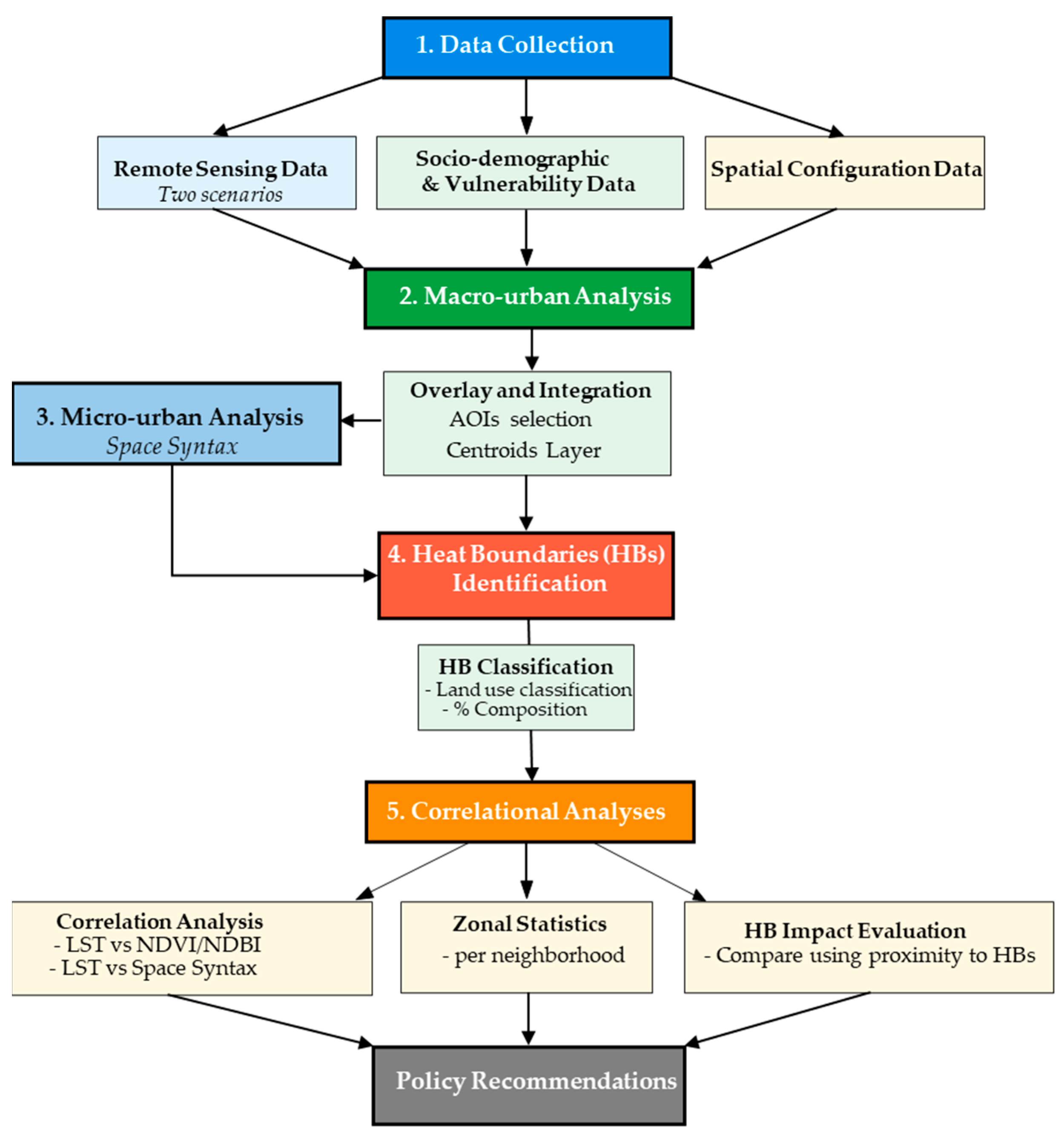
Figure 1. Methodology workflow.
Smartcities 08 00137 g001
Figure 2. Data Centroids layer in QGIS.
Smartcities 08 00137 g002
Figure 3. (a) Location of Seville in Andalusia in Spain; (b) Map of Seville with districts.
Smartcities 08 00137 g003
Figure 4. Remote sensing data for Seville during two scenarios: heatwave scenario on 26 June 2023 and non-heatwave scenario on 14 July 2024, 11:00 AM GMT, daytime LST 2023 (a); Daytime LST 2024 (b) NDVI 2023 (c); NDVI 2024 (d); NDBI 2023 (e); NDBI 2024 (f).
Smartcities 08 00137 g004
Figure 5. (a) Population density by district in Seville for 2023 (people/sq.km) [45]; (b) Vulnerable neighbourhoods in Seville in 2011 [44]; (c) Neighbourhoods with disadvantaged areas (2018–2022) [63].
Smartcities 08 00137 g005
Figure 6. Combined map of macro-urban layers, including LST, population density, vulnerability maps, and delineation of abstract locations of micro-urban Areas of Interest (AOIs).
Smartcities 08 00137 g006
Figure 7. Micro-urban Areas of Interest (AOIs): M and W; about 7.5 sq.km each.
Smartcities 08 00137 g007
Figure 8. Periphery neighbourhoods in Seville (P1–P7).
Smartcities 08 00137 g008
Figure 9. Vulnerable neighbourhoods in Zone S, and the industrial zone “El Juncal-Híspalis” in the South.
Smartcities 08 00137 g009
Figure 10. Nighttime LST (°C) generated from ECOSTRESS data corresponding to (a) the heatwave night of June 26, 2023, and (b) the non-heatwave night of July 14, 2024.
Smartcities 08 00137 g010
Figure 11. (a) Google map of Zone M. (b) Urban grain displaying LULC zoning. (c) Centroids map illustrating LST distribution. (d) Space Syntax analysis for Zone M, showing values for Connectivity, Integration, and Mean Depth.
Smartcities 08 00137 g011
Figure 12. (a) Google map of Zone W. (b) Urban grain displaying LULC zoning. (c) Centroids map illustrating LST distribution. (d) Space Syntax analysis for Zone W, showing values for Connectivity, Integration, and Mean Depth.
Smartcities 08 00137 g012
Figure 13. Mapping of Heat Boundaries (HBs) in Seville during the daytime, including transportation hubs, industrial zones, and barren lands, along with cooling boundaries, such as the parks and the river, in both the heatwave scenario in 2023 (a) and the non-heatwave scenario in 2024 (b).
Smartcities 08 00137 g013aSmartcities 08 00137 g013b
Figure 14. Mapping of Heat Boundaries (HBs) in Seville during the nighttime showing transportation hubs, industrial zones, and barren lands, along with cooling boundaries, such as the parks and the river, in both the heatwave scenario in 2023 (a) and the non-heatwave scenario in 2024 (b).
Smartcities 08 00137 g014
Figure 15. Segmentation of Cooling Boundaries (CBs) (the river and green areas) in a selected sample area in Zone W, performed using the Deepness plugin in QGIS, using a pre-trained ONNX model.
Smartcities 08 00137 g015
Figure 16. Segmentations of road networks in a selected sample area in Zone M (a) and sample area in Zone W (b), performed using the Deepness plugin in QGIS, using a pre-trained ONNX model.
Smartcities 08 00137 g016
Figure 17. Key stages of both methods for the identification of Heat Boundaries.
Smartcities 08 00137 g017
Table 1. Datasets and variables.
Datasets and VariablesDescriptionDateSourceTool Scale Applied in Study
Remote Sensing Data
LSTRaster layers indicating daytime urban heat data generated using bands 10 and 11
Raster layers indicating nighttime urban heat data
26 June 2023,
14 July 2024
Landsat 9 [40]
ECOSTRESS [42]
QGISMacro-urban
NDVIRaster layers data indicating vegetation generated using bands 4 and 526 June 2023,
14 July 2024
Landsat 9 [40]QGISMacro-urban
NDBIRaster layers data indicating built area generated using bands 5 and 626 June 2023,
14 July 2024
Landsat 9 [40]QGISMacro-urban
Socio-Demographical Data
Population densityPopulation density people/sq.km2023Municipality of Seville [45] Macro-urban
VulnerabilityVulnerable neighbourhoods based on socioeconomic data
Disadvantaged areas
2011
2018
Ministry of Housing and Urban Agenda [44]
Municipality of Seville [45]
Macro-urban
Spatial Configuration Data
ConnectivityMeasures the number of spaces immediately connecting a space of origin2025Space Syntax theory [36]DepthmapXMicro-urban
IntegrationRefers to the degree of spatial aggregation or dispersion between a space and other spaces in the system. The higher the value, the higher the accessibility and commonality of the space2025Space Syntax theory [36]DepthmapXMicro-urban
Mean DepthRefers to the shortest topological distance of the space from all other spaces; the lower the value, the more convenient the space is.2025Space Syntax theory [36]DepthmapXMicro-urban
Table 2. Remote sensing diurnal data for neighbourhoods in AOIs in Seville for 26 June 2023 during a heatwave scenario.
RefNeighbourhoodLST (°C)NDVINDBISocial Vulnerability Index SVI
MeanMax MinMeanMax MinMeanMax Min
Zone M
M1Los Pájaros42.4643.6640.430.120.310.050.000.120.194
M2San Pablo A + B 41.9743.2740.950.140.240.05−0.020.08−0.122
M3San Pablo C43.6446.2440.100.140.510.03−0.030.19−0.312
M4San Pablo D + E41.6144.1340.390.140.290.06−0.030.12−0.182
M5Amate42.7543.8041.120.130.320.040.000.11−0.163
M6Santa Aurelia41.7947.1637.590.190.460.02−0.050.11−0.252
Zone N
N1Polígono Norte41.5743.3740.580.150.280.05−0.030.07−0.162
N2San Jeronimo42.4444.0540.850.130.350.040.000.11−0.212
N3El Rocio42.0842.6641.610.130.240.06−0.010.05−0.091
N4Begona Santa Catalina 42.1543.3741.100.120.370.060.020.13−0.232
N5PIO XII42.2843.1641.520.110.170.060.020.110.172
Zone S
S1Polígono Sur42.9751.2136.690.170.41−0.01−0.010.14−0.273
S2Las letanias- Paz y Amistad42.9253.9930.150.160.61−0.20−0.010.37−0.434
S3El Cerro43.0548.4141.090.120.360.030.020.11−0.202
S4Tiro de Linea-Santa Genoveva42.0043.8340.680.110.270.010.010.08−0.131
Zone E
E1Rochelambert42.4243.3641.450.120.300.020.000.15−0.162
E2Palmete44.6048.7640.380.110.270.010.010.08−0.132
E3Parque Alcosa—Jardines del Eden42.7245.7440.570.150.430.03−0.010.14−0.262
E4La Plata42.8643.9741.110.110.320.010.020.17−0.183
E5Juan XXIII42.2145.2040.940.130.310.02−0.010.14−0.161
Zone W
W1San Lorenzo39.3142.6931.160.100.39−0.07−0.010.10−0.260
W2San Vicente35.9538.9229.660.100.44−0.15−0.01−0.280.110
W3Museo36.5240.2230.490.090.43−0.12−0.02−0.230.120
W4Arenal36.4140.2631.080.080.39−0.130.01−0.230.180
W5Santa Cruz35.5038.4430.750.150.46−0.14−0.05−0.320.120
Peripheries
P1Tablada43.6753.9930.850.120.51−0.200.020.29−0.300
P2Bellavista43.9248.6630.960.150.60−0.130.030.15−0.320
P3Torreblanca44.7548.8639.340.170.440.000.050.22−0.242
P4Colores-Entreparques44.2353.1036.380.160.50−0.090.030.31−0.300
P5Valdezorras44.6848.7238.760.190.580.010.010.12−0.340
P6El Gordillo43.1948.2534.330.230.530.03−0.040.12−0.390
P7La Bachillera43.6847.4039.780.110.42−0.080.000.26−0.210
Table 3. Remote sensing diurnal data for neighbourhoods in AOIs in Seville for 14 July 2024 during a non-heatwave scenario.
RefNeighbourhoodLST (°C)NDVINDBISocial Vulnerability Index SVI
MeanMax MinMeanMax MinMeanMax Min
Zone M
M1Los Pájaros38.5739.7536.240.120.340.030.000.12−0.204
M2San Pablo A + B 37.9639.7336.770.140.270.04−0.020.21−0.132
M3San Pablo C39.9243.2235.730.150.550.02−0.040.12−0.312
M4San Pablo D + E37.9140.4236.810.140.300.05−0.030.14−0.162
M5Amate38.8039.9136.640.130.380.030.000.09−0.213
M6Santa Aurelia38.4244.6034.860.190.460.01−0.050.13−0.282
Zone N
N1Polígono Norte37.8940.2836.850.150.330.01−0.030.13−0.162
N2San Jeronimo37.5541.0930.780.140.45−0.07−0.020.11−0.242
N3El Rocio38.1238.8437.630.120.270.06−0.020.05−0.091
N4Begona Santa Catalina 38.4939.4937.860.130.430.050.000.11−0.252
N5PIO XII38.5839.8737.620.110.380.030.020.11−0.122
Zone S
S1Polígono Sur39.4249.4133.670.170.46−0.01−0.010.18−0.313
S2Las letanias- Paz y Amistad38.2440.6137.270.130.220.06−0.020.07−0.144
S3El Cerro38.9844.0536.810.120.400.010.020.14−0.312
S4Tiro de Linea-Santa Genoveva37.6939.5435.920.120.320.000.050.21−0.221
Zone E
E1Rochelambert38.4439.8336.980.120.340.040.000.17−0.182
E2Palmete40.9445.3737.320.100.45−0.030.010.21−0.252
E3ParqueAlcosa—Jardines del Eden39.1141.6136.880.150.390.01−0.010.15−0.232
E4La Plata39.1040.6637.580.100.370.000.020.22−0.213
E5Juan XXIII38.3742.5536.700.120.320.000.000.15−0.171
Zone W
W1San Lorenzo36.0038.5729.540.100.43−0.12−0.01−0.250.120
W2San Vicente35.9538.9229.660.100.44−0.15−0.01−0.280.110
W3Museo36.5240.2230.490.090.43−0.12−0.02−0.230.120
W4Arenal36.4140.2631.080.080.39−0.130.01−0.230.180
W5Santa Cruz35.5038.4430.750.150.46−0.14−0.05−0.320.120
Peripheries
P1Tablada38.2950.8127.890.130.53−0.27−0.010.27−0.350
P2Bellavista39.6148.1427.730.160.60−0.230.010.17−0.300
P3Torreblanca41.8550.1036.720.150.40−0.020.050.21−0.222
P4Colores-Entreparques40.7949.6232.460.160.50−0.120.020.33−0.350
P5Valdezorras40.2545.6632.060.200.65−0.03−0.020.19−0.470
P6El Gordillo39.3045.2730.530.250.62−0.05−0.080.12−0.440
P7La Bachillera38.8347.2229.010.210.63−0.28−0.060.24−0.470
Table 4. LST nighttime (nocturnal) LST (°C) for neighbourhoods in Seville for both scenarios: heatwave scenario of 2023 and non-heatwave scenario of 2024.
RefNeighbourhoodLST (°C)
2023 Heatwave
Night
LST (°C)
2024 Non-heatwave
Night
Social Vulnerability Index SVI
MeanMax MinMeanMax Min
Zone M
M1Los Pájaros26.9727.7725.0525.1526.3123.834
M2San Pablo A + B 27.2627.9726.0725.4225.9723.792
M3San Pablo C26.727.5925.7525.1625.9724.252
M4San Pablo D + E26.9327.6925.6925.1225.9323.372
M5Amate26.927.7526.3325.1527.5524.553
M6Santa Aurelia26.1727.6724.1124.4725.8922.572
Zone N
N1Polígono Norte27.0427.6925.8125.9126.2124.732
N2San Jeronimo25.3926.8523.1924.8826.1322.852
N3El Rocio27.5527.8727.0926.1826.6525.631
N4Begona Santa Catalina 27.4928.3327.1325.6527.0524.832
N5PIO XII27.5328.3326.8525.8326.2325.032
Zone S
S1Polígono Sur25.2628.1721.5723.8526.2121.013
S2Las letanias- Paz y Amistad27.127.9726.1525.126.3524.514
S3El Cerro26.5927.5525.3324.6526.8323.272
S4Tiro de Linea-Santa Genoveva27.2428.1926.3525.2225.5724.411
Zone E
E1Rochelambert23.9123.9123.9123.9123.9123.912
E2Palmete24.9927.0921.5123.7426.2721.152
E3ParqueAlcosa—Jardines del Eden25.8127.3723.9324.7326.2722.552
E4La Plata26.2727.0525.4524.4126.4123.393
E5Juan XXIII26.1627.2324.5324.626.5323.771
Zone W
W1San Lorenzo26.5228.0725.8525.3826.0523.750
W2San Vicente26.5427.5925.0725.1325.8923.530
W3Museo26.7828.0325.5925.3626.2923.750
W4Arenal26.9427.8526.2325.1727.4923.950
W5Santa Cruz26.7827.8925.5324.825.8323.570
Peripheries
P1Tablada24.1128.7120.7122.8325.6119.210
P2Bellavista24.5127.0921.2923.527.0520.470
P3Torreblanca23.4727.2720.5123.3625.4520.312
P4Colores-Entreparques25.0228.6121.5124.2526.9321.490
P5Valdezorras22.4326.5720.0523.0225.3321.350
P6El Gordillo22.3827.6919.2522.7326.7520.270
P7La Bachillera22.7627.4518.4122.9326.4920.030
Table 5. Axial analysis and LST data for street networks in Zones M and W during the heatwave scenario in 2023 and non-heatwave scenario in 2024 for both daytime and nighttime LSTs.
StreetLST Average (°C)LST Max (°C)ConnectivityGlobal
Integration
Mean DepthSVIAdjacent
Neighbourhoods
2023202420232024
DayNightDayNightDayNightDayNight
Zone M
C. Clemente Hidalgo41.6526.8437.8425.0742.4727.7539.2425.399623.385.174M1
41.6526.8437.8425.0742.4727.7539.2425.399053.285.482M5
Av. de Andalucía43.5325.7740.0424.5245.3027.1342.2625.3910642.776.234M1
43.5325.7740.0424.5245.3027.1342.2625.3910812.76.342M6
43.5325.7740.0424.5245.3027.1342.2625.3910432.726.292M2
Av. de Kansas City42.1026.1238.3024.4743.4427.8140.3226.1712323.365.272M2, M3, M4
Zone W
C. Torneo38.1626.6135.7625.6441.2427.5139.826.998503.195.400W1, W2, W3
Puente del Cristo de la Expiración39.5726.6335.9425.7442.4027.5138.7126.9911953.025.600W3
C. Alfonso XII41.4126.7237.2125.2141.8026.9937.6426.095602.805.950W2, W3
C. Reyes Católicos +Puente Isabel II40.0926.8835.9325.4042.1927.3738.0626.1310702.686.200W3, W4
Table 6. Correlation results for diurnal average LST (°C) as a dependent variable and the other variables in Zones (M, N, E, W, P) during the heatwave scenario in 2023 and non-heatwave scenario in 2024.
ParameterNDVI
Average
NDBI
Average
Vulnerability
SVI
2023 Heatwave Scenario
Pearson’s (r)0.430.430.35
p-value (two-tailed)0.020.010.05
Significant?YesYesYes
(alpha = 0.05)0.350.570.11
Spearman’s rank (ρ)0.350.570.11
p-value0.050.000.54
Significant? YesYesNo
2024 Non-Heatwave Scenario
Pearson’s (r)0.380.280.27
p-value (two-tailed)0.030.130.14
Significant?YesNoNo
(alpha = 0.05)0.430.280.23
Spearman’s rank (ρ)0.430.280.23
p-value0.010.120.21
Significant? YesNoNo
Table 7. Correlation results for diurnal average LST (°C) as a dependent variable and Space Syntax variables and social vulnerability index (SVI) values for the streets in Zones M and W during the heatwave scenario in 2023 and non-heatwave scenario in 2024.
Parameter ConnectivityGlobal
Integration
Mean
Depth
Vulnerability (SVI)
Year202320242023 20242023202420232024
Pearson’s (r)0.180.20−0.32−0.290.490.470.700.72
p-value (two-tailed)0.620.570.360.410.150.170.030.02
Significant?
(alpha = 0.05)
NoNoNoNoNoNoYesYes
Spearman’s rank (ρ)0.270.30−0.22−0.150.490.470.770.77
p-value0.450.410.550.670.150.170.010.01
Significant?
(alpha = 0.05)
NoNoNoNoNoNoYesYes
Sample size (n)1010101010101010
Table 8. Benefits of integrating deep learning vs. original method used in the study.
FeatureWithout Deep Learning
(Current Study)
With Deep Learning
(Proposed Extension)
Data IntegrationUses Landsat 9, ECOSTRESS, QGIS, and manual data alignment via CentroidsAutomates integration using CNNs within QGIS
Land Cover ClassificationManual extraction using NDVI/NDBI indices and Google MapsAutomated pixel-wise classification using ONNX models
LST Estimation and PredictionStatic LST maps from limited satellite dataDynamic prediction of LST using time-series models
Spatial ResolutionLimited to Landsat and ECOSTRESS resolutionsPotential to enhance resolution via super-resolution networks
Heat Boundary DetectionManual identification based on thresholdsAutomatic detection using segmentation models
Correlation AnalysisPearson’s/Spearman’s correlations between variablesNon-linear pattern recognition with attention mechanisms
Predictive CapabilitiesDescriptive analysis onlyPredictive modelling of future heat scenarios
Temporal AnalysisLimitedTime-series analysis enabled via recurrent or transformer-based models
ScalabilityLimited to SevilleScalable to other cities with minimal retraining
Space Syntax DepthmapX data integrated into QGISUsing pre-trained models to identify urban patterns and detect Space Syntax parameters
Disclaimer/Publisher’s Note: The statements, opinions and data contained in all publications are solely those of the individual author(s) and contributor(s) and not of MDPI and/or the editor(s). MDPI and/or the editor(s) disclaim responsibility for any injury to people or property resulting from any ideas, methods, instructions or products referred to in the content.